1. The beauty of $\mathbf{k_2}$

In close eccentric binaries tidal interactions lead to dynamical deformations of the stellar surfaces as the stars orbit each other. The ensuing non-spherical stellar gravitational fields in turn induce secular changes of the orbital parameters. The most prominent manifestation of this effect is the slow precession of the orbit major axis, known as apsidal motion. The rate of this motion $\dot\omega$ is directly related to the internal structure constants of each star, $k_2$, a measure of the mass distribution between the star’s core and external layers (Shakura Reference Shakura1985), mainly affected by the convective core size and internal mixing efficiency. Measuring $\dot\omega$ hence provides a powerful and independent diagnosis of the otherwise difficult to constrain density stratification inside stars and offers a unique means to reveal stars’ structure and evolution (Claret & Giménez Reference Claret and Giménez2010). This challenging technique has been known for decades, but was data and models starved until recently. Now that accurate spectroscopic and photometric data can be obtained, and that the evolution of binaries can be modelled with detailed binary stellar evolution codes, the full potential of apsidal motion can finally be exploited.

The rate of apsidal motion $\dot\omega$ is made of a Newtonian contribution $\dot\omega_{\mathrm{N}}$ – usually the dominant one – that accounts for tidal deformations and stellar rotation, and a general relativistic correction $\dot\omega_{\mathrm{GR}}$:

(1) \begin{equation}\begin{aligned}\dot\omega_\mathrm{N} = &\frac{2\pi}{P_{\mathrm{orb}}} \Bigg[15f(e)\left\{k_{2,1}q \left(\frac{R_1}{a}\right)^5 + \frac{k_{2,2}}{q} \left(\frac{R_2}{a}\right)^5\right\} \\& + g(e) \Bigg\{ k_{2,1} (1+q) \left(\frac{R_1}{a}\right)^5 \left(\frac{P_\mathrm{orb}}{P_{\mathrm{rot,1}}}\right)^2+ k_{2,2}\, \frac{1+q}{q} \left(\frac{R_2}{a}\right)^5 \left(\frac{P_\mathrm{orb}}{P_{\mathrm{rot,2}}}\right)^2 \Bigg\} \Bigg],\end{aligned}\end{equation}

\begin{equation}\dot\omega_\mathrm{GR} = \left(\frac{2\pi}{P_\mathrm{orb}}\right)^{5/3}\frac{3(G(m_1+m_2))^{2/3}}{c^2 (1-e^2)},\end{equation}

where $q=M_2/M_1$ is the mass ratio, $P_{\mathrm{orb}}$ the orbital period, a the semi-major axis of the orbit, $R_\star$ the radius, $k_{2,\star}$ the internal structure constant, and $P_{\mathrm{rot,}\star}$ the rotational period of the considered star, f(e) and g(e) functions of the eccentricity of the orbit which expressions are given in e.g., Rosu (Reference Rosu2021), G the gravitational constant, and c the speed of light. $k_2$ is an algebraic function of $\eta_2$, solution of the Clairaut-Radau differential equation that depends on the stellar density profile (Hejlesen Reference Hejlesen1987). $k_2$ is a monotonic decreasing function with time (Rosu Reference Rosu2021, their Figs 8&9); its value is mostly impacted by the density contrast at the border between the convective core and radiative envelope of the star (Rosu et al. Reference Rosu, Noels and Dupret2020a, their Fig. 1).

2. The $\mathbf{k_2}$ discrepancy

The $k_2$ discrepancy is the systematic difference between the $k_2$ values obtained from stellar evolution models and observations for massive stars: the former is systematically larger than the latter (Rosu et al. Reference Rosu, Noels and Dupret2020a; Rosu et al. Reference Rosu, Rauw and Farnir2022a; Rosu et al. Reference Rosu, Rauw and Nazé2022b). It means that models predict stars with too low a density contrast, that is to say, observations suggest that the core is more contracted and the envelope more extended. In this paper, we investigate this $k_2$ discrepancy in the benchmark twin binary HD 152248. Its twin nature – meaning that the two stars share exactly the same stellar properties – allows us to directly get $k_2$ from the observations, assuming $k_2 \equiv k_{2,1} = k_{2,2}$ in Eq. (1). The observational properties of HD 152248 are given in Table 1 (Rosu et al. Reference Rosu, Rauw and Conroy2020b). Among these properties, the radius is particularly important: it appears to the fifth power in Eq. (1), so it is important that the models do reproduce it within its error bars. The metallicity of the NGC 6231 cluster to which HD 152248 belongs is slightly super-solar: $Z=0.018\pm0.003$ (Dias et al. Reference Dias, Monteiro and Moitinho2021). The initial He abundance of the cluster is poorly-constrained as different studies achieve conflicting results: Lennon & Dufton (Reference Lennon and Dufton1983) derived a slightly super-solar while Mathys et al. (Reference Mathys, Andrievsky and Barbuy2002) a slightly sub-solar abundance.

Table 1.

Stellar and orbital parameters of HD 152248 (Rosu et al. Reference Rosu, Rauw and Conroy2020b).

Table 1 Long description

A table with 11 rows and 3 columns. The columns are labeled Parameter, Symbol, and Value. The table lists various stellar and orbital parameters of HD 152248. Row 1: Parameter, Mass; Symbol, M star (M sun); Value, 29.5 plus or minus 0.5. Row 2: Parameter, Radius; Symbol, R star (R sun); Value, 15.07 plus or minus 0.12. Row 3: Parameter, Effective temperature; Symbol, T eff star (K); Value, 34000 plus or minus 1000. Row 4: Parameter, Bolometric luminosity; Symbol, L bol star (L sun); Value, 2.73 times 10 to the power of 5. Row 5: Parameter, Internal stellar structure constant; Symbol, k 2 star; Value, 0.0010 plus or minus 0.0001. Row 6: Parameter, Surface velocity; Symbol, v surf star (km s minus 1); Value, 148 plus or minus 13. Row 7: Parameter, Mass-loss rate; Symbol, M dot (M sun yr minus 1); Value, is less than or equal to 8 times 10 to the power of minus 7. Row 8: Parameter, Nitrogen surface abundance; Symbol, N/H (nb); Value, 0.6 minus 2.2 times 10 to the power of minus 4. Row 9: Parameter, Orbital period; Symbol, P orb (d); Value, 5.816500 plus or minus 0.00002. Row 10: Parameter, Orbital eccentricity; Symbol, e; Value, 0.130 plus or minus 0.002. Row 11: Parameter, Apsidal motion rate; Symbol, omega (degree yr minus 1); Value, 1.843 plus or minus 0.083.

3. GENEC stellar evolution models

We built stellar models with the Geneva code (GENEC, Eggenberger et al. Reference Eggenberger, Meynet and Maeder2008), adopting two rotational mixing implementations, the hydrodynamic and magnetic schemes. We compare single and binary star models computed with the same internal physics. For the binary models, dynamical tides and equilibrium tides acting on small subsurface convective zones are included as described in Song et al. (Reference Song, Maeder and Meynet2013); Sciarini et al. (Reference Sciarini, Ekström and Eggenberger2024); Sciarini et al. (Reference Sciarini, Rosu and Ekström2025). We adopted the mass-loss rate of Krtička et al. (Reference Krtička, Kubát and Krtičková2024) as it best reproduces observed stars (Brands et al. Reference Brands, de Koter and Bestenlehner2022). We adopted the metallicity of the cluster and a solar initial He abundance. For the different models, we fine-tuned the initial mass $M_{\mathrm{init}}$ such that $M(R_\star) = M_\star$Footnote ¹. For the single-star models, we adopted the same approach for the surface velocity: we fine-tuned the initial velocity $v_{\mathrm{ini}}$ such that $v_{\mathrm{surf}} (R_\star) = v_{\mathrm{surf},\star}$. For binary models, we initialised the system synchronised to the orbital motion. We tested values of the overshooting parameter $\alpha_{\mathrm{ov}}$ from 0.5 to 1.0. These high values are motivated by several independent studies showing the need for larger convective boundary mixing in massive stars than anticipated and predicted from lower-mass stars in order to: reproduce the main-sequence width in the Hertzsprung-Russell (HR) diagram of stellar clusters at high masses (Castro et al. Reference Castro, Fossati and Langer2014; Baraffe et al. Reference Baraffe, Clarke and Morison2023), explain the properties of massive eclipsing binaries with 1D stellar models (Tkachenko et al. Reference Tkachenko, Pavlovski and Johnston2020; Higgins & Vink Reference Higgins and Vink2019), 2D and 3D hydrodynamic simulations (Baraffe et al. Reference Baraffe, Clarke and Morison2023; Mao et al. Reference Mao, Woodward and Herwig2024), and 3D non-perturbative modelling (Fellay et al. Reference Fellay, Dupret and Rosu2024), justify the convective core entrainment in 321D-guided 1D stellar models (Scott et al. Reference Scott, Hirschi and Georgy2021), and explain asteroseismic gravity modes of single stars (Aerts Reference Aerts2021).

3.1. Single star models

Single star models with $M_{\mathrm{init}} = 30.2\,M_\odot$ are shown in Fig. 1 (columns 1&2). The $k_2$ discrepancy is clearly observed: Only advecto-diffusive models with $\alpha_{\mathrm{ov}} \ge 0.8$ reproduce all parameters ($M, R, T_{\mathrm{eff}}, L, k_2$). The need for large $\alpha_{\mathrm{ov}}$ is explained as follows: A larger $\alpha_{\mathrm{ov}}$ means the star has a larger convective core hence more fuel for burning. Its main-sequence lifetime is extended and the model is older when it reaches $R_\star$. The star has had more time to contract its interior and extend its envelope and has therefore a smaller $k_2$ when reaching $R_\star$.

Figure 1.

Evolution of stellar parameters with radius for single (columns 1&2) and binary (columns 3&4) star models, with observational values and error bars (plain and dashed lines).

3.2. Binary star models

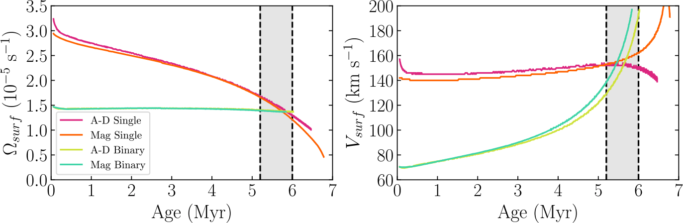
Binary star models are shown in Fig. 1 (columns 3&4). Not only the models do not reproduce the $k_2$ at $R_\star$ – even with large $\alpha_{\mathrm{ov}}$ – but also they are worse at reproducing the position in the HR diagram. If the single star models are apparently better at reproducing the current properties of the stars, it is because we chose $v_{\mathrm{ini}}$ such that $v_{\mathrm{surf}} (R_\star) = v_{\mathrm{surf},\star}$. During its evolution, a single star model sees its surface angular velocity $\Omega_{\mathrm{surf}}$ decrease and its radius increase in time; Its $v_{\mathrm{surf}}$ is thus constant in time (Fig. 2). In reality, the star has a companion. Its $\Omega_{\mathrm{surf}}$ is fixed by the orbital motion (the binary is pseudo-synchronised) while its radius is increasing in time. Its $v_{\mathrm{surf}}$ thus increases in time (Fig. 2). Compared to a single star model, a binary star model has lower $\Omega_{\mathrm{surf}}$ and $v_{\mathrm{surf}}$ throughout its lifetime until reaching $R_\star$, thus has been less mixed during its evolution. Consequently, a binary model has a larger $k_2$ when reaching $R_\star$ than its single-star counterpart. The conclusion is not that the single star models are better are reproducing the stellar properties, but that it is important to take into account the binary interactions by computing binary models. Yet, something is missing in the binary models to reproduce the stellar properties. We investigate several possibilities hereafter.

Figure 2.

Evolution of $\Omega_{\mathrm{surf}}$ and $v_{\mathrm{surf}}$ with time for single and binary models.

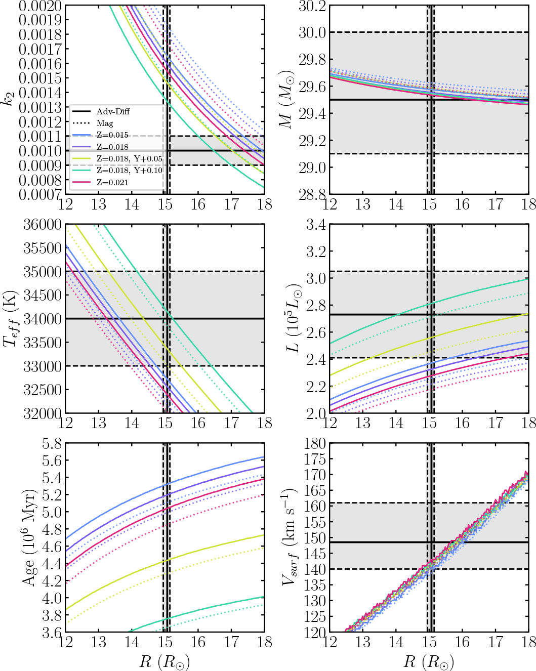
Could it be the metallicity or initial helium abundance? We tested the influence of the metallicity and the initial He abundance on the models. We varied Z within its error bars: an increase in Z leads to a decrease in $k_2$ but also a decrease in $T_{\mathrm{eff}}$ and L (Fig. 3). Yet, the impact is very limited. An increase in He leads to a decrease in $k_2$ and an increase in $T_{\mathrm{eff}}$ and L (Fig. 3). While it solves partially the problem, it is not supported observationally.

Figure 3.

Evolution of stellar parameters with R for binary models with different Z and He.

Could it be the mass-loss rate? Winds are clumped, and if clumping starts close to the photosphere, theoretical mass-loss rates are underestimated by a factor $f^{0.25}$, with $f = 8-10$ (Krtička et al. Reference Krtička, Kubát and Krtičková2024). We computed stellar models with Krtička et al. (Reference Krtička, Kubát and Krtičková2024) mass-loss rate multiplied by 1.8Footnote ². The models have a slightly larger $M_{\mathrm{ini}} = 32.0 M_{\odot}$, thus slightly larger $T_{\mathrm{eff}}$ and L at $R_\star$ (Fig. 4). Yet, $k_2$ does not change compared to non-clumped models and the $k_2$-discrepancy is still not solved. The reason is that the star is initially slightly more massive so its $k_2$ decreases faster. However, it reaches $R_\star$ earlier thus has not had time to evolve as much as the non-clumped models. Its density contrast is not as pronounced, which compensates the faster decrease in $k_2$. In conclusion, even if mass-loss rate is underestimated, it has no significant impact on the models.

Figure 4.

Evolution of stellar parameters with R for binary models with larger mass-loss rate.

Figure 4 Long description

Panel A: A line graph shows the evolution of k2 with R (R☉). The x-axis is labeled R (R☉) ranging from 12 to 18, and the y-axis is labeled k2 ranging from 0.0007 to 0.0020. Different lines represent various models: Adv-Diff, Mag, Standard with αov = 0.5 and 0.8, and Clumped with αov = 0.5 and 0.8. Panel B: A line graph shows the evolution of M (M☉) with R (R☉). The x-axis is labeled R (R☉) ranging from 12 to 18, and the y-axis is labeled M (M☉) ranging from 28.8 to 30.2. Different lines represent various models. Panel C: A line graph shows the evolution of Teff (K) with R (R☉). The x-axis is labeled R (R☉) ranging from 12 to 18, and the y-axis is labeled Teff (K) ranging from 32000 to 36000. Different lines represent various models. Panel D: A line graph shows the evolution of L (10^5 L☉) with R (R☉). The x-axis is labeled R (R☉) ranging from 12 to 18, and the y-axis is labeled L (10^5 L☉) ranging from 2.0 to 3.4. Different lines represent various models. Panel E: A line graph shows the evolution of Age (10^6 Myr) with R (R☉). The x-axis is labeled R (R☉) ranging from 12 to 18, and the y-axis is labeled Age (10^6 Myr) ranging from 4.4 to 6.6. Different lines represent various models. Panel F: A line graph shows the evolution of Vsurf (km s^-1) with R (R☉). The x-axis is labeled R (R☉) ranging from 12 to 18, and the y-axis is labeled Vsurf (km s^-1) ranging from 120 to 180. Different lines represent various models.

4. GENEC models put to the $\mathbf{k_2}$-test: Status quo

With the best up-to-date physics included, GENEC models do show the $k_2$ discrepancy for HD 152248. The standard binary models predict too low $T_{\mathrm{eff}}$ and L but too high a $k_2$. Only an increase in $\alpha_{\mathrm{ov}}$ allows the models to get closer to reproduce the observations. A change in the metallicity has a non-significant impact on the models. An increase in the initial He abundance allows to better reproduce the observations; It is however not observationally supported. Clumped binary models with larger mass-loss rates slightly improve on $T_{\mathrm{eff}}$ and L predictions – mostly because $M_{\mathrm{ini}}$ is larger. Yet, the impact on $k_2$ is non-significant. Therefore, even if the mass-loss rate of our standard models is underestimated, it has no impact on our conclusions that models predict too high a $k_2$. In summary, our investigations suggest that we need a mechanism that slows down the stellar radius increase in time. In the future, we will increase by an order of magnitude the number of binaries studied this way in a wide range of stellar and orbital parameters.