
1. Introduction
In many natural and industrial situations, relatively heavy fluid is continuously introduced at the base of a porous medium. The importance of this situation has led to a whole series of laboratory experiments being undertaken to simulate such occurrences. Recently there has been an additional series of papers and laboratory experiments by authors from different groups motivated by the societally important problem of carbon sequestration, the final part of carbon capture and storage (e.g. Huppert & Neufeld Reference Huppert and Neufeld2014). To mitigate the effects of global warming, attributed to the current anthropogenic annual worldwide emission of 43 billion tonnes of carbon dioxide ( $\textrm {CO}_2$), numerous groups around the world are evaluating how to store super-critical, liquid-like,
 $\textrm {CO}_2$ at depths in excess of 800 m (roughly the depth associated with the pressure and temperature needed to compress
 $\textrm {CO}_2$ to the super-critical state). The
 $\textrm {CO}_2$ is relatively less dense than the surrounding interstitial brine and so it rises like a buoyant plume until it encounters a relatively impermeable cap rock and spreads beneath it as a gravity current in a porous medium (Bickle Reference Bickle2009). There are other situations in the Earth where dense fluids discharge into regions containing lower density interstitial fluids in permeable geological media. An important example occurs during discharges of high temperature fluids from magma chambers. These flows can cause discharges of gases at volcanoes and are associated with the formation of metalliferous ore deposits (Afanasyev et al. Reference Afanasyev, Blundy, Melnik and Sparks2018). While the overall density of the fluids is less than the surrounding ground waters, they characteristically exsolve dense brines, which can separate and then displace surrounding fresh water in the permeable crust.
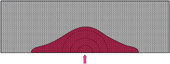
The focus of the present paper is to analyse the evolution resulting from the injection of relatively heavy fluid at the base of a semi-infinite porous medium (shown schematically in figure 1). We show that the flow first spreads in the form of a hemisphere of steadily increasing radius  $r_N(t)\propto t^{1/3}$, where
 $t$ is time, with no dependence on the permeability of the medium nor viscosity of the fluid. This regime can be distinguished from the more familiar thin-layer theory, which instead predicts that
 $r_N(t)\propto t^{1/2}$, with a prefactor dependent on the permeability of the medium, the viscosity of the fluid and the density difference between the intruding and interstitial fluids (Lyle et al. Reference Lyle, Huppert, Hallworth, Bickle and Chadwick2005). During the hemispherical regime, buoyancy, and hence the density difference, as well as the viscosity and permeability of the medium, are irrelevant. After a progression of intrinsic time scales that we determine, the hemispherical regime transitions towards the axisymmetric thin-layer regime with radius
 $r_N(t)\propto t^{1/2}$. The work of Lyle et al. (Reference Lyle, Huppert, Hallworth, Bickle and Chadwick2005) and others addressing fluid injection into porous media have focussed on this final thin-layer regime, and various generalisations, in which stresses become hydrostatic to leading order under the Dupuit approximation (Bear Reference Bear1972). These generalisations include, in particular, an allowance for vertical confinement in both axisymmetric and two-dimensional configurations (Nordbotten & Celia Reference Nordbotten and Celia2006; Pegler, Huppert & Neufeld Reference Pegler, Huppert and Neufeld2014; Zheng et al. Reference Zheng, Guo, Christov, Celia and Stone2015; Guo et al. Reference Guo, Zheng, Celia and Stone2016). The analysis of regimes that do not satisfy the thin-layer approximation and their role as a transient asymptotic regime, the focus of the present paper, has received less attention.
The response to an input flux of heavy viscous fluid into a porous medium above an impermeable horizontal boundary.

The significance of transitions connecting non-hydrostatic regimes due to a point injection and thin-layer gravity currents has been discussed previously in the context of a viscous fluid layer introduced into a vertical Hele-Shaw cell (Pegler et al. Reference Pegler, Kowal, Hasenclever and Worster2013). By applying a scaling analysis, an intrinsic length scale describing the transition was formulated and found to correlate with the magnitude of deviations between the experimental observations and the predictions of an associated thin-layer theory (focusing on the time for the current to reach a given thickness). Corresponding dimensionless numbers have been applied to measure the relative importance of non-hydrostatic effects from a point injection in porous media (Pegler et al. Reference Pegler, Huppert and Neufeld2014, Reference Pegler, Maskell, Daniels and Bickle2017), and determined to correlate with deviations between experimental observations and thin-layer modelling.
The present paper develops predictions for a series of time scales on which the initially radial flow from a localised point or line source transitions to a corresponding thin-layer regime in both axisymmetric and two-dimensional geometries. We demonstrate the transition explicitly in the laboratory by showing a consistent collapse of the results of a series of experiments onto an evolution (universal subject to scaling) connecting the radially flowing regime near the source to the gravity-current regime in the two-dimensional case.
We begin in § 2 by considering the initial response of an expanding hemisphere in an axisymmetric geometry. Using just conservation of volume, we present the form of the initial motion. By utilising the expressions for the pressure and dimensions of the current in this regime in conjunction with existing predictions describing the evolution of the final thin-layer regime from the study of Lyle et al. (Reference Lyle, Huppert, Hallworth, Bickle and Chadwick2005), we obtain a series of time scales on which four different properties of the flow – horizontal length, height, aspect ratio and ratio of gravitational to viscous stresses – transition from the hemispherical regime to the thin-layer axisymmetric regime. In § 3, we address the corresponding two-dimensional transition in a porous medium or Hele-Shaw cell. The transition in the two-dimensional case is demonstrated experimentally in § 4, showing a consistent collapse with no fitting parameters to a trajectory spanning the radial regime to the gravity-current regime, with good agreement in the two limits. Finally, in § 5 we discuss briefly how to extend our results to flows in some vertically heterogeneous porous media, and present a somewhat dramatic experimental photograph of how a relatively permeable upper layer can be in a very different flow regime from a relatively less permeable lower layer. We end the paper in § 6 with a brief summary.
2. Axisymmetric injection from hemisphere to gravity current
We consider the injection of incompressible fluid at the base of a porous medium, as illustrated schematically in figure 1. We model the flow using Darcy's law (Bear Reference Bear1972) with the condition of incompressibility,
 \begin{gather} \mu {\boldsymbol{u}}/k ={-}\boldsymbol{\nabla} p -\rho {\boldsymbol{g}}, \end{gather}
 \begin{gather}\boldsymbol{\nabla} \boldsymbol{\cdot} \boldsymbol{u} = 0 , \end{gather}
where  $\mu$ is the dynamic viscosity of the fluid, k is the permeability of the medium,
 $p$ is pressure,
 ${\boldsymbol {g}}$ is the acceleration due to gravity and
 $\boldsymbol {u}$ is the Darcy velocity. As an overview of the proceeding analysis, we begin by deriving, using just mass conservation (2.2), the form of the flow near the point of injection. By reference to the force balance equation (2.1), we argue that, due to the large pressures arising near the point source, gravity is initially negligible in this regime. Following this, we recall the solutions describing the thin-layer regime arising at late times in which the vertical component of (2.1) exhibits a leading-order balance between the pressure and gravitational terms (Lyle et al. Reference Lyle, Huppert, Hallworth, Bickle and Chadwick2005). By then considering the predictions of the two regimes in regards to the dimensions of the flow and the relative importance of gravitational to viscous terms, we present a series of predictions for the time scales on which differing properties of the first regime transition to the second.
2.1. Initial hemispherical regime
For a point source of fluid fed radially at a constant volumetric flux  $Q$, conservation of volume dictates that the radius of the injected fluid,
 $a(t)$, satisfies
 \begin{equation} \frac{2}{3} {\rm \pi}\phi a^3=Qt \quad \textrm{or} \quad a(t)= \left (\frac{3Q}{2{\rm \pi} \phi}\right )^{1/3}t^{1/3}, \end{equation}
where  $\phi$ is the porosity of the medium. By differentiating this expression, it follows that the front of the injected fluid propagates at a speed of
 \begin{equation} \dot a=(Q/18{\rm \pi} \phi)^{1/3}t^{{-}2/3}. \end{equation}
By mass conservation (2.2), the Darcy velocity  $\boldsymbol {u}$ satisfies
 \begin{equation} {\boldsymbol u}(r,t)= \phi \dot a a^2 \hat{\boldsymbol{r}}/r^2=Q\hat{\boldsymbol{r}}/(2{\rm \pi} r^2), \end{equation}
where  $r$ is a (spherical) radial coordinate and
 $\hat {\boldsymbol {r}}$ is the unit vector in the radial direction. The equation above predicts that the velocity field diverges near the point of injection (
 $u \to \infty$ as
 $r \to 0$). Therefore, since the gravitational body force on the right-hand side of (2.1) is constant, the viscous stress will be much greater than the gravitational force sufficiently close to the injection point. At sufficiently early times, gravity is therefore negligible. By substituting the Darcy velocity (2.5) into (2.1) and integrating the resulting equation with respect to
 $r$, we obtain the corresponding pressure field
 \begin{equation} p = \frac{\mu \phi a^2 \dot a}{kr} + p_0 = \frac{\mu Q}{2{\rm \pi} k r} + p_0, \end{equation}
independent of time, where  $p_0$ is a constant reference pressure. Again, we see that the pressure gradient will greatly exceed the hydrostatic (gravitational) pressure gradient,
 $\rho g$, in the limit
 $r \to 0$. In summary, during this regime in which gravity is unimportant, both the horizontal and vertical dimensions of the current are given to leading order by (2.3), with
 \begin{equation} r_N(t) \sim h(0,t) \sim a(t) = \left (\frac{3Q'}{2{\rm \pi}}\right )^{1/3}t^{1/3} \quad (t \to 0), \end{equation}
where  $Q'=Q/\phi$. We can anticipate that this regime is stable if the injected fluid is more viscous than the ambient fluid, in correspondence with the criterion for Saffman–Taylor instability (Saffman & Taylor Reference Saffman and Taylor1958).
2.2. Late-time axisymmetric thin-layer regime
The theoretical development for a thin-layer gravity current follows the alternative assumption that the vertical stress balance in (2.1) is dominated by the pressure gradient and buoyancy, such that  $\partial p/\partial z \sim -\rho g$ is hydrostatic to leading order. Following this assumption, one can reduce the evolution of the flow to a nonlinear diffusion equation and solve it using similarity theory (Barenblatt Reference Barenblatt1996). In the case of an axisymmetric current introduced centrally at a constant flux, the following relationships have been determined for the radius and height profile of the current in the thin-layer regime (Lyle et al. Reference Lyle, Huppert, Hallworth, Bickle and Chadwick2005),
 \begin{gather} r_N(t)=1.16(\beta Q')^{1/4}t^{1/2}, \end{gather}
 \begin{gather}h(r,t) = (Q'/\beta)^{1/2}\varPhi [r/r_N(t)] \approx 0.67(Q'/\beta)^{1/2}(1-r/r_N), \end{gather}
where  $\varPhi (y)$ is an approximately linear function derived from the leading-order solution near the nose, and
 $\beta =\Delta \rho gk/\phi \mu$ is the buoyancy speed.
While the linear profile of (2.8b), derived by extrapolating the solution near the nose through the length of the current, provides an excellent approximation for the overall shape (see figure 8 of Lyle et al. Reference Lyle, Huppert, Hallworth, Bickle and Chadwick2005), the height profile determined by thin-layer theory,  $h(r,t)$, instead exhibits an unphysical logarithmic singularity as
 $r \to 0$ (Lyle et al. Reference Lyle, Huppert, Hallworth, Bickle and Chadwick2005). By contrast, the height profile in reality and predicted by (2.7) is finite. The introduction of vertical velocities near the point injection, incorporated in (2.7), therefore acts to regularise this singularity in the height profile.
Using the prediction of (2.8b) to approximate the height scale, we obtain
 \begin{equation} h(0,t)=0.67 \, (Q'/\beta)^{1/2}. \end{equation}
Combining this with (2.8a), we obtain the approximation for the aspect ratio in the thin-layer regime,
 \begin{align} \gamma (t) &= h(0,t)/r_N(t) \end{align}
 \begin{align} &= 0.58\, (Q'/\beta ^3)^{1/4}t^{{-}1/2}. \end{align}
This result predicts a progressively decreasing aspect ratio, consistent with the strengthening of the thin-layer assumption with time. Conversely, it predicts that  $\gamma \to \infty$ for small times, thereby predicting a loss of asymptotic consistency in the thin-layer approximation. This conclusion is in agreement with the transition of the flow from an early-time regime in which vertical velocities are significant.
2.3. Intrinsic scales
For the purpose of formulating general expressions describing the regime transitions, we recast the results in terms of intrinsic scales. On the basis of scaling, we can determine the unique intrinsic time and length scales of the system
 \begin{equation} T=(Q'/\beta ^3)^{1/2}\quad \textrm{and}\quad L=(Q'/\beta)^{1/2}, \end{equation}
respectively. In terms of these, the frontal evolution in the radial regime (2.7) reads
 \begin{equation} a/L=(3/2{\rm \pi})^{1/3}(t/T)^{1/3}. \end{equation}
For the thin-layer regime, the equations describing the evolution of the horizontal extent (2.8b), height (2.9) and aspect ratio (2.11), become
 \begin{gather} r_N/L = 1.16 \, (t/T)^{1/2}, \end{gather}
 \begin{gather}h(0,t)/L = 0.67, \end{gather}
 \begin{gather}\gamma = 0.58 \, (t/T)^{{-}1/2}, \end{gather}
respectively.
As a metric to measure the transition from a regime affected by the injection pressures to one dominated by hydrostatic pressure, we can consider the ratio of buoyancy,  $\Delta \rho g$, to viscous stresses,
 $\mu u/k$, in (2.1), as
 \begin{equation} A(t)= \Delta \rho g k/\mu u. \end{equation}
Dimensionless numbers of this form have been proposed previously (Pegler et al. Reference Pegler, Kowal, Hasenclever and Worster2013, Reference Pegler, Huppert and Neufeld2014, Reference Pegler, Maskell, Daniels and Bickle2017) and used to represent the relative significance of stresses due to fluid injections compared with the hydrostatic pressure. Substituting  $u(a,t)$ given by (2.5) into (2.17), we determine the characteristic value of
 $A$ at the flow front of the radial regime,
 $A_1(t)$, as
 \begin{align} A_1(t) &= 2 {\rm \pi}(\beta /Q')a^2 \nonumber\\ &= (18 {\rm \pi})^{1/3} \beta Q'^{{-}1/3}t^{2/3} \nonumber\\ &= (18{\rm \pi})^{1/3} (t/T)^{2/3}, \end{align}
where we have made use of (2.3) and (2.12b) to evaluate  $a(t)$ and
 $T$, respectively. The increase of
 $A_1$ as
 $t^{2/3}$ is consistent with the reduction in velocity at the flow front, and the increasing importance of gravity, as it extends from the source.
For the thin-layer regime, the characteristic value of  $u$ at the flow front is given from (2.8a) by
 \begin{align} u &= 0.58 \phi (\beta Q')^{1/4}t^{{-}1/2} \nonumber\\ &= 0.58 \phi LT^{{-}1}(t/T)^{1/2}. \end{align}
Substituting the above into (2.17), we obtain the ratio of buoyancy to viscous stresses at the nose of the current during the thin-layer regime,
 \begin{align} A_2(t) &= 1.72 \, (\beta^3/Q')^{1/4}t^{1/2} \nonumber\\ &= 1.72 \, (t/T)^{1/2}. \end{align}
Since the flow rate at the front of the thin layer decreases with time, the relative importance of buoyancy is again predicted to become more important with time in this regime, reflected by the increase of  $A_2$ as
 $t^{1/2}$ given above, consistent with a transition towards gravity-driven flow.
2.4. Transition times
By equating the asymptotic expressions for the early- and late-time regimes derived in § 2.1 and 2.2, we can derive a series of time scales on which the transition between the two regime occurs as follows. To begin, by equating the predictions for the ratio of viscous to buoyancy forces  $(A_1=A_2)$ given by (2.18) and (2.20), we obtain, on simplification,
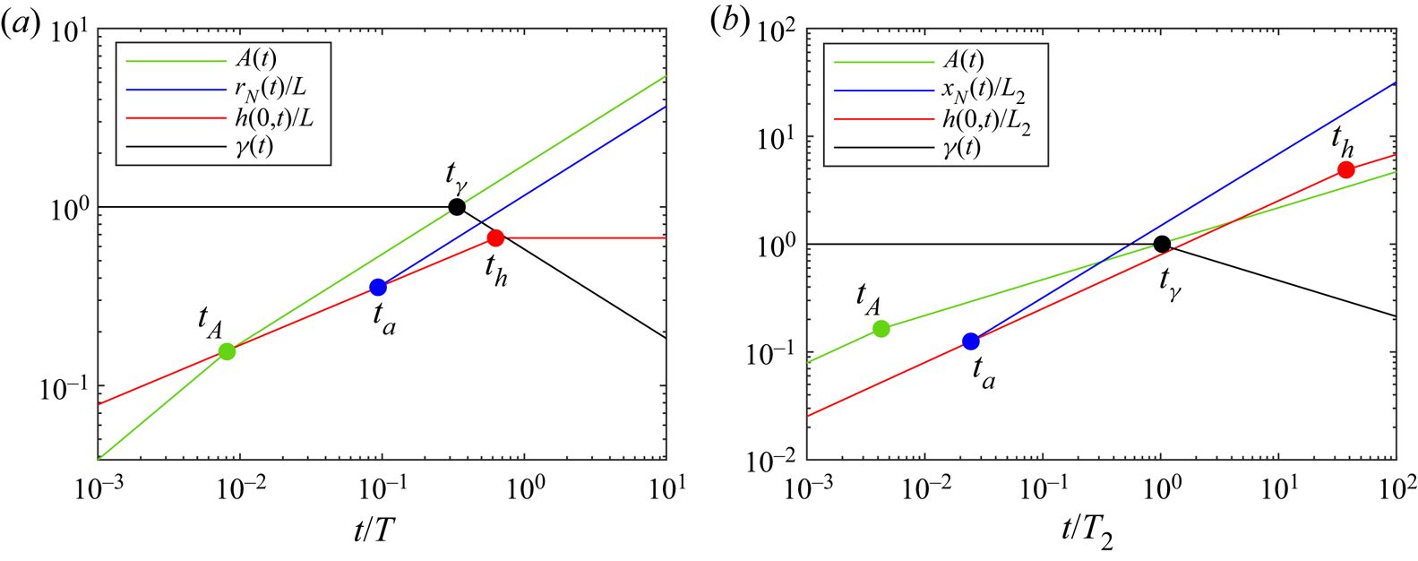
 \begin{equation} t_A/T=0.0081, \end{equation}
at which time  $a/L=h/L=0.16$. Gravity therefore begins to become important at less than one hundredth of the time scale
 $T$ with a transition that occurs well before
 ${A_2=1}$. A different time for transition,
 $t_r$, may be defined by equating the predictions for the position of the flow fronts,
 $a(t_r)=r_N(t_r)$, given by (2.13) and (2.14), yielding
 \begin{equation} t_r/T=0.094, \end{equation}
at which time  $a/L=h/L=0.36$. This result indicates that, as far as the horizontal extent of the current is concerned, the flow begins to switch between the regimes at approximately 10 % of
 $T$. Additionally, we could consider the transition time,
 $t_\gamma$ defined by
 $\gamma (t_\gamma )=1$, where
 $\gamma$ is given by (2.16), which leads to
 \begin{equation} t_\gamma/T=0.34, \end{equation}
at which time  $a/L=R/L=0.54$. Finally, we evaluate the time
 $t_h$ at which the height of the current at the input takes the same value in the relationships for the two different regimes, (2.13) and (2.15), as
 \begin{equation} t_h/T=0.63,\end{equation}
at which time  $r_N/L=0.92$ and
 $h/L=0.67$. By comparing this with (2.22), we see that the transition time for the thickness takes relatively longer than the time scale of transition for the horizontal scale. We attribute this to the fact the vertical flow front lies considerably closer to the source input, implying that the impact of the non-hydrostatic source conditions on the flow has a significant influence to longer times.
Plots showing the predictions for  $A(t), h/L, r_N/L$ and
 $\gamma$ in the early-time regime, given by (2.13), and in the late-time regime, given by (2.14)–(2.16), are shown as functions of time in figure 2(a). The plot illustrates the differing times (marked by filled circles) on which the different properties of the flow switch from the predictions of the radial regime to those of the gravity current.
(a) Plots of the predicted asymptotes for  $A$ (green),
 $r_N(t)$ (blue),
 $h(0,t)$ (red) and
 $\gamma (t)=h(0,t)/r_N$ (black) for the initial and final responses in an axisymmetric situation (§ 2). The times where the curves meet, indicated by filled circles, represent the characteristic times at which the flow switches its properties from one regime to the other, as determined in § 2.4. (b) As above, but for a two-dimensional geometry (§ 3).

2.5. Illustrative evaluation of time scales
To get a feel for the various time scales in experimental and geological contexts, we present values in table 1 using illustrative laboratory and geological values. Here, we use  $\Delta \rho / \rho \sim 0.01$ and
 $\nu = 10^{-6}\ \textrm {cm}^2\ \textrm {s}^{-1}$, which typifies aqueous solutions of sodium chloride at low concentrations. It should be noted that much larger ranges of densities, viscosities and injection fluxes across different geological contexts, encompassing liquids, gases and supercritical fluids, are possible; the evaluations here nonetheless illustrate the considerable variations arising across different rock types and laboratory conditions. The illustrative values in the geological cases in the first two rows represent typical values for low and high porosity rock (e.g. Kampman et al. Reference Kampman2014). The comparison between these two cases shows a variation in time scales of the order of a few months to tens of thousands of years.
Illustrative evaluations of the time scales on which the axisymmetric transition from radial to thin-layer regimes occurs, given by (2.21)–(2.24), for a selection of geological parameters and those of the experimental configuration of Lyle et al. (Reference Lyle, Huppert, Hallworth, Bickle and Chadwick2005). The values of the time scales for geological cases (first two rows) are given in years, while those of the experiment are given in seconds. To evaluate  $T$ using (2.12a,b), we have used the illustrative values of
 $\Delta \rho /\rho =0.01$ and
 $\nu =10^{-6}\ \textrm {m}^2\ \textrm {s}^{-1}$, which can characterise injections of slightly salty water (the solution with least concentration used in Lyle et al. Reference Lyle, Huppert, Hallworth, Bickle and Chadwick2005) and hydrothermal fluids, for example. Much larger ranges of density differences, viscosities and injection fluxes can occur across different geological contexts, encompassing liquids, gases and supercritical fluids; the evaluations here serve to illustrate the possibility for considerable variations arising across different rock types and laboratory conditions alone. The illustrative values for
 $\phi$ and
 $k$ in the geological context typify high porosity rock, such as sandstone, and low porosity rock, such as mudstone (e.g. Kampman et al. Reference Kampman2014).

The value for the laboratory ( $\Delta \rho / \rho \sim 0.01$) corresponds to the aqueous solutions of sodium chloride with least concentration used by Lyle et al. (Reference Lyle, Huppert, Hallworth, Bickle and Chadwick2005), which would have created the longest transitional time scale
 $T$ in their study. The time scales for this axisymmetric experiment are so short (<1 s) that the first (hemispherical) regime would have occurred primarily before the first measurements of the lengths of the currents were recorded. The intrinsic time scales for the two-dimensional situation, as characterised by our experiments presented in § 4 below (table 2), are longer (20–540 s), allowing us to monitor the evolution directly from the initiation of the input.
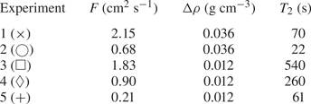
Parameter values used in our experiments of § 4.

3. Two-dimensional injection
The consideration of injection into a two-dimensional porous medium or a vertical Hele-Shaw cell leads to a similar exposition, although it differs quantitatively from the axisymmetric situation. The description will hence be relatively brief.
In the initial stages, when gravitational effects are irrelevant, conservation of volume dictates that
 \begin{equation} \tfrac{1}{2} {\rm \pi}a^2=F't, \end{equation}
forming the two-dimensional analogue of (2.3), where  $F$ is the constant two-dimensional input rate and
 $F'=F/\phi$. With length and time scales of
 \begin{equation} L_2=F'/\beta \quad \textrm{and} \quad T_2=F'/\beta ^2, \end{equation}
(3.1) becomes
 \begin{equation} a(t)/L_2=(2/{\rm \pi})^{1/2}(t/T_2)^{1/2}. \end{equation}
For the corresponding thin-layer regime in two dimensions, we quote (4.14), (4.15) and (4.17) of Huppert (Reference Huppert1986) and (3.13) of Huppert & Woods (Reference Huppert and Woods1995), which give the length, height and aspect ratio of the current as
 \begin{gather} x_N(t)/L_2 = 1.48 \, (t/T_2)^{2/3}, \end{gather}
 \begin{gather}h(0,t)/L_2 = 1.46 \, (t/T_2)^{1/3}, \end{gather}
 \begin{gather}\gamma = 0.99 \, (t/T_2)^{{-}1/3}, \end{gather}
respectively, when recast in terms of (3.2a,b). On using (3.3) and (3.4) to determine the characteristic Darcy velocity at the flow front in the two regimes using  $u = \phi \dot a$ and
 $u = \phi \dot x _N$, respectively, we determine the corresponding ratios of buoyancy to viscous stresses in the first (radial) regime and second (gravitational) regimes as
 \begin{gather} A_1(t) = (2{\rm \pi})^{1/2} (t/T_2)^{1/2}, \end{gather}
 \begin{gather}A_2(t) = 1.01 \, (t/T_2)^{1/3}, \end{gather}
respectively. Both of these expressions indicate that  $A$, and hence the relative importance of gravity, increases with time.
As for the axisymmetric case, we can similarly define a series of time scales on which the early-time regime with frontal position and height given by (3.3), with aspect ratio  $\gamma = 1$, transitions to the late-time gravity-current regime with dimensions and aspect ratio given by (3.4)–(3.5). Proceeding as in § 2.4, we equate the predictions in the two regimes [
 $A_1(t_A) = A_2(t_A)$,
 $a(t_x) = x_N(t_x)$,
 $\gamma (t_\gamma ) = 1$ and
 $a(t_h) = h(0, t_h)$], to determine a progression of transition times for the two-dimensional case
 \begin{gather} t_A/T_2 = 0.0043, \end{gather}
 \begin{gather}t_x/T_2 = 0.025, \end{gather}
 \begin{gather}t_\gamma/T_2 = 1.03, \end{gather}
 \begin{gather}t_h/T_2 = 37.5. \end{gather}
We note the considerably wider range of these time scales (spanning five orders of magnitude) in comparison with their axisymmetric counterparts. Thus, while qualitatively the results for the axisymmetric and two-dimensional geometries are similar, quantitatively, the differences in time scales are substantial.
4. Experimental analysis
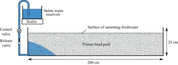
We conducted a series of laboratory experiments in a narrow acrylic tank of length 200 cm, height 25 cm and width 1 cm (figure 3). The tank was filled with glass beads of diameter 2 mm (figure 4), creating a porous medium of porosity  $\phi \approx 0.38 \pm 0.01$ and permeability
 $k\approx (3.1 \pm 0.2) \times 10^{-5}\ \textrm {cm}^{-2}$. These values correspond to those measured for 2 mm beads (Acton, Huppert & Worster Reference Acton, Huppert and Worster2001) and tested previously for this geometry (Pegler et al. Reference Pegler, Huppert and Neufeld2014). The medium was saturated with approximately fresh water with a density of
 $0.999\ \textrm {g}\ \textrm {cm}^{-3}$. Densities were measured using an oscillating U-tube density meter to an accuracy of
 $10^{-6}\ \textrm {g}\ \textrm {cm}^{-3}$. In order to provide conditions favouring the persistence of the early-time radial regime, small density differences between the injected and ambient fluids were used. Thus, for the injected fluid, we used solutions of salty water with densities varying from 1.011 to
 $1.035\ \textrm {g}\ \textrm {cm}^{-3}$, which were dyed with blue food colouring. The kinematic viscosity
 $\nu \approx 0.010 \pm 0.001\ \textrm {cm}^2\ \textrm {s}^{-1}$ was measured using a U-tube viscometer. The solutions were introduced into the medium through an inlet located at the bottom left-hand corner of the cell. A siphon of rubber tubing connected the inlet to a raised reservoir of salty water, and the release of fluid was initiated using an intermediary ball valve. The evolution of the flow was recorded using a digital SLR camera, which took photographs at regular intervals of 1 or 5 s. The rate of input was determined by measuring the weight of the reservoir over the course of each experiment.
Schematic of our experimental apparatus.

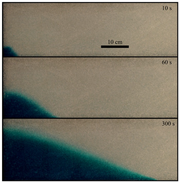
A progression of photographs showing experiment 2 (green circles in figure 5) at times  $t = 10$, 60 and 300 s. The progression illustrates the transition from an initial regime of approximately radial flow in the vicinity of the injection at the bottom left-hand corner (with an aspect ratio comparable to unity,
 $\gamma \approx 1$) towards an increasingly slender gravity current with increasing time.

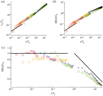
Collapsed experimental data showing (a) the horizontal length of the current,  $x_N(t)$, scaled by the length scale
 $L_2$ defined by (3.2a,b), (b) the height above the input point,
 $h(0,t)$, scaled by
 $L_2$ and (c) the aspect ratio of the current
 $\gamma$ (height over length) as functions of dimensionless time
 $t/T_2$, where
 $T_2$ is the time scale (3.2a,b). The symbols denoting the experiments are given in table 2. The early-time predictions for
 $x_N/L_2$ and
 $\gamma$ associated with the radial regime (3.3), and the late-time predictions associated with gravity-current regime (3.12) are shown as solid black lines. No fitting parameters have been used in formulating this collapse.

The parameter values used are shown in table 2. The main parameter varied was the volumetric rate of input per unit width  $F$, which spanned an order of magnitude from 0.2 to
 $2\ \textrm {cm}^2\ \textrm {s}^{-1}$. The evolutions of the frontal position
 $x_N(t)$, height of the current at the source,
 $h(0,t)$ (each scaled by
 $L_2$), and the aspect ratio, measured digitally from the photographs, are shown in figure 5(a–c). A progression of photographs showing the evolution of experiment 2 is presented in figure 4, illustrating the transition of the shape of current from an aspect ratio comparable to unity towards the shallower aspect ratio characteristic of a gravity current. Figure 5(c) plots
 $\gamma = h(0,t)/x_N(t)$, the ratio of the height of the current above the source to its horizontal extent. Overlaid are the early- and late-time predictions of (3.3) and (3.12). The observations indicate that the experiments undergo transitions from a regime approximating a radial flow (with aspect ratio
 $\gamma \approx 1$) to that of the gravity current
 $\gamma \sim (t/T_2)^{-1/3} \to 0$. Each experiment was terminated once the current reached the free surface of the ambient water. Therefore, different experiments cover different intervals of the same collapsed theoretical transition.
The experiments show a characteristic collapse to a consistent trajectory spanning the early-time radial flow to the late-time gravity current in accordance with the intrinsic scales. However, we observe consistent overshoots of the experimental predictions for the frontal and height positions,  $x_N(t)$ and
 $h(0,t)$, at early times, as compared with the theoretical prediction (2.13). We attribute this to the effect of hydrodynamic dispersion, which causes the front of the fluid layer to become diffuse, as can be observed in figure 4. To conserve mass, the smeared front must therefore extend slightly further ahead than would apply in the case of the ideal sharp interface assumed in the theory. At early times, there is a similar 20 % overshoot in both vertical and horizontal dimensions, which is consistent with dispersion initially playing a similar role in both directions during the radial regime. In view of its lower density, the dispersed fluid lingers preferentially above the source, producing a transition from a smeared interface upstream to a sharper interface near the nose. This is in agreement with the general form of stratified gravity currents containing a distribution of densities (Pegler, Huppert & Neufeld Reference Pegler, Huppert and Neufeld2016).
The comparison between the observations and the theoretical predictions also reveals scatter in the evolution of the flow fronts at early times, particularly shown in the evolution of the aspect ratio  $\gamma$ (figure 5c). This is likely caused by the sensitivity of the early-time flow to the inhomogeneities in the permeability of the bead pack (some associated roughness in the profile of the flow front is evident in the early-time flow front shown in the first image of figure 4).
We also observe that, while the horizontal flow front has converged appreciably to the late-time prediction by  $t/T_2 = 1$ (figure 5a), the height and aspect ratio transition relatively slower towards their respective thin-layer predictions (figure 5b,c). This variation in transitional time scales is consistent with our findings of § 3 showing that the transition time for the horizontal extent is faster than the vertical. As noted there, this is likely because the height is affected by the near-field effects of the injection more so than the horizontal extent, which is primarily affected by the gravity-driven flow that establishes far from the injection point.
5. Vertically varying permeability and porosity
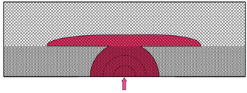
In the Earth there can be considerable variations in permeability and porosity in both vertical and horizontal directions. Analysis of these configurations has been incorporated in the context of thin-layer theory (e.g. Huppert & Woods Reference Huppert and Woods1995; Zheng et al. Reference Zheng, Soh, Huppert and Stone2013; Hinton & Woods Reference Hinton and Woods2018). Considering only vertical variations, we realise that it may be possible for an expansion in the approximately hemispherical regime to intrude into a region where the expansion can proceed more like a gravity current. A hypothetical sketch of this response in a two-layer system (with a much more permeable upper layer) makes up figure 6. To confirm the potential to transition between a regime with significant vertical velocities in the lower layer and a thin gravity current in the upper layer, we carried out a laboratory experiment in the extreme case of a porous layer topped by air in a cell of width 1 cm filled with glass ballotini of diameter 2 mm to a depth of 4 cm. An input of blue-dyed glycerine of viscosity  $7.5\ \textrm {cm}^2\ \textrm {s}^{-1}$ and density
 $1.26\ \textrm {g}\ \textrm {cm}^{-3}$ was fed at a rate of
 $0.18\ \textrm {cm}^2\ \textrm {s}^{-1}$ to the base of the container and photographs taken every 2 s.
The possible response in a two-layer system in which the porous medium in the upper section is considerably more permeable than in the lower section.

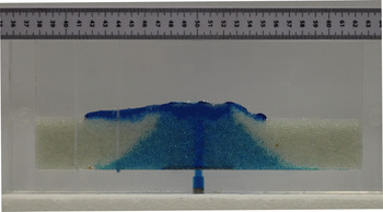
Following an initial radial spreading from the input position at the base of the cell, the current in the lower layer developed similarly to that shown in figure 4. Initially, it exhibited a rounded top and, subsequently, a wedge-shaped nose. By approximately 100 s, the flow was at the top of the layer (with some vertical uplift of the beads as the flow approached the interface, which perturbed the surface from being horizontal). By 140 s there was a fully developed horizontal flow along the interface (figure 7), which lengthened with time. Thereafter, parts of the heavy fluid sunk back into the porous layer in the form of broad fingers. This replicates motions seen in Acton et al. (Reference Acton, Huppert and Worster2001) and similarly in Bharath & Flynn (Reference Bharath and Flynn2021). There are similarities here to the configuration analysed by Huppert, Neufeld & Strandkvist (Reference Huppert, Neufeld and Strandkvist2013), who considered the conditions under which an input of relatively heavy fluid into the base of a two-layered porous medium flows into the upper layer because of its greater permeability.
The result of an experiment described in § 5 in a porous layer through which the fluid penetrates the air above and flows along the top of the layer as a gravity current.

6. Summary
We have evaluated, theoretically and experimentally, the response to the constant injection at a point source of a viscous fluid that is relatively more dense than the interstitial fluid of the surrounding porous medium. The medium lies above a rigid horizontal boundary and the source point is at that boundary. The analysis was presented for both axisymmetric and two-dimensional situations. We show that the fluid expands first hemispherically (or as a semi-disc in the two-dimensional situation), where gravity is negligible, and then transitions to a small-slope gravity current.
We demonstrated a wide range of different transition times between the early time spherically radial regime and the gravity current, dependent on which quantity is used to define the transition. Considering the ratio between viscous and gravitational forces, we determined that, for the fully three-dimensional, axisymmetric case, the transition time  $t_A/T=0.0081$ (0.0043 for the two-dimensional situation). Considering the horizontal radius of the resulting flow, we evaluated the transition time
 $t_a/T=0.093$ for axisymmetric situations (and 0.025 for the two-dimensional situation). Considering the height of the flow above the source point, we found that
 $t_h/T=0.63$ (37.5 for two-dimensional situations). Considering the slope, defined by the aspect ratio of height above the input to the horizontal radius at the boundary (the ratio of the two previous criteria),
 $t_\gamma /T=0.34$ (1.0 for two-dimensional situations). These large differences between the various time scales – a factor of approximately 80 in the axisymmetric situation and 9000 for the two-dimensional situation – are somewhat surprising. They show that different aspects of the flow become important at different times.
Because the overall time scale  $T$ is strongly dependent on the permeability (to the minus three halves in the axisymmetric situation, and to the minus one in the two-dimensional situation), we hypothesised that a lower, relatively impermeable layer may display significant vertical velocities controlled by the injection, while at the same time the flow penetrating into an upper, much more permeable layer could exist in a thin-layer regime. The potential for this to occur was demonstrated experimentally in figure 7, which shows the development of a thin gravity current in an upper, more permeable region that extends ahead of the fluid in the lower region.
Because the characteristic time scales we determine depend on parameters whose value is very different in illustrative laboratory settings and in the Earth, the relatively rapid transition to a gravity current – taking seconds to minutes in the laboratory – can take thousands of years in the Earth.
Acknowledgements
We thank M. Hallworth who helped with the experiment described in § 5. We are grateful to A. Rust and S. Sparks for helpful discussions during the initiation of this work. H.E.H. acknowledges support in the form of a Leverhulme Emeritus Fellowship.
Declaration of interests
The authors report no conflict of interest.