



%20--%3e%3c!DOCTYPE%20svg%20PUBLIC%20'-//W3C//DTD%20SVG%201.0//EN'%20'http://www.w3.org/TR/2001/REC-SVG-20010904/DTD/svg10.dtd'%3e%3csvg%20version='1.0'%20id='Layer_1'%20xmlns='http://www.w3.org/2000/svg'%20xmlns:xlink='http://www.w3.org/1999/xlink'%20x='0px'%20y='0px'%20width='64px'%20height='64px'%20viewBox='5.5%20-3.5%2064%2064'%20enable-background='new%205.5%20-3.5%2064%2064'%20xml:space='preserve'%3e%3cg%3e%3ccircle%20fill='%23FFFFFF'%20fill-opacity='0'%20cx='37.785'%20cy='28.501'%20r='28.836'/%3e%3cpath%20fill='%23595959'%20d='M37.441-3.5c8.951,0,16.572,3.125,22.857,9.372c3.008,3.009,5.295,6.448,6.857,10.314%20c1.561,3.867,2.344,7.971,2.344,12.314c0,4.381-0.773,8.486-2.314,12.313c-1.543,3.828-3.82,7.21-6.828,10.143%20c-3.123,3.085-6.666,5.448-10.629,7.086c-3.961,1.638-8.057,2.457-12.285,2.457s-8.276-0.808-12.143-2.429%20c-3.866-1.618-7.333-3.961-10.4-7.027c-3.067-3.066-5.4-6.524-7-10.372S5.5,32.767,5.5,28.5c0-4.229,0.809-8.295,2.428-12.2%20c1.619-3.905,3.972-7.4,7.057-10.486C21.08-0.394,28.565-3.5,37.441-3.5z%20M37.557,2.272c-7.314,0-13.467,2.553-18.458,7.657%20c-2.515,2.553-4.448,5.419-5.8,8.6c-1.354,3.181-2.029,6.505-2.029,9.972c0,3.429,0.675,6.734,2.029,9.913%20c1.353,3.183,3.285,6.021,5.8,8.516c2.514,2.496,5.351,4.399,8.515,5.715c3.161,1.314,6.476,1.971,9.943,1.971%20c3.428,0,6.75-0.665,9.973-1.999c3.219-1.335,6.121-3.257,8.713-5.771c4.99-4.876,7.484-10.99,7.484-18.344%20c0-3.543-0.648-6.895-1.943-10.057c-1.293-3.162-3.18-5.98-5.654-8.458C50.984,4.844,44.795,2.272,37.557,2.272z%20M37.156,23.187%20l-4.287,2.229c-0.458-0.951-1.019-1.619-1.685-2c-0.667-0.38-1.286-0.571-1.858-0.571c-2.856,0-4.286,1.885-4.286,5.657%20c0,1.714,0.362,3.084,1.085,4.113c0.724,1.029,1.791,1.544,3.201,1.544c1.867,0,3.181-0.915,3.944-2.743l3.942,2%20c-0.838,1.563-2,2.791-3.486,3.686c-1.484,0.896-3.123,1.343-4.914,1.343c-2.857,0-5.163-0.875-6.915-2.629%20c-1.752-1.752-2.628-4.19-2.628-7.313c0-3.048,0.886-5.466,2.657-7.257c1.771-1.79,4.009-2.686,6.715-2.686%20C32.604,18.558,35.441,20.101,37.156,23.187z%20M55.613,23.187l-4.229,2.229c-0.457-0.951-1.02-1.619-1.686-2%20c-0.668-0.38-1.307-0.571-1.914-0.571c-2.857,0-4.287,1.885-4.287,5.657c0,1.714,0.363,3.084,1.086,4.113%20c0.723,1.029,1.789,1.544,3.201,1.544c1.865,0,3.18-0.915,3.941-2.743l4,2c-0.875,1.563-2.057,2.791-3.541,3.686%20c-1.486,0.896-3.105,1.343-4.857,1.343c-2.896,0-5.209-0.875-6.941-2.629c-1.736-1.752-2.602-4.19-2.602-7.313%20c0-3.048,0.885-5.466,2.658-7.257c1.77-1.79,4.008-2.686,6.713-2.686C51.117,18.558,53.938,20.101,55.613,23.187z'/%3e%3c/g%3e%3c/svg%3e)
%20--%3e%3c!DOCTYPE%20svg%20PUBLIC%20'-//W3C//DTD%20SVG%201.0//EN'%20'http://www.w3.org/TR/2001/REC-SVG-20010904/DTD/svg10.dtd'%3e%3csvg%20version='1.0'%20id='Layer_1'%20xmlns='http://www.w3.org/2000/svg'%20xmlns:xlink='http://www.w3.org/1999/xlink'%20x='0px'%20y='0px'%20width='64px'%20height='64px'%20viewBox='5.5%20-3.5%2064%2064'%20enable-background='new%205.5%20-3.5%2064%2064'%20xml:space='preserve'%3e%3cg%3e%3ccircle%20fill='%23FFFFFF'%20fill-opacity='0'%20cx='37.637'%20cy='28.806'%20r='28.276'/%3e%3cg%3e%3cpath%20fill='%23595959'%20d='M37.443-3.5c8.988,0,16.57,3.085,22.742,9.257C66.393,11.967,69.5,19.548,69.5,28.5c0,8.991-3.049,16.476-9.145,22.456%20C53.879,57.319,46.242,60.5,37.443,60.5c-8.649,0-16.153-3.144-22.514-9.43C8.644,44.784,5.5,37.262,5.5,28.5%20c0-8.761,3.144-16.342,9.429-22.742C21.101-0.415,28.604-3.5,37.443-3.5z%20M37.557,2.272c-7.276,0-13.428,2.553-18.457,7.657%20c-5.22,5.334-7.829,11.525-7.829,18.572c0,7.086,2.59,13.22,7.77,18.398c5.181,5.182,11.352,7.771,18.514,7.771%20c7.123,0,13.334-2.607,18.629-7.828c5.029-4.838,7.543-10.952,7.543-18.343c0-7.276-2.553-13.465-7.656-18.571%20C50.967,4.824,44.795,2.272,37.557,2.272z%20M46.129,20.557v13.085h-3.656v15.542h-9.944V33.643h-3.656V20.557%20c0-0.572,0.2-1.057,0.599-1.457c0.401-0.399,0.887-0.6,1.457-0.6h13.144c0.533,0,1.01,0.2,1.428,0.6%20C45.918,19.5,46.129,19.986,46.129,20.557z%20M33.042,12.329c0-3.008,1.485-4.514,4.458-4.514s4.457,1.504,4.457,4.514%20c0,2.971-1.486,4.457-4.457,4.457S33.042,15.3,33.042,12.329z'/%3e%3c/g%3e%3c/g%3e%3c/svg%3e)
1. Introduction
In our everyday life, it is often taken for granted that matter surrounding us exists in different states. The melting of ice cubes when placed into a glass of water on a hazy summer day, or water boiling with steam raising up from a heated pot, are both familiar examples of phase transitions. Transitions between different states are also at play in the shaping of the Earth's surface (Jerolmack & Daniels Reference Jerolmack and Daniels2019). For their formative nature, these transitions could be envisioned as morphodynamic instead of thermodynamic.
As long as the bed and river banks are shaped by a sediment-laden fluid, the movement of water and sediment is in turn affected by channel morphology, then generating a chain of feedback loops (Church & Ferguson Reference Church and Ferguson2015). It is ultimately this interaction between apparently simple elements that is responsible for the formation of a variety of sedimentary patterns (Seminara Reference Seminara2010), morphological features often displaying a high degree of regularity. One of the most representative realizations of this regularity is portrayed by the planform shape of natural rivers. Meandering and braiding can be considered roughly as the end members of a morphological spectrum of patterns. While the former category typically flows into single threads, the latter displays a concatenation of anabranches, splitting at bifurcations and then merging at confluences, which control how water and sediment fluxes are distributed among the network of channels (e.g. Ashmore Reference Ashmore2013; Ragno, Redolfi & Tubino Reference Ragno, Redolfi and Tubino2021).
It is now fairly well established that the transition from single thread to braiding is controlled primarily by the channel width-to-depth ratio (e.g. Parker Reference Parker1976; Seminara Reference Seminara2010; Métivier, Lajeunesse & Devauchelle Reference Métivier, Lajeunesse and Devauchelle2017; Phillips et al. Reference Phillips, Masteller, Slater, Dunne, Francalanci, Lanzoni, Merritts, Lajeunesse and Jerolmack2022). For sufficiently large values of this parameter, the tendency to braid is favoured by bars formation (e.g. Parker Reference Parker1976; Fujita Reference Fujita1989; Ashmore Reference Ashmore1991), namely sediment waves displaying themselves in the form of rhythmic sequences of deposits and scour pools having spatial dimension scaling with channel width (Seminara Reference Seminara2010).
Recent studies have highlighted the close relationship between bars formation and the dynamics of channel bifurcations (Bertoldi & Tubino Reference Bertoldi and Tubino2007; Redolfi, Zolezzi & Tubino Reference Redolfi, Zolezzi and Tubino2016). Even in the absence of any external disturbance, a geometrically symmetric (i.e. free) bifurcation can develop an unbalanced distribution of flow and sediment between the downstream branches due to an instability mechanism (figure 1a). The spontaneous response manifests through the formation of wavy bed oscillations in the form of alternate bars just upstream of the bifurcation, which preferentially steer water and sediments toward one of the two downstream branches when the width-to-depth ratio of the main upstream channel is raised above a critical value.
(a) Example of laboratory free bifurcation. The presence of an alternate bar pattern altering the flow distribution just upstream of the bifurcation is highlighted. Modified from Bertoldi & Tubino (Reference Bertoldi and Tubino2007). (b) Measured values of the discharge asymmetry index  $|\Delta Q|=|(Q_{l}^{*}-Q_{r}^{*})/Q_{0}^{*}|$, with the subscripts
 ${l}$ and
 ${r}$ denoting the left and right bifurcates, against the half width-to-depth ratio of the upstream channel
 $\mathcal {B}_{0}$ in the experiments of Bertoldi & Tubino (Reference Bertoldi and Tubino2007). The markers denote different longitudinal bed slopes
 $S$ of the laboratory data.

The existence of a critical point in channel bifurcations is reflected in the experimental investigation performed by Bertoldi & Tubino (Reference Bertoldi and Tubino2007), as illustrated in figure 1(b). The equilibrium diagram, when portrayed in terms of the amount of deviation from a balanced flow partition as a function of the width-to-depth ratio, shows a gentle transition, with the lack of a sudden closure of one of the two branches when the critical point is crossed. This behaviour closely resembles the phase diagram of thermodynamic systems displaying second-order (or continuous) phase transitions. For example, this is the case for ferromagnetic materials, in which a spontaneous magnetization occurs when the temperature drops below the Curie point (e.g. Fisher Reference Fisher1967; Kadanoff et al. Reference Kadanoff, Gotze, Hamblen, Hecht, Lewis, Palciauskas, Rayl and Swift1967; Wilson Reference Wilson1983; Kadanoff Reference Kadanoff2009). On the contrary, when the temperature is higher than the critical value, the system is in a paramagnetic phase, and in the absence of any external magnetic field, it is not able to generate any magnetic moment (figure 2). Close to the critical temperature, the magnetization has been found experimentally to behave as a power law with a critical exponent, usually denoted as  $\beta$, being approximately equal to
 $1/3$ (e.g. Heller Reference Heller1967; Kadanoff et al. Reference Kadanoff, Gotze, Hamblen, Hecht, Lewis, Palciauskas, Rayl and Swift1967). However, it has been known since the seminal work by Landau (Reference Landau1937) that this power-law relation is not just restricted to ferromagnetism, but is a fundamental feature of critical phenomena.
Experimental mapping showing magnetization against reduced temperature  $T/T_{cr}$ of the weak ferromagnet YF
 $_{e}$O
 $_{3}$. The small letters denote different values of an externally applied magnetic field. The yellow star indicates the critical point. Adapted from Kadanoff et al. (Reference Kadanoff, Gotze, Hamblen, Hecht, Lewis, Palciauskas, Rayl and Swift1967).

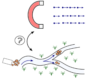
Given these premises, this work analyses how the transition from a balanced towards an unbalanced bifurcation can be conceived as a morphodynamic second-order phase transition analogue to thermodynamic ferromagnetism. The definition of a bifurcation parameter inversely proportional to the width-to-depth ratio replaces the temperature as critical parameter. The analogy is unravelled through a fully analytical treatment of a consolidated modelling framework, which is framed into a classical theory of critical phenomena.
2. The theoretical bifurcation model
The starting point is the two-cell scheme proposed by Bolla Pittaluga, Repetto & Tubino (Reference Bolla Pittaluga, Repetto and Tubino2003) (hereafter denoted BRT). This model has proved to reproduce successfully the basic physical processes acting in bifurcation dynamics (e.g. Burge Reference Burge2006; Zolezzi, Bertoldi & Tubino Reference Zolezzi, Bertoldi and Tubino2006; Bertoldi & Tubino Reference Bertoldi and Tubino2007; Salter, Voller & Paola Reference Salter, Voller and Paola2019). The BRT model retains in a quasi-two-dimensional fashion the feature essential for the occurrence of bifurcation instability, namely the development of a transverse bed gradient just upstream of the bifurcation under suitable flow conditions. An upstream channel is assumed to split into two smaller and geometrically symmetric downstream channels ( $l$ and
 $r$; figure 3). The channel banks are fixed, so the planform geometry does not change in time. In proximity of the bifurcation, two cells
 $W_{0}^{*}\xi$ long allow for the lateral exchange of flow and sediment at the node, where
 $W_{0}^{*}$ is the main channel width, and
 $\xi$ is an order one coefficient. The node is fed by a constant and uniformly distributed water and sediment supply, while at the downstream end, the branches are characterized by a constant and equal water level. It follows that in such a configuration, in the absence of any external forcing factor, there is no preferential path for water and sediment to be distributed downstream.
Geometrical sketch of the free bifurcation BRT model with notation. Plan view and cross-sectional view.

The nodal cells are allowed to evolve in time by assuming that flow field adapts instantaneously to bed variations at the bifurcation. Let  $q^{*}$ and
 $q_{s}^*$ be the flow and sediment flux per unit width, and let
 $\eta ^{*}$ be the bed elevation. The mass conservation equations for the two cells can be written in the form
 $$\begin{gather} (1-\lambda_{p})\,\frac{{\rm d} \eta_{l}^{*}}{{\rm d}t^{*}} =- \frac{q_{sl}^{*}-q_{s0}^{*}}{\xi W_{0}^{*}} + \frac{1}{2}\,\frac{q_{sy}^{*}}{W_{0}^{*}}, \end{gather}$$
 $$\begin{gather}(1-\lambda_{p})\,\frac{{\rm d} \eta_{r}^{*}}{{\rm d}t^{*}} =- \frac{q_{sr}^{*}-q_{s0}^{*}}{\xi W_{0}^{*}} - \frac{1}{2}\,\frac{q_{sy}^{*}}{W_{0}^{*}}, \end{gather}$$
with  $q_{sy}^{*}$ the transversal sediment flux, and
 $\lambda _{p}$ the bed porosity.
In order to compute the lateral flow and sediment distribution at the bifurcation, BRT employed a well-known approach of two-dimensional morphodynamics problems. Sediments moving as bedload tend to feel the action of gravity, and in turn are deflected with respect to the streamwise direction. A simple generalization for this mechanism can be written as (e.g. Parker Reference Parker1984)
 \begin{equation} q_{sy}^{*} = q_{s0}^{*}\left[ \frac{1}{2 \xi} \left( \frac{q_{l}^{*} - q_{0}^{*}}{q_{0}^{*}} \right) - \frac{2r}{\sqrt{\tau_{*0}}}\,\frac{\eta_{l}^{*}-\eta_{r}^{*}}{W_{0}^{*}} \right] , \end{equation}
where  $r$ is a dimensionless parameter controlling the magnitude of the gravitation-induced sediment flux deflection with respect to water flow direction (e.g. Ikeda Reference Ikeda1982), and
 $\tau _{*0}$ is the Shields mobility number. The latter parameter is given by
 $\tau _{*0} = D_{0}^{*} S_{0}/[(s_{g}-1) d_{s}^{*}]$, with
 $s_{g}$ the ratio between sediment and water density,
 $d_{s}^{*}$ a reference grain size relative to a uniform bottom sediment composition,
 $D_{0}^{*}$ the main channel flow depth, and
 $S_{0}$ the main channel slope. Note that (2.2) neglects implicitly the possible deviation due to bed roughness that grains experience as they are transported. It has been shown that this effect gives rise to a diffusive component in the lateral transport, hindering the gravitational term (Seizilles et al. Reference Seizilles, Lajeunesse, Devauchelle and Bak2014; Abramian, Devauchelle & Lajeunesse Reference Abramian, Devauchelle and Lajeunesse2019). However, it can be proved that in the present problem, the diffusive contribution is approximately two orders of magnitude smaller than the slope-induced effect, thus it can be disregarded safely.
The formulation is completed by requiring the continuity of water mass  $q_{0}^{*}=(q_{l}^{*} + q_{r}^{*} )/2$, and the condition of negligible cross-sectional deformation of the free surface
 $H_{0}^{*}=H_{l}^{*}=H_{r}^{*}$ at the node. Flow and sediment transport in the downstream channels are expressed by assuming that a steady uniform flow takes place. A classical Chézy formula for a rectangular wide channel is employed, which allows us to write the water discharge as
 $q^{*} = c D^{*3/2} \sqrt {S g}$, with
 $c=f(D^{*})$ the Chézy coefficient, and
 $g$ the gravity acceleration. The sediment transport is estimated as
 $q^{*}_{s} = \sqrt {g (s_{g}-1) d_{s}^{*3}}\,\varPhi (\tau _{*},D^{*})$, with
 $\varPhi$ an equilibrium transport function for which different expressions are available in the literature.
It is convenient to write the governing equations in dimensionless form. The following set of dimensionless quantities is introduced:
 \begin{equation} W := \frac{W^{*}}{W^{*}_{0}}, \quad q := \frac{q^{*}}{q^{*}_{0}}, \quad q_{s} := \frac{q^{*}_{s}}{q^{*}_{s0}}, \quad (\eta, D) := \frac{(\eta^{*}, D^{*})}{D_{0}^{*}} , \end{equation}
which allows us to cast the sediment mass balance (2.1) as
 $$\begin{gather} \frac{{\rm d}}{{\rm d}t}(D_{l}-H_{l}) = q_{sl} - 1 - 2 \xi q_{sy}, \end{gather}$$
 $$\begin{gather}\frac{{\rm d}}{{\rm d}t}(D_{r}-H_{r}) = q_{sr} - 1 + 2 \xi q_{sy}, \end{gather}$$
with
 \begin{equation} 2 \xi q_{sy}= q_{l} - 1 - \frac{2 \xi r}{\mathcal{B}_{0} \sqrt{\tau_{*0}}}\,(D_{r}-D_{l}) . \end{equation}
The parameter  $\mathcal {B}_{0}:=W_{0}^{*}/(2 D_{0}^{*})$ is the half width-to-depth ratio of the main channel. Time
 $t^{*}$ is scaled by means of the bifurcation time scale
 $T_{bif}^{*}$, which arises naturally from dimensional considerations:
 \begin{equation} T_{bif}^{*} = \frac{(1-\lambda_{p})\xi D_{0}^{*} W_{0}^{*}}{q_{s0}^{*}} . \end{equation}
The nonlinear differential equations for sediment mass balance (2.4), once (2.5) is included properly and enforcing flow continuity, can be expressed opportunely in terms of their sum and difference:
 $$\begin{gather} \frac{{\rm d} \Delta D}{{\rm d}t} = 2 \left[ \Delta q_s - \Delta q - 2 \mathcal{R}\,\Delta D \right], \end{gather}$$
 $$\begin{gather}\frac{{\rm d}\bar{D}}{{\rm d}t} = \overline{q_s} - \bar{q}, \end{gather}$$
where  $\mathcal {R}$ is the bifurcation parameter (Ragno et al. Reference Ragno, Redolfi and Tubino2021)
 \begin{equation} \mathcal{R} := \frac{\xi r}{\mathcal{B}_{0} \sqrt{\tau_{*0}}} , \end{equation}
which incorporates the empirical parameters  $r$ and
 $\xi$. Physically, the bifurcation parameter defines the magnitude and extent of the gravitational pull on sediment flux deflection, thus providing a first-order control on the stability of the bifurcation. For actual rivers, typically the bifurcation parameter ranges between
 $10^{-1}$ and
 $10^{0}$ (Ragno et al. Reference Ragno, Redolfi and Tubino2021).
The first equation of system (2.7) describes the evolution in terms of asymmetry variables, namely quantities that take non-zero values just in the unbalanced state:
 \begin{equation} \Delta D := D_{l} - D_{r} , \quad (\Delta q,\Delta q_{s}) := \tfrac{1}{2} \left(q_{l}-q_{r}, q_{sl}-q_{sr} \right) , \end{equation}
with  $(\Delta q,\Delta q_{s})$ functions of
 $\Delta D$ and of the reference hydraulic and transport conditions. Conversely, equation (2.7b) is simply a function of mean variables, thus not depending on the degree of displacement of the system:
 \begin{equation} \bar{D} := \tfrac{1}{2}(D_{l} + D_{r}) , \quad (\bar{q} ,\overline{q_s} ) := \tfrac{1}{2} \left(q_{l}+q_{r}, q_{sl}+q_{sr} \right). \end{equation}
3. A Landau's analogy
3.1. The free response
An examination of the differential problem (2.7) suggests that  $\mathcal {R}$ fundamentally controls the dynamics of the system. As emphasized by previous theoretical studies (Ragno et al. Reference Ragno, Redolfi and Tubino2021; Ragno, Tambroni & Bolla Pittaluga Reference Ragno, Tambroni and Bolla Pittaluga2022b), the bifurcation parameter, which is inversely proportional to
 $\mathcal {B}_{0}$, is found to control the number and relative stability of equilibria: if
 $\mathcal {R}$ is higher than the critical threshold
 $\mathcal {R}_{cr}$, then flow and sediment fluxes are distributed equally at the bifurcation. In this case,
 $\Delta D =0$. The situation changes radically when
 $\mathcal {R}$ is lower than
 $\mathcal {R}_{cr}$, since the balanced solution becomes unstable, with the system attaining a stable state where one of the two branches captures most of the discharge, i.e.
 $\Delta D \ne 0$. According to the BRT model, the critical bifurcation parameter is given by
 \begin{equation} \mathcal{R}_{cr} = \tfrac{1}{4} \left(\varPhi_{T} + \varPhi_{D} - c_{D} - \tfrac{3}{2} \right) , \end{equation}
where coefficients  $\varPhi _{T}$,
 $\varPhi _{D}$ and
 $c_{D}$, which measure the sensitivity of the sediment transport rate and Chézy coefficient to variations of flow depth and Shields parameter, are defined as
 \begin{equation} \varPhi_{T}:=\left.\frac{\tau_{*0}}{\varPhi_{0}}\,\frac{\partial \varPhi}{\partial \tau_{*}}\right|_{\tau_{*0}}, \quad \varPhi_{D}:=\left.\frac{D_{0}}{\varPhi_{0}}\,\frac{\partial \varPhi}{\partial D}\right|_{D_{0}}, \quad c_{D}:=\left.\frac{D_{0}}{c_{0}}\,\frac{\partial c}{\partial D}\right|_{D_{0}} , \end{equation}
and their explicit expression depends on the friction and transport formula adopted (Redolfi, Zolezzi & Tubino Reference Redolfi, Zolezzi and Tubino2019).
Taking the viewpoint of condensed matter physics, here it is proposed that the critical bifurcation parameter can be conceived as a morphodynamic analogue of the Curie temperature above which spontaneous magnetization disappears in a ferromagnetic material (e.g. Kadanoff et al. Reference Kadanoff, Gotze, Hamblen, Hecht, Lewis, Palciauskas, Rayl and Swift1967; Wilson Reference Wilson1983). If this analogy is pursued, then it seems reasonable to follow the fundamental idea apparently first introduced by Landau (Reference Landau1937), who suggested to study the behaviour of systems showing a second-order phase transition near a critical point in terms of an order parameter (e.g. Landau & Lifshitz Reference Landau and Lifshitz1980; Domb Reference Domb1996). In this problem, the order parameter arises naturally from system (2.7), coinciding with the depth elevation asymmetry,  $\Delta D$.
In order to measure the deviation from the critical point, the parameter  $\epsilon$ is introduced:
 \begin{equation} \epsilon := \frac{\mathcal{R}_{cr}-\mathcal{R}}{\mathcal{R}_{cr}} \ll 1. \end{equation}
From this, several properties of the order parameter follow (Kadanoff et al. Reference Kadanoff, Gotze, Hamblen, Hecht, Lewis, Palciauskas, Rayl and Swift1967). First,  $\Delta D = 0$ when
 $\epsilon < 0$ (subcritical phase), but
 $\Delta D$ is different from zero when
 $\epsilon >0$. Second, a discontinuous jump of
 $\Delta D$ is absent when
 $\mathcal {R} \rightarrow \mathcal {R}_{cr}$. Third, when
 $\epsilon > 0$ (supercritical phase),
 $\Delta D$ can assume two or more values under the same physical conditions. Indeed, either the left or the right branch can capture the largest fraction of water and sediment.
The phase transition, i.e. the evolution of a river bifurcation from a balanced to an unbalanced flux partitioning, can be solved once the functional relation  $f(\epsilon,\Delta D)$ is computed. Near criticality, where the order parameter
 $\Delta D$ is small, each variable, say generically
 $X$, is assumed to be a slowly varying function in time and analytic in
 $\epsilon$. Thus the slow time scale
 $T=\epsilon t$ is defined, and the following expansion of the solution holds:
 \begin{equation} X = X_{0} + \sum_{j=1}^{3} X_{j} (\epsilon^{\beta})^{j} + O(\epsilon^{4\beta}), \end{equation}
where the value of the expansion coefficient  $\beta$ is a priori unknown.
A strategy to determine the order of the critical parameter  $\epsilon$ is to follow a heuristic argument adopted widely in the field of hydrodynamic and morphodynamic stability (e.g. Stuart Reference Stuart1960; Colombini, Seminara & Tubino Reference Colombini, Seminara and Tubino1987): reason of symmetry suggests that the linear component
 $X_{1}$ is modified at the third order, where the term
 $\epsilon \,{\rm d}(\epsilon ^{\beta } X )/{\rm d}T$ must be balanced by linear and nonlinear terms proportional to
 $\epsilon ^{3\beta }$. Consequently, the critical index
 $\beta$ is equal to
 $1/2$, which corroborates the analogy with Landau's theory, as discussed below.
Substituting (3.4) into system (2.7), and equating like powers of  $\epsilon$, a cascade of algebraic problems is obtained. At the order
 $\epsilon ^{3/2}$, the following nonlinear ordinary differential equation governing the evolution of the order parameter
 $\Delta D$ is found:
 \begin{equation} \frac{{\rm d} \Delta D}{{\rm d}T} = \epsilon \alpha_{1}\,\Delta D + \alpha_{2}(\Delta D^{3}), \end{equation}
where the coefficients  $\alpha _{1}$ and
 $\alpha _{2}$ depend on
 $\epsilon$, and on the specific reference conditions (i.e.
 $\tau _{*0}$ and
 $c_{0}$). Their expression is reported in Appendix A along with the computations to derive (3.5).
Equation (3.5) is of the Stuart–Landau type, and admits an analytical solution of the form
 \begin{equation} \Delta D(t)= \left[ - \frac{\alpha_{2}}{\alpha_{1}} + \left(\Delta D(0)^{-2} + \frac{\alpha_{2}}{\alpha_{1}} \right) \exp(- \epsilon \alpha_{1} t) \right]^{-1/2} . \end{equation}
If the cubic term in (3.5) is neglected, then the order parameter  $\Delta D$ exhibits an exponential behaviour, with the growth rate governed by the coefficient
 $\alpha _{1}$. For
 $\epsilon >0$, the nonlinear term inhibits the unbounded growth since the algebraic coefficients
 $\alpha _{1}$ and
 $\alpha _{2}$ have opposite sign (figure 9). Hence in the first stages, the growth of asymmetry development is governed by the linear component of the solution. In this phase, the solution follows a nearly exponential behaviour that is proportional to
 $\exp (\alpha _{1} t)$. Then higher-order terms become important, and the curve changes concavity until it reaches the final equilibrium state (figure 4).
Evolution of the order parameter  $\Delta D$ as scaled by its equilibrium value
 $\Delta D_{eq}$ in a reference supercritical phase. The dashed line denotes the linear solution. Without loss of generality, the plot refers to a gravel-bed river for which the Parker (Reference Parker1978) transport formula is used.

Thus as  $t \rightarrow \infty$, an equilibrium solution
 $\Delta D_{eq}$ is reached asymptotically:
 \begin{equation} \Delta D_{eq} ={\pm} \sqrt{- \frac{\alpha_{1}}{\alpha_{2}}}\,\epsilon^{1/2} . \end{equation}
The equilibrium solution (3.7) describes mathematically a supercritical pitchfork bifurcation (figure 5a). When  $\epsilon <0$, the only real solution is
 $\Delta D_{eq} = 0$, i.e. the balanced bifurcation. Conversely, two real solutions exist when
 $\epsilon >0$, showing physically the steady state where one of the two branches captures most of the water and sediment fed at the bifurcation.
(a) Phase diagram of a free bifurcation. The order parameter is plotted as a function of  $\epsilon$. The yellow star indicates the critical point. (b) Potential function
 $\mathcal {G}$ against the steady order parameter
 $\Delta D_{eq}$ for two values of the scaled bifurcation parameter
 $\epsilon$. Without loss of generality, both plots refer to a gravel-bed river for which the Parker (Reference Parker1978) transport formula is adopted.

From (3.7), it follows that in the supercritical phase, the order parameter is proportional to the scaled bifurcation parameter  $\epsilon ^{\beta }$, with
 $\beta = 1/2$. Despite the ratio between
 $\alpha _{1}$ and
 $\alpha _{2}$ in general not being constant, the critical exponent keeps the same value. This observation highlights an essential property of the system, namely universality. Such universal behaviour is a typical feature of phase transitions (e.g. Kadanoff Reference Kadanoff1990). The critical exponent conforms with the value obtained from the mean-field theory employed by Landau (Reference Landau1937). In order to obtain the latter result, Landau followed a classic rule of thermodynamics whereby the most probable value of any (macroscopic) thermodynamic variable is the one that minimizes the free energy. Following the thread of Landau, a morphodynamic potential
 $\mathcal {G}=f(\epsilon,\Delta D; \tau _{*0},c_{0})$ can be defined as
 \begin{equation} \mathcal{G} =- \left[ \tfrac{1}{2}\epsilon\alpha_{1}\,\Delta D^{2} + \tfrac{1}{4}\alpha_{2}\,\Delta D^{4} \right], \end{equation}
where no odd powers of  $\Delta D$ are present due to the symmetry requirement. In other words, the morphodynamic potential cannot depend on the sign of
 $\Delta D$ if no external factors are included.
Figure 5(b) shows the morphodynamic potential of a reference gravel-bed river for which a typical threshold transport function is employed. Overall, the residual effect of Chézy coefficient  $c_{0}$ on
 $\alpha _{1}$ and
 $\alpha _{2}$ is very weak, to the point that it vanishes exactly when adopting a friction formula of the Manning–Strickler type (e.g. Ferguson Reference Ferguson2007; Parker et al. Reference Parker, Wilcock, Paola, Dietrich and Pitlick2007). Similarly, there is no residual effect of the Shields number
 $\tau _{*0}$ when considering sand-bed cases, where the transport function is usually estimated through a power-law relation, while a rather important effect remains in gravel-bed cases. Consequently, for sand-bed rivers, the equilibrium value predicted by the model can be approximated by the expression
 \begin{equation} \Delta D_{eq}^{sand} ={\pm} 0.55 \epsilon^{1/2}, \end{equation}
which, it is worth stressing, is strictly valid for  $\epsilon \rightarrow 0$.
Summarizing, in this subsection it has been shown how river bifurcations can be interpreted as critical phenomena showing several analogies with thermodynamic phase transitions. The definition of the potential (3.8) is particularly useful, since it allows us to elucidate characteristics of the morphodynamic system taking advantage of theories developed in the context of condensed matter physics. Specifically, it will be seen below how the morphodynamic potential proves to be convenient to investigate the response of bifurcations to an (applied) external forcing.
3.2. The effect of an external forcing
Up to this point, the free response of the system has been analysed. However, in nature, bifurcations are seldom free, with allogenic forcing factors coexisting with the free response. Physically, a forcing effect can be caused by a slope advantage to one of the two branches (e.g. due to backwater effects, different channel lengths due to meander cut-offs) or by the curvature of the main channel causing a secondary flow component at the node (Redolfi et al. Reference Redolfi, Zolezzi and Tubino2019). In the context of Landau theory, an external yet physically unspecified steady forcing  $\mathcal {F}$ is considered here. This is equivalent to considering
 $\mathcal {F}$ acting on a much slower time scale than the intrinsic time scale of bifurcation evolution (2.6). If this forcing is assumed to be linearly dependent in the order parameter, then the (free) potential (3.8) is modified accordingly as
 \begin{equation} \mathcal{G} =- \left[\tfrac{1}{2} \epsilon \alpha_{1}\,\Delta D^{2} + \tfrac{1}{4} \alpha_{2}\,\Delta D^{4} - \varphi \mathcal{F}\,\Delta D \right], \end{equation}
which, when minimized, yields
 \begin{equation} \mathcal{F} = \varphi^{-1} ( \epsilon \alpha_{1}\,\Delta D_{eq} + \alpha_{2}\,\Delta D_{eq}^{3}) , \end{equation}
where  $\varphi$ is a calibration coefficient.
One direct consequence of the applied forcing is the non-zero value of  $\Delta D_{eq}$ for any given value of
 $\epsilon$. In other words, there is no spontaneous symmetry breaking of the system (figure 6a). In the subcritical phase, the system is dominated by the forcing effect, with the depth asymmetry varying smoothly with
 $\mathcal {F}$. In this case, there is just one real stable solution. The picture changes radically in the supercritical phase. As (3.11) indicates, there is a range of values of
 $\mathcal {F}$ such that three real solutions exist. However, one of these solutions turns out to be unstable.
The relationship between the free and forced responses. (a) Order parameter as a function of forcing  $\mathcal {F}$. (b) Forcing threshold
 $\mathcal {F}_{t}$ against
 $\epsilon$. Coloured lines stand for gravel-bed rivers with different values of Shields number
 $\tau _{*0}$. The dashed line denotes a reference sand-bed river.

The range of values of  $\mathcal {F}$ where the solution is no longer single-valued, thus
 $-\mathcal {F}_{t} < \mathcal {F}< \mathcal {F}_{t}$, can be derived readily by differentiating (3.11) with respect to
 $\Delta D_{eq}$. The quantity
 $\mathcal {F}_{t}$ is given by
 \begin{equation} \mathcal{F}_{t} \sim \left(\alpha_{1}|\epsilon| \right)^{3/2} \alpha_{2}^{-1/2}, \end{equation}
and it provides the threshold value of the forcing whereby the free and forced responses have the same order of magnitude (Landau & Lifshitz Reference Landau and Lifshitz1980). The threshold  $\mathcal {F}_{t}$ corresponds to a forcing able to suppress entirely the spontaneous response of the system. According to (3.12), higher values of the threshold are required as long as the deviation of the system from critical conditions increases. The characteristic value of the spontaneous response is provided by (3.7), namely
 $\Delta D_{eq}^{S} \sim (\alpha _{1}|\epsilon |/\alpha _{2})^{1/2}$, while the forced-induced component of the order parameter is estimated as
 $\Delta D_{eq}^{F} \sim \chi \mathcal {F}$. The quantity
 $\chi$ is an equivalent of the magnetic susceptibility, namely a measure of the sensitivity of the order parameter under the action of an external forcing. The morphodynamic susceptibility is described by
 $\chi \sim (\alpha _{1} \epsilon )^{-1}$, indicating that the system can be highly affected by weak variations of the forcing as long as
 $\epsilon$ approaches criticality.
The computation of function  $\mathcal {F}_{t}$ enables the definition of a morphodynamic bound that divides two qualitatively different behaviours of the bifurcation system when subjected to allogenic factors (figure 6b). When
 $\mathcal {F} \gg \mathcal {F}_{t}$, the system is forced-dominated, with the free response almost completely suppressed. In this case, the order parameter can be estimated from (3.11), and it is equal to
 $\Delta D_{eq}^{F} \sim (\mathcal {F}/\alpha _{2})^{1/3}$. On the other hand, when
 $\mathcal {F} < \mathcal {F}_{t}$, an interaction between the autogenic and allogenic dynamics is promoted, with the possibility of undergoing hysteresis and counterintuitive solutions of the bifurcation system.
Nevertheless, the definition of the forcing might appear abstract to the reader. To overcome this limitation, the recent numerical analysis performed by Redolfi et al. (Reference Redolfi, Zolezzi and Tubino2019), in which different kind of forcing effects are modelled physically, lends itself to being particularly instructive. Assume that the upstream channel is a meander bend. Redolfi et al. (Reference Redolfi, Zolezzi and Tubino2019) have shown that channel curvature, here denoted  $\mathcal {C}$, generates a further spiral flow component in the equation of transverse transport (2.2), which produces an uneven distribution of the incoming fluxes at the node. In the present modelling framework, this additional term is absent, since the forcing
 $\mathcal {C}$ is imposed simply as linearly dependent on the order parameter. However, as shown in figure 7, the analytical solution (3.12) provides a reasonable estimate of the forcing threshold when compared with the numerical solution. It is worth mentioning that in order to make the analytical results consistent with Redolfi et al. (Reference Redolfi, Zolezzi and Tubino2019), a slightly different definition of the critical parameter is adopted. Namely, the deviation from criticality
 $\hat {\epsilon }$ is defined with respect to the half width-to-depth ratio:
 \begin{equation} \hat{\epsilon} = \frac{\mathcal{B} - \mathcal{B}_{R}}{\mathcal{B}} , \end{equation}
where  $\mathcal {B}_{R}$ is the resonant half width-to-depth ratio, which defines the threshold between prevailing downstream or upstream influence of two-dimensional morphodynamic changes (Zolezzi & Seminara Reference Zolezzi and Seminara2001; Redolfi et al. Reference Redolfi, Zolezzi and Tubino2016). Recalling the physical meaning of morphodynamic resonance, when the channel width-to-depth ratio is smaller (greater) than the resonant value, a regular sequence of damped steady alternate bars is predicted to form downstream (upstream) of a persistent obstacle (Zolezzi & Seminara Reference Zolezzi and Seminara2001). If, as in the present work, the obstacle is a channel bifurcation, then super-resonant conditions correspond to the case of an unbalanced bifurcation, with the resonant width-to-depth ratio related closely to the critical bifurcation parameter discussed previously. Specifically, as suggested by Redolfi et al. (Reference Redolfi, Zolezzi and Tubino2019), the resonant value can be computed by calibrating the bifurcation length
 $\xi$ to obtain the same critical width-to-depth ratio. It can be realized that the alternative critical parameter (3.13) does not change the qualitative result.
Comparison between the analytical expression (3.12) of the forcing threshold, which is given for different values of coefficient  $\varphi$ (blue lines), and the numerical solution of Redolfi et al. (Reference Redolfi, Zolezzi and Tubino2019) (black line). The forcing is exemplified by the channel curvature
 $\mathcal {C}$, while
 $\hat {\epsilon }$ is the scaled half width-to-depth ratio (3.13).

4. Comparison with data
In order to check the consistency and correctness of theory, a comparison with available data is carried out. This is shown in figure 8, where equilibrium conditions are expressed in terms of a discharge asymmetry index  $\Delta Q_{eq}=(Q_{l}^{*}-Q_{r}^{*})/Q_{0}^{*}$. The closed form of
 $\Delta Q_{eq}$ can be found readily from (3.7), yielding:
 \begin{equation} \Delta Q_{eq} = \tfrac{1}{2} \left(c_{D} +\tfrac{3}{2} \right) \Delta D_{eq}\,\epsilon^{1/2} . \end{equation}
Comparison between estimated and measured values of the water discharge asymmetry  $\Delta Q_{eq}$ with available data. (a) Laboratory experiments of Bertoldi & Tubino (Reference Bertoldi and Tubino2007) relative to a gravel-bed river, where the markers denote different longitudinal bed slopes
 $S$ of the laboratory data. The Parker (Reference Parker1978) formula is adopted for the computation of the transport function. (b) Numerical runs (ES08, from Edmonds & Slingerland Reference Edmonds and Slingerland2008) and field measurements of bifurcations in the Columbia River and Cumberland Marshes (Col and Cumb, from Bolla Pittaluga et al. Reference Bolla Pittaluga, Coco and Kleinhans2015) relative to sand-bed rivers. The root-mean-square error of the analytical result is (a) 0.28, and (b) 0.21.

Data cover the 25 laboratory flume experiments performed by Bertoldi & Tubino (Reference Bertoldi and Tubino2007), the 11 numerical runs of Edmonds & Slingerland (Reference Edmonds and Slingerland2008), and 11 bifurcations in natural sand-bed rivers reported by Bolla Pittaluga, Coco & Kleinhans (Reference Bolla Pittaluga, Coco and Kleinhans2015). Both experiments and numerical runs refer to free bifurcations.
As shown in the plot, the theoretical predictions are roughly in agreement with the measured  $\Delta Q_{eq}$ values as long as the discharge asymmetry is approximately below
 $0.5$. The discrepancies appearing for larger values of
 $\Delta Q_{eq}$ are in accordance with the range of validity of theory. Indeed, the magnitude of
 $\Delta Q_{eq}$ is a proxy of the relative deviation from critical conditions
 $\epsilon$. Another source of inaccuracy is that a given value of the empirical parameters
 $r$ and
 $\xi$, here taken equal to
 $0.5$ and
 $4$, respectively, must be prescribed. However, it will be discussed in the next section how the dimensionless length is in general not a constant, but depends on
 $\epsilon$. Finally, it is worth highlighting that natural rivers are not necessarily at equilibrium, and are probably affected by the presence of one or more external forcings.
5. Discussion and conclusion
The foregoing theoretical analysis re-examines the widely used BRT bifurcation model in the framework of classical Landau theory of second-order phase transitions. The classical approach employed reflects the purely macroscopic character of the governing variables adopted in the formulation. Thus the model is classically morphodynamic in its nature, with the most probable value of the order parameter being simply the mean value (Kadanoff et al. Reference Kadanoff, Gotze, Hamblen, Hecht, Lewis, Palciauskas, Rayl and Swift1967). This implies that all the possible microscopic fluctuations in the order parameter are ruled out. It is arguable that autogenic fluctuations would be related closely to the motion and interactions among sediment grains. Taking into account autogenic fluctuations would require a radical change of perspective based in statistical mechanics. This change of perspective is likely to affect the quantitative estimation of critical exponents. The critical exponents are the same for all phase transitions studied accordingly with the Landau theory, prefiguring a universality of critical phenomena as mentioned before. That is, actual bifurcations are expected to share the same behaviour close to criticality, which is independent of the detailed characteristics of single rivers (e.g. climate, sediment composition, dominant transport modality). It is interesting to note that this kind of universality has been observed recently by Ragno, Redolfi & Tubino (Reference Ragno, Redolfi and Tubino2022a) for the spatial scaling of bifurcation–confluence systems.
Yet it has long been known that the set of critical indices predicted by Landau theory turns out to differ quantitatively with respect to laboratory experiments. For example, according to Landau, the correlation length – which can be thought as the distance at which the magnetic moment alignment of single electrons induces a preferential alignment for the others (Wilson Reference Wilson1983) – is predicted to behave near the transition point following  $\epsilon ^{-\nu }$, with
 $\nu =1/2$. Quantitatively, experiments showed that
 $\nu \simeq 0.6$ (e.g. Kadanoff et al. Reference Kadanoff, Gotze, Hamblen, Hecht, Lewis, Palciauskas, Rayl and Swift1967; Wilson & Kogut Reference Wilson and Kogut1974). The analogue of correlation length for the present problem is the coefficient
 $\xi$, which represents the dimensionless length controlling the upstream morphodynamic influence. Here,
 $\xi$ is assumed as a constant that is embedded in the definition of parameter
 $\mathcal {R}$. Previous experimental and theoretical investigations indicated that
 $\xi$ depends substantially on
 $\epsilon$ (Bertoldi & Tubino Reference Bertoldi and Tubino2007; Redolfi et al. Reference Redolfi, Zolezzi and Tubino2016). In particular, Redolfi et al. (Reference Redolfi, Zolezzi and Tubino2016) demonstrated that
 $\xi$ follows a decreasing trend for larger deviation from critical conditions. The relationship between
 $\xi$ and
 $\epsilon$ turned out to be nearly inversely proportional to the damping rate of the steady alternate bar pattern triggered by the bifurcation, thus suggesting
 $\nu \simeq 1$. The damping rate vanishes at resonant conditions, which implies that
 $\xi$ tends to diverge approaching the critical point.
A second important feature of the analysis concerns the use of a general mathematical formulation to provide a sound interpretation of the state-of-the-art BRT bifurcation model. Despite its limitations, the approach pursued by Landau has its main merit in providing a solid framework able to give a qualitatively correct representation of what happens close to criticality (see the discussion in Kadanoff Reference Kadanoff2009). The equilibrium configurations of the system are nothing but minima of the potential function  $\mathcal {G}$ (see (3.8)). Moreover, the theoretical model lends itself to be extended, with a relatively modest effort, for investigating the effect of forcing factors. The analysis recognizes how the morphodynamic response depends on the distance from critical conditions even when a forcing is present. The forcing threshold, for which the proportionality
 $\mathcal {F}_{t} \propto \epsilon ^{3/2}$ holds, identifies the order of magnitude of a forcing effect such that an interaction between the allogenic and autogenic response of the system occurs (figure 6). Note that the relationship between free and forced mechanisms is at the core of other morphodynamic processes such as bar–bend interaction in meandering streams (Seminara & Tubino Reference Seminara and Tubino1989; Tubino & Seminara Reference Tubino and Seminara1990).
To conclude, it is argued here that the apparent analogy between morphodynamic and thermodynamic phase transitions, which is exemplified here by channel bifurcations, could be a more general characteristic of other sedimentary patterns. In particular, it has been mentioned how the dynamics of channel bifurcations is related closely to bars, which have been recognized as a fundamental morphological feature for pattern formation (e.g. Seminara Reference Seminara2010; Church & Ferguson Reference Church and Ferguson2015). A potential unified treatment of morphodynamic critical phenomena deserves a justification in morphological terms, and needs to be verified through systematic laboratory and field investigations. On the other hand, potentially, a mathematical reformulation of geomorphological problems based on the theory of phase transitions from the viewpoint of condensed matter physics could allow us to improve our understanding of the apparent similar nature of sedimentary patterns, which often seem to be not dependent on the specific underlying properties of single rivers. Moreover, it is emphasized that this change of perspective would allow us to take advantage of theories and mathematical tools, such as the renormalization group (e.g. Wilson Reference Wilson1971; Wilson & Kogut Reference Wilson and Kogut1974), that lead physicists to an explanation of the observed universality characterizing phase transitions.
Acknowledgements
The author deeply thanks M. Tubino and M. Redolfi for fruitful discussions and constant support. Also, the fair criticism raised by two anonymous referees has significantly improved the paper.
Funding
This work has been supported by the Italian Ministry of Education, University and Research (MIUR) in the frame of the ‘Departments of Excellence’ grant L. 232/2016, and by ‘Agenzia Provinciale per le Risorse Idriche e l'Energia’ (APRIE) – Provincia Autonoma di Trento.
Declaration of interests
The author reports no conflict of interest.
Data availability statement
All data are from published literature.
Appendix A. Derivation of coefficients  $\alpha _{1}$ and $\alpha _{2}$


In this appendix, the derivation of the Stuart–Landau equation (3.5) is provided.
As mentioned in the main text, by substituting the expansion (3.4) into the differential system (2.7a) and (2.7b), introducing the slow time scale  $T=\epsilon t$, and equating like powers of
 $\epsilon$, a cascade of algebraic problems is obtained.
At first order, the following algebraic system is found:
 $$\begin{gather} \bar{D}_{1} = 0 , \end{gather}$$
 $$\begin{gather}\Delta D\,(t_{1} - s_{1} - 4 \mathcal{R}_{cr}) = 0 , \end{gather}$$
with  $t_{1}=\varPhi _{T} + \varPhi _{D}$ and
 $s_{1}=3/2 + c_{D}$.
Equation (A1a) states simply that the linear solution is fully antisymmetric, as is to be expected. It follows that  $S_{1}/S_{0} = 0$, which means that linearly, the channel slope of the bifurcates is equal to the reference slope of the main channel. Equation (A1b) allows us to determine marginal conditions, namely the critical value of the bifurcation parameter
 $\mathcal {R}_{cr}$:
 \begin{equation} \mathcal{R}_{cr} = \tfrac{1}{4} (t_{1} - s_{1}) . \end{equation}
At the next order, there is a correction of channel slope  $S_{2}/S_{0}$ that is different from zero. This contribution can be derived readily from the flow mass conservation, yielding
 \begin{equation} \frac{S_{2}}{S_{0}} =- \left[2 s_{1} \bar{D}_{2} + 2 s_{2}\,\Delta D^{2} \right] , \end{equation}
with
 \begin{equation} s_{2}= \frac{1}{8}\left( c_{DD} + 3c_{D} + \frac{3}{4} \right), \quad c_{DD}:=\left.\frac{1}{c_{0}}\, \frac{\partial^{2} c}{\partial D^{2}}\right|_{D_0} . \end{equation}
Since variables inside the square brackets of (A3) are positive quantities, it follows that  $S_{2}/S_{0}$ is negative, thus indicating a gentler slope of the bifurcates with respect to the main channel for larger deviation from criticality (i.e. higher amount of displacement).
The correction at second order for the mean water depth  $\bar {D}_{2}$ reads as
 \begin{equation} \bar{D}_{2} = l_{1}\,\Delta D^{2}, \end{equation}
with
 \begin{equation} l_{1} = \frac{2\varPhi_{T}s_{2} - t_{2}}{t_{1} -2 \varPhi_{T}s_{1}}, \quad t_{2}=\frac{1}{8}\left( \varPhi_{TT} + \varPhi_{DD} + 2 \varPhi_{TD} \right) . \end{equation}
The coefficients  $\varPhi _{TT}$,
 $\varPhi _{DD}$ and
 $\varPhi _{TD}$ are defined as
 \begin{equation} \varPhi_{TT}:=\left.\frac{\tau_{*0}^{2}}{\varPhi_{0}}\,\frac{\partial^{2} \varPhi}{\partial \tau_{*}^{2}}\right|_{0}, \quad \varPhi_{DD}:=\left.\frac{1}{\varPhi_{0}}\,\frac{\partial^{2} \varPhi}{\partial D^{2}}\right|_{0}, \quad \varPhi_{TD}:=\left.\frac{\tau_{*0}}{\varPhi_{0}}\, \frac{\partial^{2} \varPhi}{\partial \tau_{*} \partial D}\right|_{0} . \end{equation}
It follows that  $S_{2}/S_{0}$ is given by
 \begin{equation} \frac{S_{2}}{S_{0}} = l_{2}\,\Delta D^{2}, \end{equation}
with
 \begin{equation} l_{2} =- 2(s_{1}l_{1} + s_{2}) . \end{equation}
Finally, at cubic order, some tedious algebra is needed to determine the correction of flow and sediment discharge, whence the Stuart–Landau equation controlling the evolution of the order parameter is found:
 \begin{equation} \frac{{\rm d} \Delta D}{{\rm d}T} = \epsilon \alpha_{1}\,\Delta D + \alpha_{2}(\Delta D^{3}), \end{equation}
where the coefficients  $\alpha _{1}$ and
 $\alpha _{2}$, which are both functions of the reference Shields number
 $\tau _{*0}$ and Chézy coefficient
 $c_{0}$ (see figure 9), are given by
 $$\begin{gather} \alpha_{1} = t_{1} - s_{1}, \end{gather}$$
 $$\begin{gather}\alpha_{2} = t_{5} + t_{6} + t_{7} - (s_{3} + s_{4} + s_{5}) , \end{gather}$$
with
 $$\begin{gather} s_{3} = \tfrac{1}{24}\,c_{DDD} + \tfrac{3}{32}\,c_{D} + \tfrac{3}{16}\,c_{DD} - \tfrac{1}{64}, \quad s_{4} = 8 s_{2}l_{1}, \quad s_{5} = \tfrac{1}{2}\,l_{2}s_{1}, \end{gather}$$
 $$\begin{gather}t_{3} =\tfrac{1}{2}\,(\varPhi_{TT} + \varPhi_{DT} + \varPhi_{T}), \quad t_{4}=\tfrac{1}{48}\,(\varPhi_{TTT} + \varPhi_{DDD} + 3 \varPhi_{TTD} + 3 \varPhi_{DDT}), \end{gather}$$
 $$\begin{gather}t_{5} = 8 t_{2} l_{1} , \quad t_{6} = 2 t_{3}l_{2}, \quad t_{7} = 2 t_{4} , \end{gather}$$
 $$\begin{gather}\varPhi_{TTT} := \frac{\tau_{*0}^{3}}{\varPhi_{0}}\,\frac{\partial^{3}\varPhi}{\partial \tau_{*}^{3}}, \quad \varPhi_{DDD} := \left.\frac{1}{\varPhi_{0}}\,\frac{\partial^{3}\varPhi}{\partial {D}^{3}}\right|_{0}, \quad \varPhi_{TTD} := \left.\frac{\tau_{*0}^{2}}{\varPhi_{0}}\,\frac{\partial^{3}\varPhi}{\partial^{2} {\tau_{*}}\,\partial {D}}\right|_{0}, \end{gather}$$
 $$\begin{gather}\varPhi_{TDD} := \left.\frac{\tau_{*0}}{\varPhi_{0}}\,\frac{\partial^{3}\varPhi}{\partial {\tau_{*}}\, \partial^{2} {D}}\right|_{0}, \quad c_{DDD}:=\left.\frac{1}{c_{0}}\,\frac{\partial^{3} c}{\partial D^{3}}\right|_{0}. \end{gather}$$
Coefficients  $\alpha _{1}$ and
 $\alpha _{2}$ against the Shields number
 $\tau _{*0}$. Continuous and dashed lines stand for reference gravel-bed and sand-bed rivers, respectively.


 Open access

