1. Introduction

The Black-Scholes(-Merton) (henceforth, BSM) model establishes a relationship between several parameters characterizing a class of financial products known as options on some underlying asset (Black and Scholes Reference Black and Scholes1973).Footnote ¹ From this model, one can derive a formula, known as the Black-Scholes formula, relating the theoretically “fair” price of an option to other parameters characterizing the option and prevailing market conditions. The model was first published by Black and Scholes in 1973, the same year that the first US options exchange opened, and within a decade it had become a central part of financial practice, not only as the theoretical basis for essentially all options trading but as the theoretical gold standard on which many other asset pricing models were based. The BSM model and its close descendants are widely used by financial practitioners today.

The BSM model, like any model in any discipline, is based on a number of assumptions.Footnote ² Also like many models in many disciplines, it is regularly used despite the fact that these assumptions are often controversial or known to hold at best approximately.Footnote ³ But the BSM model is (arguably) unusual in at least one striking way: in a principal application, the output of the model explicitly and reliably contradicts one of its core assumptions.

One might expect this sort of contradiction to speak against using the BSM model. But that is not the reaction in practice. In what follows, my goal will be to draw out this peculiar situation and to discuss some attitudes that one might take to it. I will ultimately argue that the continued use of the Black-Scholes model, in the particular application I describe, is both justified and fruitful, despite its strange features. The model is useful because it provides a way of measuring the degree to which its own assumptions fail, which in turn provides new insight into market conditions.

The remainder of this article is structured as follows. I first present some background on options and the BSM model, including a discussion of the assumptions in the model. In section 3, I describe some applications of the model and draw out the sense in which, in one of its principal applications, the BSM model appears to contradict itself. I then present three attitudes one might take to this situation. I conclude with some brief remarks about how this example bears on issues in philosophy of economic modeling.

2. The Black-Scholes-Merton Model

A (European, call) option is a contract that entitles (but does not obligate) the holder to buy an asset (the underlying asset) at a predetermined price (the strike price) at some fixed time in the future (expiration).Footnote ⁴ One may think of an option as a bet that the market price for the underlying asset will exceed the strike price at expiration, with the payoff determined by the difference between that market price and the strike price. This is because if the market price exceeds the strike price at expiration, one can exercise the option and then sell the asset on the open market, pocketing the difference.

The problem of options pricing is to determine how much one should be willing to pay now for an option with a given strike price and expiration, on an underlying asset with given current market price. The BSM model provides a solution to the problem of options pricing.Footnote ⁵

The BSM model is based on four main assumptions.Footnote ⁶

• (GBM) The underlying asset price S satisfies the stochastic differential equation $\mathrm{dS}=\mu \mathrm{Sdt}+\sigma \mathrm{SdZ}$. Here Z is a Wiener process, μ is the (constant) percentage drift, and σ is the (constant) percentage volatility.

• (Ito) The price C(S, t) of an option is a twice differentiable function of S and t.

• (DH) Traders can trade continuously and take arbitrarily large long and short positions with no transaction costs.

• (CAPM) There exist risk-free assets, and all such assets earn a fixed (known) rate of return r.

From these assumptions, one can derive a formula relating the price C of an option to the other parameters just described. The key insight is that GBM and Ito imply that the same Wiener process appears in the stochastic differential equations governing S and C, and thus one can construct a linear combination of dS and dC for which the dZ terms cancel. This yields a portfolio that is, by definition, risk-free, so, by CAPM, this portfolio must earn the risk-free rate of return r.

These arguments lead us to the Black-Scholes equation:

(1)$\frac{\partial C}{\partial t}+\mathrm{rS}\frac{\partial C}{\partial S}+\frac{1}{2}{\sigma }^2{S}^2\frac{{\partial }^{2}C}{\partial S^2}=\mathrm{rC},$

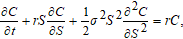
which is a partial differential equation, not a stochastic differential equation; the Black-Scholes formula is a solution to the Black-Scholes equation. It may be written as

$\begin{array}{}& C\left(S,K,\tau ,\sigma ,r\right)=\frac{1}{2\pi }\left(S{\int }_{-\infty }^{d_1}{e}^{-\frac{1}{2}{y}^2}\mathrm{dy}-{\mathrm{Ke}}^{-r\tau }{\int }_{-\infty }^{d_2}{e}^{-\frac{1}{2}{y}^2}\mathrm{dy}\right),\end{array}$

where

$\begin{array}{cc}{d}_1& =\frac{\ln (S/{\mathrm{Ke}}^{-r\tau })+(1/2){\sigma }^2\tau }{\sigma \sqrt{\tau }}\\ d_2& =\frac{\ln (S/{\mathrm{Ke}}^{-r\tau })-(1/2){\sigma }^2\tau }{\sigma \sqrt{\tau }}.\end{array}$

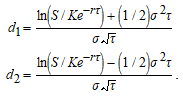
Here K is the strike price of the option, and τ is the time to expiration; these arise as constants of integration, fixed by the boundary conditions of the problem.

3. The Volatility Smile

When the BSM formula was first published in 1973, options trading was a small, unsystematic business. There was no widely accepted method for pricing options and little understanding of their value. In this context, the BSM formula had a natural application: it could be used to calculate the “fair” options price C, using options parameters K and τ, market values S and r, and one’s expectations about (or historical values of) σ. This calculation could then provide a baseline against which market prices might be compared, so that one could identify options that were over- or underpriced. This strategy was profitable until the early 1980s, by which time market prices aligned with BSM prices (MacKenzie Reference MacKenzie2006), meaning that comparatively little advantage could be gained merely by using the BSM formula.

Around this time, a second application of the BSM formula emerged. The idea behind this application was to effectively invert the formula: use market values for C, S, and r to compute σ. The idea is that some of the parameters going into the BSM formula are readily observable: either they are parameters governing the option under consideration, such as K and τ, or else they are market prices, such as C, S, and r. But the future volatility of the underlying asset is not observable. Inverting the BSM formula allows one to compute this unobservable quantity from observable quantities. The value so computed is known as implied volatility.

Implied volatility turns out to be useful. It provides some insight into market expectations concerning the future volatility of an asset. It also relativizes the price of an option to other (evolving) quantities, including the price of the underlying asset and the strike price of the option. For this reason, it provides a useful substitute for price, encoding information about how expensive an option is relative to other quantities of interest. (Briefly, the higher the implied volatility, the more expensive the option.) Options traders regularly quote implied volatilities to one another when describing trades.

But as useful as implied volatility is, it also leads to problems. In particular, the BSM model makes strong assumptions about the value of σ. In particular, σ appears in GBM as a (constant) parameter that characterizes the stochastic dynamics of the underlying asset and not any particular option written on that asset. It follows that σ must be independent of options parameters K and τ.

During the 1980s, when implied volatility was first used, it was (essentially) independent of K and τ, as expected. But following the October 19, 1987, market crash—a crash in which the BSM model was broadly implicated—options markets began to change (MacKenzie Reference MacKenzie2006; Derman and Miller Reference Derman and Miller2016). Traders began to notice a surprising relationship between the implied volatility of an option and the parameters characterizing that option. For a fixed time to expiration, options with strike prices far from the current price (i.e., options that would only be exercised if prices changed dramatically) now had higher implied volatilities. In other words, the more unlikely it was for an option to become valuable, the more expensive it became (as measured by the implied volatility). This anomalous behavior became known as the volatility smile.Footnote ⁷

The volatility smile was recognized as very strange. On its face, it suggests a contradiction in the BSM model—or, at least, between the BSM model and the results of this application.Footnote ⁸ The BSM model begins by assuming that a certain parameter has a constant value. From this assumption, one can derive a relationship—the BSM formula—between that parameter and some other market parameters. But on observing market conditions, one discovers—using the BSM formula—that the assumption underlying the formula does not hold, apparently undermining the formula with which the parameter was calculated. At the very least, the result of this analysis reveals that the relationship captured by the BSM formula does not accurately capture the relationship between future volatility, the price of the underlying asset, and the price of an option in real markets.

Nonetheless, traders continue to use the BSM model, or close descendants, for many purposes—including to calculate implied volatilities. The issue is not that the tension between the model’s assumptions and its output has gone unrecognized—to the contrary, it is well known. Influential derivatives modelers Derman and Miller sum it up as follows. “The existence of the smile poses a deep and interesting problem for option valuation, in both theory and practice. … The nonflat smiles [seen in real markets] tell us that actual option markets … violate the BSM model. Nevertheless, traders everywhere use implied BSM volatilities to quote options prices. … It’s strange and mysterious that markets use a model that doesn’t work to quote prices that deviate from it” (Derman and Miller Reference Derman and Miller2016, 133). Strange and mysterious indeed.

4. Why Use a Broken Model?

The upshot of the previous section is that there is a sense in which the BSM model is broken. And yet, the model continues to be used, despite this anomalous behavior. Worse, it is used for precisely the purposes that reveal its problems. What can account for this “strange and mysterious” practice?

In what follows, I present three attitudes that one might take to the volatility smile. Each of these attitudes occurs among traders and quantitative analysts, although I do not have any evidence for this aside from anecdotes from my own experience. (I do not claim that there are no other possible attitudes.)

The first attitude is the view that the BSM model is not broken after all; rather, the volatility smile is compatible with GBM, properly construed. I will call this attitude compatibilism. The idea is that one needs to draw an important distinction between (a) implied volatility, which measures what market participants expect about future volatility, and (b) actual volatility, which concerns the degree of variability that will in fact be exhibited by future returns.Footnote ⁹

It follows, on this attitude, that the volatility smile is not a strict contradiction. It is actual volatility that figures into GBM, whereas only implied volatility depends on the options parameters. Thus, one could accept all of the assumptions of the BSM model but take the volatility smile to show that market participants trading options with different parameters tend to have diverse beliefs about future volatility. It is also possible that various facts about supply and demand for options with various parameters have distorted market values, say because some traders are willing to pay an extra premium.

Compatibilism is probably tenable, and the core insight, that there is not a strict contradiction, is surely correct. But the further view that the BSM model is not “broken” has some unattractive features. For instance, one way to make sense of the position is to adopt a view of probability according to which there is a fact about the distribution of the random variable from which future market returns will be drawn.Footnote ¹⁰ GBM then implies that this must be a normal distribution with some given time-dependent variance, σ ²t, where σ is the parameter appearing in the BSM formula. The compatibilist must then say that although there is some fact about what value this parameter takes, market participants generally disagree about it. In other words, the BSM model is not incoherent, but it also is not very useful, because it requires one to know something that is (apparently) very difficult to accurately determine.

This broad disagreement about σ reflected in the volatility smile can be interpreted in another way: one might think that the volatility smile is incompatible with a single value of σ because market participants generally do not believe there is any value of σ that correctly reflects future returns. In other words, market participants generally reject GBM and the BSM model along with it. Of course, an individual compatibilist can accept this and even continue to use the BSM model because she happens to disagree with other market participants. But this cannot account for the widespread use of the model, since after all, the whole point would be that most traders believe the BSM model to be broken.

But if this is right, why is the BSM model still widely used? One answer reflects a second possible attitude toward the model, which I will call the trading zone (TZ) attitude.Footnote ¹¹ According to this attitude, one might accept that the BSM model makes incorrect assumptions about the probabilities of future returns and, therefore, should not be taken to provide reliable guidance on the relationship between options prices and other market parameters. Nonetheless, one might think that the model’s conceptual framework is still useful for reasoning about and discussing options.

One reason to think the BSM model remains useful is that it draws attention to market parameters that turn out to be relevant to options pricing, even if the relationship between them captured by the BSM formula is not correct. These include obvious parameters—such as the price of the underlying asset—but also less obvious parameters, such as the various partial derivatives appearing in equation (1). Indeed, these partial derivatives—known as the Greeks, for the letters used to denote them—are widely used by traders and analysts for evaluating possible trades.

Picking out salient parameters is particularly valuable in this context, because even though there seems to be broad agreement that the BSM model is incorrect, there is no universally accepted alternative. This means that while traders use many different models, they may nonetheless communicate with one another using the language of the BSM model. Moreover, many firms take the details of their (proprietary) models to have value that would be compromised if the models were revealed. But options traders and analysts often need to communicate with traders at other firms in order to execute trades. The BSM model, including the Greeks, provides a firm-independent baseline that traders and brokers can use to communicate, without revealing private information. This provides a strong reason to continue to use the BSM model—particularly for purposes such as quoting implied volatility as a substitute for price—even though everyone agrees that it fails in important cases.

The TZ attitude provides one answer for why the BSM model continues to be widely used, even if most market participants reject it. But there is a second, different answer to the same question that is in many ways more interesting. On this view, which I will call the informativist attitude, although one accepts that the BSM model is broken, one nonetheless takes the volatility smile to provide useful information. By studying, for a particular option, the way in which the BSM model fails—as reflected by the implied volatility curves associated with that option—one can (in the presence of some further assumptions) extract information about, for instance, market expectations about future probabilities. The BSM model again acts as a kind of baseline, not for communicating across different firms but relative to which actual market conditions can be evaluated.

To see how this works, observe that the BSM model ultimately delivers, as the “fair” price of an option, the price at which the future-discounted expected payoff of the option vanishes (i.e., the price at which it is as likely to be profitable as not). To calculate that expected payoff, one needs to assume some probability distribution for future returns on the underlying asset. That assumption is buried in GBM, which as I have noted implies that this distribution will be normal with variance σ ²t.

Now, as we saw above, GBM plays an essential role in the BSM argument, since it is this assumption that permits one to invoke Ito’s lemma and derive a risk-free portfolio. But there are reasons to doubt GBM. In particular, although one can fit historical returns to a normal distribution to extract an estimate for σ, generally the fit is not very good.Footnote ¹² Empirical returns for many assets are better fit to distributions with nonvanishing skew and excess kurtosis. Moreover, the qualitative feature of the volatility smile suggests that market participants tend to expect future returns to also have these properties. Generic volatility smiles reveal that options that are less likely to be profitable are comparatively more expensive, indicating that traders assign higher probability to those events than indicated if returns were normally distributed.

Suppose, then, that we took the basic framework of the BSM model for granted, but we understood the future returns of the underlying asset to be sampled from some other, presumably nonnormal, distribution. We could then ask, given this alternative distribution, what the “fair” price of an option would be. If one were to consider a range of options whose prices were calculated in this way, and derive (BSM) implied volatilities from those prices, one would generically find implied volatility to vary with strike price. In other words, the volatility smile would arise if market participants believed the true distribution over future returns was nonnormal. Moreover, the shape of the volatility smile produced in this way would reflect properties of the probability distribution used to calculate the prices, in a fairly direct way: the curvature of the smile (i.e., its second derivative) would vary proportionately to the excess kurtosis, and the skew (or first derivative) of the smile would vary with the skew of the probability distribution.

Reasoning in the other direction, then, one might infer from the volatility smiles in real markets information about what likelihoods market participants, taken in aggregate, assign to certain future events. In fact, the volatility smile may generally be used to derive an implied (nonnormal) distribution for returns on the underlying asset (Breeden and Litzenberger Reference Breeden and Litzenberger1978; Hull Reference Hull2009; Derman and Miller Reference Derman and Miller2016).Footnote ¹³ This is detailed, often tradeable information that probes market expectations about the probabilities for specific ranges of returns and that would be very difficult to acquire otherwise. And the crucial point is that one gets that information from the BSM model only because the BSM model breaks down.

5. Conclusion

I have now presented the BSM model and the unexpected pattern (i.e., the volatility smile) that one finds when one uses it to calculate implied volatility. I have described why the volatility smile appears to contradict the very model used to calculate it, and I have presented three attitudes that one might take toward the volatility smile that could explain why one would nonetheless continue to use the BSM model. These attitudes are not necessarily incompatible—in particular, one could certainly accept both the trading zone attitude and the informativist attitude—but they do track importantly different considerations, any of which could explain individual traders continuing to use the BSM model despite the volatility smile.

The first attitude—compatibilism—reflects a quotidian picture of why one might use a model: because one thinks its assumptions accurately (or approximately) capture the situation one is interested in. But the situation with the other two attitudes is different. By adopting either TZ or informativism one continues to use a model that one believes to fail, in precisely the domain where it does fail. On TZ, one does so because the BSM model can still be helpful in facilitating reasoning and communicating about options, even without accurately capturing the relationships of interest. This attitude seems to best explain the use of implied volatilities as a substitute for price: implied volatility effectively encodes price relative to other parameters, in a way that does not require one to divulge private information. On the informativist attitude, meanwhile, one actively exploits the model’s failures to extract new information about other market participants. In this way, the BSM model, by virtue of how it fails, provides a new kind of tool for understanding markets.

This third attitude suggests some important morals concerning the role of (un)realistic assumptions in economic modeling. There is a long debate, going back to Friedman (Reference Friedman1953), concerning whether the standard assumptions in economic models—rational agents, efficient markets, and so on—are sufficiently realistic to support reliable inferences about, for instance, policy interventions.Footnote ¹⁴ Recent work has focused on the idea that false assumptions are used to “isolate” the true causal structure or relations operative in some phenomenon of interest from other less relevant factors.Footnote ¹⁵ The idea is that a model can be “realistic” in the sense of accurately representing essential features or capacities of some economic system, even though many of the assumptions in the model are false, because the role of those assumptions is to circumscribe the target of the model.

I do not want to argue that false assumptions do not often play this role in economic thought.Footnote ¹⁶ But they do not do so in the BSM model, at least on the informativist attitude. There, the false assumption—GBM, which implies normality of returns—concerns precisely what is essential to the model; it does not allow one to “isolate” other more essential features of options prices.Footnote ¹⁷ Worse, it is the failure of this assumption that makes the BSM model inadequate, or “unrealistic,” as a model of options prices. For these reasons, it is very difficult to see the widespread use of BSM implied volatilities as an instance of focusing on some essential feature of markets that is accurately reflected by the model. Indeed, the failure of GBM implies that volatility, as conceived by the model, is not a feature of markets at all.

So what does the BSM model do, and what role does the false assumption play? Ultimately, the informativist uses the BSM model to measure the manner in which GBM fails.Footnote ¹⁸ This suggests that bad assumptions do not always lead to useless models, even when the bad assumptions concern essential features the model’s target. To the contrary, false assumptions can serve as a probe for identifying better assumptions. If the isolationist credo might be fairly sloganized as, “false assumptions generate true(er) models,” then the BSM model suggests that in some cases the opposite is true: “false models can generate true(er) assumptions.”

There is a connection here to debates in philosophy of physics, concerning whether certain idealizations are “essential” or whether they play a merely pragmatic role. Bob Batterman has long argued that some idealizations are essential for the purposes to which the models using those idealizations are put, precisely because it is the circumstances under which an idealized model breaks down that provides the most valuable output. For instance, he writes: “we [should] rethink the use of models in physics. If we include mathematical features as essential parts of physical modeling then we will see that blowups or singularities are often sources of information” (Batterman Reference Batterman2011, 1038). The current example is different in many details from the examples he considers, which generally involve singular behavior near critical points and applications of renormalization group theory. But I think it is similar in spirit: it is because the BSM model fails that it turns out to be so useful.Footnote ¹⁹