



1. Introduction
Turbulent drag reduction technology holds significant engineering value in reducing energy consumption for fluid transport systems and enhancing marine vehicle propulsive efficiency. In recent years, superhydrophobic surfaces (SHS), leveraging slip boundary effects induced by solid–gas interfaces, have emerged as a novel approach to reduce wall shear stress substantially (Busse & Sandham Reference Busse and Sandham2012; Busse et al. Reference Busse, Sandham, McHale and Newton2013; Xia Reference Xia2024). The drag reduction mechanism primarily stems from slip conditions attenuating velocity gradients, altering near-wall vortex structures and modifying turbulent fluctuation energy transport processes (Jouin et al. Reference Jouin, Cherubini and Robinet2024). However, practical applications face challenges such as interfacial pressure fluctuations and surface roughness heterogeneity, which compromise the stability of gas–liquid interfaces and lead to discontinuities in slip boundaries (Rothstein Reference Rothstein2010). Existing studies predominantly focus on idealised continuous slip models, while the synergistic evolution between turbulent dynamics and drag reduction under discontinuous slip conditions remains insufficiently understood.
In idealised stable conditions, Rastegari & Akhavan (Reference Rastegari and Akhavan2015) proposed that the substantial drag reduction of SHS primarily stems from dual mechanisms. The first and dominant contribution arises from the gas–liquid interfacial slip, quantified as the ratio of the mean slip velocity to the bulk velocity, which originates from the reduction of the mean velocity gradient at the wall. The second mechanism involves the modulation of turbulent coherent structures, a contribution that typically accounts for no more than 20
 $\,\%$
of the total drag reduction and may even induce drag enhancement under spanwise slip conditions. Türk et al. (Reference Türk, Daschiel, Stroh, Hasegawa and Frohnapfel2014) demonstrated that at small groove spacings, drag reduction matches laminar predictions and is dominated by slip, whereas larger spacings excite coherent streamwise vortices that significantly enhance turbulence modulation. The turbulence-modulation mechanisms of slip boundaries are multifaceted: elevating near-wall vortex structures to reduce energy dissipation (Martell et al. Reference Martell, Rothstein and Perot2010), suppressing streamwise vortices and turbulent streaks to diminish turbulent transport (Park et al. Reference Park, Sun and Kim2014), disrupting the spanwise and streamwise scales of turbulence eddies (Teo & Khoo Reference Teo and Khoo2010; Hokmabad & Ghaemi Reference Hokmabad and Ghaemi2017). This competition between slip-induced benefits and turbulence-modulation effects is strongly regulated by the surface’s anisotropic micro-geometry, as evidenced in regular SHS with longitudinal grooves. Specifically, Park et al. (Reference Park, Choi and Kim2021) demonstrated that for a given gas fraction, longitudinal groove configurations achieve superior drag reduction performance compared with micropost structures by leveraging anisotropic slip, characterised by a significantly enhanced streamwise-slip length and a suppressed spanwise slip. Watanabe et al. (Reference Watanabe, Mamori and Fukagata2017) investigated SHS with various groove orientations, revealing that increased spanwise slip and weakened streamwise slip significantly degrade drag reduction performance. High-resolution particle image velocimetry (PIV) measurements by Li et al. (Reference Li, Ji, Tan, Li, Xiang, Lv and Duan2020) showed that drag reduction over a liquid–gas interface in turbulent boundary-layer flow increases with the friction Reynolds number (
 ${\textit{Re}}_\tau$
). Their drag-decomposition analysis traced this increase mainly to the growth of the dimensionless slip velocity (
 $U_s/U_b$
), with turbulence-related modifications remaining secondary in their measurements. While these studies establish the physical ingredients of continuous or periodically textured slip boundaries, they do not yet clarify how a prescribed slip/no-slip discontinuity reorganises drag decomposition, near-wall boundary-layer re-equilibration and turbulence transport in channel flow.
As the critical near-wall vortex dynamics are challenging to resolve experimentally and are inadequately captured by the Reynolds-averaged Navier–Stokes method or large eddy simulation, direct numerical simulation (DNS) is widely regarded as the benchmark high-fidelity approach. When conducting DNS of flow over SHS, two modelling strategies are commonly adopted: one approach explicitly resolves the microscale geometry and texture of the SHS, yielding the highest physical fidelity, while the extremely fine mesh required to resolve microscale features entails substantial computational cost; the alternative is to represent the surface microstructure by equivalent macroscopic boundary conditions, which preserves the leading-order macroscopic effects while markedly reducing numerical expense. Seo et al. (Reference Seo, García-Mayoral and Mani2017) model SHS as alternating slip/no-slip boundaries, and describe dynamic gas–liquid interface deformation by incorporating a linearised Young–Laplace equation, to couple the interfacial dynamics with turbulent flows. They ultimately demonstrate that the coherent structures in the overlying flow induced by interface fluctuations are significantly smaller in scale, and interface deformation alters neither the mean nor the fluctuations of the velocity profiles in turbulent statistics. Jelly et al. (Reference Jelly, Jung and Zaki2014) modelled SHS using a flat interface with alternating slip and no-slip boundaries, identifying a reduction in turbulent kinetic energy (TKE) production and revealing that the skin friction on the no-slip regions of the SHS exceeds that of a reference no-slip surface. Consequently, the flat gas–liquid interface assumption has been widely adopted as a computationally efficient and reliable strategy for DNS focusing on macroscopic flow features (Park et al. Reference Park, Park and Kim2013; Fairhall et al. Reference Fairhall, Abderrahaman-Elena and García-Mayoral2018). In the present study we adopt this macroscopic modelling framework and do not resolve the microscale interface texture. Further simplification is achieved by employing a spatially averaged macroscopic Navier-slip boundary condition:
 \begin{equation} \begin{aligned} u_s = l_s^u \frac {\partial u}{\partial y} \Big|_{\textit{wall}}, \quad w_s = l_s^w \frac {\partial w}{\partial y} \Big|_{\textit{wall}} \end{aligned} \end{equation}
to model SHS. This formulation couples the streamwise and spanwise slip velocity components (
 $u_s$
,
 $w_s$
) to the instantaneous local velocity gradients at the wall via the slip length
 $l_s$
, effectively parameterising the surface’s effect and reducing computational complexity. Extensive studies demonstrate that this model achieves excellent agreement with theoretical predictions in laminar flows (Davis & Lauga Reference Davis and Lauga2010; Li et al. Reference Li, Alame and Mahesh2017), and produces the same mean velocity profiles and root-mean-square velocity fluctuations as those of heterogeneous slip/no-slip boundaries in turbulent flows (Seo et al. Reference Seo, García-Mayoral and Mani2015; Seo & Mani Reference Seo and Mani2016; Seo et al. Reference Seo, García-Mayoral and Mani2017). Notably, it also predicts slip-induced instability mode transitions in laminar-turbulent transitional flow (Min & Kim Reference Min and Kim2005; Picella et al. Reference Picella, Robinet and Cherubini2019, Reference Picella, Robinet and Cherubini2020).
When the flow encounters abrupt changes in boundary conditions, near-wall momentum transport and turbulent structures reorganise across multiple scales, manifesting as sharp peaks or sudden drops in wall shear stress or skin-friction coefficient and producing pronounced changes in the velocity field and the Reynolds-stress distribution (Antonia & Luxton Reference Antonia and Luxton1971a , Reference Antonia and Luxtonb ; Andreopoulos & Wood Reference Andreopoulos and Wood1982; Rouhi et al. Reference Rouhi, Chung and Hutchins2019). In practical SHS applications, slip/no-slip discontinuities often arise from manufacturing defects or flow-induced interface instabilities; however, the effects of such discontinuous slip boundaries on near-wall flow-field re-equilibration and overall drag reduction performance remain insufficiently explored. In this study we assume that the SHS features periodic spanwise no-slip stripes are arranged along the streamwise direction, and we systematically investigate the influence of these discontinuous slip boundaries on channel flow characteristics and drag reduction efficacy. This specific configuration is representative of scenarios like periodic mechanical support ribs used to reinforce superhydrophobic textures (Wang et al. Reference Wang2020) or transverse assembly joints in segmented drag-reducing skins (Bixler & Bhushan Reference Bixler and Bhushan2013).
The remainder of the paper is organised as follows. In § 2 the numerical methods and computational domain are detailed. In § 3 the main results are presented, focusing on: (i) the decomposition of drag reduction contributions and the effects of slip patterns, (ii) the mechanism of boundary-layer re-equilibration induced by the no-slip stripe, and (iii) the modulation of TKE budgets. Finally, conclusions are summarised in § 4.
2. Computational methodology
2.1. Problem formulation
Figure 1 schematically illustrates the three representative configurations investigated in the present study, which comprise a continuous boundary, a discontinuous slip boundary with a single no-slip stripe per period and a discontinuous slip boundary containing multiple no-slip stripes per period. A Cartesian coordinate system is employed with its origin
 $(x, y, z) = (0, 0, 0)$
situated at the streamwise centre of the channel on the bottom wall, and the axes
 $x$
,
 $y$
and
 $z$
denote the streamwise, wall-normal and spanwise directions, respectively. The computational domain has dimensions
 $L_x\times L_y\times L_z=2\pi \delta \times 2\delta \times \pi \delta$
, where
 $\delta$
is the channel half-height,
 $L_x$
is the streamwise periodic length,
 $L_y$
is the channel height and
 $L_z$
is the spanwise periodic length. The adequacy of this domain size is supported by two-point autocorrelation analysis, which shows negligible streamwise velocity correlation at half-domain lengths in both the streamwise and spanwise directions, and by the results of Lozano-Durán & Jiménez (Reference Lozano-Durán and Jiménez2014), who showed that a domain of the same size captures more than 95 % of the Reynolds-stress production even at substantially higher
 ${\textit{Re}}_\tau$
. Periodic boundary conditions are applied in the homogeneous
 $x$
and
 $z$
directions. The upper and lower walls are applied with the Navier-slip boundary condition for the continuous slip cases, while the walls are prescribed with alternating slip regions and no-slip stripes of width
 $d$
and streamwise pitch
 $\lambda =L_x/n$
for the discontinuous slip cases, where
 $n$
denotes the number of no-slip stripes within
 $L_x$
. In the slip regions, the tangential velocity is formulated as
 \begin{equation} \begin{aligned} u-l_s^u\frac {\partial u}{\partial y}=0, \quad w-l_s^w\frac {\partial w}{\partial y}=0, \end{aligned} \end{equation}
where
 $l_s^u$
and
 $l_s^w$
denote the streamwise and spanwise slip lengths, respectively. The condition
 $l_s^u = l_s^w \equiv l_s$
is prescribed for the isotropic cases, while anisotropic cases are examined separately to isolate the role of the spanwise slip component. A Dirichlet boundary condition,
 $u=v=w=0$
, is prescribed on the no-slip stripe regions. The specific cases and simulation parameters are summarised in table 1. The no-slip case is used as the reference no-slip channel flow at
 ${\textit{Re}}_b=6988$
, for which
 ${\textit{Re}}_\tau \approx 395$
, and the no-slip-HR case is used as the corresponding high-Reynolds-number reference case at
 ${\textit{Re}}_b=13976$
(
 ${\textit{Re}}_\tau \approx 725$
). Here,
 ${\textit{Re}}_\tau =u_\tau \delta /\nu$
is the friction Reynolds number,
 ${\textit{Re}}_b = u_b \delta / \nu$
is the bulk Reynolds number based on the bulk velocity
 $u_b$
,
 $u_\tau =\sqrt {\tau _w/\rho }$
is the friction velocity,
 $\nu$
is the kinematic viscosity,
 $\tau _w$
is the wall shear stress and
 $\rho$
is the fluid density. Cases Val-Cs-180 (
 ${\textit{Re}}_b = 2739$
,
 ${\textit{Re}}_\tau = 180$
) and Val-Ns-395 (
 ${\textit{Re}}_b = 6988$
,
 ${\textit{Re}}_\tau = 395$
) are employed for numerical validation against the benchmark data of Min & Kim (Reference Min and Kim2004) and for grid convergence, respectively. To evaluate the flow characteristics and drag reduction performance, the remaining cases are categorised into three groups: (i) isotropic continuous and discontinuous slip boundaries with varying
 $L_s=l_s/\delta$
(in viscous units,
 $L_s^+ = l_s u_{\tau 0}/\nu$
ranges from 1.977 to 7.908); (ii) isotropic discontinuous slip boundaries with different geometries (wider
 $d$
or smaller
 $\lambda$
) of no-slip stripes; and (iii) anisotropic continuous and discontinuous slip boundaries with a fixed
 $L_s^u=l_s^u/\delta$
and varying
 $L_s^w=l_s^w/\delta$
. Here,
 $L_s$
, encompassing the streamwise-slip length
 $L_s^u$
and the spanwise slip length
 $L_s^w$
, represents the dimensionless slip length scaled by
 $\delta$
, and is adopted as the standard notation throughout the remainder of this study. Furthermore,
 $L_s^+$
, including
 $(L_s^u)^+$
and
 $(L_s^w)^+$
, in table 1, denotes an alternative representation scaled by viscous wall units
 $u_{\tau 0}$
(Min & Kim Reference Min and Kim2004). For most cases in the parameter study, the bulk Reynolds number is fixed at
 ${\textit{Re}}_b=6988$
under a constant mass-flow-rate condition, and the resulting
 ${\textit{Re}}_\tau$
varies with the boundary condition. In addition, a corresponding high-Reynolds-number comparison is performed at
 ${\textit{Re}}_b=13976$
for the no-slip reference and the two
 $L_s=0.01$
slip cases.
Schematic of the computational domain and representative surface configurations considered in the present study. (
 $a$
) Reference no-slip channel flow. (
 $b$
) Discontinuous slip boundary with
 $n=1$
spanwise no-slip stripe per streamwise period, where the upper and lower walls consist of alternating slip regions and the no-slip stripe (shaded areas), and periodic boundary conditions are imposed in the streamwise and spanwise directions. Here
 $x_{ns}$
and
 $x_{ps}$
represent the streamwise coordinates of the leading and trailing edges of the no-slip stripe, respectively. (
 $c$
) Discontinuous slip boundary with
 $n=2$
no-slip stripes per streamwise period, characterised by stripe width
 $d$
and streamwise pitch
 $\lambda =L_x/n$
.

Summary of simulation parameters for all cases studied. The cases are grouped into four categories. Here
 $(L_s^u)^+$
and
 $(L_s^w)^+$
denote the streamwise and spanwise slip lengths normalised by the viscous length scale
 $\nu /u_{\tau 0}$
of the corresponding no-slip reference case. The nomenclature is defined as follows: ‘HR’ denotes the high Reynolds number (i.e.
 ${\textit{Re}}_b = 13976$
); ‘Val’ denotes validation cases; ‘Cs’ and ‘Ds’ represent continuous and discontinuous slip boundaries, respectively, with ‘Ls’ specifying the slip length magnitude; ‘D’ and ‘
 $\lambda$
’ indicate stripe width
 $d$
and pitch
 $\lambda$
, respectively; ‘AiCs’ and ‘AiDs’ denote anisotropic continuous and discontinuous slip boundaries, with ‘Lu’ and ‘Lw’ indicating the streamwise and spanwise slip lengths, respectively.

Table 1. Long description
The table presents simulation parameters for different cases grouped into four categories. It has 26 rows and 10 columns. Column headers are Group, Case, Ls_s^u & Ls_s^w, (Ls_s^u)^+ & (Ls_s^w)^+, λ/δ, d/δ, Reb, and Reτ. Row labels include Reference cases and numerical validation, Isotropic continuous and discontinuous slip cases with Ls variation and high-Reynolds-number comparison, Isotropic discontinuous slip boundaries with different geometries of no-slip stripes, and Anisotropic continuous and discontinuous slip boundaries with a fixed Ls_s^u = 0.01 and varying Ls_s^w. Each row lists specific values for the parameters, providing a detailed comparison across different cases.
2.2. Numerical method
In the present study, DNS of fully developed turbulent channel flow are performed under a constant mass flow rate. The governing equations are the non-dimensional incompressible Navier–Stokes equations:
 \begin{align} \frac {\partial \boldsymbol{u}}{\partial t}+\boldsymbol{u}\boldsymbol{\cdot }\boldsymbol{\nabla }\boldsymbol{u}&=\boldsymbol{f}-\boldsymbol{\nabla }p+\frac {1}{{\textit{Re}}_b}{\nabla} ^2\boldsymbol{u}, \end{align}
 \begin{align} \boldsymbol{\nabla }\boldsymbol{\cdot }\boldsymbol{u}&=0. \end{align}
Here
 $\boldsymbol{u}=(u,v,w)$
is the velocity and
 $p(x,y,z,t)$
is the pressure normalised by the liquid density. The velocity components,
 $u$
,
 $v$
and
 $w$
are in the
 $x$
,
 $y$
and
 $z$
directions, respectively, normalised by
 $u_b$
, and the viscous term is written in terms of
 ${\textit{Re}}_b$
. A spatially uniform body force is applied in the
 $x$
direction to maintain the prescribed flow rate. The computations are carried out using a spectral/hp element method (SEM) embedded in an open source code, Nektar++ (Cantwell et al. Reference Cantwell2015; Du et al. Reference Du, Gao, You, Chen, Liu, Li, Lv and Duan2024). A quasi-three-dimensional solution strategy is adopted to solve the three-dimensional Navier–Stokes equations: the governing equations are spatially discretised by the spectral-element method in the (
 $x$
,
 $y$
)-plane, while a Fourier expansion is used in the
 $z$
direction to recover the full three-dimensional flow field. Concretely, the two-dimensional mesh comprises
 $N_x=32$
equally spaced
 $h$
-type elements in
 $x$
, and
 $N_y=32$
 $h$
-type elements in
 $y$
with wall-normal grid refinement realised via a hyperbolic-tangent stretching function. Within each
 $h$
-type element, a
 $p$
-type spectral refinement is applied with polynomial interpolation order
 $N_p$
. The
 $z$
direction is represented by a Fourier modal expansion comprising
 $N_z=192$
modes. To mitigate pressure oscillations, the velocity components (
 $u$
,
 $v$
,
 $w$
) and pressure (
 $p$
) are discretised with distinct
 $N_p$
, and numerical integration and evaluation of the nonlinear terms are performed via the Gauss–Lobatto–Legendre method. The spatial resolution parameters for each case are listed in table 1. The time integration employed a second-order implicit-explicit scheme, and the spectral vanishing viscosity (SVV) diffusion coefficient is set as 0.1 to improve numerical stability (Moura et al. Reference Moura, Aman, Peiró and Sherwin2020). To quantify statistical convergence, the simulation time is reported using the eddy turnover time
 $t_{et}=\delta /u_{\tau 0}$
, where
 $u_{\tau 0}$
denotes the friction velocity of the reference no-slip case. Specifically, the simulations are first run for more than
 $10\,t_{et}$
to achieve fully developed turbulence, and then for more than an additional
 $5\,t_{et}$
to obtain statistically converged time-averaged drag coefficients and flow statistics.
Numerical validation is performed against two benchmark datasets: the reference no-slip channel flow (No-slip) is compared with Lee & Moser (Reference Lee and Moser2015), and the continuous slip validation case (Val-Cs-180) at
 ${\textit{Re}}_{\tau }\approx 180$
and
 $L_s=0.01$
is compared with Min & Kim (Reference Min and Kim2004). The results show excellent agreement, as illustrated in figure 2. The spatial resolution in the wall-parallel directions is
 $\Delta x^+\approx 11$
and
 $\Delta z^+\approx 5.5$
. The non-uniform mesh in the wall-normal direction has a minimum size
 $\Delta y_{{min}}^+\approx 0.8$
at the wall and a maximum size
 $\Delta y_{{\textit{max}}}^+\approx 3.2$
at the channel centre. Grid convergence of the simulations is assessed separately by comparing the baseline no-slip case (No-slip) at polynomial orders
 $N_p=$
7 and 6 with the validation case (Val-Ns-395) at higher orders
 $N_p=$
9 and 8, where the former
 $N_p$
value in each pair represents velocity components (
 $u$
,
 $v$
,
 $w$
) and the latter represents pressure (
 $p$
). The comparison shows excellent agreement in the dimensionless spatio-temporally averaged velocity
 $\langle \bar {u}\rangle ^+$
(scaled by
 $u_\tau$
) and root-mean-square velocity
 $\boldsymbol{u}_{\textit{rms}}=\langle \overline {{\boldsymbol{u}^\prime }^2}\rangle ^{0.5}/u_{\tau 0}$
profiles, with maximum discrepancy below 3 %. Throughout the remainder of the paper, the instantaneous velocity
 $\boldsymbol{u}(x, y, z, t)$
is decomposed as
 $\boldsymbol{u} = \bar {\boldsymbol{u}} + \boldsymbol{u}^\prime$
, where
 $\bar {\boldsymbol{u}}(x, y, z)$
denotes the time-averaged velocity and
 $\boldsymbol{u}^\prime (x, y, z, t)$
represents the fluctuating component. The overbar
 $\bar {\boldsymbol{\cdot }}$
signifies time averaging and the angle bracket
 $\langle \boldsymbol{\cdot }\rangle$
denotes spatial averaging in the streamwise and spanwise directions. Subscripts ‘
 $x$
’ or ‘
 $z$
’ are used to indicate averaging in the streamwise or spanwise directions, respectively, when spatial averaging is applied only in one direction (e.g. in §§ 3.1, 3.2, 3.4 and 3.5). Consequently, all cases excluding Val-Ns-395 employ
 $N_p=$
7 and 6 for the polynomial expansion in the simulations.
Validation of the spatio-temporally averaged streamwise velocity
 $\langle \bar {u}\rangle ^+$
(scaled by
 $u_\tau$
) profiles as a function of the wall-normal distance
 $y^+$
(scaled by
 $\nu /u_\tau$
). The present DNS results for the no-slip channel flow (No-slip) at
 ${\textit{Re}}_{\tau }=395$
are compared with the benchmark data of Lee & Moser (Reference Lee and Moser2015), and the results for the continuous slip channel flow (Val-Cs-180) with
 $L_{s}=0.01$
at
 ${\textit{Re}}_{\tau }=180$
are compared with Min & Kim (Reference Min and Kim2004).

3. Results and discussion
3.1. Analysis on decomposition of drag reduction contributions
To elucidate the fundamental physical mechanisms governing the alterations in drag reduction and turbulence statistics induced by periodic transverse no-slip stripes, a double-averaging (DA) methodology is implemented (Raupach & Shaw Reference Raupach and Shaw1982). This framework enables a triple decomposition of the instantaneous velocity
 $\boldsymbol{u}$
into three constituent parts: (i) a spatio-temporally averaged (DA) component
 $\langle \bar {\boldsymbol{u}}\rangle$
, (ii) a dispersive component
 $\tilde {\boldsymbol{u}}=\bar {\boldsymbol{u}}-\langle \bar {\boldsymbol{u}}\rangle$
, representing stationary spatial fluctuations induced by surface heterogeneity, and (iii) a stochastic turbulent fluctuation
 $\boldsymbol{u}^\prime =\boldsymbol{u}-\bar {\boldsymbol{u}}$
. The resulting triple decomposition is expressed as
 \begin{equation} \boldsymbol{u}(x,y,z,t) = \langle \bar {\boldsymbol{u}}\rangle (y) + \tilde {\boldsymbol{u}}(x,y,z) + \boldsymbol{u}^\prime (x,y,z,t). \end{equation}
The DA operator is defined as the average over both the wall-parallel plane area
 $A=L_x\times L_z$
and the integration time
 $T$
:
 \begin{equation} \langle \bar {\boldsymbol{u}}\rangle (y) = \frac {1}{AT}\iint _{t}\int _{A}\boldsymbol{u}(x,y,z,t)\text {d}A\text {d}t. \end{equation}
Due to the continuity equation and the wall-impermeability condition, the DA component of the wall-normal velocity vanishes (
 $\langle \bar {v}\rangle = 0$
). Consequently, the nonlinear convective term
 $\langle \bar {u}\bar {v}\rangle$
can be expanded as
 \begin{equation} \langle \bar {u}\bar {v}\rangle =\langle (\langle \bar {u}\rangle +\tilde {u})\tilde {v}\rangle =\langle \bar {u}\rangle \langle \tilde {v}\rangle +\langle \tilde {u}\tilde {v}\rangle =\langle \tilde {u}\tilde {v}\rangle , \end{equation}
where
 $-\langle \tilde {u} \tilde {v} \rangle$
is the dispersive shear stress (Jelly & Busse Reference Jelly and Busse2018), representing the momentum transport contribution from stationary spatial fluctuations induced by boundary heterogeneity.
Comparison of wall-normal profiles of mean flow statistics for no-slip, continuous slip and discontinuous slip boundaries at various
 $L_s$
. (
 $a$
) Mean velocity
 $\langle \bar {u}\rangle ^+$
. (
 $b$
) Root-mean-square velocity fluctuations
 $\boldsymbol{u}_{\textit{rms}} = \langle \overline {{u_i^\prime }^2}\rangle ^{0.5}/u_{\tau 0}$
. (
 $c$
) Shear stress
 $\langle \tau \rangle ^{+0}$
components: viscous shear stress
 $\langle \tau _\nu \rangle ^{+0}$
and Reynolds shear stress
 $-\langle \tau _R\rangle ^{+0}$
. (
 $d$
) Dispersive shear stress
 $-\langle \tilde {u}\tilde {v}\rangle ^+$
. Solid lines denote the discontinuous slip cases (Ds-Ls005, Ds-Ls010, Ds-Ls020), with a fixed no-slip stripe configuration (
 $d/\delta = \pi /8, \lambda /\delta = 2\pi$
) and the no-slip reference flow (No-slip). Dashed lines denote the corresponding continuous slip cases (Cs-Ls005, Cs-Ls010, Cs-Ls020) at the same
 $L_s$
. The black arrows indicate the direction of increasing
 $L_s$
.

Figure 3. Long description
The image contains four panels, each depicting a different type of graph related to mean flow statistics for no-slip, continuous slip, and discontinuous slip boundaries. Panel A shows a line graph of mean velocity profiles. The x-axis is labeled y+ and the y-axis is labeled <u+>. The graph includes multiple lines representing different conditions: no-slip, Ds-Ls005, Cs-Ls005, Ds-Ls010, Cs-Ls010, Ds-Ls020, and Cs-Ls020. Panel B shows a line graph of root-mean-square velocity fluctuations. The x-axis is labeled y+0 and the y-axis is labeled (u_i^2)^0.5/u_tau0. The graph includes lines for u_rms, v_rms, and w_rms under different conditions. Panel C shows a line graph of shear stress components. The x-axis is labeled y+0 and the y-axis is labeled <tau_v>+0 and -<tau_R>+0. The graph includes lines representing different conditions. Panel D shows a line graph of dispersive shear stress. The x-axis is labeled y+ and the y-axis is labeled -<u’v’>+. The graph includes lines for different conditions. The black arrows in each panel indicate the direction of increasing slip length.
The macroscopic effects of continuous and discontinuous slip boundaries on the mean flow statistics are initially examined. Figure 3 compares the spatio-temporally averaged profiles of mean velocity
 $\langle \bar {u}\rangle ^+$
, root-mean-square velocity fluctuations (i.e. turbulence intensity)
 $\boldsymbol{u}_{\textit{rms}}=\langle \overline {{\boldsymbol{u}^\prime }^2}\rangle ^{0.5}/u_{\tau 0}$
, shear stress
 $\langle \tau \rangle ^{+0}$
components (the superscript ‘
 $+0$
’ signifies normalisation by
 $u_{\tau 0}$
such that
 $\langle \tau \rangle ^{+0}=\langle \tau \rangle /u_{\tau 0}^2$
), and the dispersive shear stress
 $-\langle \tilde {u}\tilde {v}\rangle ^+ = -\langle \tilde {u}\tilde {v}\rangle /u_\tau ^2$
for turbulent channel flows over continuous and discontinuous slip boundaries across different
 $L_s$
with a fixed no-slip stripe width
 $d$
and pitch
 $\lambda$
. The imposition of slip boundary conditions effectively relaxes the kinematic wall constraint, leading to a monotonic upward displacement of both the dimensionless slip velocity
 $u_s^+=u_s/u_\tau$
and the mean velocity
 $\langle \bar {u}\rangle ^+$
profile relative to the no-slip reference flow, an observation that aligns with the benchmark findings of Min & Kim (Reference Min and Kim2004). At larger slip lengths (e.g.
 $L_s=0.01$
and 0.02), the introduction of the no-slip stripe induces an appreciable downward shift in the
 $\langle \bar {u}\rangle ^+$
profile, indicating a localised momentum deficit induced by the surface heterogeneity. As shown in figure 3(
 $b$
), within the viscous sublayer (
 $y^{+0}=yu_{\tau 0}/\nu \lt 5$
), the spatio-temporally averaged turbulence intensities are enhanced with
 $L_s$
in the continuous slip cases, and are further increased in the discontinuous slip cases. This amplification stems from the combined effects of the release of the wall constraint and the excitation of shear-layer instabilities by the no-slip stripe. In the logarithmic layer (
 $y^{+0}\gt 30$
), all three components of turbulence intensity decrease with
 $L_s$
in the discontinuous slip cases, but are enhanced compared with the continuous slip cases. Figure 3(
 $c$
) shows the profiles of the spatio-averaged Reynolds shear stress (
 $\langle \tau _R\rangle ^{+0}=-\langle \overline {u^\prime v^\prime }\rangle /u_{\tau 0}^2$
) and viscous shear stress (
 $\langle \tau _\nu \rangle ^{+0}=\nu \langle \partial \bar {u} / \partial y \rangle /u_{\tau 0}^2$
). In the continuous slip boundary flows, increasing
 $L_s$
leads to a decrease in the peak
 $\langle \tau _R\rangle ^{+0}$
and the wall values of
 $\langle \tau _\nu \rangle ^{+0}$
, but the no-slip stripe weakens this decreasing trend. As illustrated in figure 3(
 $d$
), the introduction of the no-slip stripe induces spatial heterogeneity at the top and bottom boundaries, which gives rise to dispersive shear stress
 $-\langle \tilde {u}\tilde {v}\rangle ^+$
in the near-wall region (
 $y^+\lt 30$
, covering the viscous sublayer and the buffer layer) of the discontinuous slip configurations. Furthermore, the magnitude of
 $-\langle \tilde {u}\tilde {v}\rangle ^+$
increases progressively with
 $L_s$
.
Comparison of wall-normal profiles of mean flow statistics for continuous slip and discontinuous slip boundaries at various
 ${\textit{Re}}_\tau$
. (
 $a$
) Mean velocity
 $\langle \bar {u}\rangle ^+$
. (
 $b$
) Root-mean-square velocity fluctuations
 $\boldsymbol{u}_{\textit{rms}} = \langle \overline {{u_i^\prime }^2}\rangle ^{0.5}/u_{\tau 0}$
. (
 $c$
) Shear stress
 $\langle \tau \rangle ^{+0}$
components: viscous shear stress
 $\langle \tau _\nu \rangle ^{+0}$
and Reynolds shear stress
 $-\langle \tau _R\rangle ^{+0}$
(no-slip and no-slip-HR cases are included for reference). (
 $d$
) Dispersive shear stress
 $-\langle \tilde {u}\tilde {v}\rangle ^+$
. Solid lines denote the discontinuous slip cases (Ds-Ls010, Ds-Ls010-HR), and the no-slip reference flow (No-slip, No-slip-HR). Dashed lines denote the corresponding continuous slip cases (Cs-Ls010, Cs-Ls010-HR).

To examine the Reynolds number dependence of the flow statistics discussed above,
 ${\textit{Re}}_b$
is increased from
 ${\textit{Re}}_b=6988$
to
 ${\textit{Re}}_b=13976$
for the no-slip reference and the two slip cases (Cs-Ls010, Ds-Ls010) with
 $L_s=0.01$
, raising
 ${\textit{Re}}_\tau$
of the no-slip reference from
 ${\textit{Re}}_\tau \approx 395$
to
 ${\textit{Re}}_\tau \approx 725$
. The high-Reynolds-number slip cases use the same slip length (
 $L_s=0.01$
) and the same no-slip stripe geometry (
 $\lambda /\delta =2\pi$
,
 $d/\delta =\pi /8$
) as their low-Reynolds-number counterparts, so that any differences can be attributed to the change in Reynolds number rather than to a change in the surface parameters. Figure 4 compares the spatio-temporally averaged wall-normal profiles of
 $\langle \bar {u}\rangle ^{+}$
,
 $\boldsymbol{u}_{\textit{rms}}$
,
 $\langle \tau \rangle ^{+0}$
and
 $-\langle \tilde {u}\tilde {v}\rangle ^+$
at the two Reynolds numbers. For the high-Reynolds-number slip cases, the normalisation with
 $u_{\tau 0}$
uses the friction velocity of the no-slip-HR reference case. As shown in figure 4(
 $a$
),
 $\langle \bar {u}\rangle ^+$
shift upward with increasing
 ${\textit{Re}}_\tau$
, reflecting the larger
 $u_s^+$
obtained at the higher
 ${\textit{Re}}_b$
for a fixed
 $L_s$
, as also reported in the PIV measurements of Li et al. (Reference Li, Ji, Tan, Li, Xiang, Lv and Duan2020). Figure 4(
 $b$
) shows that
 $\boldsymbol{u}_{\textit{rms}}$
is only weakly affected by
 ${\textit{Re}}_\tau$
:
 $u_{\textit{rms}}$
and
 $w_{\textit{rms}}$
increase slightly in the viscous sublayer, while the buffer-layer values of
 $u_{\textit{rms}}$
and
 $v_{\textit{rms}}$
decrease marginally. Figure 4(
 $c$
) shows that
 $\langle \tau _\nu \rangle ^{+0}$
decreases with
 ${\textit{Re}}_\tau$
, and the reduction of
 $-\langle \tau _R\rangle ^{+0}$
becomes less pronounced at high
 ${\textit{Re}}_\tau$
. Figure 4(
 $d$
) shows that the dispersive shear stress
 $-\langle \tilde {u}\tilde {v}\rangle ^+$
increases in both peak magnitude and wall-normal extent, although it remains a minor contribution to the overall stress balance. Overall, an analysis of the flow phenomenology reveals that the influence of the no-slip stripe on the mean flow characteristics is only weakly dependent on the Reynolds number.
Following the solution strategy of Rastegari & Akhavan (Reference Rastegari and Akhavan2015), the streamwise momentum equation is spatio-temporally averaged and integrated along the wall-normal direction using the generalised FIK (Fukagata–Iwamoto–Kasagi) identity (Fukagata et al. Reference Fukagata, Iwamoto and Kasagi2002), yielding the total friction coefficient
 $C_{\!f}$
:
 \begin{equation} C_{\!f} = \frac {6}{{\textit{Re}}_b}\left (1 - \frac {u_s}{u_b}\right ) + 3C_{\!f} \int _0^1 (1-\xi ) \left [ -\langle \overline {u'v'}\rangle ^+ - \langle \tilde {u}\tilde {v}\rangle ^+ \right ] {\rm d}\xi. \end{equation}
Here
 $C_{\!f} = 2\langle u_\tau \rangle ^2 / u_b^2$
and
 $\xi = y/\delta$
denotes the dimensionless wall-normal coordinate. Through reformulation, the total friction coefficient can be expressed as
 \begin{equation} C_{\!f} = \frac {6}{{\textit{Re}}_b}\left (1 - \frac {u_s}{u_b}\right ) \left [ \frac {1}{1 - 3(I_{\textit{turb}}^+ + I_{\textit{disp}}^+)} \right ], \end{equation}
where the turbulent and dispersive integrals,
 $I_{\textit{turb}}^+$
and
 $I_{\textit{disp}}^+$
, are defined respectively as
 \begin{align} I_{\textit{turb}}^+ &= \int _0^1 (1-\xi ) \left [ -\langle \overline {u^\prime v^\prime }\rangle ^+ \right ] {\rm d}\xi , \nonumber\\ I_{\textit{disp}}^+ &= \int _0^1 (1-\xi ) \left [ -\langle \tilde {u}\tilde {v}\rangle ^+ \right ] {\rm d}\xi . \end{align}
The drag reduction is defined as
 $DR = (C_{\!f}^0 - C_{\!f}) / C_{\!f}^0$
, where
 $C_{\!f}^0$
denotes the friction coefficient for the no-slip reference case. Accordingly, the total drag reduction for discontinuous slip boundaries can be partitioned into three physical contributions:
 \begin{equation} \begin{aligned} {\textit{DR}}_{\textit{total}} = \underbrace { \frac {u_s}{u_b} }_{{\textit{DR}}_s} + \underbrace { \left (1 - \frac {u_s}{u_b}\right ) \frac {3\left(I_{\textit{turb}}^{+0} - I_{\textit{turb}}^+\right)}{1 - 3\left(I_{\textit{turb}}^+ + I_{\textit{disp}}^+\right)} }_{{\textit{DR}}_{\textit{turb}}} + \underbrace { \left (1 - \frac {u_s}{u_b}\right ) \frac {-3I_{\textit{disp}}^+}{1 - 3\left(I_{\textit{turb}}^+ + I_{\textit{disp}}^+\right)} }_{{\textit{DR}}_{\textit{disp}}}. \end{aligned} \end{equation}
Here,
 ${\textit{DR}}_s$
denotes the drag reduction arising from the slip contribution,
 ${\textit{DR}}_{\textit{turb}}$
represents the effect of turbulence modulation and
 ${\textit{DR}}_{\textit{disp}}$
represents the contribution of dispersive momentum transport, induced by stationary spatial fluctuations associated with the non-uniform slip/no-slip boundary, to the total drag variation, typically manifesting as a drag penalty;
 $I_{\textit{turb}}^{+0} = \int _0^1 (1-\xi ) [ -\langle \overline {u'v'}\rangle ^{+0} ] {\rm d}\xi$
is defined as the turbulent integral under the no-slip reference case.
Decomposition of the total drag reduction
 ${\textit{DR}}_{\textit{total}}$
as a function of
 $L_s$
. The total drag reduction
 ${\textit{DR}}_{\textit{total}}$
(
 $\diamond$
) is partitioned into the slip-induced contribution
 ${\textit{DR}}_s$
(
 $\circ$
), the turbulence-modulation contribution
 ${\textit{DR}}_{\textit{turb}}$
(
 $\square$
) and the dispersive penalty
 ${\textit{DR}}_{\textit{disp}}$
(
 $\triangle$
) arising from surface heterogeneity. Results are compared between the discontinuous slip cases (Ds-Ls005, Ds-Ls010, Ds-Ls020) and the corresponding continuous slip cases (Cs-Ls005, Cs-Ls010, Cs-Ls020).

Figure 5. Long description
Panel: A line graph depicts the decomposition of total drag reduction as a function of slip length. The horizontal axis represents slip length (L subscript s) in unspecified units, ranging from 0.005 to 0.020. The vertical axis represents drag reduction (D R) in percent, ranging from -5 percent to 35 percent. The graph includes four data series: D R subscript s (slip-induced contribution) represented by circles and a solid yellow line, D R subscript turb (turbulence-modulation contribution) represented by squares and a dashed light blue line, D R subscript disp (dispersive penalty) represented by triangles and a dashed dark blue line, and D R subscript total (total drag reduction) represented by diamonds and a dashed black line. The graph is divided into two regions: discontinuous slip and continuous slip. In the discontinuous slip region, D R subscript s increases from approximately 10 percent to 30 percent as slip length increases. D R subscript turb remains close to zero, with slight negative values. D R subscript disp also stays near zero. D R subscript total follows a similar trend to D R subscript s, peaking around 30 percent. In the continuous slip region, D R subscript s decreases from approximately 30 percent to 10 percent as slip length decreases. D R subscript turb and D R subscript disp remain near zero. D R subscript total decreases accordingly, mirroring the trend of D R subscript s.
Figure 5 compares the partition of the total drag reduction
 ${\textit{DR}}_{\textit{total}}$
into the slip-induced contribution
 ${\textit{DR}}_s$
, the turbulence-modulation contribution
 ${\textit{DR}}_{\textit{turb}}$
and the dispersive penalty
 ${\textit{DR}}_{\textit{disp}}$
for turbulent channel flows over continuous and discontinuous slip boundaries at various
 $L_s$
. Consistent with the reduced slip velocity shown in figure 3(
 $a$
),
 ${\textit{DR}}_s$
for discontinuous boundaries is attenuated relative to the continuous case. The magnitude of this attenuation exhibits an approximately linear scaling with
 $L_s$
, increasing from 0.72
 $\,\%$
at
 $L_s=0.005$
to 2.72
 $\,\%$
at
 $L_s=0.02$
. This behaviour reflects the dynamical response in the small-slip limit (
 $L_s \ll \delta$
), where the modulation of the wall velocity gradient by the slip velocity constitutes a first-order perturbation, thus rendering
 $u_s$
linearly dependent on
 $L_s$
. Meanwhile, isotropic slip induces a drag penalty within the turbulence-modulation term at low
 $L_s$
(
 $=0.005$
and 0.01), a detrimental effect that is further exacerbated by the no-slip stripe. Conversely, the slip boundary enhances a beneficial modulation effect at high
 $L_s$
(
 $=0.02$
), but this gain is suppressed by the localised disturbances triggered by the no-slip stripe. The underlying mechanism involves a competition between two opposing near-wall effects. The streamwise-slip component is beneficial, acting to stabilise low-speed streaks and weaken the turbulence-regeneration cycle. Conversely, the spanwise slip component is detrimental, permitting a lateral ‘stirring’ motion that enhances the transport efficiency of quasi-streamwise vortices, strengthens ejection/sweep events, and thus, increases Reynolds shear stress. For isotropic slip boundaries, the outcome of this competition depends on
 $L_s$
: at low slip lengths the detrimental ‘stirring’ dominates, yielding a net drag increase, whereas at high
 $L_s$
the beneficial stabilising effect prevails, resulting in a net drag reduction. This trend is consistent with the simulations of Rastegari & Akhavan (Reference Rastegari and Akhavan2015) on SHS made of isotropic micropillars, which are effectively regarded as the isotropic continuous slip boundaries employed in this study. The dispersive penalty
 ${\textit{DR}}_{\textit{disp}}$
exerts a considerably smaller impact on
 ${\textit{DR}}_{\textit{total}}$
compared with the other two components. Here
 ${\textit{DR}}_{\textit{disp}}$
introduces a progressive drag penalty in the discontinuous configurations that increases with
 $L_s$
, while it vanishes for homogeneous continuous slip boundaries, consistent with figure 3(
 $d$
). This contribution originates from the enhancement of dispersive shear stresses induced by the prescribed surface heterogeneity (i.e. the no-slip stripe).
Decomposition of the total drag reduction
 ${\textit{DR}}_{\textit{total}}={\textit{DR}}_s+{\textit{DR}}_{\textit{turb}}+{\textit{DR}}_{\textit{disp}}$
for the continuous and discontinuous
 $L_s=0.01$
slip cases at the two bulk Reynolds numbers.

Table 2. Long description
A table with four rows and seven columns comparing drag reduction for continuous and discontinuous slip cases at two bulk Reynolds numbers. The columns are labeled Case, Reb, Reτ, DRs, DRturb, DRdisp, and DRtotal. The rows are labeled with different cases: Cs-Ls010, Ds-Ls010, Cs-Ls010-HR, and Ds-Ls010-HR. Each row provides specific values for each column, detailing the decomposition of total drag reduction. Notable trends include variations in DRs, DRturb, DRdisp, and DRtotal across different cases and Reynolds numbers.
Table 2 presents the decomposition of
 ${\textit{DR}}_{\textit{total}}$
for the continuous and discontinuous slip cases at the two Reynolds numbers. At the higher Reynolds number,
 ${\textit{DR}}_{\textit{total}}$
increases markedly for both boundary types, mainly because of the increase in
 ${\textit{DR}}_s$
. This trend is consistent with the larger
 $u_s^+$
observed in figure 4(
 $a$
). The turbulence-modulation contribution changes from a small drag penalty at low
 ${\textit{Re}}_\tau$
to a drag-reducing contribution at high
 ${\textit{Re}}_\tau$
, indicating a Reynolds-number-dependent shift in the balance between spanwise-slip-induced lateral stirring and streamwise-slip-induced turbulence attenuation. Although the prescribed slip length remains
 $L_s=0.01$
, its value in wall units (
 $L_s^+$
) increases to a level comparable to the low-Reynolds-number cases with
 $L_s=0.02$
(table 1). This stronger near-wall slip, characterised by a larger
 $u_s^+$
, shifts
 $\langle \bar {u}\rangle ^+$
profile upward and more effectively reduces turbulent momentum transport relative to the no-slip reference, enabling the stabilising streamwise slip to overcome the spanwise penalty. The dispersive contribution
 ${\textit{DR}}_{\textit{disp}}$
becomes slightly more negative for the discontinuous case at high
 ${\textit{Re}}_b$
, consistent with the stronger stationary spatial fluctuations shown in figure 4(
 $d$
), but its magnitude remains much smaller than those of
 ${\textit{DR}}_s$
and
 ${\textit{DR}}_{\textit{turb}}$
. At both Reynolds numbers, introducing the no-slip stripe reduces
 ${\textit{DR}}_{\textit{total}}$
relative to the corresponding continuous slip case. This reduction is dominated by the decrease in
 ${\textit{DR}}_s$
, because the no-slip region reduces the effective slip area, while the additional reduction in
 ${\textit{DR}}_{\textit{turb}}$
and the small dispersive penalty provide secondary corrections. Thus, the Reynolds number changes the magnitude of drag reduction, whereas the qualitative impact of the no-slip stripe is unchanged in this matched comparison.
Streamwise distribution of spanwise-temporally averaged wall quantities for discontinuous slip boundary channel flow with
 $L_s=0.005$
, 0.01 and 0.02 (corresponding to Ds-Ls005, Ds-Ls010 and Ds-Ls020). (
 $a$
) Dimensionless wall pressure
 $\langle \bar {p}\rangle _z^+$
and (
 $b$
) local friction velocity
 $u_{\tau ,w}^{+0}$
at
 $y^+=0$
are plotted as functions of the normalised streamwise coordinate
 $x/\delta$
.

Figure 6. Long description
Two line graphs depict the streamwise distribution of spanwise-temporally averaged wall quantities for discontinuous slip boundary channel flow. Panel A: The line graph shows dimensionless wall pressure as a function of the normalized streamwise coordinate. The x-axis is labeled x/δ and the y-axis is labeled p+. The graph includes three lines representing different values of discontinuous slip boundary conditions: Ds-Ls005, Ds-Ls010, and Ds-Ls020. The APG (Adverse Pressure Gradient) and FPG (Favorable Pressure Gradient) regions are marked. The lines show significant fluctuations around the x/δ value of 0, with peaks and troughs indicating changes in wall pressure. Panel B: The line graph shows local friction velocity at y+ as a function of the normalized streamwise coordinate. The x-axis is labeled x/δ and the y-axis is labeled uτ,ω+. The graph includes the same three lines representing different values of discontinuous slip boundary conditions: Ds-Ls005, Ds-Ls010, and Ds-Ls020. The lines show fluctuations around the x/δ value of 0, with peaks and troughs indicating changes in local friction velocity.
The streamwise distribution of spanwise-temporally averaged wall pressure
 $\langle \bar {p}\rangle _z^+$
(scaled by
 $\rho u_b^2$
) for the discontinuous slip boundary is illustrated in figure 6(
 $a$
). The result confirms the emergence of a sharp localised pressure peak at the leading edge of the no-slip stripe, followed by a rapid pressure drop to a relatively low level across the stripe interior and a minimum at the trailing edge. Consequently, significant adverse pressure gradient (APG) regions develop upstream of the no-slip stripe’s leading edge and downstream of its trailing edge, while a strong favourable pressure gradient (FPG) prevails throughout the stripe interior. Figure 6(
 $b$
) presents the streamwise distribution of
 $u_{\tau ,w}^{+0}=u_{\tau ,w}/u_{\tau 0}$
, where
 $u_{\tau ,w}(x)=[\nu (\partial \langle \bar {u}\rangle _z/\partial y)]^{0.5}|_{y=0}$
denotes the spanwise-averaged local friction velocity. A dramatic overshoot of the local wall shear stress manifests at the leading edge of the no-slip stripe, where
 $u_{\tau ,w}$
surges to a peak value significantly higher than the equilibrium level. This behaviour arises because the high-speed fluid from the slip region abruptly encounters the no-slip constraint at the leading edge of the no-slip stripe, promoting the formation of low-speed attached vortices there. Following this peak,
 $u_{\tau ,w}$
decays rapidly within the stripe and gradually recovers in the subsequent slip region. As the flow leaves the no-slip stripe and re-enters the downstream slip region, the corresponding re-adjustment near the trailing edge also contributes to the vortical structures observed downstream of the stripe. These pressure gradient and wall-shear signatures indicate that the no-slip stripe introduces strong localised disturbances near the slip/no-slip transitions.
For examining the associated vortical response, instantaneous vortical structures are identified via the
 $Q$
-criterion, defined as
 $Q=(\|\varOmega \|^2-\|S\|^2)/2$
, where
 $\varOmega =[(\partial u_i/\partial x_{\!j})-(\partial u_j/\partial x_i)]/2$
and
 $S=[(\partial u_i/\partial x_{\!j})+(\partial u_j/\partial x_i)]/2$
represent the antisymmetric vorticity tensor and the symmetric strain-rate tensor, respectively.
Three-dimensional isosurfaces of vortical structures by the
 $Q$
-criterion (
 $Q^{+0} = 0.01$
) for discontinuous slip boundaries at (
 $a$
)
 $L_s=0.005$
(Ds-Ls005), (
 $b$
)
 $L_s=0.01$
(Ds-Ls010), and (
 $c$
)
 $L_s=0.02$
(Ds-Ls020), where the colour indicates the dimensionless streamwise velocity magnitude
 $u/u_b$
ranging from 0 to 1.2. The blue arrows represent the leading edges of the no-slip stripes, while the red arrows represent their trailing edges. Wall-normal profiles of (
 $d$
)
 $\langle \bar {f}_Q\rangle$
, (
 $e$
)
 $\langle \overline {Q^{+0}\boldsymbol{\cdot }f_Q}\rangle$
, and (
 $f$
)
 $\langle \overline {Q^{+0}\boldsymbol{\cdot }f_Q}\rangle /\langle \bar {f}_Q\rangle$
for no-slip, continuous slip and discontinuous slip boundaries at various
 $L_s$
. Solid lines denote the discontinuous slip cases and the no-slip reference flow. Dashed lines denote the corresponding continuous slip cases at the same
 $L_s$
.

The instantaneous vortical structures are visualised in figure 7(
 $a-c$
) using isosurfaces of the
 $Q$
-criterion with a threshold of
 $Q^{+0}=Q/(u_{\tau 0}^4/\nu ^2)=0.01$
, coloured by the dimensionless streamwise velocity magnitude
 $u/u_b$
. The value
 $Q^{+0}=0.01$
is selected as the isosurface threshold for visualising rotation-dominated vortical structures, consistent with the threshold levels used in previous turbulent channel and superhydrophobic channel flow studies (Watanabe et al. Reference Watanabe, Mamori and Fukagata2017; Nakamura et al. Reference Nakamura, Fukami, Hasegawa, Nabae and Fukagata2021). This threshold provides clear and comparable isosurfaces across the present cases while avoiding excessive visual obstruction at lower
 $Q$
values. Shear-layer instability is triggered within the two localised APG regions, promoting the generation and bursting of small-scale turbulent structures and thereby producing low-speed attached vortices near the leading and trailing edges of the no-slip stripe. Meanwhile, suppression of turbulence intensity by slip reduces the total population of vortical structures as
 $L_s$
increases.
To further quantify the effects of the no-slip stripe and
 $L_s$
on the intensity and distribution characteristics of vortical structures, an instantaneous threshold-window indicator for vortical events is defined over the interval
 $0.005 \lt Q^{+0} \lt 0.05$
as
 \begin{equation} f_Q(x,y,z,t)= \int _{0.005}^{0.05} \delta _D\!\left (q-Q^{+0}(x,y,z,t)\right )\,\mathrm{d}q . \end{equation}
Here,
 $\delta _D$
denotes the Dirac delta function, so the integral acts as an indicator:
 $f_Q=1$
when the local value of
 $Q^{+0}$
lies within this interval and
 $f_Q=0$
otherwise. The wall-normal profile
 $\langle \bar {f}_Q\rangle (y)$
is then obtained by applying the same wall-parallel plane and time average defined above. The interval
 $0.005\lt Q^{+0}\lt 0.05$
is used as a threshold-window statistic around the visualisation level
 $Q^{+0}=0.01$
, covering weaker-to-stronger rotation-dominated events while excluding very weak near-zero events. This choice follows the same order-of-magnitude practice as previous thresholded vortex-criterion statistics in superhydrophobic channel flows, where comparable ranges have been used to evaluate vortex-core probability density functions and population density (Jelly et al. Reference Jelly, Jung and Zaki2014). Figure 7(d–f) present the wall-normal profiles of the event probability
 $\langle \bar {f}_Q\rangle$
, the
 $Q^{+0}$
-weighted event intensity
 $\langle \overline {Q^{+0} f_Q}\rangle$
and the conditional mean intensity
 $\langle \overline {Q^{+0} f_Q}\rangle / \langle \bar {f}_Q\rangle$
for the continuous and discontinuous slip cases as well as the no-slip reference at various
 $L_s$
with fixed
 $d$
and
 $\lambda$
. As shown in figure 7(
 $d,e$
), the peak of
 $\langle \bar {f}_Q\rangle$
appears in the buffer layer, consistent with Jelly et al. (Reference Jelly, Jung and Zaki2014), and the distribution density of vortical structures decreases with increasing
 $L_s$
. Owing to the generation of near-wall low-speed attached vortices by the no-slip stripe,
 $\langle \bar {f}_Q\rangle$
in the viscous sublayer of the discontinuous slip cases is no longer zero and increases slightly with
 $L_s$
. Furthermore, as illustrated in figure 7(
 $f$
), the mean vortex intensity in the viscous sublayer of the discontinuous slip boundaries increases significantly with
 $L_s$
. At
 $L_s=0.02$
, the regions near the leading and trailing edges of the no-slip stripe even become the locations of maximum vortex intensity in the flow field, while the vortex intensity in the buffer layer decreases with increasing
 $L_s$
. Consequently, the drag increase within the turbulence-modulation contribution induced by discontinuous slip boundaries is primarily driven by two mechanisms: the turbulent vortex events triggered by the localised APG and the intense frictional drag penalty resulting from the concentration of local shear stress. Furthermore, the pronounced spatial heterogeneity in the local velocity field, induced by the heterogeneous wall-pressure and friction-velocity distributions, accounts for the emergence of the dispersive shear stress. This provides a comprehensive physical explanation for the degradation of drag reduction performance on discontinuous slip boundaries.
3.2. Effects of no-slip stripe geometries on flow features and drag reduction
To systematically investigate how no-slip stripe geometries modulate the flow statistics and drag reduction of discontinuous slip boundaries, a parametric study is conducted along two paths: (i) fixing the pitch at
 $\lambda /\delta = 2\pi$
while increasing the stripe width
 $d$
(cases Ds-Ls010-D0.25
 $\pi$
, Ds-Ls010-D0.50
 $\pi$
and Ds-Ls010-D1.00
 $\pi$
); and (ii) fixing the stripe width at
 $d/\delta = \pi /8$
while decreasing the pitch
 $\lambda$
(cases Ds-Ls010-
 $\lambda$
1.00
 $\pi$
, Ds-Ls010-
 $\lambda$
0.50
 $\pi$
and Ds-Ls010-
 $\lambda$
0.25
 $\pi$
). All subsequent analyses employ the case with
 $d/\delta = \pi /8$
and
 $\lambda /\delta = 2\pi$
(Ds-Ls010) as the reference baseline, aiming to resolve the differential contributions of the streamwise distribution density of surface heterogeneity and the localised disturbance intensity to the turbulent statistical features and drag reduction performance.
Comparison of wall-normal profiles of mean flow statistics for different no-slip stripe geometries (
 $d$
and
 $\lambda$
) at a fixed
 $L_s=0.01$
. (
 $a$
) Mean velocity with the slip velocity subtracted,
 $\langle \bar {u}\rangle ^+-u_s^+$
. (
 $b$
) Root-mean-square velocity fluctuations
 $\boldsymbol{u}_{\textit{rms}} = \langle \overline {{u_i^\prime }^2}\rangle ^{0.5}/u_{\tau 0}$
. (
 $c$
) Shear stress
 $\langle \tau \rangle ^{+0}$
components: viscous shear stress
 $\langle \tau _\nu \rangle ^{+0}$
and Reynolds shear stress
 $-\langle \tau _R\rangle ^{+0}$
. (
 $d$
) Dispersive shear stress
 $-\langle \tilde {u}\tilde {v}\rangle ^+$
. Solid lines denote the cases with increasing
 $d$
(Ds-Ls010-D0.25
 $\pi$
, Ds-Ls010-D0.50
 $\pi$
, Ds-Ls010-D1.00
 $\pi$
) at a fixed
 $\lambda /\delta =2\pi$
, along with the reference case (Ds-Ls010). Dashed lines denote the cases with decreasing
 $\lambda$
(Ds-Ls010-
 $\lambda$
1.00
 $\pi$
, Ds-Ls010-
 $\lambda$
0.50
 $\pi$
, Ds-Ls010-
 $\lambda$
0.25
 $\pi$
) at a fixed
 $d/\delta =\pi /8$
.

Figure 8. Long description
The image contains four panels, each depicting different aspects of wall-normal profiles of mean flow statistics for various no-slip stripe geometries. Panel A shows a line graph of the mean velocity with the slip velocity subtracted. The x-axis is labeled y+ and ranges from 10^0 to 10^2, while the y-axis is labeled <u+> - us+ and ranges from 0 to 20. The graph includes multiple lines representing different cases with increasing and decreasing Ds-Ls010 values. Panel B presents a line graph of root-mean-square velocity fluctuations. The x-axis is labeled y+0 and ranges from 0 to 100, while the y-axis is labeled (u_rms, v_rms, w_rms) / u_tau0 and ranges from 0 to 2.5. The graph shows three sets of lines for u_rms, v_rms, and w_rms, each representing different cases. Panel C displays a line graph of shear stress components. The x-axis is labeled y+0 and ranges from 0 to 100, while the y-axis is labeled <tau_v>+0 and <tau_R>+0 and ranges from -0.5 to 1.0. The graph includes lines for viscous shear stress and Reynolds shear stress, representing different cases. Panel D shows a line graph of dispersive shear stress. The x-axis is labeled y+ and ranges from 0 to 100, while the y-axis is labeled -<u’v’>+ and ranges from 0 to 20 x 10^-3. The graph includes multiple lines representing different cases with increasing and decreasing Ds-Ls010 values.
Figure 8 compares the spatio-temporally averaged profiles of
 $\langle \bar {u}\rangle ^{+}-u_s^+$
,
 $\boldsymbol{u}_{\textit{rms}}$
,
 $\langle \tau \rangle ^{+0}$
and
 $-\langle \tilde {u}\tilde {v}\rangle ^+$
under various no-slip stripe geometries. As illustrated in figure 8(
 $a$
), increasing
 $d$
and decreasing
 $\lambda$
lead to an elevated no-slip area fraction
 $d/\lambda$
, which subsequently reduces
 $u_s^+$
. With constant
 $d/\lambda$
, reducing
 $\lambda$
attenuates
 $u_s^+$
more significantly than increasing
 $d$
. This trend is primarily attributed to the proliferation of local APG regions and the inter-stripe non-equilibrium interference. At small
 $\lambda$
(e.g.
 $\lambda /\delta =\pi /4$
), the recovery process of the flow after traversing the no-slip constraint is truncated, forcing frequent flow-field re-equilibrations at the stripe edges and leading to an accumulated slip deficit. Furthermore, increasing
 $d$
and decreasing
 $\lambda$
thicken the buffer layer in the
 $\langle \bar {u}\rangle ^{+} - u_s^{+}$
profile. This finding is consistent with Rastegari & Akhavan (Reference Rastegari and Akhavan2015), where an increase in the slip area fraction was shown to thin the buffer layer; conversely, the increase in
 $d/\lambda$
observed in the present study leads to its thickening. As shown in figure 8(
 $b$
), increasing
 $d$
exerts a marginal influence on
 $u_{\textit{rms}}$
,
 $v_{\textit{rms}}$
and
 $w_{\textit{rms}}$
within the buffer and logarithmic layers, whereas decreasing
 $\lambda$
to
 $\lambda /\delta =0.25\pi$
(Ds-Ls010-
 $\lambda$
0.25
 $\pi$
) results in a significant enhancement of
 $u_{\textit{rms}}$
and
 $v_{\textit{rms}}$
because the inter-stripe interference maintains the flow in a non-equilibrium state and augments the turbulence intensity. Furthermore, both increasing
 $d$
and decreasing
 $\lambda$
lead to a reduction of
 $u_{\textit{rms}}$
and
 $v_{\textit{rms}}$
within the viscous sublayer, stemming from the expanded no-slip coverage, which imposes stronger kinematic constraints on the near-wall fluctuations. As illustrated in figure 8(
 $c$
), both increasing
 $d$
and decreasing
 $\lambda$
enhance
 $\langle \tau _\nu \rangle ^{+0}$
in the viscous sublayer and
 $\langle \tau _R\rangle ^{+0}$
in the logarithmic layer, with decreasing
 $\lambda$
exerting a more significant influence than increasing
 $d$
for a given
 $d/\lambda$
. The augmentation of
 $\langle \tau _R\rangle ^{+0}$
arises because a smaller
 $\lambda$
increases the frequency with which the fluid encounters the leading-edge discontinuity and the associated intense localised APG, where these high-frequency disturbances disrupt the near-wall momentum balance and trigger shear-layer instabilities and bursting events. The mechanism for the enhancement of
 $\langle \tau _\nu \rangle ^{+0}$
is consistent with the variations in
 $u_s$
, and its modifications are primarily confined to the near-wall region of
 $y^+ \le 8$
, confirming that no-slip stripes do not alter the core momentum transport mechanism in the far-wall region. As shown in figure 8(
 $d$
), increasing
 $d$
primarily extends the wall-normal penetration of surface heterogeneity into the flow field, causing the influence of the induced
 $-\langle \tilde {u}\tilde {v}\rangle ^+$
to expand from the viscous sublayer and buffer layer deep into the logarithmic layer. Specifically for
 $d/\delta = \pi$
(Ds-Ls010-D1.00
 $\pi$
), the effective range of the dispersive effect extends up to
 $y^+ \approx 60$
. In contrast, decreasing
 $\lambda$
predominantly affects the magnitude of
 $-\langle \tilde {u}\tilde {v}\rangle ^+$
by increasing the frequency of flow-field re-equilibration per unit streamwise length. This phenomenon indicates that
 $d$
governs the wall-normal penetration depth of surface heterogeneity induced disturbances, while the stripe density (the reciprocal of
 $\lambda$
) determines the energy intensity of such perturbations.
Figure 9(
 $a$
) illustrates the influence of varying no-slip stripe geometries on
 ${\textit{DR}}_{\textit{total}}$
and its constituent components
 ${\textit{DR}}_s$
,
 ${\textit{DR}}_{\textit{turb}}$
and
 ${\textit{DR}}_{\textit{disp}}$
at a fixed slip length
 $L_s = 0.01$
. Compared with the baseline Ds-Ls010 configuration, both increasing
 $d$
and decreasing
 $\lambda$
lead to an enhanced dispersive penalty manifested by an increase in the absolute value of
 ${\textit{DR}}_{\textit{disp}}$
, which is consistent with the expanded influence and magnitude of
 $-\langle \tilde {u}\tilde {v}\rangle ^+$
shown in figure 8(
 $d$
) and confirms that surface heterogeneity is a primary cause of additional momentum loss. Notably, increasing
 $d$
and decreasing
 $\lambda$
do not result in a linear reduction of
 ${\textit{DR}}_{\textit{turb}}$
due to the complex competition among the stabilising effect of streamwise slip, the lateral ‘stirring’ motion induced by spanwise slip, the localised flow response inducing attached vortices and the non-equilibrium inter-stripe interference. For cases with increasing
 $d$
at fixed
 $\lambda$
(corresponding to increasing
 $d/\lambda$
), the effective boundary condition progressively approaches the no-slip limit, thereby weakening the modulation of turbulent coherent structures and causing
 ${\textit{DR}}_{\textit{turb}}$
to vanish gradually. In contrast, the effect of decreasing
 $\lambda$
on
 ${\textit{DR}}_{\textit{turb}}$
exhibits a distinct non-monotonicity governed by inter-stripe interference, where at larger
 $\lambda$
the stripes remain independent and decreasing
 $\lambda$
merely causes the flow to approach the no-slip reference; whereas at smaller
 $\lambda$
such as Ds-Ls010-
 $\lambda$
0.25
 $\pi$
, the flow frequently traverses the alternating slip and no-slip boundaries, and the flow field perpetually remains in a non-equilibrium state, which vigorously excites near-wall turbulent structures to further decrease
 ${\textit{DR}}_{\textit{turb}}$
, thereby increasing drag.
Decomposition of
 ${\textit{DR}}_{\textit{total}}$
as a function of no-slip stripe geometries (
 $d$
and
 $\lambda$
). (
 $a$
) The
 ${\textit{DR}}_{\textit{total}}$
(
 $\diamond$
) is partitioned into
 ${\textit{DR}}_s$
(
 $\circ$
),
 ${\textit{DR}}_{\textit{turb}}$
(
 $\square$
) and
 ${\textit{DR}}_{\textit{disp}}$
(
 $\triangle$
). Results are compared among the leftward discontinuous slip cases with increasing
 $d$
(Ds-Ls010-D0.25
 $\pi$
, Ds-Ls010-D0.50
 $\pi$
, Ds-Ls010-D1.00
 $\pi$
), the rightward cases with decreasing
 $\lambda$
(Ds-Ls010-
 $\lambda$
1.00
 $\pi$
, Ds-Ls010-
 $\lambda$
0.50
 $\pi$
, Ds-Ls010-
 $\lambda$
0.25
 $\pi$
) and the reference case (Ds-Ls010). (
 $b$
) Comparison of the actual
 ${\textit{DR}}_s$
with theoretical predictions considering the slip area deficit only (the dashed line), and the combined effects of slip area deficit and localised flow-field re-equilibration (the dash-dotted line).

Figure 10(a–c) presents the instantaneous coherent vortex topologies for the no-slip reference and the representative extreme cases Ds-Ls010-D1.00
 $\pi$
and Ds-Ls010-
 $\lambda$
0.25
 $\pi$
, while panels (d–f) display the wall-normal profiles of
 $\langle \bar {f}_Q\rangle$
,
 $\langle \overline {Q^{+0}\boldsymbol{\cdot }f_Q}\rangle$
and
 $\langle \overline {Q^{+0}\boldsymbol{\cdot }f_Q}\rangle / \langle \bar {f}_Q\rangle$
for discontinuous slip cases with different no-slip stripe geometries at a fixed
 $L_s=0.01$
and the reference no-slip case. As shown in figure 10(
 $d,e$
), increasing
 $d$
at fixed
 $\lambda$
elevates
 $\langle \bar {f}_Q\rangle$
in the buffer and logarithmic layers, driving the vortical structure field of the discontinuous slip cases progressively toward the no-slip baseline, which explains why
 ${\textit{DR}}_{\textit{turb}}$
vanishes gradually as
 $d$
increases. However, varying
 $d$
does not affect the distribution density of vortical structures within the viscous sublayer, because the number of no-slip stripes per streamwise period,
 $n$
, remains unchanged, so the localised APG regions and the associated low-speed attached vortices do not increase (see figure 10
 $b$
). By contrast, decreasing
 $\lambda$
at fixed
 $d$
increases
 $n$
, which markedly raises the population density of low-speed vortices in the viscous sublayer (see figure 10
 $c$
). Furthermore, as illustrated in figure 10(
 $f$
), the mean vortex intensity over the entire flow field remains insensitive to variations in stripe geometry, indicating that the geometric characteristics of no-slip stripes primarily modulate the spatial distribution density rather than the intrinsic intensity of vortical structures.
Three-dimensional isosurfaces of vortical structures using
 $Q^{+0} = 0.01$
for (
 $a$
) the reference no-slip case (No-slip) and discontinuous slip cases at a fixed
 $L_s=0.01$
with (
 $b$
)
 $d/\delta =\pi$
,
 $\lambda /\delta =2\pi$
(Ds-Ls010-D1.00
 $\pi$
), and (
 $c$
)
 $d/\delta =\pi /8$
,
 $\lambda /\delta =\pi /4$
(Ds-Ls010-
 $\lambda$
0.25
 $\pi$
). The colour indicates the dimensionless streamwise velocity magnitude
 $u/u_b$
ranging from 0 to 1.2. The blue arrows represent the leading edges of the no-slip stripes, while the red arrows represent their trailing edges. Wall-normal profiles of (
 $d$
)
 $\langle \bar {f}_Q\rangle$
, (
 $e$
)
 $\langle \overline {Q^{+0}\boldsymbol{\cdot }f_Q}\rangle$
, and (
 $f$
)
 $\langle \overline {Q^{+0}\boldsymbol{\cdot }f_Q}\rangle /\langle \bar {f}_Q\rangle$
for discontinuous slip cases with different no-slip stripe geometries (
 $d$
and
 $\lambda$
) at a fixed
 $L_s=0.01$
and the reference no-slip case. Solid lines denote the cases with increasing
 $d$
at a fixed
 $\lambda /\delta =2\pi$
, along with the reference no-slip case. Dashed lines denote the cases with decreasing
 $\lambda$
at a fixed
 $d/\delta =\pi /8$
.

Figure 10. Long description
The image contains three-dimensional isosurfaces of vortical structures and wall-normal profiles for different cases of no-slip and discontinuous slip conditions. Panel A, Panel B, and Panel C: Three-dimensional isosurfaces of vortical structures using Q-criterion for the reference no-slip case and discontinuous slip cases at a fixed Reynolds number. The color indicates the dimensionless streamwise velocity magnitude ranging from 0 to 1.2. The blue arrows represent the leading edges of the no-slip stripes, while the red arrows represent their trailing edges. Panel D, Panel E, and Panel F: Wall-normal profiles of velocity components, pressure, and their normalized values for discontinuous slip cases with different no-slip stripe geometries and the reference no-slip case. Solid lines denote the cases with increasing slip length at a fixed spacing, along with the reference no-slip case. Dashed lines denote the cases with decreasing slip length at a fixed spacing.
Streamwise distribution of the spanwise-temporally averaged local streamwise-slip velocity,
 $u_{s,x}$
, normalised by
 $u_b$
, for discontinuous slip cases compared with the continuous slip baseline (Cs-Ls010) at fixed
 $L_s=0.01$
. For the Ds-Ls010 case, the solid black lines denote (
 $a$
) the actual
 $u_{s,x}$
distribution, (
 $b$
) the idealised
 $u_{s,x}$
based solely on the slip area deficit, and (
 $c$
) the residual
 $u_{s,x}$
based solely on localised flow-field re-equilibration. For the Ds-Ls010-
 $\lambda$
0.25
 $\pi$
case, the solid black lines denote (
 $d$
) the actual
 $u_{s,x}$
distribution, (
 $e$
)
 $u_{s,x}$
based solely on the slip area deficit, and (
 $f$
)
 $u_{s,x}$
based on the combined effects of localised flow-field re-equilibration and inter-stripe interference.

The variation in
 ${\textit{DR}}_s$
elicited by the geometries of no-slip stripes can be deconstructed into three hierarchical physical effects: (i) the slip area deficit effect, determined purely by
 $d/\lambda$
of no-slip stripes, representing the performance reduction in an idealised state; (ii) the localised flow-field re-equilibration effect, where the fluid traversing the leading and trailing edges of no-slip stripes is constrained by wall singularities, requiring a certain streamwise relaxation length to re-attain an equilibrium
 $u_s$
, thereby incurring additional slip losses; and (iii) the inter-stripe interference effect, which occurs when the pitch
 $\lambda$
is smaller than the relaxation distance required for full flow recovery, thereby maintaining the flow in a persistent non-equilibrium state and yielding a performance penalty that exceeds the linear superposition of individual stripes. Figure 9(
 $b$
) compares the actual
 ${\textit{DR}}_s$
under various geometries with theoretical predictions. The dashed line representing the slip-area-deficit-only prediction is calculated as
 ${\textit{DR}}_s = {\textit{DR}}_{s,0}\times (1-d/\lambda )$
, where
 ${\textit{DR}}_{s,0}$
(
 $=18.72\,\%$
) denotes the slip contribution of the reference continuous slip case (Cs-Ls010). For the cases with increasing
 $d$
and Ds-Ls010, the difference between the actual
 ${\textit{DR}}_s$
and the prediction based solely on the area deficit remains approximately constant. This constant offset indicates that the
 ${\textit{DR}}_s$
loss attributed to localised flow-field re-equilibration per stripe is fixed and independent of the stripe width
 $d$
. Furthermore, it confirms that
 $\lambda$
in these four configurations is sufficient to allow for complete flow relaxation without discernible inter-stripe interference. The dash-dotted line representing the prediction of combined effects of slip area deficit and localised flow-field re-equilibration is calculated as
 ${\textit{DR}}_s = {\textit{DR}}_{s,0} - \Delta {\textit{DR}}_s \times n$
, where
 $\Delta {\textit{DR}}_s = 1.48\,\%$
(shown in figure 5) is the
 ${\textit{DR}}_s$
difference between the reference continuous slip case (Cs-Ls010) and the reference discontinuous slip case (Ds-Ls010). For cases with reduced
 $\lambda$
, when
 $\lambda$
becomes sufficiently small (e.g. Ds-Ls010-
 $\lambda$
0.25
 $\pi$
), the actual
 ${\textit{DR}}_s$
exhibits a further deviation from the predictions of the ‘slip area deficit and localised flow-field re-equilibration’ model. This deviation quantitatively confirms the presence of significant mutual inter-stripe interference. Such a cumulative non-equilibrium penalty provides a compelling explanation for why decreasing
 $\lambda$
causes a more severe degradation in
 ${\textit{DR}}_s$
compared with a simple increase in
 $d$
. To further substantiate the proposed theoretical framework, figure 11 compares the actual, idealised and residual distributions of
 $u_{s,x}$
for the Ds-Ls010 and Ds-Ls010-
 $\lambda$
0.25
 $\pi$
cases with the continuous slip baseline (Cs-Ls010). In figure 11(
 $b,e$
) the black lines are the idealised profiles obtained by retaining only the slip area deficit, i.e.
 \begin{equation} u_{s,x}^{{\textit{ideal}}}(x)= \begin{cases} u_{s,x}^{0}, & x\in \varOmega _s,\\ 0, & x\in \varOmega _{ns}, \end{cases} \end{equation}
where
 $\varOmega _s$
and
 $\varOmega _{ns}$
denote the slip and no-slip regions, respectively, and
 $u_{s,x}^{0}$
denotes the equilibrium wall slip velocity of the continuous slip baseline (Cs-Ls010). In figure 11(
 $c,f$
) the residual profiles are constructed as
 \begin{equation} u_{s,x}^{{\textit{res}}}(x) = u_{s,x}^{{\textit{actual}}}(x) - u_{s,x}^{{\textit{ideal}}}(x) + u_{s,x}^{0}. \end{equation}
Here,
 $u_{s,x}^{{\textit{actual}}}$
denotes the actual DNS profile shown in figure 11(
 $a,d$
). This construction removes the idealised slip-area-deficit contribution while preserving the continuous slip baseline level, thereby isolating the additional streamwise variation associated with localised flow-field re-equilibration and, for the small-
 $\lambda$
case, the concurrent inter-stripe interference. Beyond the inherent reduction in
 $u_{s,x}$
due to the slip area deficit, the Ds-Ls010 case exhibits pronounced
 $u_{s,x}$
oscillations at the leading edge of the no-slip stripe and a significant slip velocity deficit at the trailing edge, requiring a finite relaxation length to re-attain the equilibrium state. Crucially, for Ds-Ls010-
 $\lambda$
0.25
 $\pi$
case,
 $u_{s,x}$
fails to reach the Cs-Ls010 level throughout the entire slip interval. This observation explicitly confirms the presence of inter-stripe interference, which is intrinsically coupled with the localised flow-field re-equilibration in its spatio-temporal evolution.
Comparison of wall-normal profiles of mean flow statistics for AiDs and AiCs boundaries with different
 $L_s^w$
at a fixed
 $L_s^u=0.01$
. (
 $a$
) Mean velocity
 $\langle \bar {u}\rangle ^+$
profiles. (
 $b$
) Root-mean-square velocity fluctuations
 $\boldsymbol{u}_{\textit{rms}} = \langle \overline {{u_i^\prime }^2}\rangle ^{0.5}/u_{\tau 0}$
. (
 $c$
) Shear stress
 $\langle \tau \rangle ^{+0}$
components: viscous shear stress
 $\langle \tau _\nu \rangle ^{+0}$
and Reynolds shear stress
 $-\langle \tau _R\rangle ^{+0}$
. (
 $d$
) Dispersive shear stress
 $-\langle \tilde {u}\tilde {v}\rangle ^+$
. Solid lines denote the AiDs cases (AiDs-Lu010-Lw000, AiDs-Lu010-Lw005, AiDs-Lu010-Lw020) and the reference isotropic discontinuous slip case (Ds-Ls010). Dashed lines denote the corresponding AiCs cases (AiCs-Lu010-Lw000, AiCs-Lu010-Lw005, AiCs-Lu010-Lw020) at the same
 $L_s^w$
and the reference isotropic continuous slip case (Cs-Ls010). The black arrows denote the shift direction of the profiles as increasing
 $L_s^w$
.

Figure 12. Long description
The image contains four panels of line graphs comparing wall-normal profiles of mean flow statistics for anisotropic discontinuous slip (AiDs) and anisotropic continuous slip (AiCs) boundaries with varying parameters at a fixed value. Panel A: A line graph showing mean velocity profiles. The x-axis is labeled y+ and the y-axis is labeled <u+>. The graph includes an inset zooming in on the lower y+ range. Solid lines represent AiDs cases (AiDs-Lu010-Lw000, AiDs-Lu010-Lw005, AiDs-Lu010-Lw020) and the reference isotropic discontinuous slip case (Ds-Ls010). Dashed lines represent corresponding AiCs cases (AiCs-Lu010-Lw000, AiCs-Lu010-Lw005, AiCs-Lu010-Lw020) at the same parameters and the reference isotropic continuous slip case (Cs-Ls010). The black arrows indicate the shift direction of the profiles as the parameter increases. Panel B: A line graph showing root-mean-square velocity fluctuations. The x-axis is labeled y+0 and the y-axis is labeled (u_i^rms)^0.5/u_tau0. The graph shows three sets of lines for u_rms, v_rms, and w_rms, with solid lines for AiDs cases and dashed lines for AiCs cases. Panel C: A line graph showing shear stress components. The x-axis is labeled y+0 and the y-axis is labeled <tau+>0. The graph includes two sets of lines for viscous shear stress and Reynolds shear stress, with solid lines for AiDs cases and dashed lines for AiCs cases. Panel D: A line graph showing dispersive shear stress. The x-axis is labeled y+ and the y-axis is labeled -<u’v’>+. The graph shows the dispersive shear stress for the different cases, with solid lines for AiDs cases and dashed lines for AiCs cases.
3.3. Effects of slip anisotropy on flow features and drag reduction
In this section the influence mechanism of slip anisotropy on the flow characteristics and drag reduction performance of turbulent channel flow over slip boundaries is investigated by varying the spanwise slip length
 $L_s^w$
while maintaining a constant streamwise-slip length
 $L_s^u = 0.01$
. Three anisotropic discontinuous slip (AiDs) cases are examined: streamwise-only slip (AiDs-Lu010-Lw000,
 $L_s^w = 0$
), weakened spanwise slip (AiDs-Lu010-Lw005,
 $L_s^w = 0.005$
) and enhanced spanwise slip (AiDs-Lu010-Lw020,
 $L_s^w = 0.02$
). Their corresponding anisotropic continuous slip (AiCs) cases (AiCs-Lu010-Lw000, AiCs-Lu010-Lw005 and AiCs-Lu010-Lw020) are also simulated for comparison, with the isotropic discontinuous (Ds-Ls010,
 $L_s^w = 0.01$
) and isotropic continuous (Cs-Ls010) cases serving as the baselines. For all discontinuous configurations in this section, the geometries of the no-slip stripe remain identical with fixed
 $d/\delta = \pi /8$
and
 $\lambda /\delta = 2\pi$
.
Figure 12 compares the spatio-temporally averaged profiles of
 $\langle \bar {u}\rangle ^{+}$
,
 $\boldsymbol{u}_{\textit{rms}}$
,
 $\langle \tau \rangle ^{+0}$
and
 $-\langle \tilde {u}\tilde {v}\rangle ^+$
for AiDs and their corresponding AiCs counterparts at a fixed
 $L_s^u = 0.01$
with varying
 $L_s^w$
. As illustrated in figure 12(
 $a$
) for AiDs cases, the
 $\langle \bar {u}\rangle ^{+}$
profiles in the viscous sublayer shift upward with increasing
 $L_s^w$
, and
 $u_s$
follows a monotonically increasing trend, which indicates that spanwise slip enhances not only lateral motion directly but also streamwise velocity, suggesting a coupling between spanwise and streamwise momentum near the wall. Within the buffer and logarithmic layers, the slope of the
 $\langle \bar {u}\rangle ^{+}$
profiles decrease significantly with increasing
 $L_s^w$
, reflecting a fundamental alteration of the core momentum transport mechanism that can be attributed to the enhanced near-wall turbulent mixing efficiency. This enhancement intensifies wall-normal mixing, bringing high-momentum fluid closer to the wall, which flattens the
 $\langle \bar {u}\rangle ^{+}$
profile in the logarithmic region. A comparison between AiCs and AiDs reveals that the introduction of the no-slip stripe reduces
 $u_s^+$
due to localised geometric constraints, leading to a downward shift of
 $\langle \bar {u}\rangle ^{+}$
profiles. Figure 12(
 $b$
) demonstrates that the velocity fluctuations
 $u_{\textit{rms}}$
,
 $v_{\textit{rms}}$
and
 $w_{\textit{rms}}$
are all monotonically enhanced with the growth of
 $L_s^w$
. This trend is accompanied by enhanced near-wall spanwise momentum exchange and more pronounced lateral meandering of quasi-streamwise vortices, both of which contribute to the elevated turbulence intensity. Contrasting the AiCs and AiDs results reveals that while the no-slip stripe suppresses local fluctuations in the viscous sublayer through kinematic constraints, it enhances turbulence intensity in the buffer and logarithmic layers due to stripe-induced shear-layer instabilities, consistent with the observations for isotropic cases in figure 3(
 $b$
). As illustrated by
 $\langle \tau \rangle ^{+0}$
distributions in figure 12(
 $c$
),
 $\langle \tau _{\nu }\rangle ^{+0}$
within the viscous sublayer significantly strengthens as
 $L_s^w$
increases, which directly accounts for the aforementioned elevation of
 $u_s^+$
. Since
 $u_s^+$
is proportional to the local wall shear rate, the more intense near-wall mixing induced by spanwise slip significantly increases the gradient of the streamwise velocity at the wall. Simultaneously,
 $\langle \tau _{R}\rangle ^{+0}$
in the logarithmic layer exhibits a monotonic enhancement with the growth of
 $L_s^w$
. This enhancement effect essentially stems from the lateral stirring mechanism of turbulence, where spanwise slip allows quasi-streamwise vortices to undergo more intense lateral excursions and oscillations near the wall. As
 $L_s^w$
increases, the lateral excursions of quasi-streamwise vortices become more vigorous, which intensifies the Reynolds-stress contribution and the vertical momentum exchange across the buffer layer. Notably, the shear stress exhibits high sensitivity to the no-slip stripe when
 $L_s^w \gt L_s^u$
(spanwise dominance), where the introduction of the no-slip stripe leads to a substantial stress enhancement. Conversely, in the
 $L_s^w \lt L_s^u$
(streamwise dominance) regime, the impact of the no-slip stripe is significantly attenuated. Specifically, under streamwise-only slip conditions, the presence of the no-slip stripe triggers almost no discernible change in
 $\langle \tau _{R}\rangle ^{+0}$
within the logarithmic layer. This demonstrates that the intensity of spanwise turbulent motions is the primary determinant of the shear stress response to surface heterogeneity. Thus, a sufficiently large
 $L_s^w$
appears necessary for the localised disturbances triggered by the no-slip stripe to translate into a global enhancement of
 $\langle \tau _{R}\rangle ^{+0}$
through lateral stirring. As illustrated in figure 12(
 $d$
), the dispersive shear stress
 $-\langle \tilde {u} \tilde {v} \rangle ^+$
is absent in continuous cases due to surface homogeneity, whereas the magnitude of
 $-\langle \tilde {u}\tilde {v}\rangle ^+$
increases with
 $L_s^w$
in discontinuous configurations. However, the wall-normal range influenced by this dispersive term does not change significantly, remaining confined to an extremely narrow region immediately adjacent to the wall, across the investigated range of
 $L_s^w$
. The increase in the magnitude of
 $-\langle \tilde {u}\tilde {v}\rangle ^+$
reflects that the spatial flow response induced by surface heterogeneity becomes more intense as
 $L_s^w$
increases. This effect originates from the discontinuity of momentum transfer between slip and no-slip regions, and the larger spanwise freedom further amplifies the spatial disturbance energy triggered by these abrupt boundary changes, although its share in the total stress balance remains relatively limited.
Decomposition of
 ${\textit{DR}}_{\textit{total}}$
as a function of
 $L_s^w$
. (
 $a$
) The
 ${\textit{DR}}_{\textit{total}}$
(
 $\diamond$
) is partitioned into
 ${\textit{DR}}_s$
(
 $\circ$
),
 ${\textit{DR}}_{\textit{turb}}$
(
 $\square$
) and
 ${\textit{DR}}_{\textit{disp}}$
(
 $\triangle$
). Results are compared between the discontinuous slip cases (AiDs-Lu010-Lw000, AiDs-Lu010-Lw005, Ds-Ls010, AiDs-Lu010-Lw020) and the corresponding continuous slip cases (AiCs-Lu010-Lw000, AiCs-Lu010-Lw005, Cs-Ls010, AiCs-Lu010-Lw020).

Three-dimensional isosurfaces of vortical structures using
 $Q^{+0} = 0.01$
for AiDs boundaries at a fixed
 $L_s^u=0.01$
with (
 $a$
)
 $L_s^w=0$
(AiDs-Lu010-Lw000), (
 $b$
)
 $L_s^w=0.005$
(AiDs-Lu010-Lw005), and (
 $c$
)
 $L_s^w=0.02$
(AiDs-Lu010-Lw020). The colour indicates the dimensionless streamwise velocity magnitude
 $u/u_b$
ranging from 0 to 1.2. The blue arrows represent the leading edges of the no-slip stripes, while the red arrows represent their trailing edges. Wall-normal profiles of (
 $d$
)
 $\langle \bar {f}_Q\rangle$
, (
 $e$
)
 $\langle \overline {Q^{+0}\boldsymbol{\cdot }f_Q}\rangle$
, and (
 $f$
)
 $\langle \overline {Q^{+0}\boldsymbol{\cdot }f_Q}\rangle /\langle \bar {f}_Q\rangle$
for discontinuous and continuous slip cases with different
 $L_s^w$
at a fixed
 $L_s^u=0.01$
. Solid lines denote the AiDs cases and the reference isotropic discontinuous slip case. Dashed lines denote the corresponding AiCs cases and the reference isotropic continuous slip case.

Figure 13 displays the influence of
 $L_s^w$
on
 ${\textit{DR}}_{\textit{total}}$
and its constituent components
 ${\textit{DR}}_s$
,
 ${\textit{DR}}_{\textit{turb}}$
and
 ${\textit{DR}}_{\textit{disp}}$
for AiDs and AiCs cases at a fixed
 $L_s^u = 0.01$
. Notably,
 ${\textit{DR}}_s$
exhibits an overall upward trend as
 $L_s^w$
increases, which is entirely consistent with the evolution of
 $u_s^+$
as shown in figure 12(
 $a$
). This behaviour originates from the enhanced wall-normal gradient of the streamwise velocity at the surface as
 $L_s^w$
increases, as reflected by the strengthened near-wall viscous-stress contribution in figure 12(
 $c$
), which leads to the increase in
 $u_s^+$
shown in figure 12(
 $a$
). Moreover, the reduction in
 ${\textit{DR}}_s$
incurred by the introduction of the no-slip stripe remains remarkably consistent across the investigated range of
 $L_s^w$
, indicating that the deficit of
 $u_s$
induced by surface heterogeneity is primarily governed by the streamwise-slip characteristics. Meanwhile,
 ${\textit{DR}}_{\textit{turb}}$
decreases sharply as
 $L_s^w$
increases, because spanwise slip permits lateral ‘stirring’ motions that enhance the entrainment of near-wall fluid by quasi-streamwise vortices. This enhanced lateral mobility strengthens ejection and sweep events, raises the overall Reynolds-stress level within the boundary layer and exceeds the benefit associated with the streamwise-slip velocity, leading to a pronounced drag-enhancement contribution at
 $L_s^w=0.02$
(AiDs-Lu010-Lw020 and AiCs-Lu010-Lw020). Conversely, reducing
 $L_s^w$
weakens the energy-transfer pathway of near-wall vortical structures. Figure 14 provides the instantaneous vortex topologies of three AiDs cases (panels a–c) and the wall-normal profiles of
 $\langle \bar {f}_Q\rangle$
,
 $\langle \overline {Q^{+0}\boldsymbol{\cdot }f_Q}\rangle$
and
 $\langle \overline {Q^{+0}\boldsymbol{\cdot }f_Q}\rangle /\langle \bar {f}_Q\rangle$
for discontinuous and continuous slip cases at fixed
 $L_s^u=0.01$
(panels d–f). The distribution density and intensity of vortical structures in the buffer and logarithmic layers increase with
 $L_s^w$
, indicating that the additional spanwise freedom promotes the population and strength of vortices away from the wall. This trend explains why the turbulence-modulation contribution deteriorates as
 $L_s^w$
increases, since the intensified vortical field enhances Reynolds-stress transport and thereby weakens
 ${\textit{DR}}_{\textit{turb}}$
. By contrast, the near-wall low-speed attached vortices in the viscous sublayer show limited sensitivity to
 $L_s^w$
, because the number of no-slip stripes per streamwise period is unchanged and, therefore, no additional APG regions are introduced, as detailed in § 3.2. At
 $L_s^w=0$
(AiDs-Lu010-Lw000), the complete restriction of spanwise flow freedom leads to the maximal suppression of high-speed spanwise vortices in the near-wall region, rendering the flow field dominated by streamwise vortices. The introduction of no-slip stripes further inhibits the development of these streamwise vortical structures, thereby substantially increasing
 ${\textit{DR}}_{\textit{turb}}$
(i.e. enhancing the drag reduction contribution from turbulence modulation; see figure 13). Conversely, under isotropic (
 $L_s^w = 0.01$
) and spanwise-slip-dominated (
 $L_s^w = 0.02$
) conditions, the no-slip stripe promotes the lateral expansion of turbulent structures, resulting in a reduction of
 ${\textit{DR}}_{\textit{turb}}$
(i.e. a drag penalty). This modulation mechanism is primarily effective at small
 $d/\lambda$
ratios, whereas
 ${\textit{DR}}_{\textit{turb}}$
tends toward zero or exhibits nonlinear variations as
 $d/\lambda$
approaches unity, as detailed in § 3.2. Furthermore, the analysis of
 ${\textit{DR}}_{\textit{disp}}$
indicates that while the dispersive penalty effect strengthens as
 $L_s^w$
increases, its impact on
 ${\textit{DR}}_{\textit{total}}$
remains weak. This is because the magnitude of
 $-\langle \tilde {u}\tilde {v}\rangle ^+$
is an order of magnitude smaller than that of
 $\langle \tau _{R}\rangle ^{+0}$
and
 $\langle \tau _{\nu }\rangle ^{+0}$
. Together with figures 5 and 9(
 $a$
), the present results show that
 ${\textit{DR}}_{\textit{disp}}$
remains a minor contribution to
 ${\textit{DR}}_{\textit{total}}$
for discontinuous slip boundaries, whereas
 ${\textit{DR}}_s$
and
 ${\textit{DR}}_{\textit{turb}}$
dominate the drag reduction balance. It is worth emphasising that under
 $L_s^u\gt L_s^w$
,
 ${\textit{DR}}_{\textit{turb}}$
is actually not a negligible perturbation term, and its numerical magnitude can even be comparable to
 ${\textit{DR}}_s$
. Furthermore, figure 13 indicates that the degradation in
 ${\textit{DR}}_{\textit{total}}$
incurred by the introduction of the no-slip stripe intensifies with increasing
 $L_s^w$
. These findings underscore the significant potential of anisotropic slip boundaries for modulating near-wall turbulence dynamics. They suggest that, for the parameter range investigated, streamwise-dominated anisotropic slip can outperform the corresponding isotropic configuration while maintaining a relatively high drag reduction efficiency even in the presence of no-slip regions.
3.4. Mechanism of boundary-layer re-equilibration induced by no-slip stripe
This section investigates the flow response and boundary-layer re-equilibration as the fluid traverses from a slip region into a no-slip region and back. The term ‘re-equilibration’ refers to the process by which the boundary layer and flow field become destabilised upon crossing a slip/no-slip interface (or vice versa) and subsequently re-establish a new equilibrium state. Figure 15(
 $a$
) illustrates the spanwise-temporally averaged dimensionless streamwise velocity profiles,
 $\langle \bar {u} \rangle _z / u_b$
, at selected wall-normal heights
 $y^{+0}$
for the discontinuous slip case (Ds-Ls010) with
 $L_s = 0.01$
, using the continuous slip case (Cs-Ls010) as a reference. A pronounced velocity deficit is observed in the near-wall region (
 $y^{+0} \le 31.7$
) above the no-slip stripe. In configurations featuring wider
 $d$
(Ds-Ls010-D1.00
 $\pi$
), as shown in figure 15(
 $b$
), or reduced
 $\lambda$
(Ds-Ls010-
 $\lambda$
0.25
 $\pi$
), as shown in figure 15(
 $c$
), the velocity deficit remains confined to a similar near-wall extent (
 $y^{+0} \le 31.7$
). This observation aligns with the variation range of the viscous shear stress
 $\langle \tau _\nu \rangle ^{+0}$
presented in figure 8(
 $c$
), indicating that the mean velocity disturbances triggered by no-slip stripes are primarily restricted to the viscous sublayer and the buffer layer, exhibiting relative insensitivity to the specific geometries of no-slip stripes.
Streamwise profiles of the spanwise-temporally averaged dimensionless velocity
 $\langle \bar {u} \rangle _z / u_b$
at selected wall-normal heights for continuous and discontinuous slip cases at a fixed
 $L_s = 0.01$
. Discontinuous cases include: (
 $a$
) Ds-Ls010 (
 $d/\delta = \pi /8, \lambda /\delta = 2\pi$
), (
 $b$
) Ds-Ls010-D1.00
 $\pi$
(
 $d/\delta = \pi , \lambda /\delta = 2\pi$
), and (
 $c$
) Ds-Ls010-
 $\lambda$
0.25
 $\pi$
(
 $d/\delta = \pi /8, \lambda /\delta = \pi /4$
). Dashed lines denote the reference continuous slip boundary and solid lines denote the respective discontinuous slip boundaries. Each curve corresponds to a specific
 $y^{+0}$
coordinate ranging from 0 to 157.3, as labelled in the panels.

Figure 15. Long description
Three line graphs depict streamwise profiles of spanwise-temporally averaged dimensionless velocity at selected wall-normal heights for continuous and discontinuous slip cases. Panel A, Panel B, and Panel C each show the dimensionless velocity on the vertical axis and the streamwise position on the horizontal axis. The horizontal axis is labeled x/δ and ranges from -3 to 3. The vertical axis is labeled u-z/ub and ranges from 0 to 1. Each panel contains multiple lines representing different wall-normal heights, labeled as y+ values ranging from 0 to 157.3. Dashed lines denote the reference continuous slip boundary, while solid lines denote the respective discontinuous slip boundaries. The curves show how the dimensionless velocity varies with streamwise position for different wall-normal heights. The trends indicate that the velocity profiles change significantly near the wall and become more uniform away from the wall. The discontinuous slip cases show variations in velocity profiles compared to the continuous slip case, highlighting the impact of different slip boundary conditions on the flow dynamics.
Streamwise evolution of the spanwise-temporally averaged streamwise velocity gradient (
 $\partial \langle \bar {u}\rangle _z/\partial y$
) at the wall (
 $y^+=0$
), scaled by
 $u_b/\delta$
, for discontinuous slip cases (
 $a$
) Ds-Ls010 (
 $d/\delta =\pi /8$
), and (
 $b$
) Ds-Ls010-D1.00
 $\pi$
(
 $d/\delta =\pi$
). The continuous slip case Cs-Ls010 is provided as a reference baseline in both panels, with a fixed
 $L_s=0.01$
. Solid lines denote discontinuous slip cases; dashed lines denote the continuous slip case. The shaded regions represent the no-slip zones. The values and definitions of
 $H_p^+$
,
 $H_v^+$
and
 $\Delta x_v^+$
are listed in table 3.

Figure 16 illustrates the streamwise evolution of the spanwise-temporally averaged streamwise velocity gradient (
 $\partial \langle \bar {u}\rangle _z/\partial y$
) at the wall (
 $y^+=0$
) for cases Ds-Ls010 (
 $d/\delta =\pi /8$
) and Ds-Ls010-D1.00
 $\pi$
(
 $d/\delta =\pi$
). Both cases exhibit an ‘oscillation–overshoot–decay–recovery’ evolution process. Specifically, ‘oscillation’ and ‘overshoot’ occur at the leading edge of the no-slip stripe and its upstream region, and ‘decay’ and ‘recovery’ follow at the trailing edge and its downstream region. This behaviour is essentially independent of
 $d$
, originating from the boundary-layer re-equilibration triggered by the abrupt change in boundary conditions. This phenomenon resembles the streamwise variation of friction velocity
 $u_\tau$
reported by Andreopoulos & Wood (Reference Andreopoulos and Wood1982) for smooth-to-rough surface transitions, demonstrating that such re-equilibration is a universal flow-field response to boundary-condition jumps. To further scrutinise the momentum balance evolution as the flow passes from the slip region into the no-slip region and then back into the slip region, the spanwise-temporally averaged streamwise momentum equation is evaluated:
 \begin{equation} \begin{aligned} \underbrace {\langle \bar {u}\rangle _z\frac {\partial \langle \bar {u}\rangle _z}{\partial x}+\langle \bar {v}\rangle _z\frac {\partial \langle \bar {u}\rangle _z}{\partial y}}_{\varPhi _c}= & \underbrace {-\frac {\partial \langle \bar {p}\rangle _z}{\partial x}}_{\varPhi _p} +\underbrace {\frac {1}{{\textit{Re}}_b}\left(\frac {\partial ^2\langle \bar {u}\rangle _z}{\partial x^2}+\frac {\partial ^2\langle \bar {u}\rangle _z}{\partial y^2}\right)}_{\varPhi _\nu } \\ & \underbrace {-\left(\frac {\partial \langle \overline {u'u'}\rangle _z}{\partial x}+\frac {\partial \langle \overline {u'v'}\rangle _z}{\partial y}\right)}_{\varPhi _\tau }. \end{aligned} \end{equation}
Here the terms represent the mean convection (
 $\varPhi _c$
), pressure gradient (
 $\varPhi _p$
), viscous diffusion (
 $\varPhi _\nu$
) and Reynolds-stress divergence (
 $\varPhi _{\tau }$
), respectively. The relative contribution of each term is defined as
 $\mathcal{C}(\varPhi _i) = |\varPhi _i| / \sum _j |\varPhi _j|$
. All constituent terms are evaluated directly at the wall (
 $y^+=0$
), to effectively circumvent the physical ambiguity associated with an arbitrary integration height, thereby providing a clearer depiction of the localised response of near-wall momentum transport to the abrupt boundary transition. As noted by Antonia & Luxton (Reference Antonia and Luxton1971a
, Reference Antonia and Luxton
b), the flow response to boundary transitions is inherently a manifestation of the re-evolution of the momentum balance at the wall. To quantify the streamwise evolution of these contributions, the channel wall is partitioned into 32 equal streamwise segments (each of length
 $\pi \delta /16$
), utilising the
 $h$
-type elements of SEM as the fundamental units for statistical binning. Compared with continuous profiles derived from intra-element polynomial interpolation, this element-based binning approach provides a more robust representation of the global momentum budget within each grid unit, effectively circumventing the local statistical uncertainties associated with intra-element discretisation.
Figure 17 presents the streamwise distribution of the four term contributions, vertically arranged to share a common horizontal axis. The lower axis denotes the streamwise segment index
 $S$
and the upper axis denotes the corresponding streamwise coordinate
 $x/\delta$
. Among these,
 $S_{16}$
and
 $S_{17}$
correspond to the no-slip stripe for case Ds-Ls010, encompassing the region
 $x/\delta \in [-\pi /16, \pi /16]$
as shown in figure 16(
 $a$
). Similarly,
 $S_{9}{-} S_{24}$
represent the wider no-slip stripe for case Ds-Ls010-D1.00
 $\pi$
, spanning the region
 $x/\delta \in [-\pi /2, \pi /2]$
in figure 16(
 $b$
). The remaining segments in both configurations represent the slip regions.
In the slip regions far from the no-slip stripe, the momentum balance exhibits an equilibrium state, corresponding to
 $S_1{-} S_{10}$
and
 $S_{26}{-}S_{32}$
in figure 17(
 $a$
), and
 $S_1{-} S_{3}$
in figure 17(
 $b$
). The viscous diffusion term
 $\varPhi _\nu$
and the Reynolds-stress-divergence term
 $\varPhi _\tau$
are dominant and of comparable magnitude. The contributions of the mean convection term
 $\varPhi _c$
and the pressure gradient term
 $\varPhi _p$
are negligible. This indicates that the near-wall momentum is primarily transferred jointly by the viscous shear and Reynolds stress. Consequently, the velocity gradient in this region shows minimal variation along the streamwise direction and is consistent in magnitude with the baseline continuous slip case (Cs-Ls010). In the region upstream of the no-slip stripe, corresponding to
 $S_{11}{-} S_{15}$
in figure 17(
 $a$
) and
 $S_{4}{-} S_{8}$
in figure 17(
 $b$
), the flow enters the APG zone where the momentum balance is disrupted. Here
 $\varPhi _{c}$
and
 $\varPhi _{p}$
increase rapidly, reaching magnitudes comparable to
 $\varPhi _{\nu }$
and
 $\varPhi _{\tau }$
. This evolution reflects the severe velocity mismatch and local pressure anomaly produced when the high-speed slip layer is abruptly constrained by the no-slip condition, generating unsteady shear-layer behaviour and local flow instabilities. These instabilities promote the generation of small-scale vortices and ejection/sweep events, leading to the pronounced oscillation in the spanwise-temporally averaged velocity gradient observed in figure 16.
Streamwise evolution of the relative contributions
 $\mathcal{C}(\varPhi _i)$
of the terms in the streamwise momentum budget at fixed
 $L_s=0.01$
for discontinuous slip cases (
 $a$
) Ds-Ls010 with
 $d/\delta =\pi /8$
, and (
 $b$
) Ds-Ls010-D1.00
 $\pi$
with
 $d/\delta =\pi$
. Within each panel, the four contributions are arranged vertically from top to bottom: the mean convective term
 $\varPhi _c$
, pressure gradient term
 $\varPhi _p$
, viscous diffusion term
 $\varPhi _{\nu }$
and Reynolds-stress-divergence term
 $\varPhi _{\tau }$
. The lower horizontal axis denotes the streamwise segment index
 $S$
and the upper horizontal axis denotes the corresponding streamwise coordinate
 $x/\delta$
.

Wall-normal profiles of
 $\langle \bar {u}\rangle _{z}^{+}$
and
 $u_{rms,z}$
at various
 $\Delta x_{ns}$
from the leading edge of the no-slip stripe for (
 $a,b$
) case Ds-Ls010 with
 $d/\delta = \pi /8$
, and (
 $c,d$
) case Ds-Ls010-D1.00
 $\pi$
with
 $d/\delta = \pi$
. Here ‘
 $\square$
’ and ‘
 $\circ$
’ represent the equilibrium results for the reference no-slip and Cs-Ls010 cases, respectively, at the same
 ${\textit{Re}}_b$
. The colours of the profile lines correspond to the streamwise locations of the shaded cross-sections indicated in the top panels. The blue arrows denote the streamwise locations (
 $x_{ns}$
) of the leading edges of the no-slip stripes.

At the leading edge of the no-slip stripe, the incoming slip layer is abruptly constrained to
 $u|_{y^+=0}$
, which creates a steep local velocity deficit, leading to an instantaneous overshoot in the velocity gradient, surging by
 $H_p^+$
(scaled by
 $u_b/\delta$
) and reaching the peak value. For case Ds-Ls010 with a small
 $d/\delta =\pi /8$
, the momentum within the no-slip stripe, corresponding to
 $S_{16}$
and
 $S_{17}$
in figure 17(
 $a$
), is primarily driven by the local FPG and redistributed toward the viscous sublayer and the wall via viscous diffusion. This leads to a rapid decay of the wall velocity gradient from its initial peak, as illustrated in figure 16(
 $a$
). Within this region, the momentum balance is dominated by
 $\varPhi _{p}$
, followed by
 $\varPhi _{\nu }$
, while
 $\varPhi _{c}$
vanishes due to the no-slip constraint, signifying the development of a new no-slip internal boundary layer (IBL). The evolution process is clearly captured in figure 18(
 $a,b$
), which displays profiles of the spanwise-temporally averaged local streamwise velocity
 $\langle \bar {u}\rangle _{z}^{+} = \langle \bar {u}\rangle _{z}/u_{\tau }$
and root-mean-square local streamwise velocity fluctuation
 $u_{rms,z} = \langle u'^2 \rangle _{z}^{0.5}/u_{\tau }$
at various normalised distances
 $\Delta x_{ns} = (x - x_{ns})/\delta$
from the leading edge. Here,
 $x_{ns}$
denotes the streamwise coordinate of the no-slip stripe’s leading edge, taken as
 $x_{ns}/\delta = -\pi /16$
for case Ds-Ls010 and
 $x_{ns}/\delta = -\pi /2$
for case Ds-Ls010-D1.00
 $\pi$
. These profiles are normalised by the local friction velocity
 $u_{\tau }$
and compared with the Cs-Ls010 case and no-slip case under equilibrium states at the same
 ${\textit{Re}}_{b}$
. As shown in figure 18(
 $a$
), the
 $\langle \bar {u}\rangle _{z}^{+}$
profile, at
 $\Delta x_{ns}=-3\pi /112$
, deviates from the Cs-Ls010 baseline, reflecting the oscillatory behaviour of the friction velocity triggered by near-wall flow instabilities. Inside the no-slip stripe, as
 $\Delta x_{ns}$
increases, the
 $\langle \bar {u}\rangle _{z}^{+}$
profiles progressively approach the no-slip reference from the near-wall region. According to the viscous sublayer theory criterion (
 $u^+=y^++1/P_x^+ {y^+}^2+\text {h.o.t}$
) proposed by Nickels (Reference Nickels2004), the parameter
 $P_x^+=({\nu }/{u_\tau ^3})({\partial \langle \bar {p}\rangle _z}/{\partial x})$
ranges from −0.022 to 0.013, with magnitudes exceeding the equilibrium threshold of
 $0.005$
, and
 $P_x^+$
is not fixed within the
 $y^+\lt 100$
range at different
 $\Delta x_{ns}$
positions. This strongly indicates the departure of the linear viscous sublayer structure, with the pressure gradient term
 $\varPhi _{p}$
governing the IBL evolution. As shown in figure 18(
 $b$
), although the
 $u_{rms,z}$
profiles shift toward the no-slip baseline as
 $\Delta x_{ns}$
increases, they fail to reach complete agreement, suggesting that the IBL evolution and boundary-layer re-equilibration within the short no-slip stripe remain incomplete. Since the variation in turbulence intensity throughout this process is relatively moderate, the decrease in
 ${\textit{DR}}_{\textit{turb}}$
(i.e. the drag penalty) for case Ds-Ls010 compared with Cs-Ls010 is not significant. For case Ds-Ls010-D1.00
 $\pi$
with a large
 $d/\delta =\pi$
, the momentum balance near the leading and trailing edges of the no-slip stripe, corresponding to
 $S_9-S_{11}$
and
 $S_{22}-S_{24}$
in figure 16(
 $b$
), is driven by the local FPG, and dominated by
 $\varPhi _p$
. However, in the central region of the no-slip stripe, corresponding to
 $S_{12}{-} S_{21}$
,
 $\varPhi _{\nu }$
becomes dominant, and the flow field reaches an equilibrium state, indicating that the IBL is fully developed. As shown in figure 18(
 $c,d$
), at
 $\Delta x_{ns} = 27\pi /56$
, both the
 $\langle \bar {u}\rangle _{z}^{+}$
and
 $u_{rms,z}$
profiles coincide with the reference no-slip results, confirming that the flow field has stabilised. This is consistent with the observation in figure 16(
 $b$
) that the wall velocity gradient settles into a steady state near
 $x/\delta \approx 0$
. Compared with the findings of Rouhi et al. (Reference Rouhi, Chung and Hutchins2019), it is revealed that
 $\Delta x_{ns}$
, required for the flow to reach equilibrium, is smaller when transitioning from a slip region to a no-slip region than in the transition from a rough surface to a smooth one.
Wall-normal profiles of
 $\langle \bar {u}\rangle _{z}^{+}$
and
 $u_{rms,z}$
at various
 $\Delta x_{ps}$
from the trailing edge of the no-slip stripe for (
 $a,b$
) case Ds-Ls010 with
 $d/\delta = \pi /8$
, and (
 $c,d$
) case Ds-Ls010-D1.00
 $\pi$
with
 $d/\delta = \pi$
. Here ‘
 $\square$
’ and ‘
 $\circ$
’ represent the equilibrium results for the reference no-slip and Cs-Ls010 cases, respectively, at the same
 ${\textit{Re}}_b$
. The colours of the profile lines correspond to the streamwise locations of the shaded cross-sections indicated in the top panels. The red arrows denote the streamwise locations (
 $x_{ps}$
) of the trailing edges of the no-slip stripes.

Figure 19. Long description
The image contains four panels labeled (a), (b), (c), and (d), each depicting different aspects of wall-normal profiles of velocity and turbulence statistics for various cases of slip/no-slip boundaries. Panel A: A 3D plot showing the spatial distribution of velocity profiles at different streamwise locations. The x-axis is labeled x/δ, the y-axis is labeled y/δ, and the z-axis represents the velocity component. The plot includes color-coded cross-sections indicating different streamwise locations. Panel B: A line graph showing the wall-normal profiles of the streamwise velocity component at various streamwise locations from the trailing edge of the no-slip stripe for case Ds-Ls010. The x-axis is labeled y+ and the y-axis is labeled <u>+. The graph includes multiple lines representing different streamwise locations, with a legend indicating the specific locations. Panel C: A 3D plot similar to Panel A but for case Ds-Ls010-D1.00. The axes and color-coded cross-sections are similarly labeled. Panel D: A line graph showing the wall-normal profiles of the root-mean-square velocity fluctuations at various streamwise locations from the trailing edge of the no-slip stripe for case Ds-Ls010. The x-axis is labeled y+ and the y-axis is labeled u_rms,z. The graph includes multiple lines representing different streamwise locations, with a legend indicating the specific locations. The red arrows in Panels A and C denote the streamwise locations of the trailing edges of the no-slip stripes.
In the region downstream of the no-slip stripe, corresponding to
 $S_{18}{-} S_{25}$
for case Ds-Ls010 in figure 17(
 $a$
) and
 $S_{25}{-} S_{32}$
for case Ds-Ls010-D1.00
 $\pi$
in figure 17(
 $b$
), the flow returns to the slip region and the wall constraint is released, allowing the slip velocity to regenerate. Consequently, the wall velocity gradient drops sharply to a trough, differing from the equilibrium state by a magnitude of
 $H_v^+$
(scaled by
 $u_b/\delta$
), and gradually recovers to equilibrium within a normalised streamwise distance
 $\Delta x_v^{+}$
(scaled by
 $u_\tau /\nu$
), as illustrated in figure 16. Regarding the momentum budget,
 $\varPhi _c$
and
 $\varPhi _p$
gradually decay, while
 $\varPhi _{\nu }$
and
 $\varPhi _{\tau }$
regain dominance during the process of boundary-layer re-equilibration. Specifically,
 $\varPhi _{\nu }$
acts through viscous diffusion to flatten the sharp gradient left at the stripe’s trailing edge, while
 $\varPhi _{\tau }$
redistributes momentum via turbulent transport. Figure 19 illustrates the variations of the
 $\langle \bar {u}\rangle _{z}^{+}$
and
 $u_{rms,z}$
profiles with the distance
 $\Delta x_{ps} ={} (x - x_{ps})/\delta$
from the trailing edge. Here,
 $x_{ps}$
denotes the streamwise coordinate of the no-slip stripe’s trailing edge, taken as
 $x_{ps}/\delta = \pi /16$
for case Ds-Ls010 and
 $x_{ps}/\delta = \pi /2$
for case Ds-Ls010-D1.00
 $\pi$
. It is observed that both the
 $\langle \bar {u}\rangle _{z}^{+}$
and
 $u_{rms,z}$
profiles approach the reference Cs-Ls010 baseline as
 $\Delta x_{ps}$
increases, having already attained an equilibrium state by
 $\Delta x_{ps} = 45\pi /112$
.
Table 3 summarises three key characteristic values governing the streamwise evolution of the wall velocity gradient across various
 $L_s, d$
, and
 $\lambda$
: the overshoot peak value
 $H_p^+$
, the trough value
 $H_v^+$
and the recovery length
 $\Delta x_v^+$
. The results indicate that
 $H_p^+$
is independent of the no-slip stripe geometries (
 $d$
and
 $\lambda$
), but increases monotonically with
 $L_s$
. This is attributed to the fact that a larger
 $L_s$
yields a higher
 $u_s$
. When this high-speed slip layer abruptly encounters the no-slip constraint at the stripe’s leading edge, the wall must sustain a larger instantaneous velocity gradient, thereby producing a higher
 $H_p^+$
. Conversely,
 $H_v^+$
and
 $\Delta x_v^+$
exhibit weak sensitivity to
 $L_s, d$
and
 $\lambda$
. This suggests that the flow within the no-slip region, irrespective of whether it has reached an equilibrium state (e.g. case Ds-Ls010-D1.00
 $\pi$
) or remains in a non-equilibrium state (e.g. case Ds-Ls010), undergoes a consistent decay and recovery process upon entering the downstream slip region, as shown in figure 16. This behaviour stems from the fact that the development of the IBL originates at the wall (
 $y^+=0$
), with the evolution of the IBL decoupled from the outer boundary layer, a characteristic consistent with the observations of Antonia & Luxton (Reference Antonia and Luxton1971a
, Reference Antonia and Luxton
b).
The overshoot peak value
 $H_p^+$
, the decay value
 $H_v^+$
and the streamwise recovery length
 $\Delta x_v^+$
associated with the ‘overshoot–decay-recovery’ evolution of the wall velocity gradient for channel flows over discontinuous slip boundaries with various slip lengths
 $L_s$
and no-slip stripe geometries
 $d$
and
 $\lambda$
.

Table 3. Long description
A table with eight rows and seven columns comparing different cases of wall velocity gradient evolution in channel flows. The columns are labeled Case, Lx, d/δ, λ/δ, Hp+, Hv+, and Δxv+. Each row provides specific values for these parameters. The table includes cases with different slip lengths and no-slip stripe geometries. The values for each case are listed as follows: Ds-Ls005: 0.005, π/8, 2π, 11.14, 5.97, 1.33; Ds-Ls010: 0.01, π/8, 2π, 28.46, 6.26, 1.35; Ds-Ls020: 0.02, π/8, 2π, 38.55, 6.16, 1.39; Ds-Ls010-D0.25π: 0.01, π/4, 2π, 28.57, 6.58, 1.37; Ds-Ls010-D0.50π: 0.01, π/2, 2π, 28.31, 6.39, 1.36; Ds-Ls010-D1.00π: 0.01, π, 2π, 28.77, 6.46, 1.34; Ds-Ls010-λ1.00π: 0.01, π/8, π, 28.07, 6.18, 1.23.
Contours of the spanwise-temporally averaged velocity deviation during the evolution of the IBL for case Ds-Ls010-D1.00
 $\pi$
at
 $L_s = 0.01$
. (
 $a$
) Velocity deviation
 $\Delta u_0^+$
, relative to the reference no-slip case, during the transition from the slip to the no-slip region. (
 $b$
) Velocity deviation
 $\Delta u_l^+$
, relative to the reference Cs-Ls010 case, during the transition from the no-slip back to the slip region. Here ‘
 $\times$
’ denotes the locations of IBL development, identified by the criteria
 $\Delta u_0^+ = 0$
and
 $\Delta u_l^+ = 0$
, respectively.

For case Ds-Ls010, the small width of the no-slip stripe (
 $d/\delta = \pi /8 \lt 1$
) prevents the localised flow perturbations from attaining sufficient streamwise development length. Consequently, these disturbances are rapidly smoothed by viscous diffusion and turbulent transport upon entering the downstream slip region, and the IBL in this case fails to attain sustained development. As highlighted by Rouhi et al. (Reference Rouhi, Chung and Hutchins2019) in the study of smooth-to-rough step changes, the development of the IBL necessitates a substantial streamwise distance to attain sufficient wall-normal growth to eventually replace the outer boundary layer. Therefore, case Ds-Ls010-D1.00
 $\pi$
is employed to analyse the IBL development. At a constant
 ${\textit{Re}}_b$
, the local boundary layer over the slip or no-slip regions progressively approaches the equilibrium states of the reference cases (Cs-Ls010 or no-slip) as the IBL development distance increases. To quantify this, velocity deviations
 $\Delta u_0^+ = \langle \bar {u}\rangle _z^+ - \langle \bar {u}_0\rangle _z^+$
and
 $\Delta u_l^+ = \langle \bar {u}\rangle _z^+ - \langle \bar {u}_l\rangle _z^+$
are introduced, where
 $\langle \bar {u}_0\rangle _z^+$
and
 $\langle \bar {u}_l\rangle _z^+$
denote the spanwise-temporally averaged dimensionless velocities of the reference no-slip and Cs-Ls010 cases, respectively. Their contours are presented in figure 20. Taking
 $\Delta u_0^+ = 0$
as the criterion for IBL development when transitioning from slip to no-slip regions, the evolution with
 $\Delta x_{ns}$
is illustrated in figure 20(
 $a$
). It is observed that the IBL develops slowly in the near-wall region (
 $y^+ \lt 50$
) but expands rapidly within the logarithmic layer. This behaviour stems from the fact that interfacial slip does not fundamentally alter the momentum transport mechanism, and the primary difference between slip and no-slip boundaries is the upward shift of the
 $\langle \bar {u}\rangle ^+$
profile, as shown in figure 3(
 $a$
). This significantly deviates from the approximately linear IBL growth observed in transitions from smooth to rough boundaries, based on the criterion proposed by Bou-Zeid et al. (Reference Bou-Zeid, Meneveau and Parlange2004). The evolution of the IBL with
 $\Delta x_{ps}$
as the flow returns from the no-slip region to the slip region is illustrated in figure 20(
 $b$
). The IBL development remains consistently slow throughout the recovery process. This aligns with the trend of the wall velocity gradient in figure 16(
 $b$
), where the flow stabilises rapidly upon entering the no-slip region but requires a substantial streamwise distance
 $\Delta x_v^+$
to restore the equilibrium state after returning to the slip region. This asymmetric evolution originates from the shift in the dominant mechanisms governing the IBL development, as illustrated in figure 17(
 $b$
). Upon entering the no-slip region, the IBL evolution is dominated by
 $\varPhi _p$
, where the strong FPG drives a rapid accumulation of momentum and a fast flow response. In contrast, once the flow returns to the slip region, the IBL development is governed by
 $\varPhi _{\nu }$
and
 $\varPhi _{\tau }$
. Momentum is transferred layer by layer through viscous diffusion and turbulent transport, and the process of flow re-acceleration under shear is inherently slower, thus requiring a greater streamwise extent for recovery.
3.5. Turbulent kinetic energy and energy budgets
In this section, vector terms are expressed using index notation. The TKE is defined as
 $k = u^\prime _i u^\prime _i / 2$
. Following the Reynolds decomposition of velocity (
 $u_i = \bar {u}_i + u^\prime _i$
) and pressure (
 $p = \bar {p} + p^\prime$
), the time-averaged TKE budget equation is derived as
 \begin{equation} \begin{aligned} \bar {u}_{\!j}\frac {\partial \bar {k}}{\partial x_{\!j}} &= \underbrace {-\overline {u^{\prime}_i u^{\prime}_j}\frac {\partial \bar {u}_i}{\partial x_{\!j}}}_{P} \;-\;\underbrace {\nu \,\overline {\frac {\partial u^{\prime}_i}{\partial x_{\!j}}\frac {\partial u^{\prime}_i}{\partial x_{\!j}}}}_{\varepsilon } \;+\;\underbrace {\frac {\partial }{\partial x_{\!j}}\left (\!-\overline {k u^{\prime}_j}-\overline {u^{\prime}_j p'}+\nu \frac {\partial \bar {k}}{\partial x_{\!j}}\right )}_{T_{{\textit{total}}}}\,, \end{aligned} \end{equation}
where
 $P=-\overline {u_i'u_j'}\partial \bar {u}_i/\partial x_{\!j}$
is the rate of TKE production,
 $\varepsilon =\nu \overline {(\partial u_i'/\partial x_{\!j})^2}$
is the rate of viscous dissipation and
 $T_{{\textit{total}}}=-\partial \overline {k u_j'}/\partial x_{\!j}-\partial \overline {u_j'p'}/\partial x_{\!j}+\nu (\partial ^2\bar {k}/\partial x_{\!j}^2)$
represents the total TKE transport. This equation describes the balance among the production, transport and dissipation processes of TKE. Based on this, we perform a quantitative analysis of
 $\bar {k}$
,
 $P$
,
 $\varepsilon$
and
 $T_{{\textit{total}}}$
to reveal the influence of the no-slip stripe on the TKE in channel flow with slip boundaries.
Comparison of dimensionless spanwise-temporally averaged TKE,
 $\langle \bar {k}\rangle _z^{+0}$
, over
 $x^+\in [-450,450]$
,
 $y^+\in [0,50]$
for (
 $a$
) the reference no-slip boundary flow (No-slip), (
 $b$
) the discontinuous slip boundary flow with
 $L_s=0.01$
(Ds-Ls010), and (
 $c$
) the continuous slip boundary flow with
 $L_s=0.01$
(Cs-Ls010).

Figure 21 presents the contours of the dimensionless spanwise-temporally averaged TKE,
 $\langle \bar {k}\rangle _z^{+0}=\langle \bar {k}\rangle _z/(u_{\tau 0}^2)$
. Compared with the no-slip reference, the continuous slip boundary channel flow exhibits higher TKE in the immediate vicinity of the wall, due to the non-zero slip velocity that releases the wall constraint and enhances wall-parallel velocity fluctuations. Conversely, the slip boundary substantially suppresses TKE in the buffer and logarithmic layers (
 $y^+ \gt 5$
) farther away from the wall, indicating that slip weakens the near-wall turbulence-regeneration cycle and, thus, reduces overall turbulence intensity. For the discontinuous slip boundary, the TKE distribution shows a pronounced streamwise evolution of turbulent structures induced by the no-slip stripe. Upstream of the no-slip stripe, the flow remains undisturbed and the wall-normal TKE profile maintains similarity with the continuous slip case. Inside the no-slip stripe, the TKE vanishes at the wall because of the zero-velocity constraint. At the stripe’s leading edge, shear-layer instability is triggered, producing small-scale vortical structures that are convected downstream by the mean flow. The vertical influence of these structures is largely confined to the buffer layer, resulting in a strong resurgence of turbulent activity observed within the buffer layer in the region downstream and at the trailing edge of the no-slip stripe. The TKE intensity is significantly enhanced here, reaching a level comparable to the no-slip reference. However, in the logarithmic layer, the TKE remains at a low level similar to the continuous slip case, reflecting the fact that for case Ds-Ls010, the boundary-layer re-equilibration is predominantly localised within the near-wall region, as shown in § 3.4.
Wall-normal profiles of (
 $a$
) the dimensionless spatio-temporally averaged TKE,
 $\langle \bar {k}\rangle ^{+0}$
, and its corresponding spatially averaged budget terms: (
 $b$
) production
 $\langle P\rangle ^+$
, (
 $c$
) dissipation
 $\langle \varepsilon \rangle ^+$
, (
 $d$
) total transport
 $\langle T\rangle _{{\textit{total}}}^+$
, for continuous and discontinuous slip boundaries at various
 $L_s$
. Solid lines denote discontinuous slip cases (Ds-Ls005, Ds-Ls010, Ds-Ls020), with identical no-slip stripe geometries, and the no-slip reference flow (No-slip). Dashed lines denote the corresponding continuous slip cases (Cs-Ls005, Cs-Ls010, Cs-Ls020) at the same
 $L_s$
.

Figure 22. Long description
The image contains four line graphs labeled as Panel A, Panel B, Panel C, and Panel D. Each panel shows the wall-normal profiles of different parameters for continuous and discontinuous slip boundaries at various Reynolds numbers. Panel A: This line graph shows the dimensionless spatio-temporally averaged turbulent kinetic energy (TKE) against the wall-normal coordinate. The x-axis is labeled y+0 and the y-axis is labeled <k>+0. The graph includes multiple lines representing different cases: No-slip, Ds-Ls005, Cs-Ls005, Ds-Ls010, Cs-Ls010, Ds-Ls020, and Cs-Ls020. Panel B: This line graph shows the spatially averaged production term of TKE against the wall-normal coordinate. The x-axis is labeled y+0 and the y-axis is labeled <P>+. The graph includes the same cases as Panel A. Panel C: This line graph shows the spatially averaged dissipation term of TKE against the wall-normal coordinate. The x-axis is labeled y+0 and the y-axis is labeled <ε>+. The graph includes the same cases as Panel A. Panel D: This line graph shows the spatially averaged total transport term of TKE against the wall-normal coordinate. The x-axis is labeled y+0 and the y-axis is labeled <T>+total. The graph includes the same cases as Panel A. Each panel shows how the different boundary conditions affect the profiles of these parameters across various wall-normal coordinates.
Figure 22 presents the wall-normal profiles of the dimensionless spatio-temporally averaged TKE (
 $\langle \bar {k}\rangle ^{+0}=\langle \bar {k}\rangle /u_{\tau 0}^2$
) and its corresponding dimensionless spatially averaged budget terms (production
 $\langle P\rangle ^+=\langle P\rangle /(u_b^3/\delta )$
, dissipation
 $\langle \varepsilon \rangle ^+=\langle \varepsilon \rangle /(u_b^3/\delta )$
and total transport
 $\langle T\rangle _{{\textit{total}}}^+=\langle T\rangle _{{\textit{total}}}/(u_b^3/\delta )$
) for both continuous and discontinuous slip boundaries across various
 $L_s$
. Using the no-slip case as a reference and maintaining identical no-slip stripe geometries for all discontinuous cases, these results elucidate the ‘production–transport–dissipation’ cycle of TKE within the boundary layer. Compared with the no-slip baseline, the continuous slip cases (Cs-Ls005, Cs-Ls010, Cs-Ls020) exhibit a significant reduction in the
 $\langle \bar {k}\rangle ^{+0}$
peak within the buffer layer. This attenuation is attributed to the weakened viscous shear and Reynolds shear stress induced by the slip boundary, as shown in figure 3(
 $c$
), which leads to a marked suppression of
 $\langle P\rangle ^+$
at the corresponding location (
 $y^+ \approx 12$
). Consequently, there is insufficient energy to sustain the original TKE intensity. The reduction in the negative magnitude of
 $\langle T\rangle _{{\textit{total}}}^+$
in this region is a passive response to the diminished
 $\langle P\rangle ^+$
, indicating a decrease in the outward export of excess energy. Simultaneously, the near wall
 $\langle \bar {k}\rangle ^{+0}$
(
 $y^+ \lt 5$
) is enhanced for continuous slip boundaries due to the relaxation of the wall constraint, allowing non-zero-velocity fluctuations. The concurrent decrease in near wall
 $\langle T\rangle _{{\textit{total}}}^+$
and
 $\langle \varepsilon \rangle ^+$
signifies reduced energy flux from the buffer layer and lowered local dissipation, the combined effect of which results in the
 $\langle \bar {k}\rangle ^{+0}$
enhancement in this region. Furthermore, both the near wall
 $\langle \bar {k}\rangle ^{+0}$
enhancement and the buffer-layer
 $\langle \bar {k}\rangle ^{+0}$
peak attenuation intensify monotonically with increasing
 $L_s$
. The overall contraction of the
 $\langle T\rangle _{{\textit{total}}}^+$
profile magnitudes further demonstrates that the slip boundary significantly reduces the wall-normal turbulent energy transport rate. With the introduction of the no-slip stripe (Ds-Ls005, Ds-Ls010, Ds-Ls020), the
 $\langle \bar {k}\rangle ^{+0}$
peak in the buffer layer resurges. This is attributed to the local flow instabilities excited by the stripes, where the shear overshoot and local APG at the leading edge trigger intense turbulence regeneration, resulting in a significantly higher
 $\langle P\rangle ^+$
within the buffer layer compared with continuous slip cases at the same
 $L_s$
. However, the effect of the no-slip stripe on near wall
 $\langle \bar {k}\rangle ^{+0}$
is marginal, as a result of the competition between suppression and enhancement mechanisms. As shown in figure 21, the suppression arises from the strong physical constraint (
 $\boldsymbol{u}'=0$
) imposed by the no-slip stripe on wall fluctuations, leading to minimal TKE within the near-wall region of the stripe, accompanied by enhanced near wall
 $\langle \varepsilon \rangle ^+$
; the enhancement stems from the shear-layer instability induced by the no-slip stripe, which causes a local increase in TKE downstream of the no-slip stripe. Furthermore, the increase in the positive near wall
 $\langle T\rangle _{{\textit{total}}}^+$
and the deepening of the negative trough in the buffer layer indicate that the excess turbulent energy generated by the instability is rapidly ‘injected’ from the buffer layer into the near-wall region, reinforcing the local energy supply. Consequently, the energy loss due to the wall constraint is statistically balanced by the energy gains from downstream generation and external influx, resulting in negligible overall changes in the near wall
 $\langle \bar {k}\rangle ^{+0}$
.
Wall-normal profiles of (
 $a$
)
 $\langle \bar {k}\rangle ^{+0}$
, (
 $b$
)
 $\langle P\rangle ^+$
, (
 $c$
)
 $\langle \varepsilon \rangle ^+$
, and (
 $d$
)
 $\langle T\rangle _{{\textit{total}}}^+$
for discontinuous slip boundaries with various geometries (
 $d$
or
 $\lambda$
) at a fixed
 $L_s=0.01$
. Solid lines denote discontinuous slip cases with increasing
 $d$
(Ds-Ls010-D0.25
 $\pi$
, Ds-Ls010-D0.50
 $\pi$
, Ds-Ls010-D1.00
 $\pi$
) at a fixed
 $\lambda /\delta =2\pi$
, and the reference discontinuous slip case (Ds-Ls010) with
 $d/\delta =\pi /8$
and
 $\lambda /\delta =2\pi$
. Dashed lines denote cases with decreasing
 $\lambda$
(Ds-Ls010-
 $\lambda$
1.00
 $\pi$
, Ds-Ls010-
 $\lambda$
0.50
 $\pi$
, Ds-Ls010-
 $\lambda$
0.25
 $\pi$
) at a fixed
 $d/\delta = \pi /8$
.

Figure 23 presents the wall-normal profiles of
 $\langle \bar {k}\rangle ^{+0}$
,
 $\langle P\rangle ^+$
,
 $\langle \varepsilon \rangle ^+$
and
 $\langle T\rangle _{{\textit{total}}}^+$
for discontinuous slip boundaries with varying
 $d$
and
 $\lambda$
at a fixed
 $L_s = 0.01$
. Using the Ds-Ls010 case (
 $d/\delta =\pi /8, \lambda /\delta =2\pi$
) as a reference, these results elucidate the influence of the no-slip stripe geometric features on the ‘production–transport–dissipation’ cycle of TKE. Increasing
 $d$
and decreasing
 $\lambda$
lead to an elevation of the
 $\langle \bar {k}\rangle ^{+0}$
peak in the buffer layer, which stems from the corresponding rise in the
 $\langle P\rangle ^+$
peak. This enhancement is attributed to the intensification of Reynolds stresses triggered by the heightened surface heterogeneity, consistent with figure 8(
 $c$
). Conversely, an increase in
 $d$
or a decrease in
 $\lambda$
results in a reduction of
 $\langle \bar {k}\rangle ^{+0}$
within the viscous sublayer. This trend originates from the enhanced kinematic wall constraints imposed by a larger no-slip area fraction
 $d/\lambda$
, coupled with the significant amplification of near-wall viscous dissipation
 $\langle \varepsilon \rangle ^+$
. These modifications in the TKE budget are further manifested by the enhancement of the positive
 $\langle T\rangle _{{\textit{total}}}^+$
in the viscous sublayer and the deepening of the negative trough in the buffer layer. Such behaviour suggests that the surface heterogeneity associated with larger
 $d/\lambda$
values amplifies slip-boundary instabilities, generating excess TKE in the buffer layer that is subsequently ‘injected’ into the near-wall region to reinforce the local energy supply, thereby increasing the overall turbulence intensity. Furthermore, for a given
 $d/\lambda$
, decreasing
 $\lambda$
exerts a significantly more pronounced impact on the TKE cycle compared with increasing
 $d$
. Specifically, cases with a smaller
 $\lambda$
exhibit lower near wall
 $\langle \bar {k}\rangle ^{+0}$
, higher
 $\langle \varepsilon \rangle ^+$
and more substantial peaks of
 $\langle \bar {k}\rangle ^{+0}$
and
 $\langle P\rangle ^+$
in the buffer layer, alongside promoted turbulent transport activity. As discussed in § 3.2, a smaller
 $\lambda$
increases the spatial frequency of local APG regions per unit length, and the proximity of no-slip stripes at small
 $\lambda$
triggers inter-stripe interference and non-equilibrium effects, amplifying the turbulent instabilities. This explains the most vigorous fluctuations in the energy budget observed in the Ds-Ls010-
 $\lambda$
0.25
 $\pi$
case, underscoring the profound modulation of the turbulent system by high-frequency boundary condition transitions.
Wall-normal profiles of (
 $a$
)
 $\langle \bar {k}\rangle ^{+0}$
, (
 $b$
)
 $\langle P\rangle ^+$
, (
 $c$
)
 $\langle \varepsilon \rangle ^+$
, and (
 $d$
)
 $\langle T\rangle _{{\textit{total}}}^+$
for continuous and discontinuous slip boundaries with varying
 $L_s^w$
at a fixed
 $L_s^u=0.01$
. Solid lines denote AiDs cases (AiDs-Lu010-Lw000, AiDs-Lu010-Lw005, AiDs-Lu010-Lw020) and the isotropic discontinuous slip case (Ds-Ls010) at a fixed
 $L_s^u=0.01$
. Dashed lines denote AiCs cases (AiCs-Lu010-Lw000, AiCs-Lu010-Lw005, AiCs-Lu010-Lw020) and the isotropic continuous slip case (Cs-Ls010) at the same
 $L_s^w$
.

Figure 24. Long description
The image contains four line graphs labeled as Panel A, Panel B, Panel C, and Panel D, each depicting different flow statistics against the wall-normal coordinate y+ on a logarithmic scale. Panel A shows the profile of the streamwise velocity component normalized by the friction velocity. The x-axis is labeled y+ and the y-axis is labeled <u_k>+. Panel B displays the profile of the pressure normalized by the liquid density. The x-axis is labeled y+ and the y-axis is labeled <P>+. Panel C illustrates the profile of the dissipation rate normalized by the friction velocity. The x-axis is labeled y+ and the y-axis is labeled <ε>+. Panel D presents the profile of the total temperature normalized by the friction velocity. The x-axis is labeled y+ and the y-axis is labeled <T>total. Each panel contains multiple lines representing different cases: solid lines for AiDs cases (AiDs-Lu010-Lw000, AiDs-Lu010-Lw005, AiDs-Lu010-Lw020) and the isotropic discontinuous slip case (Ds-Ls010) at a fixed parameter, and dashed lines for AiCs cases (AiCs-Lu010-Lw000, AiCs-Lu010-Lw005, AiCs-Lu010-Lw020) and the isotropic continuous slip case (Cs-Ls010) at the same parameter. The graphs show how these flow statistics vary with the wall-normal coordinate for different slip boundary conditions and parameters.
Figure 24 illustrates the wall-normal profiles of
 $\langle \bar {k}\rangle ^{+0}$
,
 $\langle P\rangle ^+$
,
 $\langle \varepsilon \rangle ^+$
and
 $\langle T\rangle _{{\textit{total}}}^+$
for AiCs and AiDs cases with varying
 $L_s^w$
at a fixed
 $L_s^u=0.01$
. Through a comparison with the isotropic configurations (Cs-Ls010 and Ds-Ls010), these results elucidate the modulation of the TKE ‘production–transport–dissipation’ cycle by slip anisotropy. At a fixed
 $L_s^u$
, both the
 $\langle \bar {k}\rangle ^{+0}$
peak in the buffer layer and its magnitude in the viscous sublayer decrease significantly as
 $L_s^w$
is reduced. This attenuation is primarily attributed to the suppression of the
 $\langle P\rangle ^+$
peak, as weakening spanwise slip restricts the lateral motion of near-wall fluid and the lateral ‘stirring’ effect. This leads to a substantial reduction in high-shear spanwise vortical structures, thereby severing the source of Reynolds shear stress generation. Furthermore, the reduction in spanwise slip significantly lowers near-wall velocity fluctuations, as shown in figure 12(
 $b$
), thereby reducing flow instability. Correspondingly,
 $\langle \varepsilon \rangle ^+$
decreases substantially as a passive response to the weakened fluctuations and the scarcity of small-scale structures. Conversely, increasing
 $L_s^w$
enhances the lateral stirring mechanism, causing excess energy to disperse throughout the domain, which bolsters global flow instability and elevates Reynolds stresses, ultimately leading to a marked decrease in
 ${\textit{DR}}_{\textit{turb}}$
, as shown in figure 13. As
 $L_s^w$
decreases, the peaks of
 $\langle \bar {k}\rangle ^{+0}$
and
 $\langle P\rangle ^+$
, along with the trough of
 $\langle T\rangle _{\textit{total}}^+$
, gradually shift further away from the wall. This wall-normal displacement underscores the profound intervention of slip anisotropy in the entire energy cycle. Such shifts correspond to the variations in the slope of the
 $\langle \bar {u}\rangle ^+$
profiles, as shown in figure 12(
 $a$
), reflecting a fundamental change in the TKE transport mechanism. This displacement further explains why decreasing
 $L_s^w$
enables streamwise-slip dominance to increase
 ${\textit{DR}}_{\textit{turb}}$
, as shown in figure 13. In the presence of spanwise slip (
 $L_s^w=0.005,\ 0.01,\ \text{and}\ 0.02$
), with the introduction of the no-slip stripe,
 $\langle \bar {k}\rangle ^{+0}$
in the viscous sublayer decreases due to the combined effects of intense kinematic wall constraints and enhanced local viscous dissipation
 $\langle \varepsilon \rangle ^+$
. Meanwhile, in the buffer layer, the surface heterogeneity excites flow instabilities that trigger a resurgence in the
 $\langle P\rangle ^+$
peak, accompanied by an intensification of turbulent transport and a consequent rise in overall turbulence intensity. In contrast, the no-slip stripe induces qualitatively different features in the regime approaching streamwise-only slip (
 $L_s^w=0$
). Here
 $\langle \bar {k}\rangle ^{+0}$
and
 $\langle P\rangle ^+$
exhibit a slight reduction, while the near wall
 $\langle \varepsilon \rangle ^+$
increases. This indicates that in the absence of spanwise freedom, the localised disturbances excited by the stripe cannot be effectively coupled into the turbulence self-sustaining cycle through lateral motions. Thus, the energy fails to be effectively redistributed via
 $\langle T\rangle _{\textit{total}}$
. This mechanism forces the localised perturbation energy to dissipate directly through viscous effects in the near-wall region, effectively restricting the development of quasi-streamwise vortical structures. This provides a structural interpretation for why the discontinuous streamwise-only slip case (AiDs-Lu010-Lw000) achieves an increase in
 ${\textit{DR}}_{\textit{turb}}$
, as shown in figure 13, despite the presence of surface heterogeneity.
Wall-normal profiles of the quadrant contributions to
 $\langle \overline {u^{\prime }v^{\prime }} \rangle ^{+0}$
. (
 $a$
) Continuous and discontinuous slip boundaries at various
 $L_s$
, with the no-slip case as reference. (
 $b$
) Discontinuous slip boundaries with various no-slip stripe geometries (
 $d$
and
 $\lambda$
) at fixed
 $L_s=0.01$
, with Ds-Ls010 (
 $d/\delta =\pi /8, \lambda /\delta =2\pi$
) as reference. (
 $c$
) The AiCs and AiDs cases with a fixed
 $L_s^u=0.01$
and varying
 $L_s^w$
, with the isotropic slip cases (Cs-Ls010 and Ds-Ls010, where
 $L_s^u=L_s^w=0.01$
) as references.

Given that the TKE distribution is fundamentally governed by
 $\langle P \rangle ^+$
, which is primarily dictated by
 $\langle \overline {u'v'} \rangle$
, we employ the quadrant-analysis method to uncover the structural contributions of bursting events (ejections/sweeps) to
 $\langle \overline {u'v'} \rangle$
. Instantaneous velocity fluctuations
 $(u^\prime ,v^\prime )$
are partitioned by sign into four quadrants:
 $\text {Q}_1$
,
 $u^\prime \gt 0$
,
 $v^\prime \gt 0$
;
 $\text {Q}_2$
,
 $u^\prime \lt 0$
,
 $v^\prime \gt 0$
, corresponding to ejection events;
 $\text {Q}_3$
,
 $u^\prime \lt 0$
,
 $v^\prime \lt 0$
;
 $\text {Q}_4$
,
 $u^\prime \gt 0$
,
 $v^\prime \lt 0$
, corresponding to sweep events. The raw contribution of quadrant
 $i$
to the spatio-temporally averaged Reynolds shear stress is expressed as
 $\langle \overline {u'v'} \text {Q}_i(u', v') \rangle$
, where
 $\text {Q}_i(u^\prime ,v^\prime )$
is the indicator function (equal to 1 if
 $(u^\prime ,v^\prime )$
falls in quadrant
 $i$
and 0 otherwise). Figure 25(
 $a$
) presents the wall-normal contributions of quadrant events to
 $\langle \overline {u'v'} \rangle ^{+0}=\langle \overline {u'v'} \rangle /(u_{\tau 0}^2)$
for continuous and discontinuous slip boundaries across various
 $L_s$
. Compared with the no-slip reference, continuous slip boundaries significantly suppress the peak intensities of
 $\text {Q}_2$
and
 $\text {Q}_4$
, with the suppression intensifying as
 $L_s$
increases. This indicates that wall slip attenuates wall shear and effectively reduces ejection and sweep events, consistent with Martell et al. (Reference Martell, Rothstein and Perot2010), which supports the reduction in the
 $\langle P \rangle ^+$
peak within the buffer layer discussed earlier. Notably, the wall-normal locations of the
 $\text {Q}_2$
and
 $\text {Q}_4$
peaks do not shift appreciably with slip, suggesting that slip does not alter the fundamental structure of the near-wall flow field, but merely lowers its turbulent activity intensity. Figure 25(
 $b$
) elucidates the influence of the no-slip stripe geometries. Increasing
 $d$
and decreasing
 $\lambda$
lead to a slight elevation in
 $\text {Q}_2$
and
 $\text {Q}_4$
peaks. This effect is more pronounced when decreasing
 $\lambda$
(e.g. Ds-Ls010-
 $\lambda$
0.25
 $\pi$
), which is attributed to the non-equilibrium interference between stripes under high-frequency boundary transitions. Furthermore, the increase in
 $\text {Q}_4$
exceeds that of
 $\text {Q}_2$
, revealing that the surge in
 $\langle P \rangle ^+$
due to the no-slip stripe is predominantly driven by sweep behaviours rather than ejections. Figure 25(
 $c$
) illustrates the impact of slip anisotropy. In the streamwise-slip-dominant regime (
 $L_s^u \gt L_s^w$
), reducing
 $L_s^w$
effectively suppresses
 $\text {Q}_2$
and
 $\text {Q}_4$
peaks. In the spanwise-slip-dominant regime (
 $L_s^u \lt L_s^w$
), the variations in bursting intensity are marginal, confirming that ejections and sweeps are more sensitive to streamwise slip than to spanwise slip. However, the no-slip stripe enhances bursting activity in the presence of spanwise slip through the coupling of surface heterogeneity and lateral stirring. Conversely, in the streamwise-only slip regime (
 $L_s^w = 0$
), the blockage of lateral degrees of freedom causes the no-slip stripe to exert a subtle physical inhibition on ejection and sweep events. This provides an explanation for why the streamwise-only configuration sustains global turbulence suppression and a reduction in
 $\langle P \rangle ^+$
, as shown in figure 24(
 $a$
,
 $b$
), despite the presence of surface heterogeneity. In summary, increasing
 $L_s$
or reducing
 $L_s^w$
achieves global turbulence suppression by fundamentally disrupting the `production–transport–dissipation’ cycle of TKE.
4. Conclusions
This study carried out high-fidelity DNS of turbulent channel flows over discontinuous slip boundaries, with most parametric cases conducted at fixed
 ${\textit{Re}}_b$
and an additional high-Reynolds-number comparison for the representative
 $L_s=0.01$
cases. By comparing the results with those of the baseline no-slip boundary and continuous slip boundaries with equivalent
 $L_s$
, we systematically investigated the effects of the no-slip stripe on flow characteristics, drag reduction performance and TKE budgets. Furthermore, the mechanisms of boundary-layer re-equilibration induced by the no-slip stripe, as well as the influences of stripe geometries (
 $d$
and
 $\lambda$
) and slip anisotropy, were analysed in depth. The main conclusions are summarised as follows.
-
(i) The total drag reduction rate
 ${\textit{DR}}_{\textit{total}}$
is explicitly decomposed into the slip contribution
${\textit{DR}}_s$
, the turbulence-modulation contribution
${\textit{DR}}_{\textit{turb}}$
and the dispersive contribution
${\textit{DR}}_{\textit{disp}}$
arising from spatial heterogeneity. It is found that the degradation of the discontinuous configuration, relative to the continuous slip case, is primarily driven by a substantial reduction in
${\textit{DR}}_s$
. This deficit is further elucidated as a synergistic result of three physical factors: slip area deficit, localised flow-field re-equilibration induced by boundary transitions and inter-stripe interference at small
$\lambda$
. Additionally, the inherent spatial inhomogeneity introduces dispersive shear stresses
$-\langle \tilde {u}\tilde {v}\rangle ^+$
, which manifest as a drag penalty. Simultaneously, the local APG regions induced by no-slip stripes trigger local flow instabilities, leading to enhanced turbulence intensity and a subsequent increase in both the near-wall viscous shear stress
$\langle \tau _\nu \rangle ^{+0}$
and the outer-layer Reynolds shear stress
$\langle \tau _R\rangle ^{+0}$
.
-
(ii) The no-slip stripe geometries (
$d$
and
$\lambda$
) influence the flow characteristics and drag reduction in different ways. Increasing
$d$
mainly weakens the slip contribution
${\textit{DR}}_s$
and enlarges the wall-normal extent of
$-\langle \tilde {u}\tilde {v}\rangle ^+$
. By contrast, decreasing
$\lambda$
exerts a stronger dynamical effect by promoting inter-stripe interference. When
$\lambda$
is sufficiently small, non-equilibrium interactions enhance near-wall turbulence, Reynolds stresses and the peak of
$-\langle \tilde {u}\tilde {v}\rangle ^+$
. In the present cases,
${\textit{DR}}_{\textit{disp}}$
remains much smaller than the slip and turbulence contributions. At the same time, the observed trends suggest that further increasing
$d$
or decreasing
$\lambda$
would strengthen the dispersive momentum transport by enlarging the wall-normal extent or increasing the peak magnitude of
$-\langle \tilde {u}\tilde {v}\rangle ^+$
, respectively, and may therefore increase the influence of
${\textit{DR}}_{\textit{disp}}$
on the overall drag reduction budget. In contrast, slip anisotropy serves as a robust control mechanism. Reducing the spanwise slip length
$L_s^w$
effectively suppresses near-wall turbulence intensities and Reynolds stresses by mitigating high-intensity spanwise-oriented vortex structures, thereby shifting
${\textit{DR}}_{\textit{turb}}$
from a drag penalty to a significant gain. Consequently, streamwise-slip-dominant configurations exhibit superior resilience to the localised disturbances triggered by the no-slip stripes, maintaining significantly higher drag reduction efficiency compared with isotropic or spanwise-slip-dominant configurations. -
(iii) The mechanism of boundary-layer re-equilibration as the flow traverses the slip/no-slip interfaces is elucidated through momentum budget and wall velocity gradient analysis, with the IBL development further characterised via velocity deviations. Upon entering the no-slip region, the IBL is incompletely developed for cases with small
$d$
, where the boundary-layer re-equilibration is primarily dominated by
$\varPhi _p$
. For cases with large
$d$
, the IBL exhibits slow growth in the near-wall region driven by
$\varPhi _p$
, but undergoes rapid expansion within the logarithmic layer. Conversely, the IBL development during the transition back to the slip region is consistently slow, governed by the synergistic effects of
$\varPhi _\nu$
and
$\varPhi _\tau$
. The streamwise length
$\Delta x_v^+$
required for full IBL development is found to be independent of the no-slip stripe geometries and the equilibrium state of the preceding no-slip region. The boundary-layer re-equilibration process is physically coupled with the characteristic ‘oscillation–overshoot–decay–recovery’ behaviour of the wall velocity gradient. -
(iv) The discontinuous slip boundary exerts a dual modulation on the TKE distribution. Flow instabilities induced by the no-slip stripe significantly enhance the production term
$\langle P\rangle ^+$
within the buffer layer, leading to a re-emergence of the
$\langle \bar {k}\rangle ^{+0}$
peak. In the viscous sublayer, the physical constraints of the no-slip stripe and the enhanced dissipation term
$\langle \varepsilon \rangle ^+$
effectively counterbalance the localised turbulence enhancement and the extra energy injected from the buffer layer, resulting in minimal variation in
$\langle \bar {k}\rangle ^{+0}$
. In the case of geometry variation, increasing
$d$
and decreasing
$\lambda$
both modify the TKE budget, but a sufficiently small pitch
$\lambda$
has the stronger effect: inter-stripe interference substantially increases
$\langle P\rangle ^+$
in the buffer layer, enhances near wall
$\langle \varepsilon \rangle ^+$
and strengthens turbulent transport, thereby amplifying turbulence intensity. By contrast, increasing
$d$
affects the TKE cycle more moderately and mainly broadens the wall-normal extent of the influenced region. In contrast, reducing the spanwise slip length
$L_s^w$
at a fixed streamwise-slip length
$L_s^u$
fundamentally weakens the turbulence self-sustaining mechanism, and suppresses the ‘production–transport–dissipation’ cycle, resulting in global turbulence suppression.


Acknowledgements
The authors would like to acknowledge Professor Ankang Gao (USTC) for providing constructive suggestions on the numerical simulations.
Funding
This work was supported by the Scientific Research Innovation Capability Support Project for Young Faculty (Grant No. ZYGXQNJSKYCXNLZCXM-01) and the National Natural Science Foundation of China (Grant Nos. 12332014 and 12372268).
Declaration of interests
The authors declare that they have no known competing financial interests or personal relationships that could have appeared to influence the work reported in this paper.


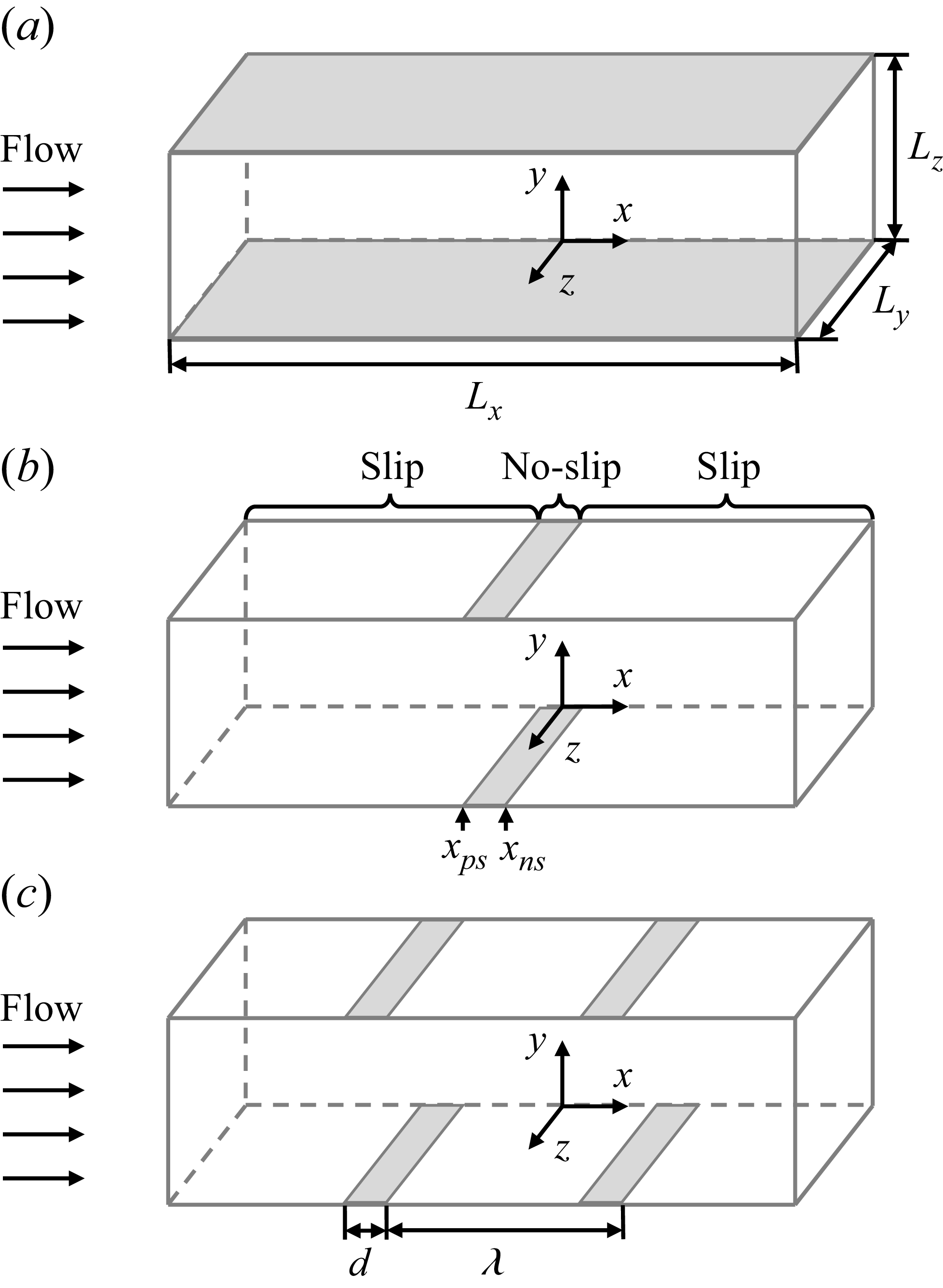
 a
 b
 n=1
 xns
 xps
 c
 n=2
 d
 λ=Lx/n
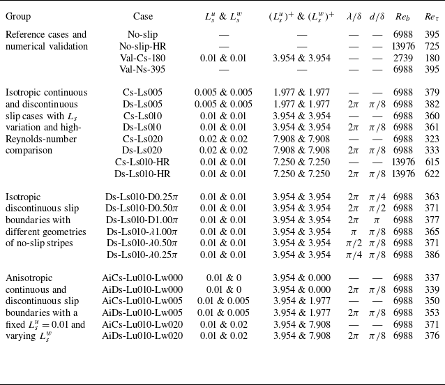
 (Lsu)+
 (Lsw)+
 ν/uτ0
 Reb=13976
 λ
 d
 λ
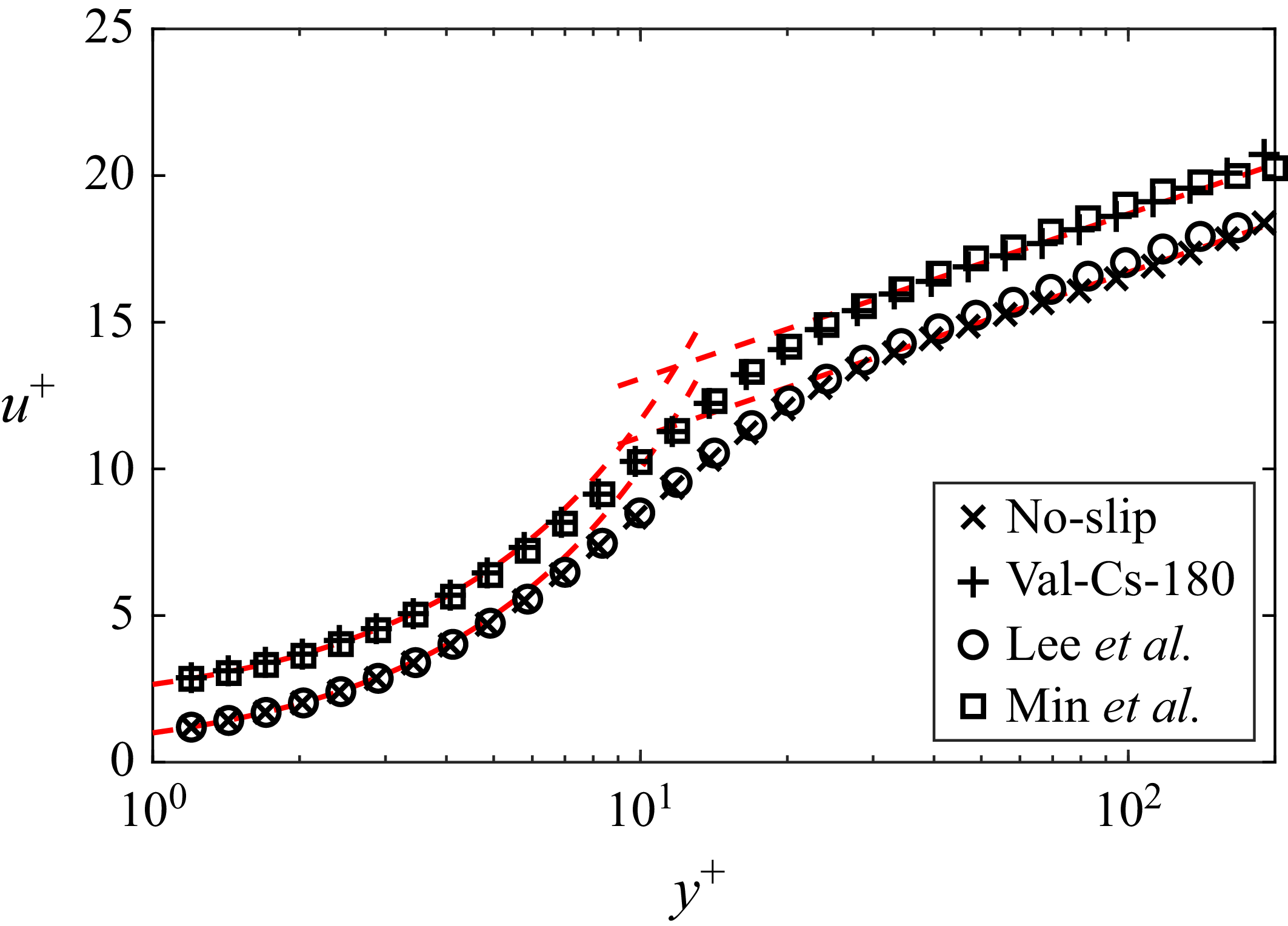
 ⟨u¯⟩+
 uτ
 y+
 ν/uτ
 Reτ=395
 Ls=0.01
 Reτ=180

 Ls
 a
 ⟨u¯⟩+
 b
 urms=⟨ui′2¯⟩0.5/uτ0
 c
 ⟨τ⟩+0
 ⟨τν⟩+0
 −⟨τR⟩+0
 d
 −⟨u~v~⟩+
 d/δ=π/8,λ/δ=2π
 Ls
 Ls

 Reτ
 a
 ⟨u¯⟩+
 b
 urms=⟨ui′2¯⟩0.5/uτ0
 c
 ⟨τ⟩+0
 ⟨τν⟩+0
 −⟨τR⟩+0
 d
 −⟨u~v~⟩+
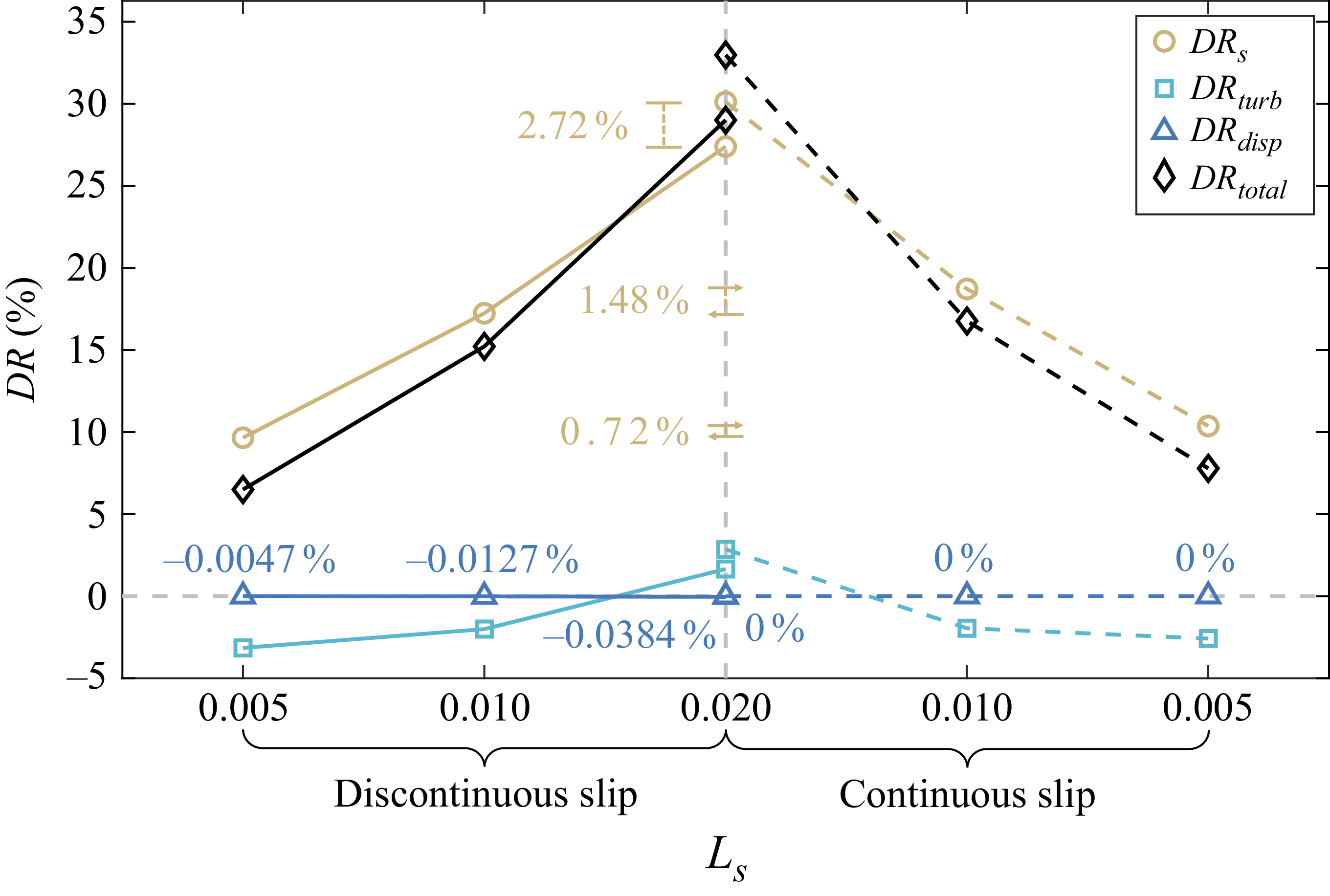
 DRtotal
 Ls
 DRtotal
 ⋄
 DRs
 ∘
 DRturb
 ◻
 DRdisp
 △
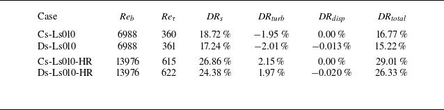
 DRtotal=DRs+DRturb+DRdisp
 Ls=0.01

 Ls=0.005
 a
 ⟨p¯⟩z+
 b
 uτ,w+0
 y+=0
 x/δ

 Q
 Q+0=0.01
 a
 Ls=0.005
 b
 Ls=0.01
 c
 Ls=0.02
 u/ub
 d
 ⟨f¯Q⟩
 e
 ⟨Q+0⋅fQ¯⟩
 f
 ⟨Q+0⋅fQ¯⟩/⟨f¯Q⟩
 Ls
 Ls

 d
 λ
 Ls=0.01
 a
 ⟨u¯⟩+−us+
 b
 urms=⟨ui′2¯⟩0.5/uτ0
 c
 ⟨τ⟩+0
 ⟨τν⟩+0
 −⟨τR⟩+0
 d
 −⟨u~v~⟩+
 d
 π
 π
 π
 λ/δ=2π
 λ
 λ
 π
 λ
 π
 λ
 π
 d/δ=π/8

 DRtotal
 d
 λ
 a
 DRtotal
 ⋄
 DRs
 ∘
 DRturb
 ◻
 DRdisp
 △
 d
 π
 π
 π
 λ
 λ
 π
 λ
 π
 λ
 π
 b
 DRs

 Q+0=0.01
 a
 Ls=0.01
 b
 d/δ=π
 λ/δ=2π
 π
 c
 d/δ=π/8
 λ/δ=π/4
 λ
 π
 u/ub
 d
 ⟨f¯Q⟩
 e
 ⟨Q+0⋅fQ¯⟩
 f
 ⟨Q+0⋅fQ¯⟩/⟨f¯Q⟩
 d
 λ
 Ls=0.01
 d
 λ/δ=2π
 λ
 d/δ=π/8
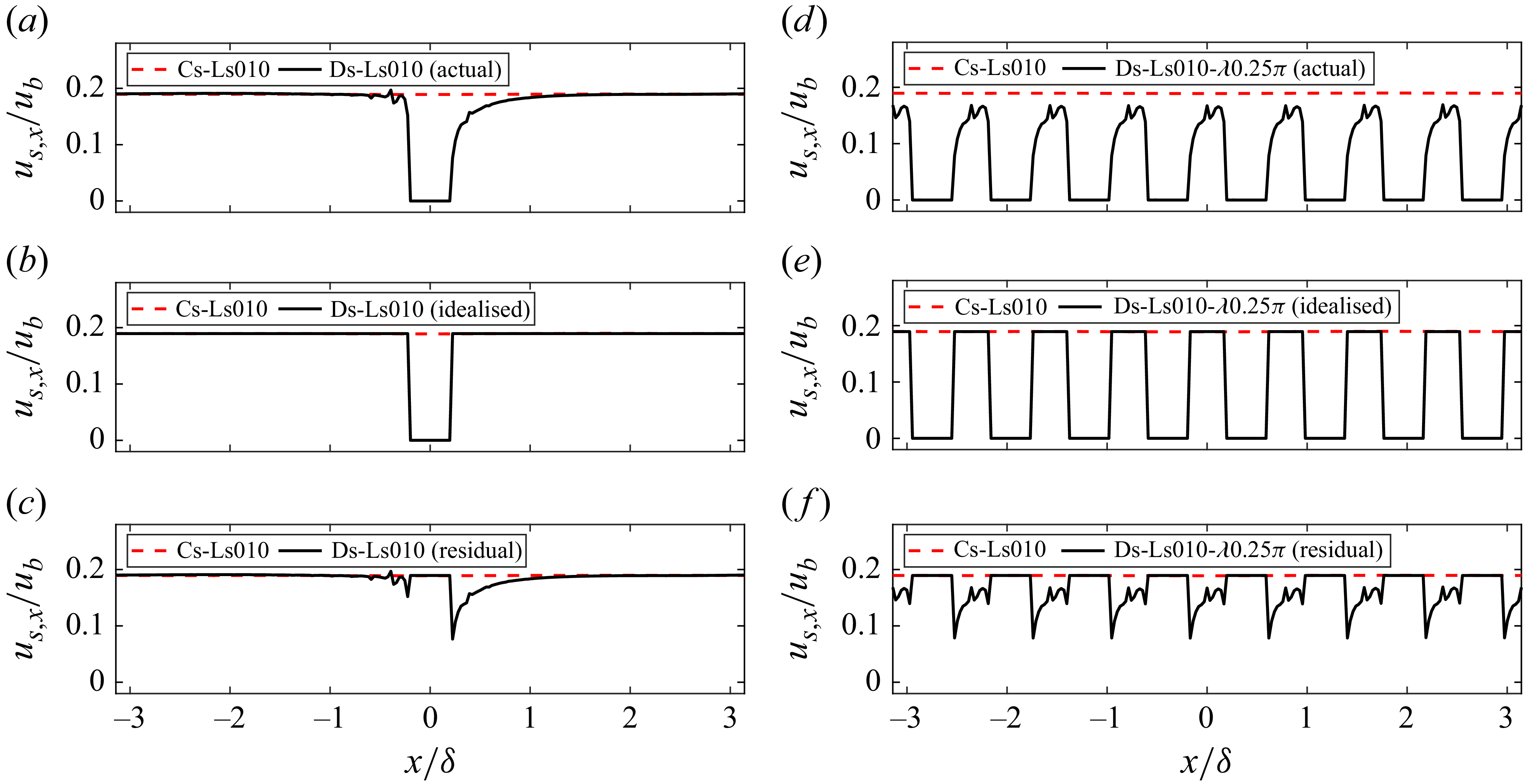
 us,x
 ub
 Ls=0.01
 a
 us,x
 b
 us,x
 c
 us,x
 λ
 π
 d
 us,x
 e
 us,x
 f
 us,x

 Lsw
 Lsu=0.01
 a
 ⟨u¯⟩+
 b
 urms=⟨ui′2¯⟩0.5/uτ0
 c
 ⟨τ⟩+0
 ⟨τν⟩+0
 −⟨τR⟩+0
 d
 −⟨u~v~⟩+
 Lsw
 Lsw
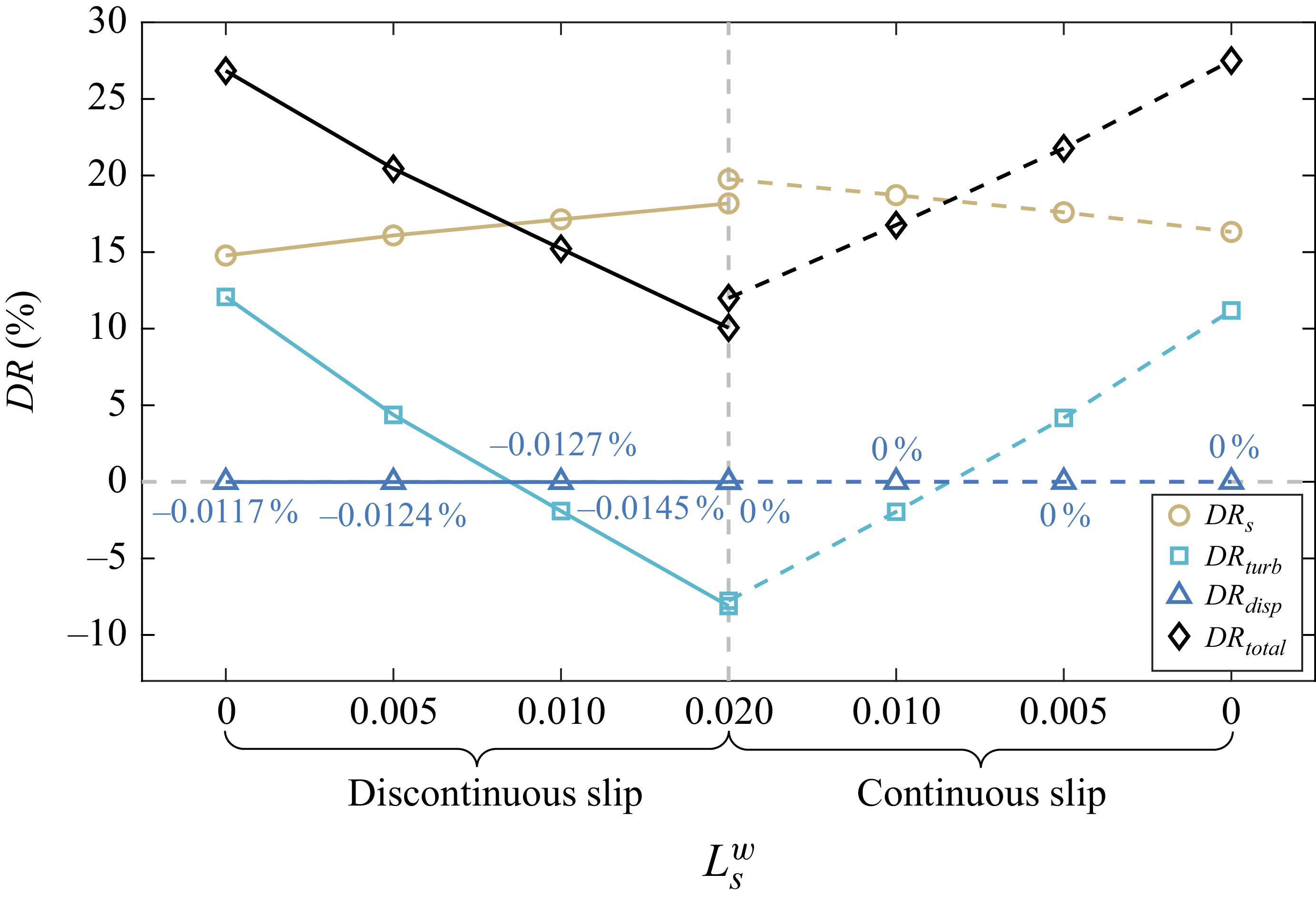
 DRtotal
 Lsw
 a
 DRtotal
 ⋄
 DRs
 ∘
 DRturb
 ◻
 DRdisp
 △

 Q+0=0.01
 Lsu=0.01
 a
 Lsw=0
 b
 Lsw=0.005
 c
 Lsw=0.02
 u/ub
 d
 ⟨f¯Q⟩
 e
 ⟨Q+0⋅fQ¯⟩
 f
 ⟨Q+0⋅fQ¯⟩/⟨f¯Q⟩
 Lsw
 Lsu=0.01

 ⟨u¯⟩z/ub
 Ls=0.01
 a
 d/δ=π/8,λ/δ=2π
 b
 π
 d/δ=π,λ/δ=2π
 c
 λ
 π
 d/δ=π/8,λ/δ=π/4
 y+0
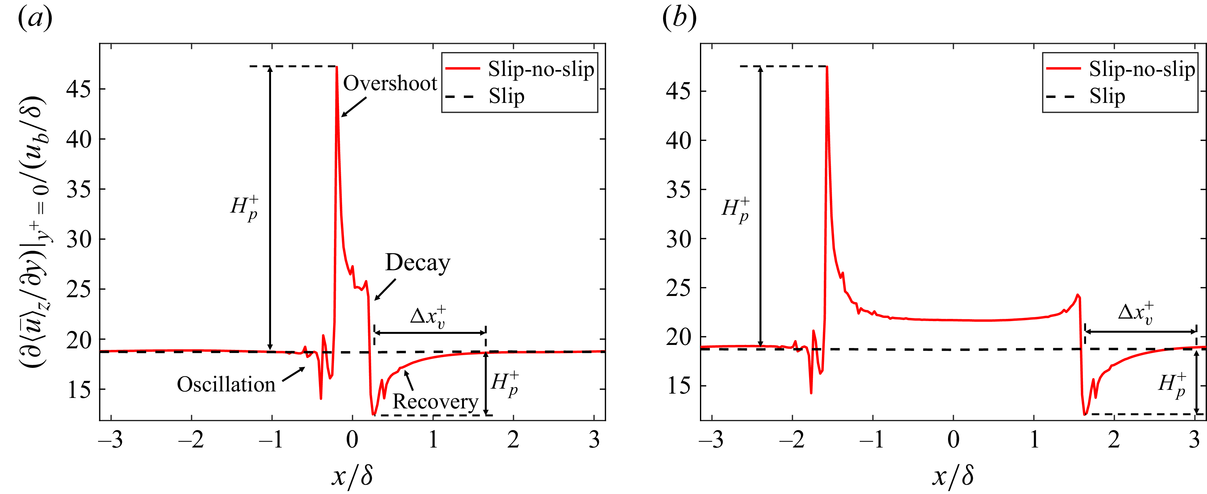
 ∂⟨u¯⟩z/∂y
 y+=0
 ub/δ
 a
 d/δ=π/8
 b
 π
 d/δ=π
 Ls=0.01
 Hp+
 Hv+
 Δxv+

 C(Φi)
 Ls=0.01
 a
 d/δ=π/8
 b
 π
 d/δ=π
 Φc
 Φp
 Φν
 Φτ
 S
 x/δ

 ⟨u¯⟩z+
 urms,z
 Δxns
 a,b
 d/δ=π/8
 c,d
 π
 d/δ=π
 ◻
 ∘
 Reb
 xns

 ⟨u¯⟩z+
 urms,z
 Δxps
 a,b
 d/δ=π/8
 c,d
 π
 d/δ=π
 ◻
 ∘
 Reb
 xps
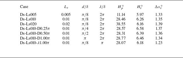
 Hp+
 Hv+
 Δxv+
 Ls
 d
 λ

 π
 Ls=0.01
 a
 Δu0+
 b
 Δul+
 ×
 Δu0+=0
 Δul+=0

 ⟨k¯⟩z+0
 x+∈[−450,450]
 y+∈[0,50]
 a
 b
 Ls=0.01
 c
 Ls=0.01

 a
 ⟨k¯⟩+0
 b
 ⟨P⟩+
 c
 ⟨ε⟩+
 d
 ⟨T⟩total+
 Ls
 Ls

 a
 ⟨k¯⟩+0
 b
 ⟨P⟩+
 c
 ⟨ε⟩+
 d
 ⟨T⟩total+
 d
 λ
 Ls=0.01
 d
 π
 π
 π
 λ/δ=2π
 d/δ=π/8
 λ/δ=2π
 λ
 λ
 π
 λ
 π
 λ
 π
 d/δ=π/8

 a
 ⟨k¯⟩+0
 b
 ⟨P⟩+
 c
 ⟨ε⟩+
 d
 ⟨T⟩total+
 Lsw
 Lsu=0.01
 Lsu=0.01
 Lsw

 ⟨u′v′¯⟩+0
 a
 Ls
 b
 d
 λ
 Ls=0.01
 d/δ=π/8,λ/δ=2π
 c
 Lsu=0.01
 Lsw
 Lsu=Lsw=0.01


