1 Introduction
Originally derived for a uniform free-surface turbulent channel flow driven by gravitational acceleration, Manning’s empirical formula (Manning Reference Manning1891) relates the time- and cross-sectional area-averaged velocity
 $V$
to the hydraulic radius (
 $R_{h}$
) and the energy grade line slope (
 $S$
) through an empirical roughness coefficient
 $n$
that only varies with surface roughness (figure 1). This roughness coefficient was proposed well before the classical pipe flow resistance experiments by Nikuradse and Colebrook in the 1930s. First presented by Gauckler (in 1867) for
 $S<0.0007$
and later by Manning (in 1891) for open channels and pipes, the formula is given in SI units as (Gauckler Reference Gauckler1867; Manning Reference Manning1891; Powell Reference Powell1960)
 $$\begin{eqnarray}\displaystyle V=\frac{Q}{A}=\frac{1}{n}R_{h}^{2/3}S^{1/2}, & & \displaystyle\end{eqnarray}$$
where
 $Q$
is the volumetric flow rate,
 $A$
is the cross-sectional area orthogonal to the flow direction,
 $R_{h}=A/P_{w}$
and
 $P_{w}$
is the wetted perimeter. Because of the large corpus of supporting data, Manning’s formula is widely used in hydrology, hydraulics, sanitary engineering, irrigation science and stream restoration (Chow Reference Chow1959). As early as 1899, it was marked as ‘one of best formulas of the day’ (Willcocks & Holt Reference Willcocks and Holt1899; Powell Reference Powell1960), and this assessment remains unchanged (Brutsaert Reference Brutsaert2005). In operational hydraulics, no equation has been advanced to displace Manning’s formula to date despite all the progress made in turbulent boundary-layer theories. Thus, derivation of Manning’s equation from theories of turbulence remained lacking until recently (Gioia & Bombardelli Reference Gioia and Bombardelli2002). Using a phenomenological theory of turbulence and scaling arguments about the dominant size of vortices responsible for much of the momentum transport near granular roughness elements of uniform size
 $r$
, Gioia & Bombardelli (Reference Gioia and Bombardelli2002) (hereafter referred to as GB02) provided a theoretical derivation of Manning’s equation and a link between the Strickler scaling, namely
 $n\sim r^{1/6}$
, and Kolmogorov’s
 $k^{-5/3}$
scaling for inertial subrange turbulence (where
 $k$
is the wavenumber).
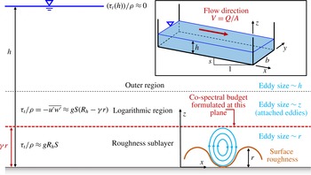
Schematic representation of turbulent flow in a rectangular channel having a width
 $b$
and a water depth
 $h$
. Flow within a very-high-Reynolds-number turbulent boundary layer over roughness elements with undulation size
 $r$
is characterized by three sublayers: (i) the roughness sublayer, where eddy sizes responsible for momentum transport generally scale with
 $r$
instead of
 $z$
(distance from boundary); (ii) an extensive logarithmic region, where eddy sizes responsible for momentum transport scale with
 $z$
(attached eddies); (iii) the outer region, where the eddy sizes tend to be large and scale with
 $h$
. The CSB is formulated near the top of the roughness sublayer at
 $z=\unicode[STIX]{x1D6FE}r$
(
 $\unicode[STIX]{x1D6FE}>1$
) just below the logarithmic region. Roughness undulations are assumed to be periodic in the
 $y$
direction and are assumed not to induce wakes or flow separation. Any secondary circulation that may form at the corners of the channel is ignored. The axes are aligned such that
 $x$
and
 $z$
are the longitudinal and vertical directions respectively.

However, several unresolved issues remain with the derivation proposed in GB02 which are incompatible with what is known about flow statistics within the roughness sublayer (hereafter referred to as RSL). These issues are to be discussed in § 2 but are summarized here to clarify the aims, scope and objectives of the present work. To begin with, GB02 assumed that eddies whose size exceeds the roughness element
 $r$
do not contribute appreciably to the vertical velocity component near roughness elements, which is not supported by theories for the RSL (Raupach, Antonia & Rajagopalan Reference Raupach, Antonia and Rajagopalan1991). Furthermore, Kolmogorov’s scaling (Kolmogorov Reference Kolmogorov1941) rarely holds in close proximity to the wall, whether it is rough or smooth (see, e.g. Poggi, Porporato & Ridolfi Reference Poggi, Porporato and Ridolfi2002; McKeon & Morrison Reference McKeon and Morrison2007), in contrast to the assumption by GB02. GB02 also employed scaling arguments to estimate the near-wall turbulent shear stress which, although plausible, were never corroborated by experiments. Last but not least, GB02 assumed that the turbulent kinetic energy dissipation rate in the vicinity of the roughness elements scales as
 $V^{3}/R_{h}$
, and that the associated similarity constant is independent of
 $r/R_{h}$
, which, as will be discussed later on, cannot be correct given what is known about the flow properties in the RSL (Raupach Reference Raupach1981; Raupach et al.
Reference Raupach, Antonia and Rajagopalan1991).
The present work addresses these issues as follows. In § 2, a brief overview of GB02 and a critical appraisal of their assumptions is provided. An approach based on a co-spectral budget (hereafter referred to as CSB) model is developed, and it is then shown that Manning’s formula can be recovered when assuming a simplified formulation for the vertical velocity spectra
 $E_{ww}(k)$
which accommodates deviations from
 $k^{-5/3}$
at low
 $k$
. This simplifying hypothesis is discussed in § 3, where a sensitivity analysis of the proposed model is performed by integrating the CSB budget equation over the entire flow domain and using more complex (and perhaps more realistic) shapes for
 $E_{ww}(k)$
. It is shown that the CSB model, besides capturing the main features of mean velocity profiles, also reproduces Nikuradse’s data on friction factors in the fully rough regime. The results also confirm that Strickler’s scaling represents a reasonable but inaccurate fit of experimental data also established by the Colebrook equation. There is no reason why it should have a ‘clean’ theoretical origin as suggested by GB02. Finally, a comparison between literature values of Manning’s coefficient and those predicted from the CSB is presented over seven decades of
 $r$
variation in § 4. The results provide novel links between Manning’s roughness coefficient, velocity–pressure interactions and the vertical velocity spectrum highlighted in the discussion and conclusion (§ 5).
2 Theory
2.1 Background
In a steady and uniform open channel flow within a rectangular section having a water depth
 $h$
and a width
 $b$
(figure 1), let
 $u$
denote the velocity component along the longitudinal direction
 $x$
and
 $w$
the velocity component in the bed-normal direction
 $z$
(positive upward). The total shear stress
 $\unicode[STIX]{x1D70F}_{0}$
uniformly distributed along
 $P_{w}=2h+b$
(i.e. grains of size
 $r$
are uniformly distributed along the bed and channel sides) can be determined from a force balance, resulting in
 $$\begin{eqnarray}\displaystyle \frac{\unicode[STIX]{x1D70F}_{0}}{\unicode[STIX]{x1D70C}}=gR_{h}S, & & \displaystyle\end{eqnarray}$$
where
 $\unicode[STIX]{x1D70C}$
is the fluid density and
 $g$
is the gravitational acceleration. In fully rough flow regimes and at some small distance from the wall,
 $\unicode[STIX]{x1D70F}_{0}$
mainly originates from turbulent shear stress contributions given as
 $$\begin{eqnarray}\displaystyle \frac{\unicode[STIX]{x1D70F}_{0}}{\unicode[STIX]{x1D70C}}=u_{\ast }^{2}\sim \max (-\overline{u^{\prime }w^{\prime }}), & & \displaystyle\end{eqnarray}$$
where
 $\overline{u^{\prime }w^{\prime }}$
is the turbulent momentum flux with a maximum in magnitude adjacent to
 $P_{w}$
, an overbar denotes time averaging,
 $u^{\prime }$
and
 $w^{\prime }$
are the turbulent longitudinal and bed-normal fluctuations from
 $u$
and
 $w$
respectively and
 $u_{\ast }$
is the shear or friction velocity corresponding to the bed stress
 $\unicode[STIX]{x1D70F}_{0}$
. A drag coefficient or friction factor given by
 $f_{d}=u_{\ast }^{2}/V^{2}$
can be inserted into (2.2) and combined with (2.1) to recover the classical Chezy formula
 $V={f_{d}}^{-1/2}\sqrt{gR_{h}S}$
derived in 1776. The term
 $C_{z}={f_{d}}^{-1/2}$
is the Chezy coefficient and was initially assumed to vary with
 $r$
only. Here,
 $f_{d}$
can be related to the well-known Darcy–Weisbach friction factor
 $f=8f_{d}$
, as discussed elsewhere (Brown Reference Brown2002). Upon equating the Chezy
 $V=C_{z}\sqrt{gR_{h}S}$
to Manning’s formula in (1.1), it becomes clear that
 $C_{z}=R_{h}^{1/6}g^{-1/2}n^{-1}$
. Dimensional considerations alone suggest that
 $C_{z}$
must vary with the ratio
 $r/R_{h}$
if
 $n$
only varies with
 $r$
, as presumed in the original work of Manning. That is,
 $C_{z}=F(r/R_{h})$
, where
 $F(.)$
is an unknown function which may be determined from incomplete similarity (i.e.
 $K_{1}(r/R_{h})^{a}+o[(r/R_{h})^{a}]$
and
 $K_{1}$
is a similarity constant). Incomplete similarity is necessary to determine the form of
 $F(.)$
because when
 $r\rightarrow 0$
,
 $C_{z}$
does not approach a constant as predicted by complete similarity (Barenblatt Reference Barenblatt1996). When
 $r$
is sufficiently small to be entirely embedded within the viscous sublayer,
 $C_{z}$
must approach its smooth-wall formulation expressed as a function of the bulk Reynolds number
 $Re=VR_{h}/\unicode[STIX]{x1D708}$
, where
 $\unicode[STIX]{x1D708}$
is the kinematic viscosity. Stated differently, incomplete similarity predicts
 $C_{z}=F(r/R_{h})+G(Re)$
, where
 $G(Re)$
encodes the smooth boundary-layer solution expressed as
 $f_{d}\sim Re^{-\unicode[STIX]{x1D6FC}}$
, with
 $\unicode[STIX]{x1D6FC}=1$
for laminar flow and
 $\unicode[STIX]{x1D6FC}=1/4$
for turbulent flows at moderate
 $Re$
(i.e. Blasuis scaling) as discussed elsewhere (McKeon, Zagarola & Smits Reference McKeon, Zagarola and Smits2005). With increasing
 $Re$
,
 $G(Re)$
is asymptotically reduced relative to
 $F(r/R_{h})$
when
 $r>0$
and
 $R_{h}\gg r$
. With such a naive argument, it becomes evident that if
 $C_{z}$
only varies with
 $r/R_{h}$
and
 $C_{z}\sim R_{h}^{1/6}n^{-1}$
, incomplete similarity must predict
 $a=-1/6$
, resulting in
 $n^{-1}\sim r^{-1/6}$
. Here,
 $a=-1/6$
is the well-known Strickler scaling at very high
 $Re$
(i.e.
 $G(Re)/F(r/R_{h})\ll 1$
). This is one of the results featured in the dimensional consideration by GB02.
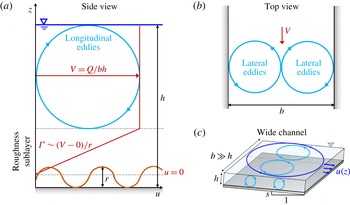
(a,b) The linkage between the local variables
 $\unicode[STIX]{x1D6E4}$
and
 $\unicode[STIX]{x1D716}$
and the bulk variables
 $V$
,
 $R_{h}$
and the roughness size
 $r$
for uniform flow in a channel with width
 $b$
and water depth
 $h$
. Above the roughness sublayer, the bulk velocity is assumed to be
 $V\sim Q/(bh)$
. Within the roughness elements, the mean velocity
 $u$
is assumed to be negligible. Hence, defining the roughness sublayer thickness to be proportional to
 $r$
results in
 $\unicode[STIX]{x1D6E4}\sim (V-0)/r$
. Because the mean flow kinetic energy is constant along
 $x$
in uniform flows, the
 $\unicode[STIX]{x1D716}$
must be dissipated by the production of turbulent eddies. The inverse time scale (
 $T_{L}^{-1}$
) of the primary eddies is
 $V/h$
for the longitudinal eddies and
 $V/(b/2)$
for the lateral eddies, as discussed elsewhere (Gioia & Bombardelli Reference Gioia and Bombardelli2002). (c) Schematic representation of a wide channel with eddies of different sizes.

2.2 Review and critical appraisal of GB02’s derivation
The salient features of the derivation of Manning’s formula in GB02 are now provided for completeness. When analysing the dominant velocity scales contributing to
 $\max (-\overline{u^{\prime }w^{\prime }})$
at the top of the roughness elements, it was assumed by GB02 that
 $u^{\prime }\sim V$
. A plausibility argument in support of this assumption is provided by Gioia and co-workers in a subsequent paper (Gioia et al.
Reference Gioia, Guttenberg, Goldenfeld and Chakraborty2010) and goes as follows. At any elevation above the bed, the turbulent shear stress can be thought of as a product between the momentum contrast (i.e.
 $\unicode[STIX]{x1D70C}s\text{d}\overline{u}/\text{d}z$
, where
 $s$
is the characteristic scale over which velocity gradients occur) and the rate of momentum transfer (i.e.
 $w_{s}$
, which indicates the velocity scale of an eddy of size
 $s$
), and hence
 $\unicode[STIX]{x1D70F}(z)=-\unicode[STIX]{x1D70C}\overline{u^{\prime }w^{\prime }}\sim \unicode[STIX]{x1D70C}(s\text{d}\overline{u}/\text{d}z)w_{s}$
. At the roughness tops,
 $s\sim r$
and
 $\text{d}\overline{u}/\text{d}z\sim (V-0)/r$
, resulting in
 $u^{\prime }\sim V$
, as shown in figure 2. With regards to
 $w^{\prime }$
, GB02 assumed that eddies of size
 $s\sim r$
contribute appreciably to the turnover velocity acting on
 $\text{d}u/\text{d}z$
, so that
 $w^{\prime }\sim w_{s}\sim w_{r}$
. Here,
 $w_{r}$
is associated with eddies of size
 $r$
which ‘fill’ the roughness elements, as shown in figure 1. To infer its magnitude, the Kolmogorov scaling for the inertial subrange was assumed so that
 $|w_{r}|\sim (\unicode[STIX]{x1D716}r)^{1/3}$
, and the concomitant turbulent momentum flux becomes
 $$\begin{eqnarray}\displaystyle gR_{h}S=\max (-\overline{u^{\prime }w^{\prime }})\sim Vw_{r}\sim V(\unicode[STIX]{x1D716}r)^{1/3}, & & \displaystyle\end{eqnarray}$$
where
 $\unicode[STIX]{x1D716}$
is the mean turbulent kinetic energy dissipation rate to be determined. In principle,
 $\unicode[STIX]{x1D716}$
must be interpreted as the dissipation rate just above the roughness elements. However, GB02 argued that such a local
 $\unicode[STIX]{x1D716}(z=r)$
and bulk dissipation rate (
 $\unicode[STIX]{x1D716}_{b}$
) are proportional, thereby allowing them to assume
 $\unicode[STIX]{x1D716}\sim \unicode[STIX]{x1D716}_{b}$
. To infer this
 $\unicode[STIX]{x1D716}_{b}$
, it is noted that the mean flow kinetic energy is unaltered spatially by frictional losses in a steady uniform flow (by definition). It follows that the total energy losses are due to turbulence and scale with
 $V^{2}$
, leading to
 $\unicode[STIX]{x1D716}_{b}\sim V^{2}/T_{L}$
. Here,
 $T_{L}$
reflects the lifetime of turbulent eddies dissipating the work done in moving the fluid against wall and bed friction (or wetted perimeter). As in GB02, figure 2 shows that the eddy frequency
 $1/T_{L}$
must include contributions from longitudinal and lateral eddies whose inverse lifetimes scale as
 $V/h$
and
 $V/(b/2)$
. It directly follows that
 $T_{L}^{-1}=V/R_{h}$
, leading to
 $$\begin{eqnarray}\displaystyle \unicode[STIX]{x1D716}\sim \unicode[STIX]{x1D716}_{b}\sim \frac{V^{3}}{R_{h}}, & & \displaystyle\end{eqnarray}$$
so that
 $w_{r}\sim (r/R_{h})^{1/3}V$
. Combining (2.3) and (2.4), Manning’s formula comprehensive of Strickler’s scaling was recovered by GB02 as
 $$\begin{eqnarray}\displaystyle V\sim \left(\frac{r}{R_{h}}\right)^{-1/6}\sqrt{R_{h}gS}. & & \displaystyle\end{eqnarray}$$
The derivation proposed by GB02 contains some implicit assumptions which are now discussed. The first (labelled as assumption A1) deals with the estimation of
 $u^{\prime }\sim V$
, or implicitly
 $\unicode[STIX]{x1D6E4}(z)=\text{d}u(z)/\text{d}z\sim V/r$
, while the second (assumption A2) deals with the estimation of
 $\unicode[STIX]{x1D716}(z)$
near the top of the roughness elements as a function of bulk variables. With regards to assumption A1, figure 2 provides a plausibility argument that in the vicinity of the roughness elements,
 $\unicode[STIX]{x1D6E4}$
may be estimated from
 $$\begin{eqnarray}\displaystyle |\unicode[STIX]{x1D6E4}|\sim \frac{V-0}{r}, & & \displaystyle\end{eqnarray}$$
when
 $u=0$
within the roughness elements and the thickness of the roughness sublayer scales with
 $r$
. More significant in GB02 is that the proportionality constant
 $\unicode[STIX]{x1D6FC}_{1}$
linking
 $\unicode[STIX]{x1D6E4}$
to
 $V/r$
(i.e.
 $\unicode[STIX]{x1D6E4}=\unicode[STIX]{x1D6FC}_{1}V/r$
) is assumed to be independent of
 $r/R_{h}$
. The implicit assumption about the independence of
 $\unicode[STIX]{x1D6FC}_{1}$
from
 $r/R_{h}$
, at the very least, is questionable in the RSL.
To illustrate, let the plane of analysis be vertically displaced from the roughness tops to an elevation right at the beginning of the logarithmic layer (figure 1), where it is possible to exploit the known scaling for energy dissipation and the mean velocity gradient. This is one of the novelties introduced by the CSB approach explained later, but it is also used here to critically analyse the GB02 approach. This switch in point of analysis is small and is typically a linear function of
 $r$
. Detailed experiments on flow over granular roughness elements reported a log region commencing at approximately
 $z=\unicode[STIX]{x1D6FE}r$
independent of
 $R_{h}$
with
 $\unicode[STIX]{x1D6FE}=1.6$
(Manes, Pokrajac & McEwan Reference Manes, Pokrajac and McEwan2007). Therefore, the scaling for both the mean velocity gradient and the dissipation rate proposed by GB02 should not be affected by this switch in the plane of analysis provided that
 $r/R_{h}$
is small. At this location (i.e.
 $z\sim r$
), the local mean velocity gradient can be assumed to scale as
 $\text{d}\overline{u}/\text{d}z\sim u_{\ast }/r$
. This observation, when combined with (2.6), implies that
 $\unicode[STIX]{x1D6FC}_{1}$
must scale as the square root of the Darcy–Weisbach friction factor (i.e.
 $\unicode[STIX]{x1D6FC}_{1}\sim f_{d}^{1/2}$
), which notoriously depends on the relative roughness
 $r/R_{h}$
in fully rough turbulent flows.
With regards to assumption A2, there are two separate issues to be discussed. The first issue is whether the bulk dissipation
 $\unicode[STIX]{x1D716}_{b}$
itself is correct when assuming it to be independent from
 $r/R_{h}$
and only proportional to the bulk variables
 $V$
and
 $R_{h}$
, as shown by (2.4). The second issue is whether
 $\unicode[STIX]{x1D716}_{b}$
represents the local
 $\unicode[STIX]{x1D716}(z\approx r)$
near the roughness top. The first issue is inconsistent with simple thermodynamic considerations applied to the bulk flow irrespective of whether the local
 $\unicode[STIX]{x1D716}$
at the top of the roughness elements can be equated or proportional to
 $\unicode[STIX]{x1D716}_{b}$
as in GB02 (i.e. the second issue). To illustrate, the work
 $W_{e}$
required to move a fluid mass over a distance
 $L$
is
 $W_{e}=\unicode[STIX]{x1D70F}_{0}AL=\unicode[STIX]{x1D70F}_{0}$


 $=A\times L$
the fluid volume. Upon inserting (2.1), the work per unit mass to move the fluid is W
e
′
= W
e
/(𝜌

 $W_{e}^{\prime }=f_{d}V^{2}$
. The bulk turbulence kinetic energy (TKE) dissipation rate is the change in work during a turnover time, resulting in
 $\unicode[STIX]{x1D716}_{b}\sim W_{e}^{\prime }/T_{L}\sim f_{d}V^{3}/R_{h}$
. While the scaling in (2.4) is actually recovered (i.e.
 $\unicode[STIX]{x1D716}_{b}\sim V^{3}/R_{h}$
), it is evident that
 $\unicode[STIX]{x1D716}_{b}$
cannot be independent of
 $r/R_{h}$
because
 $f_{d}$
varies with
 $r/R_{h}$
, as already hinted at from the incomplete similarity argument in the previous section. The same result can be obtained even more rigorously by integrating the TKE balance equation across the whole flow domain presented elsewhere (Abe & Antonia Reference Abe and Antonia2016).
With regards to the second issue, we assume that the local dissipation at the roughness tops can be quantified by means of bulk variables as follows:
 $$\begin{eqnarray}\displaystyle \unicode[STIX]{x1D716}(z=r)=\frac{\unicode[STIX]{x1D6FC}_{2}^{3}V^{3}}{R_{h}}, & & \displaystyle\end{eqnarray}$$
where
 $\unicode[STIX]{x1D6FC}_{2}$
is an ad hoc scaling function which allows for the transition from local to bulk variables at a given
 $z$
and
 $r/R_{h}$
. Now, in the RSL just below the log layer, the local dissipation rate can be computed as
 $\unicode[STIX]{x1D716}(z=r)=-\overline{u^{\prime }w^{\prime }}\text{d}u/\text{d}z\sim (u_{\ast }^{3})/r$
because
 $\text{d}u/\text{d}z\sim u_{\ast }/r$
. Inserting this result into (2.7) implies that
 $\unicode[STIX]{x1D6FC}_{2}$
must scale as
 $\unicode[STIX]{x1D6FC}_{2}\sim (R_{h}/r)^{1/3}f_{d}^{1/2}$
. Repeating the derivation of GB02 while accounting for the correct scaling functions for the mean velocity gradient and the local dissipation rate, one obtains
 $$\begin{eqnarray}\displaystyle gR_{h}S\sim V(\unicode[STIX]{x1D716}r)^{1/3}\sim \unicode[STIX]{x1D6FC}_{1}\unicode[STIX]{x1D6FC}_{2}V^{2}\left(\frac{r}{R_{h}}\right)^{1/3}, & & \displaystyle\end{eqnarray}$$
and ultimately
 $$\begin{eqnarray}\displaystyle V\sim (\unicode[STIX]{x1D6FC}_{1}\unicode[STIX]{x1D6FC}_{2})^{-1/2}\left(\frac{r}{R_{h}}\right)^{-1/6}\sqrt{R_{h}gS}. & & \displaystyle\end{eqnarray}$$
Strickler’s scaling in (2.9) is recovered only if the product
 $\unicode[STIX]{x1D6FC}_{1}\unicode[STIX]{x1D6FC}_{2}$
is constant. From the previous analysis, it turns out that
 $\unicode[STIX]{x1D6FC}_{1}\unicode[STIX]{x1D6FC}_{2}\sim (r/R_{h})^{-1/3}f_{d}$
, which becomes constant only if the friction factor
 $f_{d}$
follows the Strickler scaling (i.e.
 $f_{d}\sim (r/R_{h})^{1/3}$
). This finding leads to a circular argument. Manning’s formula and the Strickler scaling can only be recovered if
 $\unicode[STIX]{x1D6FC}_{1}\unicode[STIX]{x1D6FC}_{2}$
is constant independent of
 $r/R_{h}$
, but
 $\unicode[STIX]{x1D6FC}_{1}\unicode[STIX]{x1D6FC}_{2}$
is independent of
 $r/R_{h}$
only when the Strickler scaling applies. These are the main reasons why the derivation of Manning’s formula is re-examined using an alternative approach based on the CSB model which eliminates the need to a priori link local to global variables.
2.3 Co-spectral budget model
The focus here is on wide channels, so that
 $R_{h}\approx h$
, although many of the results derived next hold when replacing
 $h$
with
 $R_{h}$
. The momentum turbulent flux at any height
 $z>r$
from the surface (or boundary) can be linked to eddy sizes characterized by wavenumber
 $k$
through the normalizing property of the co-spectrum, given by
 $$\begin{eqnarray}\displaystyle \overline{u^{\prime }w^{\prime }}=-\int _{0}^{\infty }F_{wu}(k)\,\text{d}k, & & \displaystyle\end{eqnarray}$$
where
 $k$
corresponds to an inverse eddy size,
 $F_{wu}(k)$
is the co-spectrum between
 $u^{\prime }$
and
 $w^{\prime }$
, and where
 $-\overline{u^{\prime }w^{\prime }}(z)\approx (ghS)(1-z/h)$
, as expected in open channel flows for
 $z>r$
. The
 $F_{wu}(k)$
can now be modelled through a budget formulated in the RSL above the roughness elements at
 $z=\unicode[STIX]{x1D6FE}r$
with
 $\unicode[STIX]{x1D6FE}>1$
but below the logarithmic region characterizing
 $\overline{u}(z)$
, as shown in figure 1. As already discussed, this region defines the thickness of the RSL for momentum transport, which for granular roughness results in
 $\unicode[STIX]{x1D6FE}\approx 1.6$
(Manes et al.
Reference Manes, Pokrajac and McEwan2007). It is further assumed that
 $\unicode[STIX]{x1D6FE}r/h\ll 1$
, so that at
 $z=\unicode[STIX]{x1D6FE}r$
,
 $-\overline{u^{\prime }w^{\prime }}(z)\approx (ghS)\approx u_{\ast }^{2}$
. This budget is given by (Panchev Reference Panchev1971; Katul et al.
Reference Katul, Porporato, Manes and Meneveau2013; Katul & Manes Reference Katul and Manes2014)
 $$\begin{eqnarray}\displaystyle \frac{\unicode[STIX]{x2202}F_{wu}(k)}{\unicode[STIX]{x2202}t}+2\unicode[STIX]{x1D708}k^{2}F_{wu}(k)=G(k), & & \displaystyle\end{eqnarray}$$
where
 $$\begin{eqnarray}\displaystyle G(k)=P_{wu}(k)+T_{wu}(k)+\unicode[STIX]{x1D70B}(k) & & \displaystyle\end{eqnarray}$$
and
 $P_{wu}(K)=\unicode[STIX]{x1D6E4}E_{ww}(k)$
is the covariance (or turbulent stress) production term,
 $E_{ww}(k)$
is the turbulent energy spectrum of the vertical velocity,
 $\unicode[STIX]{x1D6E4}$
is now interpreted as a local mean velocity gradient across the plane where the CSB is being formulated (i.e.
 $z=\unicode[STIX]{x1D6FE}r$
),
 $T_{wu}(k)$
is the co-spectral flux-transfer term and
 $\unicode[STIX]{x1D70B}(k)$
is the velocity–pressure interaction term, which acts to decorrelate
 $u^{\prime }$
and
 $w^{\prime }$
(Pope Reference Pope2000). If a Rotta model is further invoked for
 $\unicode[STIX]{x1D70B}(K)$
but adjusted for the isotropization of the production effect, then (Rotta Reference Rotta1962; Choi & Lumley Reference Choi and Lumley2000)
 $$\begin{eqnarray}\displaystyle \unicode[STIX]{x1D70B}(k)=-C_{R}\frac{F_{wu}(k)}{\unicode[STIX]{x1D70F}_{r}(k)}-C_{I}P_{wu}(k), & & \displaystyle\end{eqnarray}$$
where
 $\unicode[STIX]{x1D70F}_{r}(k)=\unicode[STIX]{x1D716}^{-1/3}k^{-2/3}$
is a wavenumber-dependent relaxation time scale (Onsager Reference Onsager1949; Corrsin Reference Corrsin1964; Bos et al.
Reference Bos, Touil, Shao and Bertogli2004), assumed to vary only with
 $k$
and local
 $\unicode[STIX]{x1D716}$
,
 $C_{R}\approx 1.8$
and
 $C_{I}=3/5$
are the Rotta and isotropization of the production constants (Launder, Reece & Rodi Reference Launder, Reece and Rodi1975; Pope Reference Pope2000). The
 $C_{I}=3/5$
was earlier predicted from rapid distortion theory, as discussed by Pope (Reference Pope2000). Accounting for a slow part (i.e.
 $-C_{R}F_{wu}(k)/\unicode[STIX]{x1D70F}_{r}(k)$
) and a fast part (i.e.
 $C_{I}P_{wu}(k)$
) appears to be sufficient to capture
 $\unicode[STIX]{x1D70B}(k)$
in many geophysical applications such as the atmospheric boundary layer (Mellor & Yamada Reference Mellor and Yamada1982). To what extent such a representation can be extrapolated to the cross-over from the RSL to the log region may be a subject of some debate given the possible large strain rate in this layer (Choi & Lumley Reference Choi and Lumley2000). Nonlinear corrections to
 $\unicode[STIX]{x1D70B}(k)$
that satisfy realizability conditions (Schumann Reference Schumann1977) can be derived with the aid of the Cayley–Hamilton theorem using symmetry group rotations and shear deformation scale, as extensively discussed elsewhere (Pope Reference Pope1975; Lumley Reference Lumley1978; Sarkar & Speziale Reference Sarkar and Speziale1990; Taulbee Reference Taulbee1992; Gatski & Speziale Reference Gatski and Speziale1993; Chung & Kim Reference Chung and Kim1995; Shih, Zhu & Lumley Reference Shih, Zhu and Lumley1995; Girimaji Reference Girimaji1996; Johansson & Wallin Reference Johansson and Wallin1996; Jongen & Gatski Reference Jongen and Gatski1998; Rung, Thiele & Fu Reference Rung, Thiele and Fu1998; Choi & Lumley Reference Choi and Lumley2000; Gatski & Jongen Reference Gatski and Jongen2000; Pope Reference Pope2000; Jacob et al.
Reference Jacob, Biferale, Iuso and Casciola2004, Reference Jacob, Casciola, Talamelli and Alfredsson2008; Schmitt Reference Schmitt2007), and are beyond the scope here. In general, such corrections are significant when the mean advection–distortion time scale appears to be comparable to the eddy relaxation time scale, the mean flow rotation is large or when the eddy relaxation time scales are comparable to or larger than the shear deformation scale. A recent study (McColl et al.
Reference McColl, Katul, Gentine and Entekhabi2016) directly evaluated (2.13) in its spectral form using high-Reynolds-number direct numerical simulations (DNS) for a smooth boundary layer. The evaluation suggested reasonable agreement in the logarithmic and upper portion of the buffer layer (where turbulent stresses dominate the total stress), but deviations in the middle and lower portions of the buffer layers were noted. These deviations were shown to originate from wall-blocking effects instead of higher-order corrections to the rapid component of
 $\unicode[STIX]{x1D70B}(k)$
. Given the uniform nature of the flow and the assumed high Reynolds number in the RSL here (i.e.
 $\unicode[STIX]{x1D70F}_{0}=\unicode[STIX]{x1D70C}u_{\ast }^{2}$
at
 $z=\unicode[STIX]{x1D6FE}r$
), such nonlinear corrections to
 $\unicode[STIX]{x1D70B}(k)$
may be secondary except for small
 $k$
.
Assuming stationary conditions, and upon further ignoring
 $T_{wu}(K)$
and the viscous term momentarily (their effects have been separately explored and are not shown here), this budget equation, hereafter referred to as the equilibrium state, reduces to a balance between production and pressure–velocity decorrelation (i.e. destruction) terms, leading to
 $$\begin{eqnarray}\displaystyle F_{wu}(k)=\frac{1}{A_{\unicode[STIX]{x1D70B}}}\unicode[STIX]{x1D6E4}\unicode[STIX]{x1D716}^{-1/3}E_{ww}(k)k^{-2/3}, & & \displaystyle\end{eqnarray}$$
where
 $A_{\unicode[STIX]{x1D70B}}=C_{R}/(1-C_{I})\approx 4.5$
. Equations (2.13) and (2.14) neglect the wall-blocking component for the pressure–strain correlation parametrization. The implications of such an assumption were further investigated and appeared to be minor (not shown). Combining (2.10) and (2.14), the CSB at
 $z=\unicode[STIX]{x1D6FE}r$
can be re-arranged as
 $$\begin{eqnarray}\displaystyle |\unicode[STIX]{x1D6E4}|\unicode[STIX]{x1D716}^{-1/3}=A_{\unicode[STIX]{x1D70B}}\frac{-\overline{u^{\prime }w^{\prime }}}{I_{k}},\quad I_{k}=\int _{0}^{\infty }k^{-2/3}E_{ww}(k)\,\text{d}k. & & \displaystyle\end{eqnarray}$$
Interestingly, equation (2.15) can be formulated as
 $\overline{u^{\prime }w^{\prime }}=-\unicode[STIX]{x1D707}_{t}\unicode[STIX]{x1D6E4}$
, where
 $\unicode[STIX]{x1D707}_{t}=\unicode[STIX]{x1D716}^{-1/3}A_{\unicode[STIX]{x1D70B}}^{-1}I_{k}$
may be interpreted as an effective nonlinear eddy viscosity dictated by the shape of
 $k^{-2/3}E_{ww}(k)$
and the local
 $\unicode[STIX]{x1D716}(z)$
, known to vary with
 $\unicode[STIX]{x1D6E4}$
in the RSL. When the TKE budget is reduced to
 $\unicode[STIX]{x1D716}(z)=-\overline{u^{\prime }w^{\prime }}\unicode[STIX]{x1D6E4}$
,
 $\unicode[STIX]{x1D707}_{t}$
varies with
 $\unicode[STIX]{x1D6E4}$
, rendering
 $\unicode[STIX]{x1D707}_{t}$
analogous to a non-Newtonian eddy viscosity.
To evaluate
 $I_{k}$
, assumptions about the shape of
 $E_{ww}(k)$
are now required for the RSL. At
 $z=\unicode[STIX]{x1D6FE}r$
, just below the logarithmic region,
 $E_{ww}(k)$
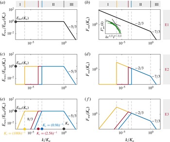
can be reasonably described by the regimes shown in figure 3. The first regime (I) is associated with low-wavenumber contributions and is delineated by
 $k\in [0,K_{c}]$
, where
 $K_{c}$
is a wavenumber commensurate with
 $R_{h}^{-1}$
or
 $h^{-1}$
. The second regime (II) is defined for
 $k\in [K_{c},K_{a}]$
, where
 $K_{a}$
is a wavenumber associated with the roughness size
 $r$
when
 $z\leqslant \unicode[STIX]{x1D6FE}r$
. The third regime (III) is delineated by
 $k>K_{a}$
, where the classical inertial subrange exists (Kolmogorov Reference Kolmogorov1941; Frisch Reference Frisch1995). The presence of regimes (II) and (III) has been confirmed by a number of field and laboratory experiments collected in the RSL above tall forested canopies (Katul et al.
Reference Katul, Geron, Hsieh, Vidakovic and Guenther1998) and in laboratory flume studies (Poggi et al.
Reference Poggi, Porporato, Ridolfi, Albertson and Katul2004). Further support for this shift in the spectral regime at
 $K_{a}\sim (z)^{-1}$
is provided by a number of recent experiments described elsewhere (Kunkel & Marusic Reference Kunkel and Marusic2006; Nickels et al.
Reference Nickels, Marusic, Hafez, Hutchins and Chong2007; Zhao & Smits Reference Zhao and Smits2007; Manes, Poggi & Ridolfi Reference Manes, Poggi and Ridolfi2011). A fourth regime also exists and is related to viscous corrections to the inertial subrange commonly formulated as an exponential cutoff (Pope Reference Pope2000) which becomes significant as
 $k$
becomes sufficiently large (i.e.
 $k\sim 1/\unicode[STIX]{x1D702}$
, where
 $\unicode[STIX]{x1D702}$
is known as the Kolmogorov microscale). However, distortions to the overall energy content (i.e.
 $\int _{0}^{\infty }E_{ww}(k)\,\text{d}k$
) and turbulent stress (i.e.
 $\int _{0}^{\infty }F_{uw}(k)\,\text{d}k$
) arising from this fourth regime vis-a-vis simply extending the inertial subrange indefinitely for
 $k>K_{a}$
are minor provided that the CSB is formulated sufficiently above the roughness elements but still below the logarithmic region, and the Reynolds number is sufficiently large to allow for large-scale separation between
 $r$
and
 $\unicode[STIX]{x1D702}$
. Moreover, bottleneck effects in
 $E_{ww}(k)$
at the cross-over from inertial to viscous range are also neglected here (Katul et al.
Reference Katul, Manes, Porporato, Bou-Zeid and Chamecki2015).
(a,c,e) Schemes of the idealized vertical velocity spectra (E1, E2 and E3) assumed in the numerical experiments. The co-spectrum
 $F_{wu}(k)$
computed in the roughness sublayer at
 $z=\unicode[STIX]{x1D6FE}r$
is also shown for each case (b,d,f). Different break points
 $K_{c}$
for cases E2 and E3 are also illustrated (c–f). The inset in (b) shows the measured shear-stress co-spectra
 $F_{uw}^{\ast }=-F_{uw}(k)/(\unicode[STIX]{x1D716}^{3}\unicode[STIX]{x1D6E4}^{-5})^{1/2}$
(original data from Saddoughi & Veeravalli (Reference Saddoughi and Veeravalli1994), digitized from Pope (Reference Pope2000)).

Integrating
 $E_{ww}(k)$
and
 $F_{uw}(k)$
to
 $k\rightarrow \infty$
is akin to assuming
 $\unicode[STIX]{x1D702}/r\sim {Re_{\ast }}^{-3/4}\rightarrow 0$
, where
 $Re_{\ast }=u_{\ast }r/\unicode[STIX]{x1D708}$
defines a roughness Reynolds number. For
 $n$
or
 $f_{d}$
to achieve independence of
 $Re_{\ast }$
,
 $Re_{\ast }$
itself must be very large but is generally finite. Upon ignoring viscous corrections and assuming that
 $Re_{\ast }$
is sufficiently large so that
 $\unicode[STIX]{x1D702}/r\ll 1$
, the idealized
 $E_{ww}(k)$
shown in figure 3 can be expressed as
 $$\begin{eqnarray}\displaystyle E_{ww}(k)=\left\{\begin{array}{@{}ll@{}}E_{kol}(K_{a})K_{c}^{-p}k^{p} & \text{if }0\leqslant k\leqslant K_{c},\\ E_{kol}(K_{a}) & \text{if }K_{c}\leqslant k\leqslant K_{a},\\ E_{kol}(k) & \text{if }k>K_{a},\end{array}\right. & & \displaystyle\end{eqnarray}$$
where
 $E_{kol}(k)=C_{o}\unicode[STIX]{x1D716}^{2/3}k^{-5/3}$
is the Kolmogorov spectrum (Kolmogorov Reference Kolmogorov1941; Frisch Reference Frisch1995),
 $C_{o}=(24/55)C_{k}^{\prime }$
is the Kolmogorov constant for the vertical velocity component and
 $C_{k}^{\prime }=1.5$
(Pope Reference Pope2000). When
 $E_{ww}(k)=E_{kol}$
,
 $F_{wu}(k)\sim \unicode[STIX]{x1D6E4}\unicode[STIX]{x1D716}^{1/3}k^{-7/3}$
, consistent with other co-spectral theories (Lumley Reference Lumley1967) and measurements (see the inset in figure 3
b, data from Saddoughi & Veeravalli (Reference Saddoughi and Veeravalli1994)) within the inertial subrange reviewed elsewhere (Katul et al.
Reference Katul, Porporato, Manes and Meneveau2013). When
 $E_{ww}(k)\approx k^{0}$
for low wavenumbers at the cross-over from inertial to larger scales as shown in figure 3, the co-spectrum scales as
 $F_{wu}(k)\approx k^{-2/3}$
when
 $\unicode[STIX]{x1D70F}_{r}(k)=\unicode[STIX]{x1D716}^{-1/3}k^{-2/3}$
. Wind tunnel experiments at very high Reynolds number in the logarithmic region indicate a co-spectral scaling between 0 and
 $-2/3$
(Saddoughi & Veeravalli Reference Saddoughi and Veeravalli1994; Pope Reference Pope2000) for values of
 $k$
smaller than those associated with the inertial subrange (see the inset in figure 3
b), but these wind tunnel experiments do not span
 $kh<1$
. Furthermore, these experiments report 1-D spectra along
 $x$
which may be distorted by the use of Taylor’s frozen turbulence hypothesis needed to convert time to wavenumbers at small
 $k$
as well as potential aliasing effects (Tennekes & Lumley Reference Tennekes and Lumley1972). This shortcoming requires further assumptions about the precise shape of
 $E_{ww}(k)$
in the very-low-wavenumber regime. Assuming a linear increase for low
 $k$
(as illustrated in figure 3, case E3), equation (2.15) becomes
 $$\begin{eqnarray}\displaystyle |\unicode[STIX]{x1D6E4}|\unicode[STIX]{x1D716}^{-1/3}=\frac{A_{\unicode[STIX]{x1D70B}}\unicode[STIX]{x1D70F}/\unicode[STIX]{x1D70C}}{\displaystyle \frac{E_{kol}(K_{a})}{K_{c}^{p}}\int _{0}^{K_{c}}k^{p}k^{-2/3}\,\text{d}k+E_{kol}(K_{a})\int _{K_{c}}^{K_{a}}k^{-2/3}\,\text{d}k+\int _{K_{a}}^{\infty }k^{-2/3}E_{kol}(k)\,\text{d}k}. & & \displaystyle \nonumber\\ \displaystyle & & \displaystyle\end{eqnarray}$$
As a first approximation, the scaling for
 $k\in [0,K_{c}]$
may be described by
 $p\sim 8/3$
(i.e. close to the von Kármán spectrum where
 $p=17/6$
). This choice is consistent with the scaling
 $p\approx 2$
suggested by Pope (Reference Pope2000), but no data exist to support it. Hence, an alternative is also explored here to assess the sensitivity of Manning’s formula to the choice of
 $p$
and
 $K_{a}$
. A constant value (i.e.
 $p=0$
and
 $K_{c}=0$
) of the energy spectrum
 $E_{ww}(k)\approx E_{kol}(K_{a})$
for low wavenumbers
 $k\in [0,K_{a}]$
(see case E1 in figure 3) to ‘boost’ the low-wavenumber eddies for
 $E_{ww}(k)$
will be considered. Using this simplified description of
 $E_{ww}(k)$
and recalling that at
 $z=\unicode[STIX]{x1D6FE}r$
,
 $\unicode[STIX]{x1D70F}/\unicode[STIX]{x1D70C}=\unicode[STIX]{x1D70F}_{0}/\unicode[STIX]{x1D70C}=ghS$
, equation (2.17) can be rewritten as
 $$\begin{eqnarray}\displaystyle |\unicode[STIX]{x1D6E4}|\unicode[STIX]{x1D716}^{-1/3}=\frac{A_{\unicode[STIX]{x1D70B}}ghS}{E_{kol}(K_{a})\displaystyle \int _{0}^{K_{a}}k^{-2/3}\,\text{d}k+\int _{K_{a}}^{\infty }k^{-2/3}E_{kol}(k)\,\text{d}k}. & & \displaystyle\end{eqnarray}$$
Upon simplifying,
 $$\begin{eqnarray}\displaystyle |\unicode[STIX]{x1D6E4}|\unicode[STIX]{x1D716}^{1/3}=\frac{4A_{\unicode[STIX]{x1D70B}}}{15C_{o}K_{a}^{-4/3}}ghS. & & \displaystyle\end{eqnarray}$$
Setting
 $\unicode[STIX]{x1D716}(z)=-\unicode[STIX]{x1D6E4}\overline{u^{\prime }w^{\prime }}=\unicode[STIX]{x1D6E4}(z)ghS(1-z/h)$
, formulating an appropriate model for
 $K_{a}$
variations with respect to
 $z$
and twice integrating (2.19) with respect to
 $z$
does not recover Manning’s formula for
 $V$
but results in analytical expressions that are lengthy and not insightful. However, they do link the CSB model to Manning’s formula without invoking any relation between local and bulk variables. Before exploring those solutions numerically (described later on), it is instructive to examine conditions that admit Manning’s formula to a leading order, as was the case with incomplete similarity theory. This expression is first discussed by directly linking
 $\unicode[STIX]{x1D716}$
and
 $\unicode[STIX]{x1D6E4}$
in the RSL to the global variables
 $V$
,
 $h$
and
 $r$
, as conducted in GB02.
2.4 Manning’s formula from the CSB model using GB02 bulk variables
As in GB02, Manning’s equation can also be recovered from the CSB model when subjecting it to the same ‘bulk’ formulation for the mean velocity gradient and the dissipation rate. Towards this end, we consider
 $\unicode[STIX]{x1D6E4}$
and
 $\unicode[STIX]{x1D716}$
at
 $z/r=\unicode[STIX]{x1D6FE}=1.6$
(instead of
 $z/r=1$
assumed in GB02) as a function of the same bulk (or global) variables as in GB02. We recall that the bulk and local velocity gradients in the RSL can be related by
 $$\begin{eqnarray}\displaystyle |\unicode[STIX]{x1D6E4}|=\frac{\text{d}u(z)}{\text{d}z}=\unicode[STIX]{x1D6FC}_{1}\frac{V-0}{r}. & & \displaystyle\end{eqnarray}$$
Likewise, the TKE dissipation rate may be defined as
 $$\begin{eqnarray}\displaystyle \unicode[STIX]{x1D716}=\frac{\unicode[STIX]{x1D6FC}_{2}^{3}V^{3}}{h}. & & \displaystyle\end{eqnarray}$$
Before proceeding with the derivation further, it is interesting to note that at
 $z/r=\unicode[STIX]{x1D6FE}$
,
 $\unicode[STIX]{x1D716}(z)\approx \unicode[STIX]{x1D6E4}ghS$
, and (2.19) can be recast as
 $$\begin{eqnarray}\displaystyle \unicode[STIX]{x1D6E4}=\left(\frac{4A_{\unicode[STIX]{x1D70B}}}{15C_{o}}\right)^{3/4}K_{a}\sqrt{ghS}. & & \displaystyle\end{eqnarray}$$
Using only
 $\unicode[STIX]{x1D6E4}=\unicode[STIX]{x1D6FC}_{1}V/r$
in this expression leads to
 $$\begin{eqnarray}\displaystyle V=\left(\frac{4A_{\unicode[STIX]{x1D70B}}}{15C_{o}}\right)^{3/4}\frac{K_{a}r}{\unicode[STIX]{x1D6FC}_{1}}\sqrt{ghS}. & & \displaystyle\end{eqnarray}$$
With
 $K_{a}\sim r^{-1}$
in the RSL, equation (2.23) results in a link between
 $f_{d}$
and
 $\unicode[STIX]{x1D6FC}_{1}$
given as
 $$\begin{eqnarray}\displaystyle \frac{V^{2}}{u_{\ast }^{2}}=\frac{1}{f_{d}}\sim \left(\frac{4A_{\unicode[STIX]{x1D70B}}}{15C_{o}}\right)^{3/2}\frac{1}{\unicode[STIX]{x1D6FC}_{1}^{2}}, & & \displaystyle\end{eqnarray}$$
or
 $\unicode[STIX]{x1D6FC}_{1}\sim f_{d}^{1/2}$
, which is consistent with what was discussed in § 2.2.
Inserting estimates for
 $\unicode[STIX]{x1D6E4}$
and
 $\unicode[STIX]{x1D716}$
from (2.20)–(2.21) into the CSB model (2.19) results in
 $$\begin{eqnarray}\displaystyle \unicode[STIX]{x1D6FC}_{1}VK_{a}\left(\unicode[STIX]{x1D6FC}_{2}\frac{V}{h^{1/3}}\right)=\frac{4A_{\unicode[STIX]{x1D70B}}}{15C_{o}K_{a}^{-4/3}}ghS. & & \displaystyle\end{eqnarray}$$
This equation can be further arranged to yield
 $$\begin{eqnarray}\displaystyle V^{2}=\frac{4A_{\unicode[STIX]{x1D70B}}}{\unicode[STIX]{x1D6FC}_{1}\unicode[STIX]{x1D6FC}_{2}15C_{o}K_{a}^{-1/3}}gh^{4/3}S, & & \displaystyle\end{eqnarray}$$
whence
 $$\begin{eqnarray}\displaystyle V=\sqrt{\frac{4A_{\unicode[STIX]{x1D70B}}}{\unicode[STIX]{x1D6FC}_{1}\unicode[STIX]{x1D6FC}_{2}15C_{o}}}\frac{\sqrt{g}}{K_{a}^{-1/6}}h^{2/3}S^{1/2}. & & \displaystyle\end{eqnarray}$$
Manning’s formula is recovered on noting that
 $K_{a}\sim r^{-1}$
in the RSL at
 $z/r<\unicode[STIX]{x1D6FE}=1.6$
, and the roughness coefficient
 $n$
is
 $$\begin{eqnarray}\displaystyle n\sim \sqrt{\frac{15\unicode[STIX]{x1D6FC}_{1}\unicode[STIX]{x1D6FC}_{2}C_{o}}{4A_{\unicode[STIX]{x1D70B}}}}g^{-1/2}r^{1/6}. & & \displaystyle\end{eqnarray}$$
With respect to the GB02 approach, the CSB model allows for the derivation of Manning’s equation without invoking any scaling argument for the turbulent shear stress and without incurring the inconsistencies of the GB02 approach discussed in § 2.2. However, even the CSB approach fails in providing a theoretical explanation for the Strickler scaling, as it fails in linking it to a general property of turbulence (i.e.
 $k^{-5/3}$
). This is because, in (2.28), Strickler’s scaling can be recovered only when the product
 $\unicode[STIX]{x1D6FC}_{1}\unicode[STIX]{x1D6FC}_{2}$
is independent of
 $r$
, which, as discussed earlier on, is true only if Strickler’s scaling is assumed, leading once again to a circular argument. Hence, numerically integrating (2.19) with respect to
 $z$
appears necessary so as to avoid a priori assumptions about relations between local and bulk variables. The numerical solution allows an examination of whether the Strickler scaling and a constant
 $\unicode[STIX]{x1D6FC}_{1}\unicode[STIX]{x1D6FC}_{2}$
are compatible with the CSB model assumptions for a wide range of
 $r/h$
and plausible spectral shapes for
 $E_{ww}(k)$
.
2.5 Co-spectral budget model assumptions and approximations
In comparison to GB02, the CSB approach can accommodate additions of the flux-transfer term disturbing the balance between production and pressure–velocity interaction, the viscous effects responsible for further decorrelation between
 $w^{\prime }$
and
 $u^{\prime }$
, and wall-blocking effects modifying
 $\unicode[STIX]{x1D70B}(k)$
in the Rotta model. The significance of
 $T_{wu}(k)$
and the use of the Rotta closure without any wall-blocking effects to close
 $\unicode[STIX]{x1D70B}(k)$
, which may be problematic in the RSL, were analysed, and it appeared that ignoring the flux-transfer term and wall-blocking effect does not alter the final outcome of Manning’s formula (not shown here).
Approximations that deal with the role of low-wavenumber eddies modifying
 $E_{ww}(k)$
for
 $kh\ll 1$
and the relation between local and bulk variables encoded in the dependence (or independence as in GB02) of
 $\unicode[STIX]{x1D6FC}_{1}$
and
 $\unicode[STIX]{x1D6FC}_{2}$
on
 $r/h$
are discussed in the following section. The evaluation is conducted by solving for
 $\unicode[STIX]{x1D6E4}$
through numerical integration of the CSB model over all
 $k$
followed by double integration in physical space (i.e.
 $z$
) to arrive at
 $V$
.
In the derivation of Manning’s formula, low-wavenumber contributions associated with different scalings (i.e.
 $p$
exponent) have been neglected. To evaluate the effect of low-wavenumber adjustments on
 $u(z)$
and subsequently
 $V$
to compute
 $f_{d}$
, the general equation (2.17) should be considered instead of (2.18). The terms in the denominator of (2.17) represent the three energy regimes in figure 3: an energy increase at low
 $k$
(regime I), the maximum energy at
 $K_{c}<k<K_{a}$
(regime II) and the well-known Kolmogorov scaling for
 $k>K_{a}$
(regime III). For
 $K_{c}=0$
, equation (2.19) is recovered, i.e. case E1. To test different approximations to the shape of
 $E_{ww}(k)$
, equation (2.17) is numerically integrated considering different choices of
 $K_{c}$
.
3 Numerical results
The full CSB model is now used to determine numerically
 $u(z)$
,
 $\unicode[STIX]{x1D6FC}_{1}$
and
 $\unicode[STIX]{x1D6FC}_{2}$
at
 $z/r=\unicode[STIX]{x1D6FE}$
, the bulk velocity
 $V$
and the friction factor
 $f_{d}\sim u_{\ast }^{2}/V^{2}$
. For simplicity, the results are again limited to wide channels (i.e.
 $R_{h}\approx h$
). It is now necessary to model the wavenumber
 $K_{a}$
, which expresses the cross-over between the constant region in the modelled spectra and the inertial subrange. Since attached eddies are the dominant turbulence structures for the flow above roughness elements (i.e.
 $z>\unicode[STIX]{x1D6FE}r$
), they impact
 $K_{a}$
. However,
 $K_{a}$
is also restricted by
 $r$
for
 $1\leqslant z/r\leqslant \unicode[STIX]{x1D6FE}$
. Hence, a model for the low-wavenumber spectral cross-over to the inertial subrange for the entire water depth range can be expressed as
 $$\begin{eqnarray}\displaystyle K_{a}=\unicode[STIX]{x1D6FF}_{z}\frac{1}{r}+(1-\unicode[STIX]{x1D6FF}_{z})\frac{1}{\unicode[STIX]{x1D6FC}z}, & & \displaystyle\end{eqnarray}$$
where
 $\unicode[STIX]{x1D6FF}$
is a step function defined as
 $$\begin{eqnarray}\displaystyle \unicode[STIX]{x1D6FF}_{z}=\left\{\begin{array}{@{}ll@{}}1\quad & \text{if }z\leqslant \unicode[STIX]{x1D6FE}r,\\ 0\quad & \text{if }z>\unicode[STIX]{x1D6FE}r.\end{array}\right. & & \displaystyle\end{eqnarray}$$
This definition provides a constant
 $K_{a}=r^{-1}$
below the RSL and linear variations in
 $K_{a}$
with
 $z^{-1}$
above. When
 $\unicode[STIX]{x1D6FE}=1.6$
, continuity in
 $K_{a}$
with
 $z$
at
 $z=\unicode[STIX]{x1D6FE}r$
requires
 $\unicode[STIX]{x1D6FC}=(\unicode[STIX]{x1D6FE})^{-1}=0.625$
.
In principle, the CSB budget is applicable only for the flow region
 $z/r\geqslant \unicode[STIX]{x1D6FE}$
. Such an integration requires the specification of a lower boundary condition for
 $u(z)$
at
 $z=\unicode[STIX]{x1D6FE}r$
, which is not readily available. Instead, equation (2.17) may be integrated using (3.1) while imposing an ad hoc but plausible boundary condition for
 $u(z)$
at
 $z/r=1$
. One plausible boundary condition at the roughness top may be
 $u(r)/u_{\ast }=8.5$
, as derived for rough-wall boundary layers and discussed elsewhere (Brutsaert Reference Brutsaert1975; Pope Reference Pope2000).
In the numerical integration, a linear
 $\overline{u^{\prime }w^{\prime }}$
profile that varies from 0 at the water surface (
 $z/h$
=1) to its maximum value
 $\unicode[STIX]{x1D70F}_{0}/\unicode[STIX]{x1D70C}=ghS$
at
 $z=r$
is used. A description of the numerical procedure is provided next, while the parameters used in the numerical calculations are summarized in table 1. The general form for
 $\unicode[STIX]{x1D6E4}(z)$
at any
 $z$
is given by
 $$\begin{eqnarray}\displaystyle \unicode[STIX]{x1D6E4}(z)=\left(\frac{A_{\unicode[STIX]{x1D70B}}}{C_{o}}\right)^{3/4}\frac{\sqrt{ghS(1-z/h)}}{\displaystyle \left(\frac{15}{4}K_{a}^{-4/3}-3K_{c}^{1/3}K_{a}^{-5/3}+\frac{K_{a}^{-5/3}K_{c}^{1/3}}{1/3+p}\right)^{3/4}}. & & \displaystyle\end{eqnarray}$$
The
 $\unicode[STIX]{x1D6E4}$
in (3.3) is numerically integrated along
 $z$
assuming different shapes for the vertical velocity energy spectrum (figure 3) at low
 $k$
using
 $u(r)/u_{\ast }=8.5$
. Upon further integration with respect to
 $z$
,
 $V$
can be obtained as
 $$\begin{eqnarray}\displaystyle V & = & \displaystyle \left(\frac{A_{\unicode[STIX]{x1D70B}}}{C_{o}}\right)^{3/4}\frac{\sqrt{ghS}}{h}\nonumber\\ \displaystyle & & \displaystyle \times \,\int _{0}^{h}\left(\int _{0}^{h}\frac{\sqrt{1-z/h}}{\displaystyle \left(\frac{15}{4}K_{a}^{-4/3}-3K_{c}^{1/3}K_{a}^{-5/3}+\frac{K_{a}^{-5/3}K_{c}^{1/3}}{1/3+p}\right)^{3/4}}\,\text{d}z\right)\,\text{d}z.\end{eqnarray}$$
The proportionality constants
 $\unicode[STIX]{x1D6FC}_{1}$
and
 $\unicode[STIX]{x1D6FC}_{2}$
can now be numerically computed at
 $z/r=\unicode[STIX]{x1D6FE}$
by equating local and bulk variables, thereby allowing us to assess their dependence on
 $r/h$
from
 $$\begin{eqnarray}\displaystyle & \displaystyle \left.\unicode[STIX]{x1D6E4}_{local}=\unicode[STIX]{x1D6E4}(z)|_{z=\unicode[STIX]{x1D6FE}r}=\frac{\text{d}u(z)}{\text{d}z}\right|_{z=\unicode[STIX]{x1D6FE}r}\propto \frac{u_{\ast }}{\unicode[STIX]{x1D6FE}r}=\unicode[STIX]{x1D6FC}_{1}VK_{a}, & \displaystyle\end{eqnarray}$$
 $$\begin{eqnarray}\displaystyle & \displaystyle \left.\unicode[STIX]{x1D716}_{local}=\overline{u^{\prime }w^{\prime }}\frac{\text{d}u(z)}{\text{d}z}\right|_{z=\unicode[STIX]{x1D6FE}r}\propto \frac{u_{\ast }^{3}}{\unicode[STIX]{x1D6FE}r}=\frac{\unicode[STIX]{x1D6FC}_{2}^{3}V^{3}}{R_{h}}. & \displaystyle\end{eqnarray}$$
To explore the validity of Manning’s formula, deviations from the Strickler scaling in the CSB computed
 $\unicode[STIX]{x1D6FC}_{1}$
and
 $\unicode[STIX]{x1D6FC}_{2}$
as well as their product are also featured.
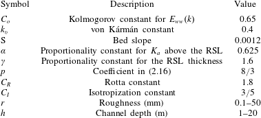
Model parameters and the range of values used in the numerical integration of the CSB model. Unless otherwise stated, the flow is stationary and uniform at very high Reynolds number in a wide channel, so that
 $R_{h}\approx h$
. Combinations of slope, water depth and roughness height were chosen to ensure a roughness Reynolds number
 $Re^{\ast }>$
200, so that the exponential cutoff in the viscous sublayer can be reasonably neglected in the CSB formulation.

To investigate low-wavenumber adjustments to
 $E_{ww}(k)$
, several scenarios were considered (see figure 3). First, the
 $u(z)$
was evaluated assuming a constant energy spectrum (E1) for
 $k<K_{a}$
(regimes I and II) and the Kolmogorov spectrum for
 $k>K_{a}$
(regime III). Second, the
 $E_{ww}(k)$
was set to zero for
 $k<K_{c}=1/(\unicode[STIX]{x1D6FD}h)$
and calculations were conducted for different values of
 $\unicode[STIX]{x1D6FD}=0.9,2.5,100$
(case E2). Finally,
 $E_{ww}(k)$
was assumed to vary linearly from 0 to
 $K_{c}$
with a slope of
 $p=8/3$
(case E3). The numerical integrations were conducted for
 $r$
varying between 0.1 mm and 50 mm, and
 $h$
varying between 1 and 20 m for illustration. In all cases, the TKE budget is assumed to be in equilibrium throughout, so that production and dissipation of TKE are balanced when computing
 $\unicode[STIX]{x1D716}(z)$
. While a TKE balance between only production and dissipation is unlikely in the entire RSL and in the outer layer of the channel (Pope Reference Pope2000), it was shown elsewhere (Katul & Manes Reference Katul and Manes2014; McColl et al.
Reference McColl, Katul, Gentine and Entekhabi2016) that the effect of this imbalance has minor impact on the shape of
 $u(z)$
.
3.1 Effect of low-wavenumber adjustments of
 $E_{ww}(k)$
on
$u(z)$


Mean velocity profiles obtained under different
 $r$
and
 $h$
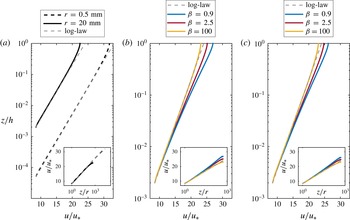
scenarios are compared with the logarithmic law (figure 4) to assess how low wavenumbers in
 $E_{ww}(k)$
shape
 $u(z)$
. The different low-wavenumber
 $E_{ww}(k)$
models are then assessed by the agreement between the modelled
 $f$
versus
 $r/R_{h}$
curves with the Strickler scaling (figure 5), the Colebrook equation and the virtual Nikuradse (VN) formula (Yang & Joseph Reference Yang and Joseph2009).
Velocity profiles for cases (a) E1, (b) E2 and (c) E3. The impact of different break points
 $K_{c}=(\unicode[STIX]{x1D6FD}h)^{-1}$
on
 $u(z)$
is shown in (b) and (c) for cases E2 and E3 respectively. Case E1 is illustrated for different roughness sizes
 $r$
, while cases E2 and E3 are shown for
 $r=20$
mm. Results are shown for
 $S=0.0012$
and
 $h=10$
m. The classical log law
 $u/u_{\ast }=8.5+(1/k_{v})\log (z/r)$
for a rough wall is also shown for comparison (dashed grey lines).

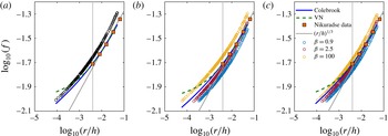
Comparison between
 $f=8f_{d}$
(circles) and the Strickler scaling
 $(r/h)^{1/3}$
(grey line) for cases (a) E1, (b) E2 and (c) E3. The impact of different break points
 $K_{c}=(\unicode[STIX]{x1D6FD}h)^{-1}$
on
 $f$
is shown in (b) and (c) for cases E2 and E3 respectively. Results are shown for
 $r$
varying between 0.1 and 50 mm,
 $h$
between 1 and 20 m, and bed slope
 $S$
set to 0.0012. Numerical results are shown for
 $r/h$
values that ensure
 $Re_{\ast }>200$
and
 $Fr<1$
. Colebrook’s formula (blue solid line) and predictions from the virtual Nikuradse (VN) model (green dashed line) are featured to illustrate the plausible range of deviations from Strickler scaling across numerous experiments. Nikuradse’s data for high
 $Re$
where
 $f$
is independent of
 $Re$
are also shown for reference (orange squares, digitized from Gioia & Chakraborty (Reference Gioia and Chakraborty2006)) so as to illustrate the range in
 $r/h$
considered in the CSB approach versus the original experiments by Nikuradse. The dotted grey lines indicate the smallest relative roughness explored by Nikuradse.

For the flow region above the roughness elements, all of the assumed energy spectra result in plausible mean velocity profiles that display a logarithmic region, with an apparent increase in the wake effect as
 $\unicode[STIX]{x1D6FD}$
decreases (i.e. higher break point
 $K_{c}$
), as shown in figure 4. This finding is consistent with results for smooth pipes, where the low-frequency correction to the Kolmogorov spectrum has a key influence on the magnitude of the outer wake in the mean velocity profile (Katul & Manes Reference Katul and Manes2014). This analysis suggests that the choice of the spectral break point
 $K_{c}$
influences
 $u(z)$
more when compared with the precise scaling laws in
 $E_{ww}$
for
 $K\in [0,K_{c}]$
and that a significant contribution of low-wavenumber eddies is required in the spectra to reproduce the outer wake. In further support of this claim, by imposing
 $K_{c}=K_{a}=(\unicode[STIX]{x1D6FC}z)^{-1}$
(i.e. setting to zero all of the large-scale eddies energy), the wakes in the computed mean velocity profiles
 $u(z)$
are completely off (not shown here). All of these findings confirm that application of the
 $E_{1}$
spectral shape to derive Manning’s formula in (2.27) was a reasonable assumption.
All of the energy spectral models result in
 $f_{d}$
exhibiting a Strickler scaling restricted only to an intermediate range of
 $r/h$
values (figure 5). This result is robust for any (sensible) choice of free parameters contained in the CSB model. Such deviations from the Strickler scaling predicted by the proposed CSB approach are to be expected and are physically plausible. To illustrate, friction factor calculations conducted using Colebrook’s empirical formula
 $f^{-1/2}=-2\log [r/(14.8R_{h})]$
as well as the VN model for granular beds at very high bulk Reynolds number (
 $f=0.1781(r/2R_{h})^{0.4678}+0.0098$
) along with Nikuradse’s original data are featured in figure 5. Encouragingly, the CSB model predictions of
 $f_{d}$
are close to the VN equation, which is, to date, the best fit of Nikuradse’s data on pipes with walls roughened with granular roughness. The CSB model also predicts an approximate Strickler scaling in the range of
 $r/h$
values originally explored by Nikuradse. This acceptable agreement between experimental and model results further corroborates the applicability of the proposed CSB model.
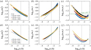
Variation of the proportionality constants (a,d)
 $\unicode[STIX]{x1D6FC}_{2}$
and (b,e)
 $\unicode[STIX]{x1D6FC}_{1}$
(at
 $z=\unicode[STIX]{x1D6FE}r$
) as a function of
 $r/h$
in cases E1, E2 and E3. The
 $-1/6$
and
 $1/6$
Strickler scalings are shown for comparison (grey lines in (a,d) and (b,e)). (c,f) Variation of the product
 $\unicode[STIX]{x1D6FC}_{1}\unicode[STIX]{x1D6FC}_{2}$
as a function of
 $r/h$
. Results are shown for
 $r$
varying between 0.1 and 50 mm,
 $h$
between 1 and 20 m, and bed slope
 $S$
set to 0.0012. Numerical results are shown for
 $r/h$
values that ensure
 $Re_{\ast }>200$
and
 $Fr<1$
. The dotted grey lines indicate the smallest relative roughness explored by Nikuradse. The green dashed line in (c) represents the mean value
 $\unicode[STIX]{x1D6FC}_{1}\unicode[STIX]{x1D6FC}_{2}=10^{-1.26}$
for case E1 used in the evaluation of
 $n$
in figure 7.

3.2 Relations between local and bulk variables
The
 $\unicode[STIX]{x1D6FC}_{1}$
and
 $\unicode[STIX]{x1D6FC}_{2}$
evaluated at
 $z=\unicode[STIX]{x1D6FE}r$
with
 $\unicode[STIX]{x1D6FE}=1.6$
are presented in figure 6 as a function of
 $r/h$
for cases E1, E2 and E3. In principle, to recover Strickler’s scaling in (2.28),
 $\unicode[STIX]{x1D6FC}_{1}\sim (r/h)^{1/6}$
and
 $\unicode[STIX]{x1D6FC}_{2}\sim (r/h)^{-1/6}$
are necessary, so that their product becomes independent of
 $r/R_{h}$
. Consistent with figure 5, these scaling rules appear to hold for intermediate values of
 $r/h$
. Despite these deviations, and while the model calculations suggest that
 $\unicode[STIX]{x1D6FC}_{1}$
and
 $\unicode[STIX]{x1D6FC}_{2}$
do not strictly obey the Strickler scaling, they follow opposite power-law behaviours, as they should. That is,
 $\unicode[STIX]{x1D6FC}_{1}\unicode[STIX]{x1D6FC}_{2}$
becomes only weakly dependent on
 $r/h$
(figure 6
c). Specifically, for case E1 in figure 6(c), the product
 $\unicode[STIX]{x1D6FC}_{1}\unicode[STIX]{x1D6FC}_{2}$
ranges between 0.048 and 0.08, resulting in only a weak variation of
 $\sqrt{\unicode[STIX]{x1D6FC}_{1}\unicode[STIX]{x1D6FC}_{2}}\in [0.22;0.28]$
with
 $r/R_{h}$
. The results from the CSB presented in figures 5 and 6 confirm that Strickler’s scaling (i.e.
 $n\sim r^{1/6}$
or
 $f_{d}\sim (r/R_{h})^{-1/3}$
) represents a reasonable but inaccurate scaling law relating friction factors with roughness size for a wide range of
 $r/R_{h}$
.
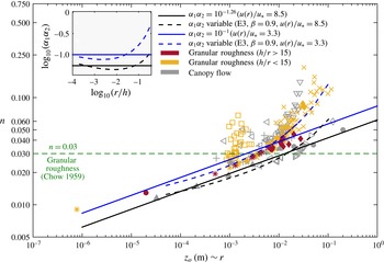
Comparison between measured and modelled Manning’s roughness coefficient
 $n$
using (2.28) and literature values. Results from (2.28) are shown for
 $\unicode[STIX]{x1D6FC}_{1}\unicode[STIX]{x1D6FC}_{2}$
constant (solid line) and set equal to the mean values 10
 $^{-1.26}$
(black) and 10
 $^{-1}$
(blue) obtained from the E1 spectrum imposing
 $u(r)/u^{\ast }$
=8.5 and 3.3 respectively (see the 10
 $^{-1.26}$
line in figure 6
c). Values of
 $n$
assuming a variable shape of
 $\unicode[STIX]{x1D6FC}_{1}\unicode[STIX]{x1D6FC}_{2}$
(spectrum E3,
 $\unicode[STIX]{x1D6FD}=0.9$
) are shown for qualitative (or trend) comparison (dashed lines, black and blue for the two different boundary conditions). The model results for the variable
 $\unicode[STIX]{x1D6FC}_{1}\unicode[STIX]{x1D6FC}_{2}$
are computed assuming
 $z_{0}=r/2$
. Data for granular roughness are shown for deep and shallow stream flows (red and yellow symbols respectively). Data from canopy flow experiments are also shown for comparison (grey symbols). For dense canopies, flume and wind tunnel experiments using rod canopies and field experiments in the RSL of tall forests suggest
 $u/u_{\ast }=3.3$
at the canopy top. The green dashed line shows the
 $n=0.03$
value for granular roughness given by Chow (Reference Chow1959). Symbols refer to different studies: (●) Katul et al. (Reference Katul, Wiberg, Albertson and Hornberger2002), (▴) Poggi et al. (Reference Poggi, Porporato, Ridolfi, Albertson and Katul2004), (
 $+$
) López & García (Reference López and García2001), (♢) Meijer & Van Velzen (Reference Meijer and Van Velzen1999), (▹) Ghisalberti & Nepf (Reference Ghisalberti and Nepf2004), (◃) Murphy, Ghisalberti & Nepf (Reference Murphy, Ghisalberti and Nepf2007), (▵) Yang & Choi (Reference Yang and Choi2010), (▿) Cheng (Reference Cheng2011), (
 $\star$
) Dunn, López & García (Reference Dunn, López and García1996), (○) Nezu & Sanjou (Reference Nezu and Sanjou2008), (▪) Manes et al. (Reference Manes, Pokrajac and McEwan2007), (♦) Hey (Reference Hey1979), (*) Colosimo, Copertino & Veltri (Reference Colosimo, Copertino and Veltri1988), (▫) Bathurst, Simons & Li (Reference Bathurst, Simons and Li1981), (
 $\times$
) Bathurst (Reference Bathurst1985).

4 Evaluation of Manning’s roughness coefficient for permeable and impermeable rough surfaces
To further evaluate (2.28) for
 $n$
where the roughness elements can deviate from their assumed shape in figure 1, a comparison with literature values is provided in figure 7. The data span seven decades of roughness values. For uniformity in characterizing
 $r$
across various roughness types, the following published datasets for
 $n$
as a function of momentum roughness height
 $z_{o}$
(
 ${\sim}r$
) for channel and atmospheric flows are used: (i) rigid canopy elements (Konings, Katul & Thompson (Reference Konings, Katul and Thompson2012), original data from Dunn et al. (Reference Dunn, López and García1996), Meijer & Van Velzen (Reference Meijer and Van Velzen1999), López & García (Reference López and García2001), Ghisalberti & Nepf (Reference Ghisalberti and Nepf2004), Poggi et al. (Reference Poggi, Porporato, Ridolfi, Albertson and Katul2004), Murphy et al. (Reference Murphy, Ghisalberti and Nepf2007), Nezu & Sanjou (Reference Nezu and Sanjou2008), Yang & Choi (Reference Yang and Choi2010), Cheng (Reference Cheng2011)); (ii) data for many bluff-rough surface covers including both vegetated and granular surfaces from Katul et al. (Reference Katul, Wiberg, Albertson and Hornberger2002) (original data from Chow (Reference Chow1959), Brutsaert (Reference Brutsaert1982)); (iii) measurements from Katul et al. (Reference Katul, Wiberg, Albertson and Hornberger2002) including data for shallow gravel streams by Hey (Reference Hey1979), Bathurst (Reference Bathurst1985), Colosimo et al. (Reference Colosimo, Copertino and Veltri1988) and laboratory flumes by Bathurst et al. (Reference Bathurst, Simons and Li1981); (iv) laboratory flume experiments from Manes et al. (Reference Manes, Pokrajac and McEwan2007). Where not available,
 $z_{o}$
is estimated as (Katul et al.
Reference Katul, Wiberg, Albertson and Hornberger2002)
 $$\begin{eqnarray}\displaystyle z_{o}=\frac{h}{\exp \left(1+k_{v}\sqrt{\displaystyle \frac{8}{f}}\right)}, & & \displaystyle\end{eqnarray}$$
where
 $h$
and
 $f$
are measured or reported in the experiments. The data here include rigid but densely arrayed rods, permeable rough canopies and uniform gravel beds with various diameters and thicknesses. The Strickler scaling did not originally cover such roughness shapes and was restricted to single-sized grains. The derivation here makes it clear that the existence of an RSL with a thickness that scales with
 $r$
(or
 $z_{o}$
if
 $r$
is ambiguously defined) may still follow an approximate Strickler scaling for
 $n$
, although several deviations for shallow flows and canopy elements are apparent. Manning’s
 $n$
is evaluated by means of (2.28) assuming a constant
 $\unicode[STIX]{x1D6FC}_{1}\unicode[STIX]{x1D6FC}_{2}=10^{-1.26}$
(see figure 6, E1 spectrum and boundary condition equal to
 $u(r)/u_{\ast }=8.5$
) and compared with literature values (figure 7, black solid line). Since the roughness height
 $r$
is not known for all experiments, the comparison is performed assuming
 $z_{o}\sim r$
(Raupach, Hughes & Cleugh Reference Raupach, Hughes and Cleugh2006). It should be noted that the slope, water level height and boundary conditions (all influencing the value of
 $\unicode[STIX]{x1D6FC}_{1}\unicode[STIX]{x1D6FC}_{2}$
) vary for each lab/field study, and the comparison with (2.28) is mainly featured for qualitative assessment of trends. The acceptable agreement between modelled and measured roughness coefficients shows that the derivation of Manning’s formula using the CSB model provides acceptable values for
 $n$
even when
 $r$
varies by seven orders of magnitude. Furthermore, the comparison between modelled and measured
 $n$
also demonstrates that framing the CSB in the RSL above the roughness elements but below the logarithmic region reduces the sensitivity of the flow statistics to the precise geometry of the roughness elements provided that it can be encoded in a single effective roughness length
 $r\sim z_{o}$
. The model provides a reasonable estimate of
 $n$
for granular roughness in deep streams (i.e. the conditions under which the CSB model was framed), while deviations can be observed for vegetated surfaces and shallow flows (
 $h/r<15$
), as already well known from extensive literature on flow resistance in open channel flows (see, e.g. Ferguson (Reference Ferguson2010) and references therein). Considering different boundary conditions and the dependence of
 $\unicode[STIX]{x1D6FC}_{1}\unicode[STIX]{x1D6FC}_{2}$
on
 $r$
may explain such deviations. In particular, imposing
 $u(r)/u_{\ast }=3.3$
(typical for dense canopy flows) provides Manning’s roughness coefficient
 $n$
in better agreement with the measured values.
5 Discussion and conclusions
GB02 proposed the first theoretical derivation for two well-known empirical laws in hydraulics: (i) the Manning equation and (ii) the associated Strickler scaling for the roughness coefficient
 $n$
. The work by GB02 provided a new strategy to address theoretically what has always been an empirical matter. However, despite its significance, simplicity, elegance and appeal, their work required revisions and critical appraisal. In deriving Manning’s formula, GB02 adopted a series of assumptions which have been critically investigated here considering known physics of rough-wall turbulent flows. These include (i) assuming the applicability of Kolmogorov scaling for velocity fluctuations immediately adjacent to roughness elements, (ii) the hypothesis that
 $\unicode[STIX]{x1D70F}\sim \unicode[STIX]{x1D70C}Vu_{r}$
, where
 $u_{r}$
represents the velocity scale of an eddy of size
 ${\approx}r$
, (iii) the hypothesis that eddies of size
 $r$
are the major players in momentum transfer in the near-wall region, (iv) the mean TKE dissipation rate scales as
 $V^{3}/R_{h}$
with a scaling factor independent of
 $r/h$
near the roughness elements. GB02 have also assumed, although implicitly (but explicitly in a subsequent paper), that the mean velocity gradient at the roughness tops scales as
 $V/r$
and that the associated scaling factor is also independent of
 $r/h$
.
The present paper first demonstrated that assumption (iv) is incorrect and that the scaling functions pertaining to the TKE dissipation rate and the mean velocity gradient must depend on
 $r/R_{h}$
. When this dependence is taken into account within the GB02 derivation, Manning’s equation can still be recovered but not the Strickler scaling as argued by GB02.
The new CSB approach proposed herein allows for the relaxation of hypotheses (i), (ii) and (iii) as it moves the point of analysis at the cross-over between the RSL and logarithmic layer, where Kolmogorov scaling for inertial subrange turbulence is applicable, it computes the turbulent shear stress directly from the integration of the co-spectrum and it incorporates all of the population of eddies that contribute to momentum transfer in the RSL, including very large eddies (i.e. eddies that exceed
 $R_{h}$
in size).
While relaxing the hypotheses pertaining to GB02, the CSB approach introduces some new ones. These include neglecting wall-blocking and flux-transfer term effects in the CSB budget and assuming equilibrium between production and dissipation of TKE throughout the flow domain. The former was explored (not shown), and proved to be a more than reasonable assumption, whereas the latter was addressed in preceding papers (Katul & Manes Reference Katul and Manes2014; McColl et al.
Reference McColl, Katul, Gentine and Entekhabi2016) and was also shown to be acceptable. Perhaps the most stringent hypothesis of the proposed CSB approach is on the shape of the vertical velocity spectrum. This is seldom available in the literature, and, when it is, it relates to 1-D spectra which suffer major distortions induced by the use of Taylor’s frozen turbulence hypothesis and aliasing effects. This lack of information required a speculative approach with assumed spectral shapes especially for what concerns the low-wavenumber range. We therefore assumed the existence of an inertial subrange characterized by a Kolmogorov spectrum at high wavenumbers and a flat spectrum for the lower wavenumbers. The cross-over between the two regimes is dictated by scales commensurate with the elevation
 $z$
above the bed (but
 $r$
in proximity of the wall). This simplified version of the spectrum allowed for analytical foresight of the problem, leading to Manning’s equation from the CSB and momentum budget equations.
To evaluate this assumed choice for the vertical velocity spectrum, numerical calculations were performed to explore how the full CSB model responded to different and more complex spectral shapes. In particular, a spectral decay at the low-wavenumber end of the spectrum was introduced, and we varied extensively the size of the flat spectral region at low wavenumbers. The results show that the model is weakly sensitive to how the spectrum decays at low wavenumbers. To reproduce realistic mean velocity profiles in the outer layer, the flat region (i.e. the contribution of large eddies) must be significant in extent. Both results work in favour of the simplified version of the spectrum used to derive Manning’s equation. Even though none of the investigated spectral shapes allowed a full recovery of the Strickler scaling across all of the
 $r/R_{h}$
ranges considered, the CSB predicted departures from Strickler scaling that are consistent with well-established equations such as Colebrook’s formula and the VN model.
Acknowledgements
Support from the US National Science Foundation (FESD EAR-1338694, NSF-EAR-1344703, NSF-CBET-1033467, NSF-EAR-1331846, NSF-EAR-1316258, NSF-DGE-1068871 through Duke WISeNet) and the USDA Agricultural Research Service cooperative agreement (58-6408-3-027) is acknowledged. C.M. acknowledges support from Compagnia San Paolo.