

Introduction
To many Americans, achieving the national dream means gaining personal wealth, being happy and satisfied with life. A popular belief among Americans has been that money is essential for happiness, but not all people see it this way. People's perceptions of happiness vary widely even among those who live under similar economic and financial conditions. Therefore, to what degree money can (or cannot) buy happiness, or more specifically, under what circumstances money promotes happiness is not self-evident (George Reference George, Cutler, Gregg and Lawton1992). The factors that influence people's perception of happiness have long been the focus of scholars and philosophers. Social scientists in particular have devoted a great deal of effort to the topic (e.g. Campbell, Converse and Rogers Reference Campbell, Converse and Rogers1976; Diener Reference Diener1984; Feist et al. Reference Feist, Bodner, Jacobs, Miles and Tan1995; George and Bearon Reference George and Bearon1980; Myers and Diener Reference Myers and Diener1995). Although social gerontologists have for years researched the relationship between age and ageing and happiness, life satisfaction and subjective wellbeing, most studies have centred only on older adults (Cutler Reference Cutler, Cutler, Gregg and Lawton1992). Research to date has yet to offer conclusive findings on the effect of age on happiness (Felton Reference Felton1987; La Barbera and Gürhan Reference La Barbera and Gürhan1997; Shmotkin Reference Shmotkin1990; Stock et al. Reference Stock, Okun, Haring, Witter and Light1983; Yang Reference Yang2008).
This study focuses on the relationships between money, happiness and age among American adults. More specifically, it aims to increase understanding of the relationship between money and happiness across three commonly recognised adult age groups: young (18–44 years), middle-age (45–64 years) and older (65 or more) (cf. Cutler Reference Cutler, Cutler, Gregg and Lawton1992). The research question addressed is: does the relationship between money and happiness differ by age group?
Literature review
According to Maddox (Reference Maddox, Cutler, Gregg and Lawton1992), studies of happiness and satisfaction have been merged with studies of wellbeing since the work of Campbell, Converse and Rogers (Reference Campbell, Converse and Rogers1976). One result is that researchers generally use the rubric of subjective wellbeing to include both studies of happiness, which concentrate on the balance between the positive and negative components of mood, and studies of satisfaction that focus on the extent to which hopes and aspirations are perceived to be fulfilled (Diener Reference Diener1984; George Reference George, Cutler, Gregg and Lawton1992; Maddox Reference Maddox, Cutler, Gregg and Lawton1992).
Researchers have devoted a great deal of effort to studying happiness or subjective wellbeing (Campbell, Converse and Rogers Reference Campbell, Converse and Rogers1976; Di Tella, MacCulloch and Oswald Reference Di Tella, MacCulloch and Oswald2003; Diener Reference Diener1984; Feist et al. Reference Feist, Bodner, Jacobs, Miles and Tan1995; Frey and Stutzer Reference Frey and Stutzer2002; George and Bearon Reference George and Bearon1980; Myers and Diener Reference Myers and Diener1995; Robinson and Martin Reference Robinson and Martin2008; Tran Reference Tran1992; Yang Reference Yang2008). Some studies have examined subjective wellbeing from an aggregate aspect; that is, they focus not on individuals but on social groups, such as countries or specific populations. Most such research has centred on trends in subjective wellbeing in an entire society or in populations with certain characteristics (e.g. Myers and Diener Reference Myers and Diener1995; Rodgers Reference Rodgers1982), or has compared mean subjective wellbeing and other factors (such as gross domestic product) among countries (e.g. Diener, Diener and Diener Reference Diener, Diener and Diener1995; Layard Reference Layard2005; Myers and Diener Reference Myers and Diener1995). Layard (Reference Layard2005), for example, argued although richer people tend to be happier than poor people, increases in wealth in already rich countries have not increased happiness over the past several decades. Other individual-level factors, such as family, friendship and health should not be overlooked.
A large body of research focuses on identifying factors associated with subjective wellbeing at the individual level. There are many ways to examine the associations. Some studies concentrate on the directions (positive or negative) and magnitude that particular variables (e.g. health, gender, marital status, and so on) have on subjective wellbeing, and many report the predictive (or explanatory) power of the combination of a set of variables. For example, Fengler and Jensen (Reference Fengler and Jensen1981) assessed the effects of objective conditions and subjective perceptions of factors such as income, health, transportation and housing on life satisfaction of urban and non-urban older people and found that subjective perceptions were better predictors of life satisfaction. Ruffing-Rahal and Anderson (Reference Ruffing-Rahal and Anderson1994) developed a regression model to predict subjective wellbeing, and reported that the combination of five significant variables (number of health concerns, perceived ability actively to practise religion, age, length of residence at present address and education) accounted for 34 per cent of the variance in subjective wellbeing. La Barbera and Gürhan (Reference La Barbera and Gürhan1997) studied the effects of materialism and religiosity on subjective wellbeing. They found materialism to be positively related to subjective wellbeing among people with low religiosity but negatively related to subjective wellbeing among people with high religiosity. In addition, studies have proposed and examined the possible causal relationships between the associated factors and subjective wellbeing (e.g. Donnenwerth and Petersen Reference Donnenwerth and Petersen1992; Elwell and Maltbie-Crannell Reference Elwell and Maltbie-Crannell1981; Liang Reference Liang1982; Markides and Martin Reference Markides and Martin1979; McKenzie and Campbell Reference McKenzie and Campbell1987).
In the literature, at least nine major variables are considered to be correlates of subjective wellbeing, including income, other socio-economic status attributes (such as education and social status), health, age, gender, race, work/employment, marital status and social interaction (Beatty and Tuch Reference Beatty and Tuch1997; Burton et al. Reference Burton, Rushing, Ritter and Rakocy1993; Campbell, Converse and Rogers Reference Campbell, Converse and Rogers1976; Diener Reference Diener1984; Feist et al. Reference Feist, Bodner, Jacobs, Miles and Tan1995; George and Bearon Reference George and Bearon1980; McKenzie and Campbell Reference McKenzie and Campbell1987; Mookherjee Reference Mookherjee1992; Myers and Diener Reference Myers and Diener1995; Shmotkin Reference Shmotkin1990; Stevens Reference Stevens1993). Although all the major correlates are important for studying subjective wellbeing, this study focuses on two variables, income and age.
Income
Most subjective wellbeing studies have used income as a proxy for money or wealth (George Reference George, Cutler, Gregg and Lawton1992; Yang Reference Yang2008). George (Reference George, Cutler, Gregg and Lawton1992) reviewed more than 20 studies and found that the bivariate relationship between income and subjective wellbeing to be positive and often strong. The relationship between income and subjective wellbeing is less apparent, however, in multivariate relationships. For example, Elwell and Maltbie-Crannell (Reference Elwell and Maltbie-Crannell1981) reported a significant direct effect between income and subjective wellbeing for older men but not for older women. La Barbera and Gürhan (Reference La Barbera and Gürhan1997) found that income was positively correlated with subjective wellbeing for people with low religiosity but negatively correlated to subjective wellbeing for people with high religiosity. Veenhoven (Reference Veenhoven, Strack, Argyle and Schwarz1991) suggested that income helped people meet certain needs and, therefore, should be a cause of subjective wellbeing, but Myers and Diener (Reference Myers and Diener1995) suggested that although the absence of income could be misery, the relationship between income and subjective wellbeing by no means should be a positive linear one. Researchers have also argued the importance of social comparison in examining the relationship between income and happiness (e.g. Ferrer-i-Carbonell Reference Ferrer-i-Carbonell2005; George Reference George, Cutler, Gregg and Lawton1992; Layard Reference Layard2005; Liang and Fairchild Reference Liang and Fairchild1979). More specifically, researchers indicate that individual's perception of income is dependent on his/her own income in relation to the past as well as income of other people. Subjective wellbeing is influenced by the perception of income, in addition to actual income (e.g. Ferrer-i-Carbonell Reference Ferrer-i-Carbonell2005).
Age
According to Felton (Reference Felton1987) and La Barbera and Gürhan (Reference La Barbera and Gürhan1997), studies during the 1950s and 1960s generally reported a negative relationship between age and subjective wellbeing, while during the early 1970s, researchers found no relationship between age and subjective wellbeing, although recent studies have found a positive relationship between age and subjective wellbeing (e.g. Shmotkin Reference Shmotkin1990). George (Reference George, Cutler, Gregg and Lawton1992, Reference George, Binstock and George1996) suggested that the relationship between age and subjective wellbeing may not be linear, a claim that has recently been supported by empirical evidence (e.g. Fischer Reference Fischer2009; Yang Reference Yang2008).
Data, variables and methods
This study carried out a secondary analysis of the cumulative data from the United States General Social Surveys (GSS) from 1972 to 2006 (Davis, Smith and Marsden Reference Davis, Smith and Marsden2006). To explore the relationship between money and happiness across various age groups, the following variables were used: happiness and a set of explanatory variables (which have been identified as major correlates of subjective wellbeing) including gender, race, age, marital status, education, income, perceived health condition, civic organisation memberships, attendance of religious services. The dependent variable happiness (HAPPY) was taken from the responses to a single question in the survey, ‘Taken all together, how would you say things are these days – would you say that you are very happy, pretty happy, or not too happy?’ (Davis, Smith and Marsden Reference Davis, Smith and Marsden2006). This item has been used in many studies to represent global or overall sense of subjective wellbeing (e.g. Beck Reference Beck1982; Donnenwerth and Petersen Reference Donnenwerth and Petersen1992; Michalos Reference Michalos2004; Robinson and Martin Reference Robinson and Martin2008; Yang Reference Yang2008). As suggested in the literature, the validity and reliability of single-item measures are adequate (e.g. Veenhoven Reference Veenhoven1996). Instead of treating the responses of the happiness variable as ordinal, this study combined ‘very happy’ and ‘pretty happy’ to form a binary dependent variable that distinguished those who were ‘happy’ (‘very’ or ‘pretty’ happy) as against the ‘unhappy’ (‘not too’ happy').
Like most previous studies of financial status and subjective wellbeing, income was used as the proxy for the former as the independent variable of interest. The GSS collects the respondent's individual income as well as household income. Given that many respondents did not report individual income, household income was used for the analysis. The household income variable (REALINC) was collected from 1972 to 2006, and the National Opinion Research Center (NORC) has converted each of the dollar values into the 1986 inflation-adjusted equivalent (Davis, Smith and Marsden Reference Davis, Smith and Marsden2006). The income values are therefore comparable throughout the survey years. Also the GSS income variable is in categories, so the values for REALINC are the midpoints of the categories and, for the open-ended upper category the mean of the Pareto curve (Ligon Reference Ligon1989). Many previous subjective wellbeing studies simply used the variable household income without taking household size into account (e.g. Beck Reference Beck1982; Doyle and Forehand Reference Doyle and Forehand1984; Headey, Veenhoven and Wearing Reference Headey, Veenhoven and Wearing1991; Yang Reference Yang2008). It is misleading not to take into account household size because a person living alone with an income of $25,000 clearly has a different level of material wellbeing from people living in a five-person household with the same income. This study used a simple equivalised income, now widely promoted by the Organisation for Economic Co-operation and Development (OECD 2008), that divides household income by the square root of the size of the household (HOMPOP). This study used both household income and the equivalised income for the comparisons. Given the positive skew of the two income distributions, the variables were transformed by taking the logarithm.
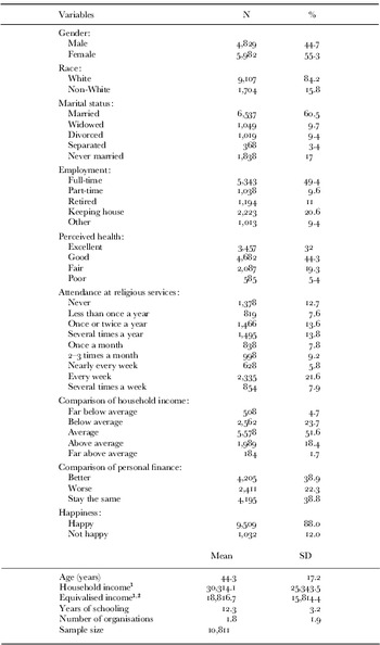
The other variables used in the analysis are itemised with their categories in Table 1. Most are standard measures and self-evident, but some require further explanation. The respondents' health status (HEALTH) is the GSS self-assessment measure, being the responses to the question, ‘would you say your own health, in general, is excellent, good, fair, or poor?’ (Davis, Smith and Marsden Reference Davis, Smith and Marsden2006). Previous studies have found this variable to be a strong correlate of subjective wellbeing (e.g. Hennon and Burton Reference Hennon and Burton1986; Tran Reference Tran1992). Turning to work or occupational status, the ‘other’ category includes ‘temporarily not working’ and ‘unemployed’.
Sample characteristics

Note: SD: standard deviation. 1. Annual in US dollars at 1986 value. 2. Equivalised income of an individual in a household.
The social interaction measure follows Beatty and Tuch (Reference Beatty and Tuch1997) and is based on two variables, the number of voluntary civic organisations the respondent belonged to (MEMNUM), and the frequency of attendance at religious services (ATTEND). The organisations included fraternal groups, service clubs, veterans' groups, political clubs, labour unions, sports groups, youth groups, school service groups, hobby or garden clubs, school fraternities or sororities, nationality groups, farm organisations; literary, art, discussion or study groups; professional or academic societies, church-affiliated groups, and any other groups. The question on religious service participation is, ‘how often do you attend religious services?’ The available responses were ‘never’, ‘less than once a year’, ‘about once or twice a year’, ‘several times a year’, ‘about once a month’, ‘2–3 times a month’, ‘nearly every week’, ‘every week’ and ‘several times a week’. Since each of these variables represented a different domain of social interaction, they were included as two separate variables in the analysis.
A social comparison measure was derived from two GSS variables (Davis, Smith and Marsden Reference Davis, Smith and Marsden2006) based, respectively, on the responses to two questions: ‘during the last few years, has your financial situation been getting better, worse, or has it stayed the same?’ (comparison of personal finance), and ‘compared with American families in general, would you say your family income is far below average, below average, average, above average, or far above average?’ (comparison of household income). These two variables have been used in prior studies as indicators of social comparison or relative deprivation, especially in studies of people's financial satisfaction (Hsieh Reference Hsieh2001, Reference Hsieh2003; Liang and Fairchild Reference Liang and Fairchild1979). Since each of these variables represented a different domain of social comparison, they were included as two separate variables in the analysis. In addition, the Consumer Price Index (CPI) compiled by the US Bureau of Labor Statistics (2006) and available on their website was included in the analysis to discount monetary value for inflation.
The GSS accumulated data set from 1972 to 2006 has 46,303 respondents with a happiness score, but there are missing data for other variables required for the analysis. Most importantly, the question on health was not asked in some survey years. There was also a substantial number of missing cases for income. After eliminating the years without the health measure and the cases with missing variables, the analysis sample comprises data for the years 1974, 1975, 1977, 1980, 1984, 1987–1991, 1993 and 1994. Altogether there were 10,811 respondents.
Methods
Before conducting the multivariate analysis and to circumvent multi-colinearity, the bivariate correlation matrix was reviewed to identify strong correlations among the independent variables (Allison Reference Allison1999b). A very high correlation (r=0.995) was identified between the survey year and the CPI, a function of incessant inflation during the survey years, which indicates that their distributions can be taken as identical. None of the other correlations exceeded |0.7|. Given that the data span 21 years, ‘year’ was included to capture possible period effects, and was preferred over the CPI.
Logistic regression models for each of three age groups were estimated to explore whether the relationship between income and happiness differed by age. At the first step (Model 1), the binary happiness variable was the dependent variable and the independent variables were age, (log) income and year. At the second step (Model 2), the rest of the socio-demographic and the health variables were added into the model, and at the final step (Model 3), the two social comparison variables were added. The conventional method to test for significance of differences in coefficients (e.g. Allison Reference Allison1999a) was used to compare if the effect of income varied significantly across the age groups. The following formula was used to compare two age groups:

where b i is the income coefficient on for age group i, b j is the income coefficient for group j, and se is the estimated standard error of b j.
The formula gives a chi-square statistic with one degree of freedom. Given that logistic regression was used in the analysis, Allison's (Reference Allison1999a) method of comparing logit coefficients across groups was also used to guard against the potential confounding effects of residual variation to confirm the results of these tests of significance.
Results
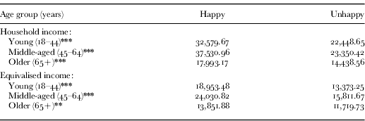
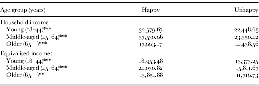
TABLE 1 shows the descriptive statistics of the sample respondents, and Table 2 shows the mean household income and mean equivalised income by happiness by the three age groups. The results presented in Table 2 indicate that those who were happy had significantly higher levels of household income than those who were unhappy across all three age groups. The results also indicate that among young and middle-aged adults, those who were happy had significantly higher levels of equivalised income than those who were unhappy. Among the older adults, however, the difference in equivalised income between those who were happy and those who were unhappy was not statistically significant.
Mean income (in 1986 dollars) by happiness and age group
Note: Sample size 10,811.
Significance levels: ** p<0.01, *** p<0.001.
Household income, age and happiness
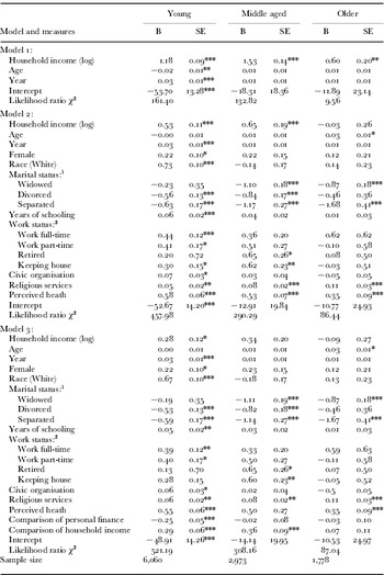
To further examine the research questions, multivariate logistic regression analysis was conducted. Table 3 shows the results of the regression of happiness on household income. Model 1 shows the results of the relationship between (log) household income and happiness after controlling for age and year. The results indicated that there was a significant positive relationship between household income and happiness for all three age groups. Model 2 shows the results of the relationship between (log) household income and happiness after controlling for age, year and additional socio-demographic variables. Model 2 results showed that after controlling for additional socio-demographic variables (including gender, race, marital status, education, working status, social interaction, and health), the significant positive relationship between household income and happiness remained for young and middle-aged adults. However, the significant positive relationship between household income and happiness for older adults disappeared after the inclusion of the additional socio-demographic variables. Model 3 shows the results of the relationship between (log) household income and happiness after controlling for age, socio-demographic variables and the social comparison variables. The Model 3 results show that after the inclusion of the social comparison variables, the significant positive relationship between household income and happiness disappeared for middle-aged adults but remained for young adults.
Estimated effects of household income and other variables on happiness

Notes: 1. ‘Never married’ category omitted. 2. ‘Other’ category omitted. B: Coefficient. SE: standard error.
Significance levels: * p<0.05, ** p<0.01, *** p<0.001.
Applying Equation (1) to the Model 1 results for household income, the chi-squared statistics (with one degree of freedom) for the difference in coefficients between young adults and older adults was 6.73 (p<0.01), between young adults and middle-aged adults 4.67 (p<0.05), and between middle-aged adults and older adults 14.62 (p<0.001) (Table 3). That is, the coefficient for household income in Model 1 was significant for all three age groups. Using the same formula for the results in Model 2, the chi-square difference in coefficients on (log) household income between young adults and older adults was 4.11 (p<0.05), between young adults and middle-aged adults 0.27 (p>0.05), and between middle-aged adults and older adults 4.57 (p<0.05). That is, the coefficient for household income in Model 2 was significantly larger for young and middle-aged adults than for older adults, but there was no significant difference between the coefficients for young adults and middle-aged adults. Although household income remained a significant predictor of happiness in Model 3 for young adults, there was no significant difference in the coefficients on household income across the three age groups when applying the same formula. Allison's (Reference Allison1999a) method (results not shown here) produced similar results.
Personal equivalised income, age and happiness
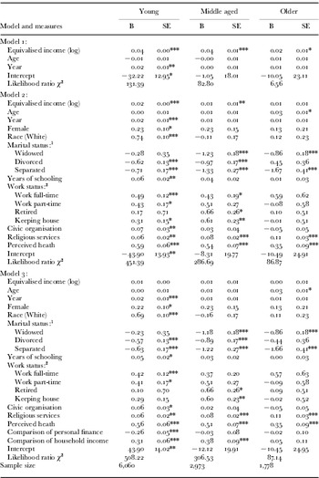
Table 4 shows the regression results of the relationship between personal equivalised incomes and happiness. Model 1 shows the results for the relationship between (log) equivalised income and happiness after controlling for age and year. The results indicated that there was a significant positive relationship between equivalised income and happiness for young and middle-aged adults, but no significant relationship between equivalised income and happiness for older adults. Model 2 shows the results of the relationship between (log) equivalised income and happiness after controlling for age, year and additional socio-demographic variables. Model 2 results showed that after controlling for additional socio-demographic variables (including gender, race, marital status, education, working status, social interaction, and health) the significant positive relationship between equivalised income and happiness remained for young and middle-aged adults.
Estimated effects of equivalised income and other variables on happiness

Notes: 1. ‘Never married’ category omitted. 2. ‘Other’ category omitted. B: Coefficient. SE: standard error.
Significance levels: * p<0.05, ** p<0.01, *** p<0.001.
Applying Equation (1) to the results in Model 1, the chi-squared difference in coefficients on (log) equivalised income between young adults and older adults was 10.4 (p<0.001), between young adults and middle-aged adults 0.61 (p>0.05), and between middle-aged adults and older adults 5.96 (p<0.001) (see Table 4). That is, the coefficient for equivalised income in Model 1 was significantly larger for young adults and middle-aged adults than for older adults, but there was no significant difference between the coefficients for young adults and middle-aged adults. Using the same formula for the results in Model 2 of Table 4, there was no significant difference in coefficients on (log) equivalised income across the three age groups. Again, Allison's (Reference Allison1999a) method (results not shown here) produced similar results. Since (log) equivalised income was not a significant predictor of happiness in Model 3 for all three age groups, no comparison of the coefficient was necessary.
Discussion
Using data from the United States General Social Surveys, this study has addressed the research question, ‘does the relationship between money and happiness vary by age group?’ The results show that even after controlling for all the major socio-demographic variables, income (no matter household income or equivalised income) had a significant positive association with happiness for young and middle-aged adults, but the relationship was not the same for older adults. After controlling for major socio-demographic variables, there was no evidence of a significant relationship between income (no matter household income or equivalised income) and happiness for older adults. In terms of the relationship between household income and happiness, the results showed that the coefficient was significantly smaller for older adults than for young or middle-aged adults in the model controlling for the major socio-demographic variables. The relationship between household income and happiness no longer differed significantly by age group when the social comparison variables were included. With respect to equivalised income, results show that the relationship between equivalised income and happiness did not vary significantly across age groups after controlling for major socio-demographic variables.
The empirical evidence presented in this study sheds new light on the age-old question, does money buy happiness? The results indicate that whether or not money (using income as proxy) associates with happiness in the United States of America depends on a person's age group as well as the income measure. More specifically, for young adults, household income significantly associates with happiness, even after controlling for socio-demographic variables and social comparison variables. Although equivalised income (household size-adjusted) significantly associated with happiness after controlling for socio-demographic variables among young adults, the association disappeared with the inclusion of social comparison variables. For middle-age adults, both household income and equivalised income significantly associated with happiness even after controlling for socio-demographic variables, but the association disappeared after controlling for the social comparison variables. For older adults, the association between income (both household income and equivalised income) and happiness disappeared after controlling for the socio-demographic variables.
To summarise, money, using household income as a proxy measure, had a significantly smaller effect on happiness for older adults than for young or middle-aged adults. No evidence suggests, however, that the association between household income and happiness differs across the three age groups after controlling for both socio-demographic and social comparison variables. When measured by equivalised income, the association between money and happiness did not vary significantly across the three age groups once socio-demographic variables are taken into account.
The results point to the importance of the selected income measure and the included control variables. If social comparison variables are taken into account (as controls), there is no evidence to suggest a significantly different relationship between money (using either household income or equivalised income as proxy) and happiness by age group. These results support the comparison income effect that previous researchers have identified (e.g. Ferrer-i-Carbonell Reference Ferrer-i-Carbonell2005) in examining the relationship between income and happiness. If, on the other hand, social comparison variables are not taken into account, it is important to recognise that the type of income selected would have consequences on whether or not one can assume a constant relationship between income and happiness at all ages. Assuming a constant relationship between income and happiness at all ages is problematic if household income is chosen, given the strong evidence that the relationship between (family) income and happiness is significantly weaker for older adults than for young or middle-aged adults. If equivalised income is chosen, then there does not appear to be any evidence against assuming a constant relationship between income and happiness across age groups. Using equivalised income in addition to household income, this study offered comparative results on the relationship between money and happiness. Equivalised income is not, however, without controversy. The two major issues associated with this equivalised income are: it assumes an equal share of income among all family members; and it does not take into account the age of various family members.
It should be noted that the GSS data used in the analysis were from repeated cross-sectional surveys. As from any such data, the findings could be influenced by ageing, period and cohort effects, so the results should be interpreted with caution. In addition, given the secondary analysis, two major issues should be borne in mind. First, this study dichotomised the responses of the dependent variable into ‘happy’ and ‘unhappy’ but most previous analyses have considered the level of happiness. The results of this study should be interpreted with caution when compared with other studies. Second, the available dependent and independent variables were limited. The relationship between money and happiness was assessed using only income as proxy for money in this study. It is clear that money or wealth covers more than just income. However, this study could analyse only the variables included in the GSS data set. Given the study's limitations, the findings are not conclusive. Future research should employ refined measures of happiness and examine more covariates for, as mentioned earlier, income is neither a comprehensive measure of material standing not does it fully account for self-rated wellbeing or happiness. Given the age effect in income and financial resources, it will be important to explore the relationships between happiness and other financial resources, in addition to income.