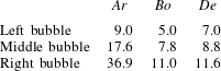
1. Introduction
The buoyancy-driven motion of a bubble rising through a viscoelastic fluid has been a subject of intense research for over four decades. The coupled and complex phenomena observed during this motion arise due to the impact of the viscoelastic nature of the fluid on the physics of the deformable free surface. More specifically, experiments have demonstrated that bubble motion is connected with (1) the formation of the inverted teardrop shapes, (Astarita & Apuzzo Reference Astarita and Apuzzo1965; Zana & Leal Reference Zana and Leal1977), (2) the appearance of the so-called negative wake, (Hassager Reference Hassager1979), and (3) the discontinuity in its rise velocity as its volume increases, (Astarita & Apuzzo Reference Astarita and Apuzzo1965; Leal, Skoog & Acrivos Reference Leal, Skoog and Acrivos1971). The latter effect is perhaps the most striking and fascinating one during the steady rise of a bubble in viscoelastic fluids. From the practical viewpoint, the mechanisms which lead to these phenomena and the resulting changes in the flow field around the deformable interface play an important role in determining the rates of heat and mass transfer from/to the bubble through its velocity and residence time, and the coalescence and patterns that many bubbles can form (Vélez-Cordero, Sámano & Zenit Reference Vélez-Cordero, Sámano and Zenit2012).
In an effort to explain the inverted teardrop shape, in an early theoretical work (Tiefenbruck & Leal Reference Tiefenbruck and Leal1980) studied the deviation from the spherical shape for slightly elastic liquids, under creeping flow conditions using perturbation expansions. This and other small deformation theories could predict only smooth prolate bubble shapes, but not the formation of a true tip or cusp, as has been observed in experiments. The difficulties that arise due to the kinematics of the free surface, coupled with the nonlinear character of the constitutive equations, made the numerical methods the only way to tackle this problem theoretically. In this direction, first Chilcott & Rallison (Reference Chilcott and Rallison1988) studied the rising of a ‘cylindrical’ bubble in a Boger-type fluid using the FENE-CR model. They showed that large extensional stresses develop at the rear stagnation point and extend radially for over 10 radii away. They argued that these should deform the free surface by pulling out the rear pole of the bubble, but in their calculations they did not allow for bubble shape deformations. Using the same constitutive model and boundary-fitted, orthogonal coordinates, Noh, Kang & Gary Leal (Reference Noh, Kang and Gary Leal1993) predicted deformed bubble shapes qualitatively similar to those observed in experiments, which they also attributed to the uniaxial straining flow in a direction normal to the rear pole of the bubble. However, they did not predict the tip formation, owing to numerical convergence problems. In addition to the axisymmetric shape of the bubble, three-dimensional shapes have been observed: Hassager (Reference Hassager1979) reported the change of a weakly cusped shape into a knife-edge shape with increasing bubble volume, while the work by Liu, Liao & Joseph (Reference Liu, Liao and Joseph1995) added more complicated shapes that could arise on its rear side. Very recently, You, Borhan & Haj-Hariri (Reference You, Borhan and Haj-Hariri2009) used the FENE-CR model to investigate reasons that might lead to deviation from the axisymmetric cusp shapes to more complex shapes. By performing stability and energy budget analysis on a base state of an axisymmetric cusped bubble, they determined that the only unstable eigenmode had a zero imaginary part and an azimuthal wavenumber equal to 2, which should result in a knife-edge shape. In the above, and other experimental studies, it is often clear that the 3D shapes are affected by the side and bottom walls of the containing vessel, especially considering the large and extended elastic stresses that develop on the side and rear of the bubble, and that for small ratios of bubble to container radius the occurrence of knife-edge shapes decreases.
The second experimental observation during bubble rise is the development of the ‘negative wake’, a term introduced by Hassager (Reference Hassager1979). The same flow structure was observed earlier by Sigli & Coutanceau (Reference Sigli and Coutanceau1977) and a little later by Bisgaard & Hassager (Reference Bisgaard and Hassager1982) and Bisgaard (Reference Bisgaard1983), who studied the settling of particles in shear-thinning viscoelastic fluids. Although a Newtonian fluid flows around a bubble or a sphere in the same direction as the translating object, a ‘negative wake’ appears in certain viscoelastic fluids, in which the fluid behind the settling sphere moves upwards and the fluid behind the rising bubble moves downwards, i.e. in both cases it moves opposite to the direction that the body moves. Due to the complex nature of the free surface, the ‘negative wake’ has been more extensively studied for settling spheres, both numerically and experimentally. This flow structure is experimentally observed only in viscoelastic fluids with shear-thinning viscosity, (Arigo & McKinley Reference Arigo and McKinley1998), while in Boger-type fluids (Arigo et al. Reference Arigo, Rajagopalan, Shapley and McKinley1995) only fairly extended wakes are observed. This is also supported by the numerical studies performed by Chilcott & Rallison (Reference Chilcott and Rallison1988) and Lunsmann et al. (Reference Lunsmann, Genieser, Armstrong and Brown1993) using the FENE-CR constitutive equation. The same distinction holds for rising bubbles in Boger fluids, where Vélez-Cordero et al. (Reference Vélez-Cordero, Sámano and Zenit2012) did not observe negative velocities downstream of the air bubbles they examined. In contrast, early numerical studies by Jin, Phan-Thien & Tanner (Reference Jin, Phan-Thien and Tanner1991) using the shear-thinning, Phan-Thien–Tanner model predicted the ‘negative wake’ structure, but they did not describe the physical mechanism which leads to its formation. Bush (Reference Bush1994) used the same constitutive model and argued that it is formed when the ratio of the Deborah number divided by the Trouton ratio exceeds a certain value. Along the same lines, Arigo & McKinley (Reference Arigo and McKinley1998) argued that the critical condition is determined by the ratio of the normal stress difference in simple shear over that in uniaxial extension. By studying several constitutive models with similar extensional properties, but with different shear-thinning behaviour, Harlen (Reference Harlen2002) concluded that two opposing forces are responsible for the development of the negative wake. On one hand, extensional forces generated at the rear stagnation point of the sphere lengthen the decay of the fluid velocity, giving rise to an extended wake. On the other hand, shear stresses developed at the rear of the sphere pull the fluid away from it, creating a secondary flow field behind it.
The third experimental observation was very succinctly reported by Astarita & Apuzzo (Reference Astarita and Apuzzo1965), namely the discontinuity in rise velocity versus bubble volume. At a critical bubble volume, the rise velocity of the bubble increases abruptly, creating two separate curves of stationary solutions in parameter space. Between them, the velocity can increase by an approximate factor of 6–10 times in shear-thinning and viscoelastic fluids (Astarita & Apuzzo Reference Astarita and Apuzzo1965; Leal et al. Reference Leal, Skoog and Acrivos1971; Zana & Leal Reference Zana and Leal1977; Pilz & Brenn Reference Pilz and Brenn2007), but much less in Boger fluids (Vélez-Cordero et al. Reference Vélez-Cordero, Sámano and Zenit2012). Astarita & Apuzzo (Reference Astarita and Apuzzo1965) tried to explain this behaviour as a sudden transition from the Stokes to the Hadamard–Rybczynski regime and argued that viscoelasticity makes this transition larger and abrupt, rather than continuous. Leal et al. (Reference Leal, Skoog and Acrivos1971) reproduced the velocity jump in experiments and thoroughly investigated the hypothesis of Astarita & Apuzzo (Reference Astarita and Apuzzo1965). By numerically solving the creeping flow equations around a spherical bubble and a rigid sphere in a non-elastic shear-thinning fluid, they showed that the shear-dependence of the viscosity is responsible for the increase in the rise velocity, but another factor is needed to reproduce the significant increase in its value as observed in experiments. In an effort to explain this large discontinuity in the rise velocity, a number of researchers, starting with Acharya, Mashelkar & Ulbrecht (Reference Acharya, Mashelkar and Ulbrecht1976) and most recently Soto et al. (Reference Soto, Goujon, Zenit and Manero2006), assumed that polymers in solution could act as surfactants, creating surface tension gradients which deform the bubble shape appropriately. The velocity jump they observed was often accompanied by a sudden change in the shape of the bubble, a phenomenon also observed in studies where no surfactants or such behaviour are present (Liu et al. Reference Liu, Liao and Joseph1995; Herrera-Vélarde et al. Reference Herrera-Vélarde, Zenit, Chehata and Mena2003; Pilz & Brenn Reference Pilz and Brenn2007). For this reason in our analysis we will examine the viscoelastic and shear-thinning effects of the polymers on the bubble motion and we will not review further this part of the literature. A more recent hypothesis is that the negative wake is responsible for the discontinuous behaviour of the rise velocity. More specifically, Herrera-Vélarde et al. (Reference Herrera-Vélarde, Zenit, Chehata and Mena2003), using particle image velocimetry, found that the flow configuration changes drastically below and above the critical bubble volume and secondary flow fields downstream the bubble are formed. The numerical study by Pillapakkam et al. (Reference Pillapakkam, Singh, Blackmore and Aubry2007), using the Oldroyd-B model and the level set method for the description of the free surface, predicted the change of the velocity field around the bubble after the velocity jump. They claimed that the momentum flux created by the negative velocities gives thrust to the bubble to move with a larger rise velocity in its host fluid. Their proposed mechanism seems not to be universal, as their results are significantly affected by the container, the same ‘negative wake’ does not propel a sphere and, in a recent work by Vélez-Cordero et al. (Reference Vélez-Cordero, Sámano and Zenit2012), air bubbles experience the velocity jump despite the fact that there is no negative wake.
Until now, no proposed mechanism has satisfactorily explained the discontinuity of the rise velocity. The earliest studies on the subject suggested that shear thinning along with the elastic behaviour of the fluid should be taken into account. In addition, an added force which facilitates the motion of the bubble should exist and may be connected with the non-spherical shape of the free surface. Chilcott & Rallison (Reference Chilcott and Rallison1988) have reported that the tip at the rear pole of the bubble will favour the creation of a local shear region on its surface, along with a locally converging flow field, instead of a stagnation-type flow. The impact of the created shear layer on the bubble dynamics has not been thoroughly examined yet. The numerical difficulties that exist due to the complex physics of the free surface, coupled with the hyperbolic character of the constitutive equations used to describe the elastic properties of the material, did not allow the theoretical studies to proceed to the accurate reproduction of the experimentally observed ‘velocity jump’. Additionally, no reported results exist for the stationary solutions, which could lie in the discontinuous region because the problem is approached using transient simulations only (Wagner, Giraud & Scott Reference Wagner, Giraud and Scott2000; Malaga & Rallison Reference Malaga and Rallison2007; Pillapakkam et al. Reference Pillapakkam, Singh, Blackmore and Aubry2007; Frank et al. Reference Frank, Charpentier, Ma, Midoux and Li2012). There are still many open questions on the origin of the velocity jump. What is the leading mechanism responsible for this peculiar behaviour? Does the bubble shape play a primary role in the appearance of the discontinuity? Is it created by a surfactant-type action? Is the ‘negative wake’ structure a necessary and sufficient condition for it? Some of these explanations seem to contradict existing experiments, as in dilute solutions, in the absence of surfactants, polymer molecules do not act as surface active agents and the ‘negative wake’ is not always present.
For the above reasons, the present work offers new insights into the mechanism that leads to the ‘velocity discontinuity’ of a bubble rising in a shear-thinning, viscoelastic fluid. By means of steady-state axisymmetric calculations, we solve the free-boundary problem using numerical methods, which account for highly deformed physical domains by solving a quasielliptic set of equations (Dimakopoulos & Tsamopoulos Reference Dimakopoulos and Tsamopoulos2003), in order to predict the highly deformed bubble shapes. In order to clearly eliminate any effect of the nearby walls, we use the open-boundary condition (OBC) (Papanastasiou, Malamataris & Ellwood Reference Papanastasiou, Malamataris and Ellwood1992) to set the velocity and stress fields far away from the bubble. The usage of an arclength continuation algorithm, which takes into account the existence of turning points in parameter space (Seydel Reference Seydel1994), will allow the examination of the discontinuous region. Hence, the prediction of the qualitative changes that occur after the abrupt increase in the bubble rise velocity will reveal the mechanism generating this discontinuous behaviour.
In § 2 we state the governing equations and the appropriate boundary conditions for this problem. In § 3 we outline the numerical scheme that we follow to address the motion of the bubble in an unbounded viscoelastic liquid. In § 4 we determine the rheological properties for the constitutive equation we use, exploiting available experimental rheological data by Pilz & Brenn (Reference Pilz and Brenn2007). In § 5 we present the direct comparison of our numerical results for bubble shapes and rise velocities with those from the experiments by Pilz & Brenn (Reference Pilz and Brenn2007), finding gratifying agreement. Then we proceed by explaining the mechanism leading to the ‘velocity discontinuity’ and a parametric analysis based on the dimensionless quantities. Finally, we present bubble shapes when both inertia and elasticity are present in qualitative agreement with experiments by Astarita & Apuzzo (Reference Astarita and Apuzzo1965). Conclusions are drawn in § 6.
2. Problem formulation
We consider the buoyancy-driven, steady rise of a gas bubble of volume
 $V_{b}^{\ast }$
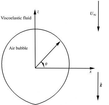
through an incompressible, viscoelastic fluid, as depicted in figure 1. The bubble translates inside an unbounded medium, as in Tsamopoulos et al. (Reference Tsamopoulos, Dimakopoulos, Chatzidai, Karapetsas and Pavlidis2007), in order to eliminate the effects caused by the presence of a confining wall on the flow and stress fields, and, hence, the rise velocity (Herrera-Vélarde et al.
Reference Herrera-Vélarde, Zenit, Chehata and Mena2003). The bubble rises with constant velocity
 $U_{\infty }^{\ast }$
and its material properties, density
 ${\it\rho}_{b}^{\ast }$
, viscosity
 ${\it\mu}_{b}^{\ast }$
, are assumed to be negligibly small with respect to those of the fluid. The interfacial tension
 ${\it\gamma}^{\ast }$
of the gas–liquid interface is assumed constant. Gravity is aligned with, but opposite to the
 $z$
-axis. The chosen reference frame moves with the bubble and the origin of the spherical coordinate system is located at the centre of mass of the bubble. Thus, the bubble remains stationary and the surrounding fluid moves downwards with the opposite velocity
 $U_{f}^{\ast }=-U_{\infty }^{\ast }$
.
Schematic of the flow geometry and coordinate system.

All lengths are scaled with the radius,
 $R_{b}^{\ast }$
, of a spherical bubble with the same volume,
 $R_{b}^{\ast }=(3V_{b}^{\ast }/4{\rm\pi})^{1/3}$
. Since we would like to predict the rise velocity given the remainder of the problem variables, we do not impose it, but scale velocities by balancing buoyancy and viscous forces,
 ${\it\rho}^{\ast }g^{\ast }R_{b}^{\ast 2}/{\it\eta}_{o}^{\ast }$
, where
 $g^{\ast }$
is the gravitational acceleration, and
 ${\it\rho}^{\ast }$
and
 ${\it\eta}_{o}^{\ast }$
are the density and the zero-shear viscosity of the viscoelastic solution, respectively. Similarly, pressure and stresses are scaled by
 ${\it\rho}^{\ast }g^{\ast }R_{b}^{\ast }$
. Hence, the dimensionless numbers that arise are the Archimedes number,
 $Ar={\it\rho}^{\ast 2}g^{\ast }R_{b}^{\ast 3}/{\it\eta}_{o}^{\ast 2}$
, the Bond number
 $Bo={\it\rho}^{\ast }g^{\ast }R_{b}^{\ast 2}/{\it\gamma}^{\ast }$
and the Deborah number
 $De={\it\lambda}^{\ast }{\it\rho}^{\ast }g^{\ast }R_{b}^{\ast }/{\it\eta}_{o}^{\ast }$
. Upon determining the rise velocity, we can use it a posteriori to compute a Deborah number based on it,
 $De_{U}={\it\lambda}^{\ast }U_{\infty }^{\ast }/R_{b}^{\ast }$
, which is related to the previously defined Deborah number via
 $$\begin{eqnarray}De_{U}=U_{\infty }De.\end{eqnarray}$$
This alternative definition of the Deborah number is introduced to facilitate the comparison of the computed rise velocity with the experimental one. When the discontinuity on the rise velocity versus bubble volume occurs,
 $De_{U}$
will also show a discontinuous behaviour with respect to the bubble radius.
2.1. Governing equations
The equations of motion and continuity for an incompressible fluid in dimensionless form are
 $$\begin{eqnarray}\displaystyle & \displaystyle Ar\frac{\text{D}\boldsymbol{u}}{\text{D}t}-\boldsymbol{{\rm\nabla}}\boldsymbol{\cdot }(-P\unicode[STIX]{x1D644}+{\bf\sigma})-\boldsymbol{e}_{z}=\mathbf{0}, & \displaystyle\end{eqnarray}$$
 $$\begin{eqnarray}\displaystyle & \displaystyle \boldsymbol{{\rm\nabla}}\boldsymbol{\cdot }\boldsymbol{u}=0, & \displaystyle\end{eqnarray}$$
 $P$
denotes the isotropic pressure and
 ${\bf\sigma}$
the deviatoric stress tensor. The above system of equations is closed by selecting an appropriate constitutive equation for the deviatoric stress. In the present study, the stress tensor is split into a polymeric and a solvent part as
 $$\begin{eqnarray}{\bf\sigma}={\bf\tau}_{s}+{\bf\tau},\end{eqnarray}$$
where
 $$\begin{eqnarray}{\bf\tau}_{s}=2{\it\beta}\unicode[STIX]{x1D63F}={\it\beta}(\boldsymbol{{\rm\nabla}}\boldsymbol{u}+\boldsymbol{{\rm\nabla}}\boldsymbol{u}^{\text{T}}).\end{eqnarray}$$
In the above equation,
 ${\it\beta}={\it\eta}_{s}^{\ast }/{\it\eta}_{o}^{\ast }={\it\eta}_{s}^{\ast }/({\it\eta}_{s}^{\ast }+{\it\eta}_{p}^{\ast })$
, denotes the ratio of the solvent to the total viscosity, where
 ${\it\eta}_{s}^{\ast }$
denotes the solvent viscosity,
 ${\it\eta}_{p}^{\ast }$
the polymeric viscosity and
 $\unicode[STIX]{x1D63F}$
is the rate-of-deformation tensor. For the polymeric stress components, the exponential Phan-Thien and Tanner constitutive equation (ePTT) is used (Phan-Thien & Tanner Reference Phan-Thien and Tanner1977; Phan-Thien Reference Phan-Thien1978), which is based on polymeric network theory:
 $$\begin{eqnarray}Y({\bf\tau}){\bf\tau}+De\mathop{{\bf\tau}}^{\boldsymbol{{\rm\nabla}}}-2(1-{\it\beta})\unicode[STIX]{x1D63F}=0,\end{eqnarray}$$
where the symbol
 $\boldsymbol{{\rm\nabla}}$
over the viscoelastic stresses denotes the upper convected derivative defined as
 $$\begin{eqnarray}\mathop{\unicode[STIX]{x1D653}}^{\boldsymbol{{\rm\nabla}}}=\frac{\text{D}\unicode[STIX]{x1D653}}{\text{D}t}-(\boldsymbol{{\rm\nabla}}\boldsymbol{u})^{\text{T}}\boldsymbol{\cdot }\unicode[STIX]{x1D653}-\unicode[STIX]{x1D653}\boldsymbol{\cdot }(\boldsymbol{{\rm\nabla}}\;\boldsymbol{u}).\end{eqnarray}$$
For the ePTT model, the function
 $Y({\bf\tau})$
is
 $$\begin{eqnarray}Y({\bf\tau})=\exp \left[\frac{{\it\varepsilon}}{1-{\it\beta}}De\,\mathit{tr}({\bf\tau})\right].\end{eqnarray}$$
The parameter
 ${\it\varepsilon}$
in the function
 $Y({\bf\tau})$
provides a quantitative description of the destruction of the junctions in the viscoelastic network. For
 ${\it\varepsilon}=0$
the Oldroyd-B constitutive model is recovered and its typical values are up to 0.2. When it increases, the shear thinning of the fluid viscosity increases and the extensional viscosity first increases and then decreases (Karapetsas & Tsamopoulos Reference Karapetsas and Tsamopoulos2013).
The above set of equations completes the description of the physical problem when appropriate boundary conditions are applied. To this end, along the free surface of the bubble, the velocity field should satisfy a local force balance between capillary forces, viscous and elastic stresses in the liquid and pressure inside the bubble:
 $$\begin{eqnarray}-\!P\boldsymbol{n}+\boldsymbol{n}\boldsymbol{\cdot }{\bf\sigma}=-P_{b}\boldsymbol{n}+\frac{2H}{Bo}\boldsymbol{n},\end{eqnarray}$$
where
 $P_{b}$
is the pressure inside the bubble,
 $\boldsymbol{n}$
is the outward unit normal to the free surface and
 $2H$
is its mean curvature, which is defined as
 $$\begin{eqnarray}2H=-\boldsymbol{{\rm\nabla}}_{s}\boldsymbol{\cdot }\boldsymbol{n},\quad \boldsymbol{{\rm\nabla}}_{s}=(\unicode[STIX]{x1D644}-\boldsymbol{n}\boldsymbol{n})\boldsymbol{\cdot }\boldsymbol{{\rm\nabla}}.\end{eqnarray}$$
In order to determine the bubble pressure and its rise velocity, which constitutes an essential part in our study, we impose two more equations. To calculate the bubble pressure,
 $P_{b}$
, the dimensionless bubble volume is constrained to remain constant, irrespective of bubble deformation and velocity:
 $$\begin{eqnarray}\int _{s}R_{f}^{3}\sin {\it\theta}\,\text{d}S=2,\end{eqnarray}$$
where
 $R_{f}({\it\theta})$
is the local radial position of the bubble interface. For the calculation of the rise velocity
 $U_{\infty }$
, it is required that the bubble centre of mass remains at the origin of the spherical coordinate system:
 $$\begin{eqnarray}\int _{s}R_{f}^{4}\sin {\it\theta}\cos {\it\theta}\,\text{d}S=0.\end{eqnarray}$$
Finally, on the axis of symmetry (
 ${\it\theta}=0$
and
 ${\it\theta}={\rm\pi}$
) we apply the usual symmetry conditions:
 $$\begin{eqnarray}\displaystyle & \displaystyle u_{{\it\theta}}=0, & \displaystyle\end{eqnarray}$$
 $$\begin{eqnarray}\displaystyle & \displaystyle \frac{\partial u_{r}}{\partial {\it\theta}}=0. & \displaystyle\end{eqnarray}$$
3. Numerical implementation
The mixed finite element method is used for the discretization of velocity, pressure and stress fields combined with an elliptic grid generation scheme advanced by Dimakopoulos & Tsamopoulos (Reference Dimakopoulos and Tsamopoulos2003) for the discretization of the deformed physical domain. With this scheme the physical domain
 $(r,{\it\theta})$
is mapped onto a computational domain
 $({\it\xi},{\it\eta})$
. A computational mesh is generated in the latter domain and the corresponding mesh in the physical domain follows the bubble deformations. As computational domain we choose here the volume that would be occupied by the liquid, if the bubble remained spherical. This mapping is based on the solution of the following system of quasielliptic partial differential equations:
 $$\begin{eqnarray}\displaystyle & \displaystyle \boldsymbol{{\rm\nabla}}\boldsymbol{\cdot }\left\{\left({\it\varepsilon}_{1}\sqrt{\frac{r_{{\it\eta}}+r^{2}{\it\theta}_{{\it\eta}}^{2}}{r_{{\it\xi}}+r^{2}{\it\theta}_{{\it\xi}}^{2}}}+(1-{\it\varepsilon}_{1})\right)\boldsymbol{{\rm\nabla}}{\it\eta}\right\}=0, & \displaystyle\end{eqnarray}$$
 $$\begin{eqnarray}\displaystyle & \displaystyle \boldsymbol{{\rm\nabla}}\boldsymbol{\cdot }\boldsymbol{{\rm\nabla}}{\it\xi}=0, & \displaystyle\end{eqnarray}$$
 ${\it\varepsilon}_{1}$
is a parameter that controls the smoothness of the mapping relative to the degree of orthogonality of the mesh lines. This is adjusted by trial and error; here it is set to 0.1. The boundary conditions for the mesh equations are the same as those used by Tsamopoulos et al. (Reference Tsamopoulos, Dimakopoulos, Chatzidai, Karapetsas and Pavlidis2007) and Dimakopoulos & Tsamopoulos (Reference Dimakopoulos and Tsamopoulos2009).
We approximate the velocity vector as well as the position vector with six-node Lagrangian basis functions,
 ${\it\phi}_{i}$
, and the pressure and stress field with three-node Lagrangian basis functions,
 ${\it\psi}_{i}$
. The weak form of the momentum and continuity equations, along with the numerical implementation of the free surface boundary condition, can be seen in more detail in the work by Tsamopoulos et al. (Reference Tsamopoulos, Dimakopoulos, Chatzidai, Karapetsas and Pavlidis2007). We adapt the EVSS-G method by Brown et al. (Reference Brown, Szady, Northey and Armstrong1993) to solve accurately the governing set of equations, where the polymeric part of the deviatoric stress tensor is split into a purely elastic,
 ${\it\bf\Sigma}$
, and a viscous part:
 $$\begin{eqnarray}{\bf\tau}={\it\bf\Sigma}+2(1-{\it\beta})\unicode[STIX]{x1D63F}.\end{eqnarray}$$
The hyperbolic character of the constitutive equation requires use of the SUPG technique (Brooks & Hughes Reference Brooks and Hughes1982) for its discretization.
In order to determine the complete dependence of the bubble velocity on its volume even in the seemingly discontinuous area, the arclength parameterization of the solution curve is implemented to ensure convergence, when turning points arise during the search for stationary solutions. The value of the physical parameter (e.g. bubble radius, Bond number, etc.), denoted by
 ${\it\mu}$
, becomes an additional component of the vector of all unknown variables,
 $\tilde{\boldsymbol{x}}$
, of the problem, requiring an additional equation for its calculation. For this purpose, given the previous value
 $(\tilde{\boldsymbol{x}}_{o},{\it\mu}_{o})$
of the extended solution vector, its increment,
 $(\tilde{\boldsymbol{x}}-\tilde{\boldsymbol{x}}_{o},{\it\mu}-{\it\mu}_{o})$
is projected on its initial tangent
 $(\partial _{s}\tilde{\boldsymbol{x}}_{o},\partial _{s}{\it\mu}_{o})$
, where the derivatives are taken with respect to the parameter
 $s$
. The product is set equal to the arclength increment
 ${\rm\Delta}s$
, in parameter space, in order to ensure monotonic increase along a solution family. Thus, the following additional equation results:
 $$\begin{eqnarray}F(\tilde{\boldsymbol{x}},{\it\mu},s)=(\tilde{\boldsymbol{x}}-\tilde{\boldsymbol{x}}_{o})\boldsymbol{\cdot }\partial _{s}\tilde{\boldsymbol{x}}_{o}+({\it\mu}-{\it\mu}_{o})\partial _{s}{\it\mu}_{o}-{\rm\Delta}s=0.\end{eqnarray}$$
The unbounded fluid domain is truncated in a way that this inevitable truncation does not affect the numerical approximation of the problem, via the OBC introduced by Papanastasiou et al. (Reference Papanastasiou, Malamataris and Ellwood1992). According to this, far enough from the bubble, at
 $r=R_{\infty }$
, the fluid velocities and stresses are not imposed, but calculated from the weak form of the equations. For example, after applying the divergence theorem, the weak form of the momentum balance becomes
 $$\begin{eqnarray}\int _{{\it\Omega}}[Ar\,\boldsymbol{u}\boldsymbol{\cdot }\boldsymbol{{\rm\nabla}}\boldsymbol{u}{\it\phi}_{i}+\boldsymbol{{\rm\nabla}}{\it\phi}_{i}\boldsymbol{\cdot }{\bf\sigma}+{\it\phi}_{i}\boldsymbol{e}_{z}]\,\text{d}{\it\Omega}-\int _{{\it\Gamma}}[\boldsymbol{n}\boldsymbol{\cdot }{\bf\sigma}]{\it\phi}_{i}\,\text{d}{\it\Gamma}=\mathbf{0},\end{eqnarray}$$
where the term
 $\int _{{\it\Gamma}}[\boldsymbol{n}\boldsymbol{\cdot }{\bf\sigma}]{\it\phi}_{i}\,\text{d}{\it\Gamma}$
is computed according to the OBC method, whereas Dirichlet-type boundary conditions are not imposed. This surface integral term includes the unknown stresses on the flow boundaries. As we will demonstrate shortly (§ 5.1), this procedure is essential for the calculation of the correct stationary solution and the determination of the rise velocity. A rigorous explanation why this treatment of the boundary conditions works is given by Renardy (Reference Renardy1997).
The computational domain is discretized using triangular elements because they conform better to large deformations of the physical domain and can sustain larger distortions than the rectangular ones. Generally, in our simulations a mesh consisting of 100 elements in the radial direction and 100 elements in the azimuthal direction is used, and is properly refined in areas where large stresses are expected. Following the work of Chilcott & Rallison (Reference Chilcott and Rallison1988) and Harlen (Reference Harlen2002), we expect the area of interest to be on the bubble surface and downstream from its south pole along the axis of symmetry, because extended boundary layers of stresses develop there. Thus, following the procedure described in Chatzidai et al. (Reference Chatzidai, Giannousakis, Dimakopoulos and Tsamopoulos2009), a three-level refinement zone is used around the bubble in order to capture accurately the deformations of the bubble interface and the development of intense stress boundary layers, while a two-level refinement zone is introduced at the far-field boundary,
 $R_{\infty }$
, to enhance the accuracy of the calculation of the OBC. All these choices of solution method, OBC, level of discretization, etc. have been checked for numerical convergence. Additionally, our predictions have been critically compared against recent experiments of a bubble rising in rheologically well-characterized viscoelastic fluids by Pilz & Brenn (Reference Pilz and Brenn2007).
4. Fluid rheology
Pilz & Brenn (Reference Pilz and Brenn2007), reported several experiments with rising bubbles in various types of dilute and semidilute viscoelastic fluids. They characterized the fluids they used via rheological diagrams of shear viscosity, storage modulus,
 $G^{\prime }$
, and loss modulus,
 $G^{\prime \prime }$
. According to their observations, a velocity discontinuity is present only for the semidilute solutions, where entanglement effects are present. Thus, we used data from solutions where the discontinuous behaviour on the rise velocity is present, to determine the rheological parameters required in the ePTT constitutive equation:
 ${\it\lambda}^{\ast }$
,
 ${\it\eta}_{o}^{\ast }$
and
 ${\it\varepsilon}$
. To this end, we minimized an objective function containing the deviations between the predicted
 $(G_{fit}^{\prime },G_{fit}^{\prime \prime })$
and measured
 $(G_{exp}^{\prime },G_{exp}^{\prime \prime })$
linear (storage and loss modulus) and simple-shear data:
 $$\begin{eqnarray}\displaystyle C({\it\lambda}_{i}^{\ast },{\it\eta}_{i}^{\ast },{\it\varepsilon})\! & = & \displaystyle \!\mathop{\sum }_{j=1}^{M}\left(\left[\frac{\log (G_{fit}^{\prime }({\it\omega}_{j}))}{\log (G_{exp}^{\prime }({\it\omega}_{j}))}-1\right]^{2}+\left[\frac{\log (G_{fit}^{\prime \prime }({\it\omega}_{j}))}{\log (G_{exp}^{\prime \prime }({\it\omega}_{j}))}-1\right]^{2}\right)\nonumber\\ \displaystyle & & \displaystyle +\,\mathop{\sum }_{l=1}^{L}\left(\left[\frac{\log ({\it\eta}_{fit}(\dot{{\it\gamma}}_{l}))}{\log ({\it\eta}_{exp}(\dot{{\it\gamma}}_{l}))}-1\right]^{2}\right)\!,\end{eqnarray}$$
where
 $M$
and
 $L$
are the total number of angular frequencies and shear rates read from their experimental diagrams, which typically are 30 and 20, respectively. The present objective function differs from that given in Bird, Armstrong & Hassager (Reference Bird, Armstrong and Hassager1987), by using the logarithmic function on the calculated and measured rheological values. The reason for this choice is to describe more accurately the rheological parameters in both small and large deformation rates, and consequently to predict more accurately the rise velocity of the bubble. For the exponential Phan-Thien & Tanner model, the values of
 $G^{\prime }$
, and
 $G^{\prime \prime }$
, in the limit of small amplitude oscillatory flow
 ${\it\delta}\ll 1$
, where
 ${\it\delta}$
denotes the amplitude of the oscillation, are the same as those derived using the multimode upper convected Maxwell (UCM) model (Phan-Thien & Tanner Reference Phan-Thien and Tanner1977; Phan-Thien Reference Phan-Thien1978; Bird et al.
Reference Bird, Armstrong and Hassager1987),
 $$\begin{eqnarray}G_{fit}^{\prime }({\it\omega}_{j})=\mathop{\sum }_{k=1}^{N}\frac{{\it\eta}_{k}{\it\lambda}_{k}{\it\omega}_{j}^{2}}{1+({\it\lambda}_{k}{\it\omega}_{j})^{2}},\quad G_{fit}^{\prime \prime }({\it\omega}_{j})=\mathop{\sum }_{k=1}^{N}\frac{{\it\eta}_{k}{\it\omega}_{j}}{1+({\it\lambda}_{k}{\it\omega}_{j})^{2}}.\end{eqnarray}$$
These expressions do not depend on the value of
 ${\it\varepsilon}$
and, hence, its determination from the linear viscoelastic properties of the fluid is not possible. Thus, in order to extract the
 ${\it\varepsilon}$
parameter, the third term in the objective function is added, which accounts for the deviations from the experimentally measured shear viscosity, which is affected by this parameter. For the simple-shear experimental data, the reduced constitutive equation for the shear stress is
 $$\begin{eqnarray}{\it\tau}_{xy,i}^{\ast }\exp \left({\it\varepsilon}\left(\frac{{\it\lambda}^{\ast }}{{\it\eta}_{o}^{\ast }}{\it\tau}_{xy,i}^{\ast }\right)^{2}\right)=2{\it\eta}_{o}^{\ast }\dot{{\it\gamma}}_{i}^{\ast }.\end{eqnarray}$$
Solving (4.3) with
 ${\it\tau}_{xy,i}^{\ast }$
as the unknown for specific
 $\dot{{\it\gamma}}_{i}^{\ast }$
by using a root-finding method, e.g. bisection, we calculate the value of shear viscosity via the following formula:
 $$\begin{eqnarray}{\it\eta}_{fit}^{\ast }(\dot{{\it\gamma}}_{i}^{\ast })=\frac{{\it\tau}_{xy,i}^{\ast }}{\dot{{\it\gamma}}_{i}^{\ast }}.\end{eqnarray}$$
The relaxation time,
 ${\it\lambda}^{\ast }$
, and zero-shear viscosity,
 ${\it\eta}_{o}^{\ast }$
, used in (4.3) have been obtained as follows:
 $$\begin{eqnarray}{\it\lambda}^{\ast }=\frac{\displaystyle \mathop{\sum }_{i=1}^{N}{\it\lambda}_{i}^{\ast }{\it\eta}_{i}^{\ast }}{\displaystyle \mathop{\sum }_{i=1}^{N}{\it\eta}_{i}^{\ast }},\quad {\it\eta}_{o}^{\ast }=\mathop{\sum }_{i}^{N}{\it\eta}_{i}^{\ast }.\end{eqnarray}$$
In order to predict more accurately the exact fluid behaviour exploiting the entire spectra of their properties during the numerical calculations, the fluids have been approximated as a four-node network during the fitting progress. Hence, the minimization of
 $C$
is achieved iteratively as follows: values of
 ${\it\lambda}_{i}^{\ast },{\it\eta}_{i}^{\ast },i=1,\ldots ,4$
, and
 ${\it\varepsilon}$
are assumed,
 $G_{fit}^{\prime }$
and
 $G_{fit}^{\prime \prime }$
are computed via (4.2) with
 $N=4$
for different
 ${\it\omega}_{j}$
, then
 ${\it\eta}_{fit}^{\ast }$
is computed via (4.4) for different
 ${\it\gamma}_{i}^{\ast }$
, and finally the cost function (4.1) is computed. The optimal set of
 ${\it\lambda}_{i}^{\ast },{\it\eta}_{i}^{\ast },i=1,\ldots ,4$
, and
 ${\it\varepsilon}$
is used to produce the predicted steady shear viscosity, storage and loss modulus as a function of shear rate,
 $\dot{{\it\gamma}}^{\ast }$
, and angular frequency,
 ${\it\omega}$
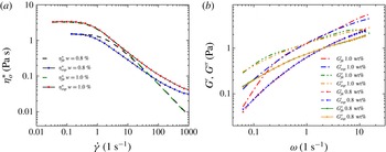
, respectively. These curves are compared in figure 2 with the experimental ones for data corresponding to Praestol 2500 (a linear poly-acrylamide) at concentrations 0.8 and 1.0 wt%. The extracted rheological parameters are listed in table 1.
(a) Simple-shear data,
 ${\it\eta}_{o}^{\ast }$
versus
 $\dot{{\it\gamma}}$
, (b) linear oscillatory shear measurements,
 $G^{\prime }$
,
 $G^{\prime \prime }$
versus
 ${\it\omega}$
.

Linear and nonlinear viscoelastic properties for P2500 at
 $w=0.8\,\%$
and
 $w=1.0\,\%$
obtained upon nonlinear fitting to the ePTT constitutive model.

5. Results and discussion
5.1. Validation of the open-boundary condition
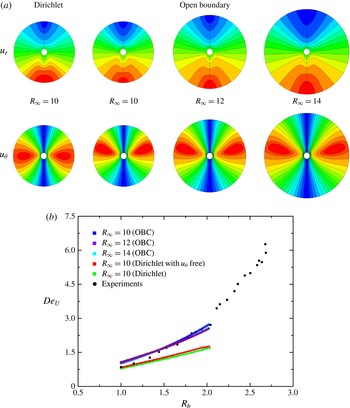
The employment of the OBC in the far-field boundary facilitates the correct description of the physics in the unbounded flow case and, thus, helps in eliminating any spurious effects on the flow field that could be induced by either the presence of a wall or arbitrary Dirichlet conditions, especially when elastic effects extend to long distances from the bubble (Herrera-Vélarde et al. (Reference Herrera-Vélarde, Zenit, Chehata and Mena2003) and Pillapakkam et al. (2008)). To ensure the validity and the efficacy of the OBC on bubble dynamics, tests varying the location of the far-field boundary,
 $R_{\infty }$
, have been performed based on the case of P2500,
 $w=0.8\,\%$
. Contour plots for the radial,
 $u_{r}$
, and azimuthal,
 $u_{{\it\theta}}$
, velocity components are illustrated in figure 3(a) for three different values of
 $R_{\infty }$
, namely
 $10,12,14$
. Henceforth, the ratio
 $$\begin{eqnarray}R_{b}=R_{b}^{\ast }/R_{bo}^{\ast }\end{eqnarray}$$
(a) Convergence of the results for the velocity components with increasing
 $R_{\infty }$
corresponding to
 $(R_{b},Ar,De,Bo)=(1.97,0.018,4.8,0.34)$
and
 ${\it\varepsilon}=0.05$
for P2500 0.8 wt%. (b) Direct comparison of OBC with different
 $R_{\infty }$
and DBC with experimental data for P2500 0.8 wt%.

is defined as the independent variable when comparison between the calculated and the experimental rise velocity is discussed. Here,
 $R_{b}^{\ast }$
denotes each experimentally measured bubble radius and
 $R_{bo}^{\ast }$
corresponds to the radius of the smallest bubble available in each experimental curve of Pilz & Brenn (Reference Pilz and Brenn2007) for a specific polymeric solution. In the present comparison,
 $R_{b}=1.97$
for P2500,
 $w=0.8\,\%$
. No differences can be observed between the results of the contour lines of the velocity components, even in the far-field region. The three plots of contour lines match perfectly up to the
 $R_{\infty }$
value, for which each one has been computed. Certainly, as
 $R_{\infty }$
increases, the mesh needed to obtain mesh-independent results is refined accordingly. For example, for
 $R_{\infty }=10$
, 25 000 elements are required, while for
 $R_{\infty }=14$
, the element number needs to be increased to 40 000. From now on, all reported results have been obtained using the optimal combination of
 $R_{\infty }$
and mesh density, which is
 $R_{\infty }=10$
and a total of 25 000 triangular elements. Comparing the computed flow fields with OBC with those obtained using the Dirichlet boundary condition (DBC) (figure 3
a), we observe even qualitative differences on the locations where
 $u_{{\it\theta}}$
obtains its maximum value, for example. The flow field seems to be ‘trapped’ in a sphere with radius
 $R_{\infty }$
, which through the DBC imposes an artificial symmetry plane on
 $u_{{\it\theta}}$
at the bubble equator. This observation concurs with the report of Sigli & Coutanceau (Reference Sigli and Coutanceau1977), who analysed the steady fall of a sphere in a UCM fluid using DBC at the far field. For a fixed reference frame, they predicted secondary flow fields downstream of the sphere as the Weissenberg number increases, a result which is in contrast to several experimental and numerical works, which do not observe the negative wake for fluids without shear thinning. Additionally, comparing the computed rise velocity (figure 3
b), using DBC at the far field with the one computed using the OBC for the same polymeric solution, reveals the essential contribution of the unbounded fluid assumption on the physics of the problem. While the results obtained with the OBC, with different
 $R_{\infty }$
, follow accurately the experimentally measured values of the Deborah number based on the rise velocity, those with DBC fail to predict the value of rise velocity even for bubbles with only twice as large a radius as the smallest one. Finally, in cases where elasticity is high, large extensional stresses are expected to be present, which may extend even beyond the computational outflow boundary. Obviously, the use of the DBC will affect the values of the developed viscoelastic stresses, because it will impose on
 $R_{\infty }$
the undisturbed flow field. Hence, the use of the OBC is essential for the correct prediction of the rise velocity and, consequently, for the accurate simulation of the whole phenomenon.
5.2. Overall comparison with previous experimental results
The predictions of the present work have been compared with the measurements by Pilz & Brenn (Reference Pilz and Brenn2007), who reproduced experimentally the discontinuity in the rise velocity versus bubble volume diagrams. They used a container with a height approximately 4 times the side of its square cross-section and this, in turn, was at least 20 and 120 times larger than the diameter of the larger and smaller, respectively, bubble that we will be able to compare our results with theirs. This eliminates any three-dimensional disturbances that could be induced by the proximity of the wall (You et al.
Reference You, Borhan and Haj-Hariri2009) or effects of wall-modified elastic stresses on the magnitude of the rise velocity (Herrera-Vélarde et al.
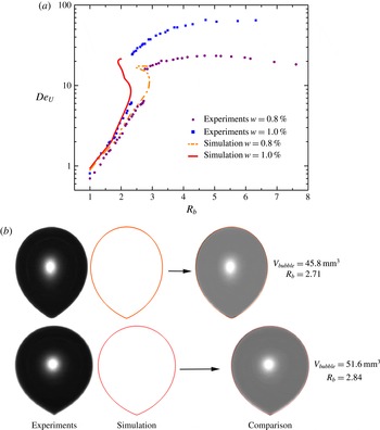
Reference Herrera-Vélarde, Zenit, Chehata and Mena2003). In figure 4(a) the experimental and predicted values of the velocity-based Deborah number for P2500,
 $w=0.8\,\%$
and
 $w=1.0\,\%$
, are shown. The exact reproduction of the experimental values of the bubble rise velocity is obvious in both cases. In figure 4(a), we observe that the stationary solutions for the rise velocity can be split into three branches. According to bifurcation theory (Seydel Reference Seydel1994), the branches with the lower and larger velocity-based Deborah number are stable, while the middle branch between the two turning points is unstable. The critical bubble radius, where the discontinuity occurs, is the bubble radius for which the slope of the curve becomes infinite. In each hysteresis loop the existence of two limit points gives rise to two such critical values. The first limit point corresponds to the lower stable branch when the radius increases and the second limit point to the upper stable branch when the radius decreases. In each case, moving slightly past the limit point, the solution will ‘jump’ to the other branch. For the solution with
 $w=0.8\,\%$
of P2500 we find the first critical value is just under
 $R_{b}=2.91$
, when the jump occurs from the lower to the upper branch, and the second critical value is approximately
 $R_{b}=2.45$
, when the opposite occurs. Computations for the solution with
 $w=1.0\,\%$
of P2500 reveal that the first critical radius is approximately
 $R_{b}=2.31$
and the second critical radius is approximately
 $R_{b}=1.9$
. Clearly there is a range of bubble radii for which both stable solution branches coexist. Given that in all experimental studies we are aware of, the bubble radius was increased, it is more likely that the critical values reported and depicted in their plots correspond to a jump from the lower to the upper branch. So, in the first experiment, the critical bubble radius is
 ${\sim}$
2.72 and in the second one is
 ${\sim}$
2.33, in very good agreement with our predicted values.
(a) Comparison of our predictions for the Deborah number based on the rise velocity versus normalized bubble radius, in polymeric solutions P2500 0.8 and 1.0 wt%. (b) Shapes of air bubbles in an aqueous 0.8 wt% P2500 solution compared to our predictions below (top,
 $V=45.8~\text{mm}^{3}$
) and above (bottom,
 $V=51.6~\text{mm}^{3}$
) the critical bubble volume.

Numerical difficulties arose when we tried to continue on the upper branch of the solution family to higher velocities or, equivalently, higher
 $De_{U}$
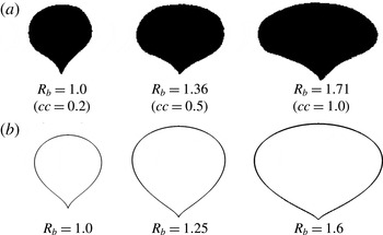
numbers. We conjecture that this is caused by either the known difficulty to compute at higher dimensionless elasticity, possibly because of the development of sharper stress boundary layers or the existence of three-dimensional solutions, which cannot be captured with our two-dimensional axisymmetric analysis. Additionally, our computations succeed in reproducing accurately the bubble shapes that we obtain from the experiments. The experimental bubble shapes shown in figure 7 of Pilz & Brenn (Reference Pilz and Brenn2007) for P2500,
 $w=0.8\,\%$
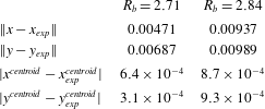
, are reproduced in grey scale, our corresponding predictions are given with the red lines and, as shown in the last column of figure 4(b), the two shapes superimpose perfectly. The first row of shapes are for a bubble radius below the critical value for the ‘velocity jump’, while the second row are for a bubble radius above the critical value. The overall shapes of the two bubbles are only slightly different. Their clearer difference is in the downstream pole, where the tip is more distinct in the larger bubble. Further from the qualitative comparison of the bubble shapes, we followed the same technique described by Fraggedakis et al. (Reference Fraggedakis, Kouris, Dimakopoulos and Tsamopoulos2015) to compare quantitatively the computed results with the experimental ones. To this end, we computed the Euclidean norms of the differences between published experiments and our predictions in each bubble shape and the centroids of the bubbles, which are presented in table 2. The norms have been computed by simply adding the contributions from 200 equidistributed points on bubble surfaces. The (not normalized) norms are below 0.01 and the errors in the centroids below 0.001. Clearly, for the first time, and without any fitting parameters, we have achieved quantitative agreement with the experiments using an axisymmetric steady analysis.
Euclidean norms of the deviation between the shapes and the centroid location computed via our calculations and those found in the experiments by Pilz & Brenn (Reference Pilz and Brenn2007).

5.3. Physical interpretation of the experimental results
First, we will present our analysis of the
 $w=0.8\,\%$
solution of P2500, where our computations succeed in capturing the experimental data, including a significant portion of the upper branch of stationary solutions. The continuation procedure is based on slowly changing the dimensionless bubble radius. This parameter affects all dimensionless numbers,
 $Ar$
,
 $Bo$
and
 $De$
, that arise in the present study. Thus, effectively, a multiparameter arclength continuation is being carried out, simultaneously increasing all three dimensionless numbers, although
 $Ar$
never exceeds
 $10^{-3}$
in these experiments. In figure 4(a), we observe two regions where the rise velocity exhibits hysteresis. This is something that has not been reported in any experimental studies, where only a single large ‘jump’ is present in the rise velocity magnitude versus bubble volume.
5.3.1. First hysteresis loop: formation of bubble tip and negative wake
In the first hysteresis loop, the changes in the rise velocity are negligible (only
 ${\sim}$
25 % increase) and, thus, it was undetectable in experiments containing even shear-thinning fluids (Pilz & Brenn Reference Pilz and Brenn2007). As we will describe and explain below, the numerical computations reveal the appearance of the so-called negative wake, reported in previous works with air bubbles, and the formation of a tip in the rear pole of the bubble (Hassager Reference Hassager1979; Herrera-Vélarde et al.
Reference Herrera-Vélarde, Zenit, Chehata and Mena2003).
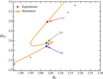
Figure 5 shows in more detail the two turning points that divide the locus of steady-state solutions into three branches. It is important to note here that excessive mesh refinement has been performed to ensure the accuracy of the computations and the existence of these turning points. Increasing the number of refinement levels by factor of two around the bubble surface, the results remain unchanged and retain a qualitative differentiation before and after the velocity discontinuity. We have chosen to discuss the qualitative differences between three steady solutions for identical bubble radius
 $(R_{b}=2.03)$
. In the following figures the blue and red lines correspond to the stable solutions with the lower and higher rise velocities, respectively, while the green line corresponds to the unstable solution. The most significant changes occur on the bubble surface and along the axis of symmetry downstream from the bubble.
First hysteresis loop enlarged. Deborah number based on the rise velocity versus normalized bubble radius. Three cases are considered for
 $(R_{b},Ar,De,Bo)=(2.03,0.019,4.95,0.35)$
.

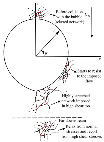
Figure 6 depicts the deformation of entangled macromolecules (depicted as a network only for visualization purposes) as it translates around the stationary bubble. First, the macromolecules are squeezed on the upstream pole of the bubble and undergo biaxial extension, but the zero-shear condition there and along the bubble surface allows them to translate almost freely around it and up to the equatorial plane. The building up of the elastic stresses intensifies for
 ${\it\theta}\approx 3{\rm\pi}/4$
, leading to maximum stretching of the chains at the downstream pole at
 ${\it\theta}={\rm\pi}$
, which pulls the bubble surface, thus producing the tip. A similar qualitative picture (their figure 19) has been described by Pilz & Brenn (Reference Pilz and Brenn2007). The chains try to resist this deformation, developing a shear layer. Moving downstream away from the bubble, the chain extension starts to relax. The normal stresses relax faster than the shear stresses, generating a velocity which points away from the bubble pole. The reason for this behaviour is that the extensional viscosity reaches its upper bound before shear thinning starts to be pronounced behind the bubble. This is clearly seen in figure 9 of the work by Karapetsas & Tsamopoulos (Reference Karapetsas and Tsamopoulos2013). This is the mechanism leading to the negative wake. In contrast, in the case of a sphere sedimenting in a viscoelastic medium, Arigo et al. (Reference Arigo, Rajagopalan, Shapley and McKinley1995) and Harlen (Reference Harlen2002) have shown that the larger shear stresses form this shear layer earlier at
 ${\it\theta}\approx 3{\rm\pi}/4$
, while the stagnation point flow necessitates that the normal stresses are small and are maximized further downstream.
Sketch of polymeric network travelling along the bubble surface.

For clarity, variables on the bubble surface will be shown with respect to the azimuthal direction
 $({\it\theta}^{\circ })$
. Considering that the stress tensor is related to the conformation tensor via Kramers’ relation (Tsouka et al.
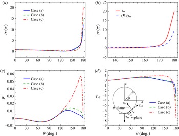
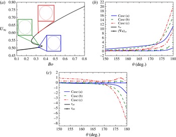
Reference Tsouka, Dimakopoulos, Mavrantzas and Tsamopoulos2014), it can be said that its trace corresponds to the degree to which the viscoelastic medium has been stretched (Chilcott & Rallison Reference Chilcott and Rallison1988). When network elements reach the rear pole of the bubble, their instant configuration becomes highly stretched (birefringent pipe, Malaga & Rallison (Reference Malaga and Rallison2007)), see figure 7(a). The forces there develop a ‘birefringent strand’ region (Harlen, Rallison & Chilcott Reference Harlen, Rallison and Chilcott1990), where both
 $(\boldsymbol{{\rm\nabla}}u)_{rr}$
and
 ${\it\tau}_{rr}$
, see figure 7(b), indicate that extended polymers lie on the outgoing streamline near the rear pole (Noh et al.
Reference Noh, Kang and Gary Leal1993; Malaga & Rallison Reference Malaga and Rallison2007; You et al.
Reference You, Borhan and Haj-Hariri2009). Noh et al. (Reference Noh, Kang and Gary Leal1993) argued that uniaxial straining flow (large
 $(\boldsymbol{{\rm\nabla}}u)_{rr}$
for
 ${\it\theta}^{\circ }\in (165,180)$
, see figure 7(b)) is primarily responsible for stretching the medium at the rear pole, leading finally to the change of bubble shape from spherical (first stable solution) to an egg-like shape (second stable solution). Nevertheless, they were not able to predict a cusp-shaped tip due to convergence difficulties with their numerical scheme, which imposed strict orthogonality on the mesh (Ryskin & Leal Reference Ryskin and Leal1984). The elliptic grid generation used in the present work (Dimakopoulos & Tsamopoulos Reference Dimakopoulos and Tsamopoulos2003), combined with the finer mesh on the bubble surface and on the axis of symmetry, allows us to predict highly deformed interfaces, even when a cusp is formed (Papaioannou et al.
Reference Papaioannou, Giannousakis, Dimakopoulos and Tsamopoulos2014).
(a) Trace of stress tensor, (b)
 ${\it\tau}_{rr}$
and
 $(\boldsymbol{{\rm\nabla}}u)_{rr}$
, (c) radial velocity, (d) shear stresses
 ${\it\tau}_{r{\it\theta}}$
on the bubble surface. Three cases correspond to
 $(R_{b},Ar,De,Bo)=(2.03,0.019,4.95,0.35)$
.

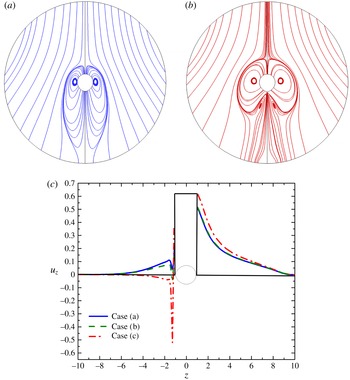
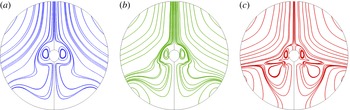
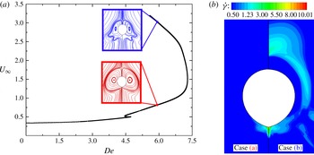
The radial velocity in the lower (case a) and middle (the unstable case b) branches remains small around the bubble and returns to zero at its downstream pole. Hence this remains a stagnation point for the flow. In contrast, on the upper branch (case c), it increases after the equatorial plane and remains positive on the downstream pole (figure 7
c). Hence, the stagnation point flow has turned into a converging flow locally at the tip. The elimination of the stagnation point has been previously observed in experiments where laser-Doppler velocimetry was used to measure the velocity magnitude upstream and downstream from air bubbles along the axis of symmetry (Hassager Reference Hassager1979; Bisgaard Reference Bisgaard1983) and anticipated by Chilcott & Rallison (Reference Chilcott and Rallison1988). The deformed bubble shape favours the development of shear stresses on it for all three solutions because the tangential vector on the surface no longer coincides with
 $\boldsymbol{e}_{{\it\theta}}$
. This becomes clearer when the tangential stress balance is considered
 $$\begin{eqnarray}\boldsymbol{t}\boldsymbol{\cdot }[{\bf\sigma}\boldsymbol{\cdot }\boldsymbol{n}]=0\Rightarrow t_{r}(n_{r}{\it\sigma}_{rr}+n_{{\it\theta}}{\it\sigma}_{r{\it\theta}})+t_{{\it\theta}}(n_{r}{\it\sigma}_{r{\it\theta}}+n_{{\it\theta}}{\it\sigma}_{{\it\theta}{\it\theta}})=0,\end{eqnarray}$$
while near the tip
 $\boldsymbol{n}\neq \boldsymbol{e}_{r}$
and
 $\boldsymbol{t}\neq \boldsymbol{e}_{{\it\theta}}$
. Hence, although the tangential stress is zero,
 ${\it\tau}_{r{\it\theta}}$
is not. In fact, the shear stress on the bubble surface is rather small and positive (i.e. slightly hindering the bubble rise) up to
 ${\it\theta}\approx 120^{\circ }$
, but becomes very large and negative for larger angles, attaining a maximum value at the downstream pole. In these areas, a large-magnitude elastic shear stress develops (figure 7
d), creating a net force which ‘pushes’ the air bubble in the upward direction because of the negative sign of
 ${\it\tau}_{r{\it\theta}}$
, especially at the tip. This net force is responsible for the creation of the hysteresis loop, because now the bubble is forced to translate faster inside the viscoelastic medium. It should be recalled here that the main contribution to stress stems from material elasticity, while the contribution of viscous forces due to the solvent is negligible. This means that dissipative terms are of a little importance. Chilcott & Rallison (Reference Chilcott and Rallison1988) have mentioned that a shearing region may exist in the ‘cusp’ region, a fact that is revealed in the present work. The large shear stress, which exists at
 ${\it\theta}={\rm\pi}$
, starts to relax as fluid elements travel on the axis of symmetry and their magnitude decays to zero after approximately one dimensionless radius.
(a,b) Flow field around the bubble before (blue) and after (red) the velocity jump. (c) Axial velocity along the axis of symmetry, the bubble axis is in
 $-1<Z<1$
. Three cases are considered for
 $(R_{b},Ar,De,Bo)=(2.03,0.019,4.95,0.35)$
.

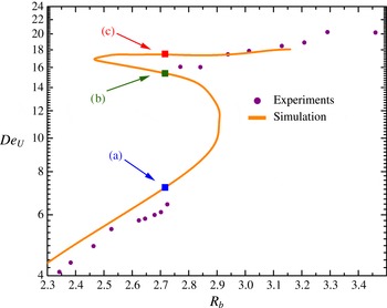
Second hysteresis loop enlarged. Deborah number based on the rise velocity versus normalized bubble radius. Three cases correspond to
 $(R_{b},Ar,De,Bo)=(2.71,0.047,6.62,0.63)$
.

The negative shear stress, which has developed near the lower part of the south hemisphere of the bubble, gives rise to elastic recoil (Bird et al. Reference Bird, Armstrong and Hassager1987) and the fluid elements are forced to rotate (Arigo & McKinley Reference Arigo and McKinley1998), creating a second and smaller toroidal ring of streamlines downstream from the bubble, see figure 8(a,b) (case c), whereas a single toroidal ring exists in the lower branch (case a). The transformation of the rear pole into a tip favours the creation of an extended shear region downstream of the air obstacle and leads to the formation of the negative wake structure along and near the axis of symmetry (figure 8 c). Thus the flow elements follow more complex patterns downstream of the bubble in the second stable solution, although their effect on the bubble shape is rather small. Harlen (Reference Harlen2002) found that the negative wake is eliminated when solid boundaries are translated away from the particle. In the present study, despite the fact that we account for an unbounded fluid, negative velocities downstream of the axis of symmetry are observed. In the bubble case, shear layers near and on the surface develop due to the tip formation (Chilcott & Rallison Reference Chilcott and Rallison1988) and not due to the existence of solid boundaries near the obstacle, as in the motion of a rigid particle (Lunsmann et al. Reference Lunsmann, Genieser, Armstrong and Brown1993; Arigo et al. Reference Arigo, Rajagopalan, Shapley and McKinley1995). In contrast to previous experimental observations (Herrera-Vélarde et al. Reference Herrera-Vélarde, Zenit, Chehata and Mena2003) the negative wake along the axis of symmetry arises here before the second hysteresis loop, which we will discuss in the next section. Therefore, the complete change in the flow field, reported by experimentalists after the ‘large’ velocity jump, should be separated from the ‘negative wake’ and the tip formation. Nevertheless, in the second hysteresis loop both the ‘negative wake’ and the tip are intensified.
5.3.2. Second hysteresis loop (the so-called velocity jump)
The second hysteresis loop predicted in the present calculations is illustrated in figure 9. Now a much larger increase in the magnitude of the rise velocity occurs,
 ${\sim}$
250 %. As in the previous section, we concentrate on three different steady solutions for identical radii
 $(R_{b}=2.73)$
. In comparison with the previously predicted hysteresis, the flow field variables and stresses on the surface and along the axis of symmetry downstream of the air obstacle do not show any qualitative changes as the continuation tracks the solution family. Additionally, the observations during the first hysteresis are valid here too, meaning that the quantities on the surface and the axis of symmetry have the same behaviour, but with slightly larger values.
The entangled polymer chains in these regions are subjected to the same extensional straining flow as before, which leads us to believe that the reason for the second discontinuity of the rise velocity versus bubble volume should stem from information at the bulk of the fluid around the air obstacle. It is interesting to emphasize that Malaga & Rallison (Reference Malaga and Rallison2007), in their calculations, have only included the free surface of the bubble and modelled the presence of the birefringent strand. Hence, one of the reasons that they could not reproduce the velocity jump may be missing information concerning the flow rearrangement and its effect on the fluid properties in the bulk region and near the bubble. On the other hand, despite considering the entire flow field in their calculations and predicting the velocity discontinuity, the transient level set method of Pillapakkam et al. (Reference Pillapakkam, Singh, Blackmore and Aubry2007) did not resolve the interface and the stresses there accurately enough to explain the qualitative differences that occur during the change of stationary solutions along the solution family. Also, the container they used was small compared with the bubble radii, and hence interactions between elastic stresses and the wall were introduced. Perhaps for this reason, their results exhibited intense secondary flow fields similar to those observed in the negative wake, a result that contradicts the predictions by Harlen (Reference Harlen2002), who states that the negative wake cannot be present in models with unbounded elongational viscosity, e.g. the Oldroyd-B model. These arguments lead us to believe that the secondary flow field they observed is due to the bubble–wall interaction.
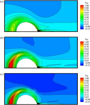
 ${\it\tau}_{{\it\theta}{\it\theta}}$
stresses along the second hysteresis loop,
 $(R_{b},Ar,De,Bo)=(2.71,0.047,6.62,0.63)$
. (a) Case (a), (b) case (b), (c) case (c).

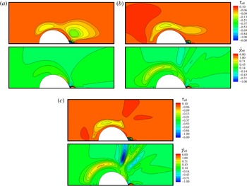
 ${\it\tau}_{r{\it\theta}}$
stress and
 $\dot{{\it\gamma}}_{r{\it\theta}}$
along the second hysteresis loop,
 $(R_{b},Ar,De,Bo)=(2.71,0.047,6.62,0.63)$
. (a) Case (a), (b) case (b), (c) case (c).

The trace of the stress tensor is overwhelmed by the large values of
 ${\it\tau}_{rr}$
near the free surface and at the rear pole and cannot characterize the qualitative changes that occur in the bulk region upstream and downstream of the bubble. In contrast, when the second velocity jump has already taken place, it is predicted that the maximum
 ${\it\tau}_{{\it\theta}{\it\theta}}$
in front of the bubble is doubled in comparison to its maximum value before the jump, enhancing the biaxial extensional flow near the front stagnation point (figure 10). We should mention that the flow direction is from left to right, while the bubble remains stationary with its centre at the origin of the spherical coordinates. The impact of this stress increase on the velocity field is projected on the
 $\dot{{\it\gamma}}_{r{\it\theta}}$
component of the deformation tensor (figure 11). Before the occurrence of the discontinuity, its variation is limited only at the lower hemisphere of the bubble. When the solution lies on the upper branch of the curve,
 $\dot{{\it\gamma}}_{r{\it\theta}}$
also increases in the region where biaxial straining flow is intense (case (c) in figure 11). Hence, the shear viscosity characteristics of the fluid cause a local decrease in the viscosity in front of the bubble (Herrera-Vélarde et al.
Reference Herrera-Vélarde, Zenit, Chehata and Mena2003). Combining the reduced resistance at the front of the bubble with the presence of the intense shear layer at the rear pole, the created net force produced by the negative
 ${\it\tau}_{r{\it\theta}}$
pushes more effectively on the air obstacle, facilitating its faster movement inside the viscoelastic medium.
Flow field variations around the air bubble during the second hysteresis loop for
 $(R_{b},Ar,De,Bo)=(2.71,0.047,6.62,0.63)$
. (a) Case (a), (b) case (b), (c) case (c).

Close-up of streamlines, including applied forces on certain control volumes around the bubble, for case (c) of figure 12. The length of the stress components is proportional to their magnitude.

In the previous section, describing the first hysteresis loop, we showed that the negative wake was generated by the interplay between
 ${\it\tau}_{r{\it\theta}}$
and
 ${\it\tau}_{rr}$
, while shear stresses apply an upward force on the bubble. In the lower branch of the second hysteresis loop
 ${\it\tau}_{r{\it\theta}}$
remains important, but not so in the upper branch, where the shear stress near the lower hemisphere is no longer high (case (c) in figure 11). The role of the shear force in the negative wake formation, which also tends to rotate the fluid particles, is undertaken by
 ${\it\tau}_{{\it\theta}{\it\theta}}$
(case (c) in figure 10). In regions slightly far away from the bubble surface and approximately at
 ${\it\theta}\approx 3{\rm\pi}/4$
,
 ${\it\tau}_{{\it\theta}{\it\theta}}$
has a negative value, creating the corresponding net force which produces the secondary flow field downstream the bubble (case (c) in figure 12). It is noteworthy that, before the second velocity jump (cases (a,b) in figure 12), the created recirculation observed at the first hysteresis has now been eliminated because shear stresses relax faster than the extensional stresses. Once more, from figures 10–12 we observe that the bubble shape has changed very little before and after the velocity jump. The dramatic change in the velocity field after the second velocity discontinuity has been observed by Herrera-Vélarde et al. (Reference Herrera-Vélarde, Zenit, Chehata and Mena2003) and predicted by Pillapakkam et al. (Reference Pillapakkam, Singh, Blackmore and Aubry2007), who found, however, that the centre of the secondary flow field is closer to the free surface, in contrast to our predictions. We believe that this happens because of the proximity of their bubble to the wall.
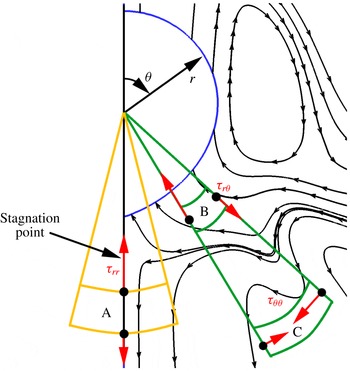
A close up view of the bubble and the streamlines from figure 12 case (c) is given in figure 13. Here the predicted stress field has been added in the fluid and around three control volumes (CV), the first one of which includes the axis of symmetry. The flow stagnation point, which indicates the initiation of the negative wake, is also given. The total
 ${\it\tau}_{rr}$
stress component in CV-A pulls the fluid towards the bubble, the
 ${\it\tau}_{r{\it\theta}}$
component shown in CV-B pushes the bubble upwards, while the
 ${\it\tau}_{{\it\theta}{\it\theta}}$
component shown in CV-C forces the fluid to rotate in the counter-clockwise direction.
5.3.3. Single hysteresis loop with P2500,
 $w=1.0\,\%$
(all three phenomena appear together)

In this experiment a single hysteresis loop arises. It should be noticed that the critical normalized radius is smaller than the previous case, although the dimensional radius is slightly larger (
 $R_{b}^{\ast }=2.3~\text{mm}$
here versus
 $R_{b}^{\ast }=2.2~\text{mm}$
in the second hysteresis loop of the previous case). The value of
 ${\it\varepsilon}$
in the PTT model, resulting from fitting the rheological data (table 1), is larger, indicating the more pronounced shear-thinning behaviour of this more concentrated solution of P2500. Again, we examine thoroughly three different stationary solutions for the same normalized radius,
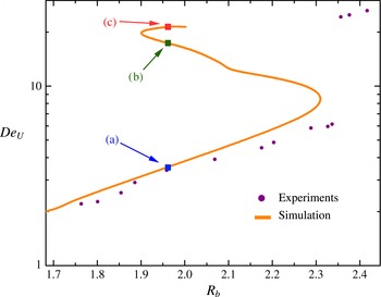
 $R_{b}=1.96$
(figure 14). The bubble rise velocity on the upper branch is 6.3 times larger than that in the lower branch. In all experiments, with a variety of polymeric solutions, a single discontinuity has been reported, with the velocity rising by a factor from 3 to 10 compared to its value before the critical volume.
Hysteresis enlarged for Praestol P2500,
 $w=1.0\,\%$
. Deborah number based on the rise velocity versus normalized bubble radius. Three cases are considered for
 $(R_{b},Ar,De,Bo)=(1.96,0.01,8.94,0.55)$
.

(a) Mean curvature, (b) trace of the polymeric stress tensor, (c) shear stress
 ${\it\tau}_{r{\it\theta}}$
on the bubble surface, and (d) shear rate
 $\dot{{\it\gamma}}$
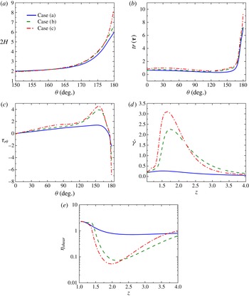
and (e) shear viscosity on the axis of symmetry at the front of the bubble. Three cases correspond to
 $(R_{b},Ar,De,Bo)=(1.96,0.01,8.94,0.55)$
.

Here, when the solution lies on the lower (stable) branch, only large extensional stresses are developed and the area of their action is restrained to only 3–4 radii from the bubble rear pole. Moreover, the negative wake does not appear and the downstream pole of the bubble is deformed, but a clear tip is not present. In contrast, on the upper branch, the mean curvature at the rear pole increases abruptly (figure 15 a). Whereas the dimensionless curvature for a spherical surface is 2, its increases to 6 in the rear pole of the lower branch and 8.5 in the rear pole of the upper branch. This is a consequence of the large extensional stresses that are developed there (figure 15 b). The change of the shape at the rear pole enhances the development of intense shear layers further, facilitating the formation of a tip (figure 15 c). The forces caused by the large shear are the same as those discussed in the first hysteresis loop of the previous sections (§§ 5.3.1–5.3.2), but in the present case they develop at the same time as the velocity jump. For the steady state on the upper branch, the extensional stresses extend up to the outflow boundary, which means that they extend more than 10 radii away from the bubble rear pole. The usage of the OBC is again proved to be essential for the smooth relaxation of the viscoelastic stresses up to the edge of the computational domain without the introduction of numerical errors in general, and particularly in the rise velocity. When the tip is formed, a converging flow field is established at the rear pole and the stagnation point is eliminated (Hassager Reference Hassager1979; Bisgaard Reference Bisgaard1983). For the upper stable solution, the forces generated by the shear layer are responsible for the larger acceleration of the bubble. They result in larger fluid displacement and, hence, a stronger biaxial straining flow at the front of the bubble. This is obvious from figure 15(d), where the variation of shear rate on the axis of symmetry at the front of the bubble is illustrated. A little above the bubble front, an increase in the strain rate is observed, which is maximized only half a radius away. This results in the minimization of the shear viscosity in the same location (figure 15 e). It is noteworthy that the minimum value of the viscosity is approximately 10 times smaller than its value at the bubble surface. Therefore, the developed stresses at the rear pole push the bubble upwards more effectively, because the viscosity at the front region is decreased, resulting in the larger increase of the rise velocity and, thus, to the so-called velocity jump.
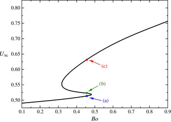
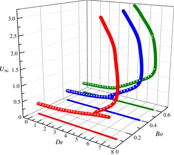
Rise velocity for varying Bond number and
 $(Ar,De,{\it\varepsilon},{\it\beta})=(0,5,0.01,10^{-4})$
.

5.3.4. On the Boger fluid limit
$({\it\varepsilon}\rightarrow 0)$

Next we will approach the conditions for a Boger-type fluid by reducing the value of
 ${\it\varepsilon}$
of the PTT model as much as possible. These fluids are characterized by pronounced elastic effects, while their shear viscosity remains constant during deformation. This parameter controls the shear-thinning and the elongational behaviour of the fluid (see, for example, Pavlidis, Dimakopoulos & Tsamopoulos (Reference Pavlidis, Dimakopoulos and Tsamopoulos2009), Karapetsas & Tsamopoulos (Reference Karapetsas and Tsamopoulos2013)). Using such a small
 ${\it\varepsilon}=0.01$
and solvent ratio,
 ${\it\beta}=10^{-4}$
, numerical difficulties arise during the continuation in the normalized bubble radius, so we choose a constant value for
 $De=5$
and, hence,
 $Bo$
remains the only continuation parameter. On the new hysteresis loop three cases are considered again for the identical value of
 $Bo=0.46$
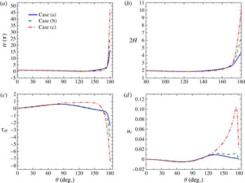
(figure 16). When the solution lies on the lower branch, the bubble has a prolate shape and its rear pole tends to form a tip. In contrast with the previously discussed cases, the maximum value of the elongational viscosity is larger, and hence larger values of elongational stresses are developed at the rear pole (figure 17
a). These are responsible for the change of the mean curvature, because stronger forces pull out the rear pole. The value of the mean curvature in these regions is almost three times larger than in the case before the abrupt increase on the rise velocity (figure 17
b), and the bubble rear pole is transformed clearly into a tip. The change of shape of the bubble bottom favours the development of negative shear stress (figure 17
c), which pushes the bubble in the upward direction. When the stagnation flow is eliminated in the rear of the bubble, the radial velocity is no longer zero (figure 17
d).
(a) Trace of stress tensor, (b) mean curvature,
 $2H$
, (c) shear stress
 ${\it\tau}_{r{\it\theta}}$
and (d) radial velocity
 $u_{r}$
on the bubble surface. Three cases correspond to
 $(Ar,De,{\it\varepsilon},{\it\beta})=(0,5,0.01,10^{-4})$
.

Considering the previous predictions, one may wonder why the tip formation is not followed always by the negative wake. The decoupling of these two phenomena has been observed in experiments involving Boger fluids (figure 3 in Vélez-Cordero et al. (Reference Vélez-Cordero, Sámano and Zenit2012)). In cases where
 ${\it\varepsilon}\rightarrow 0$
, we find that large extensional stresses,
 ${\it\tau}_{rr}$
, are developed at the rear pole of the bubble, creating a pointed tip region. These forces are extended far downstream from the bubble surface. As a consequence, this uniaxial straining, combined with the converging flow due to the shape of rear pole, decreases the residence time of polymers in regions near the gas obstacle. The created shear layer now relaxes faster in space than the extensional forces, and hence the force which rotates the fluid elements is no longer able to create the negative wake structure. Instead, the so-called ‘extended wake’ is developed (Arigo & McKinley Reference Arigo and McKinley1998), reaching the downstream outflow boundary. Moreover, the observed velocity discontinuity in Boger fluids (Vélez-Cordero et al.
Reference Vélez-Cordero, Sámano and Zenit2012) is smaller in magnitude than in experiments where shear-thinning effects are present (Astarita & Apuzzo Reference Astarita and Apuzzo1965; Leal et al.
Reference Leal, Skoog and Acrivos1971; Liu et al.
Reference Liu, Liao and Joseph1995; Herrera-Vélarde et al.
Reference Herrera-Vélarde, Zenit, Chehata and Mena2003). The reason for this is the lack of reduction in the flow resistance, as discussed in §§ 5.3.2 and 5.3.3. Interestingly, the ratio of velocities after and before the predicted hysteresis in figure 16 equals 1.25, which is close to the value of 1.3 observed by (Vélez-Cordero et al.
Reference Vélez-Cordero, Sámano and Zenit2012).
Finally, Kopf-Sill & Homsy (Reference Kopf-Sill and Homsy1987) studied the bubble motion in a Hele-Shaw cell. Despite the fact that their working fluid was Newtonian, they observed bubbles with long tails when the flow rate increased. These shapes were accompanied by a discontinuity on the rise velocity of the bubble, which increased by 40 %. We conjecture that a similar mechanism may be responsible for the discontinuity in their work, as an extended shear layer could have developed on its rear surface, where a tip-like shape arises.
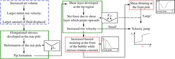
Schematic representation of the event sequence leading to the velocity jump. The blue box assigns the events that are valid in Newtonian fluids also, the green box the events that are present both in Boger and shear-thinning fluids, while the red box correspond to the events that are present in shear-thinning fluids only.

5.3.5. Proposed mechanism for the velocity jump
Figure 18 presents a summary of the mechanism leading to the so-called ‘velocity jump’. The box with blue and discontinuous outline includes the effects seen in Newtonian liquids as well, the boxes with green continuous outline show the effects that are present in Boger and shear-thinning fluids, while the boxes in red dotted outline show the effects that are present in shear-thinning fluids only. As the bubble volume increases, the displaced amount of fluid increases too and the bubble tends to move initially with a larger rise velocity. This produces larger strains in the polymer, which is squeezed upon the bubble front and then moves around it. The residence time of the polymer on the bubble surface is smaller than its relaxation time and, hence, it will start resisting the imposed deformation downstream from its equator. Consequently, large extensional elastic stresses (Ramaswamy & Leal Reference Ramaswamy and Leal1999) develop at the rear pole region and affect the bubble shape significantly. They pull the bubble rear pole and change its shape from spherical to a teardrop-like shape. This shape favours the development of a shear layer which opposes the flow in the vicinity of the tip. Hence, a net force which acts on the tip area is developed and points in the upward direction, facilitating bubble movement. Beyond a critical force level, the biaxial straining flow at its front region becomes intense and enhances changes in the properties of the medium. In particular, the viscosity of the host fluid is decreased ahead of the bubble, while the effect of the shear forces at the tip increases. In conclusion, the combined effect of buoyancy and the produced net force ‘kick’ the bubble, producing the discontinuity in its velocity.
A question that naturally arises is why the velocity versus volume discontinuity occurs only in bubbles and not in rigid particles. First of all, the extensional forces which act on the free surface favour the tip formation only in the case of a bubble. The tip shape allows the development of forces which act at the bottom of the bubble and point in the direction it moves. It is commonly accepted that, when a tip is formed, an abrupt increase in the velocity of the bubble takes place (Leal et al.
Reference Leal, Skoog and Acrivos1971; Liu et al.
Reference Liu, Liao and Joseph1995; Herrera-Vélarde et al.
Reference Herrera-Vélarde, Zenit, Chehata and Mena2003). In rigid particles, the forces generated by its movement are concentrated on its surface approximately at
 ${\it\theta}\approx 3{\rm\pi}/4$
(Lunsmann et al.
Reference Lunsmann, Genieser, Armstrong and Brown1993; Arigo et al.
Reference Arigo, Rajagopalan, Shapley and McKinley1995; Harlen Reference Harlen2002). These forces are always present in the same area on its surface. Additionally, the effect of a force which acts on a rigid particle is not the same as would act on a particle with a much smaller density, say a balloon. Therefore, the combination of the deformability of its surface with the rheological fluid properties produces the velocity discontinuity, while the velocity of a sedimenting sphere increases monotonically with its volume.
5.4. Parametric analysis
As already mentioned, increasing the bubble radius affects all three dimensionless numbers. It is interesting to examine separately the effects of fluid elasticity and interfacial tension on bubble dynamics. Moreover, we will restrict ourselves to
 $Ar=0$
, as its largest value that could arise in experiments is 0.1 (Herrera-Vélarde et al.
Reference Herrera-Vélarde, Zenit, Chehata and Mena2003; Soto et al.
Reference Soto, Goujon, Zenit and Manero2006; Vélez-Cordero et al.
Reference Vélez-Cordero, Sámano and Zenit2012), even for the largest bubbles studied. Also, the Reynolds number does not exceed 0.1 for materials where bubble rise velocity shows the discontinuous behaviour.
5.4.1. Surface tension effects – continuation on
$Bo$

Based on the experimental observations of Pilz & Brenn (Reference Pilz and Brenn2007), we kept the same
 ${\it\varepsilon}=0.05$
and
 ${\it\beta}=6.6\times 10^{-4}$
for these calculations. In the following results the bubble radius, fluid density and the Deborah number remain constant, while changes in the Bond number are caused by changes in the surface tension.
Rise velocity versus Bond number, for different fixed Deborah numbers and
 $({\it\varepsilon},{\it\beta})=(0.05,6.6\times 10^{-4})$
.

Figure 19 summarizes the solution families generated for different Deborah numbers. For liquids where elasticity is not high,
 $De=3$
, the rise velocity increases monotonically with decreasing surface tension, in agreement with Malaga & Rallison (Reference Malaga and Rallison2007) and You et al. (Reference You, Borhan and Haj-Hariri2009). For moderate elasticity,
 $De=4$
, a sharp increase in velocity appears, but a hysteresis loop is not present yet. The developed extensional stresses at the rear pole of the bubble are larger in magnitude than before, turning the spherical bubble into an egg-like shape, but without eliminating the rear stagnation point. For
 $De>4$
, the evolution of the rise velocity with respect to the Bond number exhibits a hysteresis loop and a converging flow at the tip area is established (Chilcott & Rallison Reference Chilcott and Rallison1988). The critical Bond number where the discontinuity is present decreases with increasing Deborah number, and the magnitudes of elongational stresses developed at the rear pole of the bubble are increased. Thus, they are able to overcome earlier the surface tension locally and, hence, deformation of the free surface proceeds in order to balance the forces on the bubble surface. Additionally, the magnitude of the velocity jump increases too, because elasticity favours the development of larger shear stresses at the tip region; thus the effective force which kicks the bubble to move faster inside the medium is larger.
In order to demonstrate the above observations, we discuss further the case of
 $De=5$
. The increase of the rise velocity versus
 $Bo$
is illustrated in figure 20(a). Three cases are considered in the hysteresis loop for the same Bond number,
 $Bo=0.32$
, to make clearer what happens before (blue) and after (red) the velocity jump. In the same figure we present the corresponding bubble shapes. When the jump takes place, a small tip develops due to the intense extensional straining flow in this area (figure 20
b), producing a highly stretched network. Hence, large extensional stresses are developed which deform the bubble surface (Chilcott & Rallison Reference Chilcott and Rallison1988; Noh et al.
Reference Noh, Kang and Gary Leal1993; Malaga & Rallison Reference Malaga and Rallison2007). The tangential vector on the free surface does not coincide with
 $\boldsymbol{e}_{{\it\theta}}$
, allowing a shear layer, which opposes the imposed stretching (figure 20
c). Also, a force which is attributed to the increase of
 ${\it\tau}_{{\it\theta}{\it\theta}}$
, squeezes the lower hemisphere of the bubble near its tip, leading finally to the experimentally observed egg-like shape. For moderate elasticity numbers,
 $De\sim 5$
, the velocity jump is accompanied by the negative wake, the mechanism of which has been discussed already.
(a) Rise velocity for varying Bond number and
 $(Ar,De,{\it\varepsilon},{\it\beta})=(0,5,0.05,6.6\times 10^{-4})$
, (b)
 ${\it\tau}_{rr}$
stresses (lines without symbols) and
 $(\boldsymbol{{\rm\nabla}}u)_{rr}$
(lines with triangle symbols), (c)
 ${\it\tau}_{r{\it\theta}}$
(lines without symbols) and
 ${\it\tau}_{{\it\theta}{\it\theta}}$
(lines with triangle symbols) stresses on bubble surface for
 ${\it\theta}^{\circ }\in (150,180)$
along the hysteresis for
 $Bo=0.32$
.

When hysteresis is predicted, the increase in the rise velocity does not exceed 30 %. The reason why the velocity jump is not as sharp as in the experiments lies in the local properties of the fluid at the front of the bubble. By keeping its elasticity constant and decreasing the surface tension, the stress at the front of the bubble does not increase as in the case discussed in § 5.3.2. There, all the physical parameters depending on the bubble radius were changing simultaneously, allowing the increase of viscoelastic stresses and the decrease in the viscosity of the host fluid (figure 11). Instead, here the magnitude of the jump velocity is closer to that observed in Boger fluids by Vélez-Cordero et al. (Reference Vélez-Cordero, Sámano and Zenit2012).
5.4.2. Elasticity effects – continuation on
$De$

Next we examine changes of the fluid elasticity only by changing
 $De$
. The evolution of the rise velocity in parameter space is shown in figure 21. Each curve corresponds to a different
 $Bo$
. In contrast with the previous section, the velocity jump is always present for all
 $Bo$
we used. Unfortunately, the computations break down when the rise velocity exceeds approximately 3, leaving the upper branch after the large velocity jump undetermined. Maybe the two-dimensional axisymmetric analysis is not sufficient to predict these solutions and a three-dimensional flow field around the bubble may exist. Despite the fact that we are not able to predict the upper branch curve, the rise velocity variation shows the same qualitative behaviour as has been observed in experiments involving shear-thinning fluids (Astarita & Apuzzo Reference Astarita and Apuzzo1965; Leal et al.
Reference Leal, Skoog and Acrivos1971; Zana & Leal Reference Zana and Leal1977; Liu et al.
Reference Liu, Liao and Joseph1995; Herrera-Vélarde et al.
Reference Herrera-Vélarde, Zenit, Chehata and Mena2003; Soto et al.
Reference Soto, Goujon, Zenit and Manero2006; Pillapakkam et al.
Reference Pillapakkam, Singh, Blackmore and Aubry2007; Pilz & Brenn Reference Pilz and Brenn2007). When surface tension is large, e.g.
 $Bo\leqslant 0.5$
, two hysteresis loops seem to be present, a result in agreement with the predictions of § 5.3 for the 0.8 % solution of P2500. The hysteresis which corresponds to the small velocity jump is followed by change in the bubble shape. During the large-magnitude hysteresis, fluid properties around the front section of the bubble change, facilitating the faster movement of the bubble. To examine more specifically these observations, we consider the case where
 $Bo=0.4$
, the solution curve of which can be seen in figure 22(a). The small hysteresis has been extensively described in § 5.3.1, so our interest here lies in the solutions with the large variations of the rise velocity. Two cases are considered for the same
 $De=6$
. The flow field corresponding to the solution of the lower branch is similar to that obtained right before the velocity jump using the multiparameter analysis in § 5.3.1. Along the unstable branch, significant changes in the flow field occur affecting the shear rate around the bubble (figure 22
b). An area with larger shear rate is developed a little ahead of the upper hemisphere of the bubble and is responsible for the local change of the rheological properties of the fluid. When the solution lies on the unstable branch, the bubble encounters a less viscous fluid and is able to move faster through it. Additionally, in correspondence with the bubble radius continuation, the area where shear stresses act downstream of the bubble starts to shrink and a larger
 ${\it\tau}_{{\it\theta}{\it\theta}}$
stress develops. Along the unstable branch, there is a switch between the forces which are responsible for the negative wake formation, with
 ${\it\tau}_{{\it\theta}{\it\theta}}$
now being the main stress component, which causes rotation of the fluid elements. Furthermore, the abrupt increase in the rise velocity imposes on the surrounding medium a stronger elongational flow, biaxial ahead of and uniaxial behind the bubble, which is responsible for the highly stretched polymer chains around its free surface and far downstream of its rear pole.
Rise velocity versus Deborah number, for different fixed Bond numbers.

(a) Rise velocity for varying Deborah number and
 $(Ar,Bo,{\it\varepsilon},{\it\beta})=(0,0.4,0.05,10^{-4})$
, (b) shear rate,
 $\Vert \dot{{\bf\gamma}}\Vert$
for
 $De=6$
along the hysteresis region.

5.5. Comparison with experiments including inertia
The large impact of inertia on the bubble shapes as
 $Re/Ar$
increases has been observed experimentally (Astarita & Apuzzo Reference Astarita and Apuzzo1965; Soto et al.
Reference Soto, Goujon, Zenit and Manero2006) and theoretically (Noh et al.
Reference Noh, Kang and Gary Leal1993). It is widely known in Newtonian fluids (Tsamopoulos et al.
Reference Tsamopoulos, Dimakopoulos, Chatzidai, Karapetsas and Pavlidis2007) and non-Newtonian fluids that inertia is responsible for flattening the upper hemisphere of the bubble forming spherical cap shapes. Without having the exact rheological characterization and properties of the fluids used by Astarita & Apuzzo (Reference Astarita and Apuzzo1965), it is not possible to replicate their reported bubble shapes for quite large values of
 $Ar$
,
 $Bo$
and
 $De$
, e.g. for their commercial polymer solution named J-100. Considering fluids with
 ${\it\beta}=0.1$
and
 ${\it\varepsilon}=0.05$
, tests have been conducted to find the most appropriate set of parameters where similar shapes could be reproduced. Although the fluid rheology is not known, we succeeded in predicting bubble shapes similar to the last three in the first row of figure 5 from their work (figure 23). Table 3 summarizes the parameter values for these bubble shapes.
Experimental versus predicted bubble shapes for J-100, Astarita & Apuzzo (Reference Astarita and Apuzzo1965) under the conditions given in table 3. (a) Experiments, (b) simulation.

Values of dimensionless numbers for the bubble shapes predicted in figure 23.

Inertia affects the biaxial straining flow significantly at the front stagnation point, causing the upper hemisphere to be flattened, creating an oblate-spheroid bubble with a tip (right bubble), because of fluid elasticity. Also, when surface tension is weakened, the extensional straining flow that exists due to high elasticity favours the formation of a cusp.
6. Conclusions
We have carried out an extensive investigation of bubble dynamics rising through a viscoelastic liquid when the bubble radius increases. Experimental evidence (Astarita & Apuzzo Reference Astarita and Apuzzo1965; Pilz & Brenn Reference Pilz and Brenn2007) reveals a sharp increase in the rise velocity of the bubble when its volume reaches a critical value and the discontinuous behaviour in the related diagrams is depicted by two separate branches of solution families. So far in the literature, this phenomenon has been called ‘velocity jump’. In the present work, via pseudo arclength continuation, we were able to connect the two seemingly separate solution branches through a hysteresis loop and accurately predict the critical volume observed in experiments by Pilz & Brenn (Reference Pilz and Brenn2007). Additionally, in less shear-thinning fluids and at a smaller bubble radius than the critical value, a smaller in magnitude velocity jump is predicted. The smaller hysteresis loop is found to be linked with the bubble shape deformation and the formation of the so-called negative wake, Hassager (Reference Hassager1979). Along the hysterisis loop, the bubble rear pole is transformed into a tip, allowing the establishment of a converging flow field locally at this region and eliminating the rear stagnation point of the bubble. Also, the local change of curvature results in the development of an intense shear layer and the formation of a net force which points upwards. This force allows the bubble to move faster, resulting in the slightly increased rise velocity. The second hysteresis loop is accompanied by changes in the shear rates in front of the bubble. Hence, the rheological properties of the fluid change; especially the shear viscosity is decreased. The reduced shear viscosity lowers the resistance to flow, and thus the net force from the intense shear stress at the rear pole acts more effectively on the free surface, abruptly increasing the rise velocity of the bubble. The mechanism which leads to the formation of the negative wake structure is found to change during the second hysteresis loop. Before the critical volume and after the first predicted hysteresis, the developed shear stress downstream of the bubble is responsible for its creation (Harlen Reference Harlen2002). After the second velocity jump, the shear stress is replaced by a larger
 ${\it\tau}_{{\it\theta}{\it\theta}}$
stress. This now acts in the same way as the shear stress on the fluid, but forms larger and more extensive secondary flows below the equator and near the surface of the bubble. The above results are in agreement with the study by Herrera-Vélarde et al. (Reference Herrera-Vélarde, Zenit, Chehata and Mena2003). When the shear thinning of the fluid is stronger, the two hysteresis loops merge into one, and the tip and negative wake formation occur simultaneously with the large velocity jump.
Separate continuation analysis is performed on the dimensionless numbers of
 $De$
and
 $Bo$
to distinguish the effects of elasticity and capillarity. During
 $Bo$
continuation,
 $De$
remains fixed. Here a single hysteresis loop is predicted with a relatively smaller velocity jump. Thus, the inability of the surface tension to balance the extensional stress is responsible for the transformation of the rear pole into a tip and, consequently, for the formation of a shear layer which pushes the bubble to move faster. Only during
 $De$
continuation do two hysteresis loops appear to be present. By increasing
 $De$
, the polymeric stresses around the bubble are increased too, resulting in a decrease of the shear viscosity around bubble surface. This effect is possible only when shear thinning is taken into account and it is not a coincidence that the sharp and large increase in the rise velocity is present only in experiments involving shear-thinning fluids. On the other hand, in Boger-type fluids, the velocity jump is much smaller in magnitude (Vélez-Cordero et al.
Reference Vélez-Cordero, Sámano and Zenit2012).
Finally, we extended our computations to predict shapes of larger bubbles when both inertia and elasticity are present. Although exact rheological data have not been reported for the corresponding experiments, we obtained qualitative agreement with the bubble shapes reported by Astarita & Apuzzo (Reference Astarita and Apuzzo1965).
Acknowledgements
This work has been supported financially by the General Secretariat of Research and Technology of Greece through the programme ‘Thales’ via the project entitled ‘COVISCO’ and the European project entitled ‘MIFIS-Internal flow simulations’. Additionally, we are grateful to Professor Brenn for sharing with us his rheological data.