The paper by Lundborg, Nystedt & Lindgren (Reference Lundborg, Nystedt and Lindgren2007) offered an interesting contribution to the growing literature on marriage markets, which mostly builds on Gary Becker's seminal work (Reference Becker1981). In contrast to the previous literature, Lundborg et al. (Reference Lundborg, Nystedt and Lindgren2007) utilize the BMI as a proxy to evaluate the extent to which people in Europe are governed by the risk of experiencing divorce when shaping their physical appearances. The multiple regression models of Lundborg et al. (Reference Lundborg, Nystedt and Lindgren2007) estimated via ordinary least squares (OLS) showed some evidence for the thesis that married people in societies where divorce risks, proxied by the national divorce rates, are high are more inclined to invest in their outward appearance. Lundborg et al. (Reference Lundborg, Nystedt and Lindgren2007) proved that divorce risks among married individuals are negatively connected to BMI but unrelated among singles. High divorce rates, they concluded, make people prepare for a potential divorce and future return to the marriage market.

The attempt to reproduce and verify the findings of Lundborg et al. (Reference Lundborg, Nystedt and Lindgren2007) has led to the detection of some problems in estimation and to emergence of quite different results. In particular, there is a major flaw in the analysis of Lundborg et al. (Reference Lundborg, Nystedt and Lindgren2007), related to the application of OLS to hierarchal structured data. The primary problem in estimating the effect of the national divorce rate on the individual BMI by OLS results from the fact that BMI varies among persons but the divorce rate only varies among the context units, namely countries. This circumstance is often ignored in traditional analysis, but violates assumptions of OLS regression. The principal problem arises from the standard errors of the regression coefficients of context variables. Their estimation depends on the sample size (Verbeek, Reference Verbeek2003, p. 22). Yet, the use of context variables in OLS results in their disaggregation and causes a distinct underestimation of the standard errors. Hence the significance of the independent variables is systematically overrated (Hans, Reference Hans2006, p. 7). The disposition of the multilevel analysis is not plagued with these issues and solves them. Multilevel models are designed to deal with two or more levels and permit simultaneous analysis. Additionally, multilevel modelling allows determination of the explained variance at each level and of the totalized explained variance.

The following part describes the general process of multilevel modelling applied to the analysis of Lundborg et al. (Reference Lundborg, Nystedt and Lindgren2007). The described analysis is performed for all sub-samples (singles and married persons). The starting point for a multilevel analysis is the formulation of a fully unconditional model, without any predictors. The aim here is to determine the variance distribution between the individual and the country level. Regarding the question of Lundborg et al. (Reference Lundborg, Nystedt and Lindgren2007), the unconditional model has the following form, known as Random Intercept Only (RIO):

(1)

The BMI of an individual i living in country j is characterized by constant β ₀ for all countries, a random effect u _0j, and the error term e_ij. The random effect varies between the observed countries. The error term refers to dissimilarities between the persons. The total variance consists of the sum of the variation of the regression constant Σu _0j² and the sum of the variation of the error term Σe_ij ². Now the proportion of the country-specific variance in the total variance, which is also named the intra-class correlation coefficient ρ, can be analysed.

(2)

By means of Equation (2) it is possible to determine how much variance of the common variance is due to differences between the countries, and thereby the proportion of the total variance that can be explained by country variables (i.e. the divorce rate). For the determination of the effect of the independent variables an additional model is needed, which is denoted as Random Intercept (RI). This model contains accessorily the independent variables of the individual and the country level. The equation is as follows:

(3)

The significance of the individual-level variables is calculated analogously to OLS models, since the coefficients are approximately t-distributed with n–(p+q)−1 degrees of freedom, where n is the number of observations, and p+q is the number of independent variables at individual and country level. By contrast, the coefficient of country variables is t-distributed too, but with N–q–1 degrees of freedom, where N is the number of countries (Hans, Reference Hans2006, p. 23). Because the variance is separated into two levels, two different methods of measurement are needed to determine the explained variance at each level. The approach of Raudenbush & Bryk (Reference Raudenbush and Bryk2002, p. 74) is applied here, since the inclusion of individual-level variables reduces the error variance at this level. The percentage of reduction can be determined by the difference between the error variance at individual level (var_RIO(e_ij)) in the RIO model and the (reduced) error variance at individual level in the RI model (var_RI(e_ij)) divided by the error variance at individual level (var_RIO(e_ij)) in the RIO model.

(4)

The explained variance at the country level follows this equation:

(5)

As with the individual-level calculation the reduction of the variance component is used, but now the variance components at country level are utilized. The procedure is depicted in Equation (5) by var_RI–IV(u _0j) for the error variance in an RI model, which only contains predictors at the individual level, and var_RI(u _0j) for the error variance in the full RI model (both individual and country variables).

(6)

A measure for the goodness-of-fit of the full RI model is the Maddala Pseudo-R ² (Equation 6), which is based on the differences in the deviance between the RIO model and the RI model. The calculations were performed with SAS 9.1 using PROC MIXED and restricted maximum likelihood (REML).

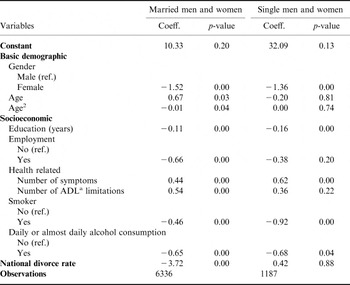
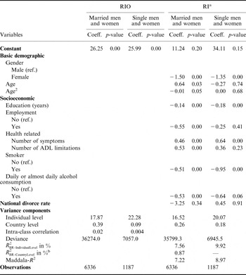
Table 1 reports the estimations via OLS analogous to Lundborg et al. (Reference Lundborg, Nystedt and Lindgren2007). The figures suggest an effect of the national divorce risk on BMI for married persons, but not for singles. The reproduction of this result should prove that this analysis is using the same baseline data. Despite careful preparation of data, there remain minor differences between the reproduced figures and the original ones. Table 2 presents the estimations via the applied linear multilevel model. The first two columns show the RIO models, which give information on the distribution of variance by individual and country components. The variance of the country component is very low compared with the individual level. The country-specific variance of the total variance is 2% for married people and 0.4% for singles (see intra-class correlation), which can be explained by country variables. Columns 3 and 4 show the Random Intercept models with the independent variables (individual and country levels). There is no significant effect of the national divorce rate on BMI for either married people or singles. Moreover, the insignificant variable only explains 0.87% of country-specific variance among married people. For singles, there is no explanatory content of the divorce rate. The Maddala-R ² as a measure of goodness-of-fit represents 7.22% and 8.97% of the total variance for married people and singles respectively. This outcome is almost solely caused by the explanatory content of the individual variables.

Table 1.

Parameter estimates via OLS on BMI

^a ADL: activities of daily living.

Table 2.

Parameter estimates via linear multilevel models on BMI

^a Random Intercept model with individual and country variables.

^b The Random Intercept models with individual variables only for the calculation of the R ² are not reported.

In conclusion, this re-analysis revealed that there is no significant connection between BMI and divorce risk among married people. Therefore the findings of Lundborg et al. (Reference Lundborg, Nystedt and Lindgren2007) are questioned, since the previous results are apparently the product of an inadequate statistical method. Furthermore, there is hardly any explanatory content on the country level. The country level seems not to be the proper unit of analysis. A more regional viewpoint is indicated. As for textual improvement suggestions, in general, the body shape of singles is also central to the decision to reduce body weight if married people prepare for a future return to the marriage market. Only if singles have a lower BMI will there be an incentive for the married to slim. Consequently, the BMIs of the married also have to be compared with those of singles. This should be considered in further investigations.