I. Introduction
Many studies produce data consisting of rankings or ratings of n objects by m judges. Almost every award and admission to a competitive program is based on such data. In this paper, we are concerned with measuring the quality of rankings and ratings specifically for the judging of wines. Because both rankings and ratings are typically produced using the assessments of two or more judges, their consistency is one measure of the quality of the resulting ranking or rating. We discuss advantages and disadvantages of a variety of measures that have been or could be used for evaluating wine judge consistency.
Ranking means that the objects are arranged in order of some attribute, from largest to smallest or vice versa. Rating means that objects are sorted into categories with similarly defined attributes. Rankings and ratings are usually based on an underlying score assigned by a judge or judges. The scores can be interval, meaning that the differences in scores are comparable, or ordinal, in which case they are not. Whether the score is interval or ordinal, and whether ranking or rating is the goal, determines the data analysis needed to assess consistency of judging.
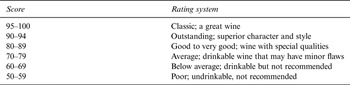
The scoring systems for ranking or rating wines may assign numbers between 80 and 100 or employ a 100-point scale; scores are regarded as ordinal rather than numerical. The scoring of wine quality depends on many factors: aesthetics, pleasure, complexity, color, appearance, odor, aroma, bouquet, tartness, and the interactions with the senses of these characteristics. Table 1 illustrates the wine-rating system employed by a well-known wine journal, Wine Spectator. Other wine journals have different rating systems: a summary of such systems can be found at www.wine.com. It is notable that so many variables have been condensed to such a gross scoring system. Many studies examining the judging of wine have found consistency to be lower than desired (Cao and Stokes, Reference Cao and Stokes2010; Gawel and Godden, Reference Gawel and Godden2008; Hodgson, Reference Hodgson2008, Reference Hodgson2009). The multifactor nature of scoring may explain this lack of consistency. However, inconsistency may compromise the credibility of wine competitions and thereby lead to a loss of consumer confidence in the competition results.
Example of Wine-Rating System

Neither rankings nor ratings are meaningful unless there is a minimum level of consistency (or concordance) among judges. A maximum ranking consistency ignores the closeness of the scores and occurs when all judges rank the wines in the same order. It can be achieved even if the judges do not have perfectly consistent rankings but requires the additional condition that judges' assigned scores are close enough that they fall in the same category. If a set of judges produces rankings that are independent of one another, then the ranks provide no information of the merits of the wines. An exception to this occurs if information on the relative competency of the judges is available or can be discerned from the rankings themselves.
Measuring the consistency of ratings has been studied in different disciplines for decades, and there is a long bibliography on methods. Some of the key descriptive terms that apply are: methods of concordance, measures of agreement, multirater data, ranking methods, interrater reliability, paired comparisons, and rater agreement (or judge agreement). Judge agreement, which we use as a generic term, can refer to exact matching for nominal ratings or consistency of the ranking. There is little consensus about which statistical methods are best for measuring judge agreement.
The goal of this paper is to describe a variety of those methods and what they can be used for, to describe explicitly what they measure, and to provide guidance on their proper usage in analyzing wine-tasting data. Wine tasting is a popular event for both the specialist and the general public. For example, the website (www.liquidasset.com) created and maintained by Orley Ashenfelter and Richard Quandt provides rich wine-tasting data, wine-tasting analyses, and articles. We single out several papers that provide statistical analyses that relate to the current tutorial. Some of the discussions overlap with our paper, so we suggest that these papers be viewed as complementary to the current paper (Ashenfelter and Quandt, Reference Ashenfelter and Quandt1999; Ginsburgh and Zang, Reference Ginsburgh and Zang2012; Quandt, Reference Quandt2007). Specifically, Quandt (Reference Quandt2006) published a paper in the Journal of Wine Economics titled “Measurement and Inference in Wine Tasting.” The author discussed three topics: (1) testing ranking of wines in blind tastings, (2) evaluating judge agreement, and (3) testing how well judges identify the wines. In doing so, he provided a valuable introduction of statistical methods on these topics. Quandt used Kendall's coefficient of concordance to measure judge agreement. Our contribution in the paper is describing and comparing a number of measures of judge agreement in different scenarios (i.e., two judges, more than two judges, wine tastings across years). By doing this, we hope to provide more depth on measuring and testing judge agreement in wine tasting.
The methods we review range from simple to complex and from familiar to new. In general, there is a tradeoff between simplicity of the measure and richness of the information about wine judging that it provides. In some cases, a simple method that provides information about a single feature of the scoring is best; in other cases, a need to distinguish more detail about the scoring process calls for a more complex method.
In this paper, assume that the goal for judge consistency is that the order of rankings or ratings agrees. We first review the simplest case of two judges and n wines (Section II) to fix ideas and then generalize to m > 2 judges and n wines (Section III), which is the usual situation. These analyses provide measures of judge consistency within one study. However, tasting of the same wines may take place at different localities or across different years. For the analyses of these data, we provide a survey of methods to compare judge agreement over multiple datasets (Section IV). In Section V, we discuss a number of analyses other than judge agreement, which includes comparing two specific wines evaluated by m judges, the method of paired comparisons that generates a network, and the design of a wine-tasting event using a balanced incomplete block design.
II. Analysis for Two Judges and n Wines
The simplest wine-tasting event is the case in which two judges each taste n wines and provide a score. The scoring can be a numerical value (discussed in Section II.A) or a rank (discussed in Sections II.B through II.D).
A. A Parametric Analysis: Pearson's Product-Moment Correlation
Pearson's product-moment correlation r is a measure of the linear correlation between two continuous variables. Suppose (x i , y i ), i = 1, … , n, are the scores on the ith wine by judge 1 (the x's) and by judge 2 (the y's). Then the sample product-moment correlation is defined as:
 $$r = \displaystyle{{\sum\nolimits_1^n \,(x_i - \bar x)(y_i - \bar y)} \over {\sqrt {\sum (x_i - \bar x)^2 \sum (y_i - \bar y)^2}}}, $$
where
 $\bar x$
and
 $\bar y$
denote the means of the x's and y's, respectively. This measure is scale and location invariant, so that r does not change if the x's and y's are changed to ax
i
+ b and cy
i
+ d, respectively, provided that ac > 0. The range of r is between −1 and +1; the midpoint of 0 indicates the lack of a linear relationship in the scores. The value r = 1 indicates not only that the order of ranking is identical for the judges but that gaps between the scores of two wines for one judge is a constant proportion of the gaps between their scores for the other judge. When r = −1 the gap relationship is still true, but the order of ranking of the two judges is exactly reversed. When the x's and y's have the same ranking but a less-than-perfect linear relationship, this measure will produce less than perfect agreement between the two judges even if their rankings are the same. The focus of r on measuring the linear relationship between the x's and y's may be considered too stringent a rule for comparison of wine judges.
In any case, inference procedures based on the correlation r are available if the judges' scores can be assumed to have a bivariate normal distribution. The variance r of depends on the true correlation ρ of the scores. It was noted by R.A. Fisher that the variance of
 $$Z = \displaystyle{1 \over 2}\,{\rm log}\,\displaystyle{{1 + r} \over {1 - r}}.$$
is independent of ρ and depends only on the sample size. This transformation is known as Fisher's variance stabilizing transformation and has the benefit that Z is approximately normally distributed when n is large, with mean
 $$\zeta = \displaystyle{1 \over 2}\,{\rm log}\,\displaystyle{{1 + \rho} \over {1 - \rho}}, $$
and variance 1/(n − 3). A simple example of how to use Z to construct confidence intervals for ρ is illustrated with the data from two judges, shown in Table 2.
Scores for 2 Judges on 12 Wines

In this case r = 0.660 and Z = 0.793. An approximate 95% confidence interval for ζ is given by
 $0.793 \pm 1.96\sqrt {1/(12 - 3)} $
, which yields the interval (0.140, 1.446). Reversing the transformation (Equation (3)) yields that ρ = [exp(2ζ) − 1]/[exp(2ζ) + 1], so that a 95% confidence interval for ρ can be obtained as [exp(2 × 0.140) − 1]/exp(2 × 0.140) + 1] to [exp(2 × 1.446) − 1]/exp(2 × 1.446) + 1], or (0.139, 0.895). This interval is very wide due to the small number of wines assessed, so there is little information from this sample about the consistency of the judges. However, it does support the hypothesis that the judges are not performing independently of one another, but this is not of particular interest because experts are expected to score wines similarly.
B. A Nonparametric Analysis: Spearman's Rank Correlation
The inference procedures for the product moment correlation r assume that the judges' scores follow a bivariate normal distribution. Because wine scores are ordinal, this assumption does not hold exactly, which is why nonparametric procedures can be used for comparing the consistency of wine judges. Spearman's rank correlation, denoted by r s , is one of the earliest nonparametric methods measuring correlation (Spearman, Reference Spearman1904). This method is described most easily as the product moment correlation calculated from ranks of the scores rather than the scores themselves. It measures how well the relationship between the two variables can be described using a monotonic function of the scores. Because r s can be computed as a product-moment correlation of ranks, it, too, has a range of −1 to +1, and r s = 0 indicates the lack of a linear relationship in the ranks. However, r s is not an estimator of any parameter of the underlying distribution of scores (x i , y i ) in the way that r is an estimator of the parameter ρ of an underlying bivariate normal distribution. Rather, r s is most usefully thought of as an index of the similarity of two rankings, where only the three values −1, 0, and +1 have interpretable meanings for the underlying distribution of the scores. A rank correlation of 0 for two judges would be that, for any ranking given by judge 1, every possible ranking by judge 2 has the same probability, namely, 1/n! Thus, inference to a population based on the statistic r s is meaningful only for testing the hypothesis that the rank correlation in the population is 0.
Let u i and v i denote the ranks given to wine i by judges 1 and 2, respectively, and let d i = u i − v i , i = 1, … , n. Then, rather than using Equation (1) applied to the ranks, Spearman's rank correlation can be computed more easily as
 $$r_s = 1 - \displaystyle{{6\sum\nolimits_1^n \,d_i^2} \over {n(n^2 - 1)}}.$$
The statistic r s is approximately normally distributed when n is large. Under the hypothesis that the rank correlation in the population is 0, r s has a mean of 0 and a variance of 1/ (n − 1) (see, e.g., Kendall, Reference Kendall1962).
Table 3 shows the ranks of the data in Table 2, where ties are shown as the mean of the tied ranks. Using Equation (4), we obtain r
s
= 0.596. The rank correlation is smaller than the product moment correlation, which in this case is due to ties. In general, ties decrease the correlation. A test that the population rank correlation is 0 can be carried out by calculating the test statistic
 $z = r_s /\sqrt {1/(n - 1)} = 0.596/\sqrt {1/11} = 1.98$
, which has a p-value = 0.04. Therefore we can again reject (at level α = .05) the hypothesis of a rank correlation of 0 in the population.
Rank Data for 2 Judges and 12 Wines

(1) Discussion of Ties
A discussion of ties is necessary because wine scores invariably contain ties for each of the judges. The customary recommendation for ties is to use the mean rank of the tied values when computing r s , as in the example above. This is reasonable when there are few ties and n is large but can be misleading especially if the number of ties is large relative to n. The following simple example clarifies the issue:

Here r s = 1/2, but by creating a scatter plot of the data, it is apparent that a conclusion of no relationship and a value of 0 for r s would be more accurate. Suppose all possible rankings of the tied values are enumerated and r s is computed for each. This results in the following 6 ( = 3!) arrangements,

with the resulting values for
 $r_s :1,\,{\textstyle{1 \over 2}},\,{\textstyle{1 \over 2}},\,- {\textstyle{1 \over 2}},\,- {\textstyle{1 \over 2}},\,- 1$
. Now use the average of these values,
 $\bar r_s = 0$
, as a measure of correlation. This calculation requires m! repetitions for each set of m ties. For Table 3 this requires (3!)(4!)(2!) for the ties for judge 1 and (5!)(2!)(2!) for the ties for judge 2, for a total of 138,240 computations of r
s
and yields
 $\bar r_s = 0.531$
. For this example, the computations are feasible. However, a complete enumeration of the permutations for n wines can be computationally intensive for large samples with many ties.
When there are ties, the statistic r s no longer can attain the values of −1 and +1. Kendall (Reference Kendall1962) proposed a modification of r s that adjusts the denominator when ties are present so that the statistic still can achieve these boundary values. Define
 $$T_s = \sum t(t^2 - 1)/12,\,\,\,U_s = \sum u(u^2 - 1)/12,$$
where t and u are the lengths of the tied sequences in the xs and ys, respectively. For the data in Table 3, we have
 $$\eqalign{T_s & = [4(15) + 3(8) + 2(3)]/12 = 7.5, \cr U_s & = [5(24) + 2(3) + 2(3)]/12 = 11.} $$
The adjusted statistic is
 $$r_{as} = \displaystyle{{{\textstyle{{n^3 - n} \over 6}} - T_s - U_s - \sum\nolimits_1^n \,d_i^2} \over {\sqrt {{\textstyle{{n^3 - n} \over 6}} - 2T_s} \sqrt {{\textstyle{{n^3 - n} \over 6}} - 2U_s}}} = \displaystyle{{286 - 7.5 - 11 - 115.5} \over {(16.46)(16.25)}} = 0.568.$$
Either of these methods provides a better adjustment for ties for r s than using the mean ranks and reduces the estimate of 0.596 to either 0.531 or 0.568.
C. A Nonparametric Analysis: Kendall's Tau
Spearman's statistic is useful because it takes advantage of the familiarity of Pearson's correlation coefficient and eliminates the assumption of normality required for inference. However, as noted, the statistic itself does not have an interpretation as an estimator of any parameter of the joint distribution of scores. An alternative statistic that does not have this drawback is Kendall's tau (Kendall, Reference Kendall1938). It is an unbiased estimator of the probability of concordance minus the probability of discordance for a randomly chosen pair of bivariate observations from any distribution. This parameter (difference in probabilities of concordance and discordance) is denoted by τ. Concordance means that the order of x i and x j are the same as that of y i and y j , and discordance means the opposite. If τ = 0, it means that concordance or discordance is equally likely for the chosen pair; a value of +1 or −1 means that every pair chosen is concordant or discordant, respectively.
Tau can be estimated from a sample of size n by scoring each of the n(n − 1)/2 pairs (x i , y i ) and (x j , y j ) as a +1 or −1 according to whether they are concordant or disconcordant, that is whether (x i − x j )(y i − y j ) > 0 or < 0. Call the total score S, then the estimator of τ is
 $$\hat \tau = 2S/n(n - 1).$$
This statistic is approximately normally distributed when n is large, and its variance is approximately
 $$V(\hat \tau ) = \displaystyle{{2(2n + 5)} \over {9n(n - 1)}}.$$
Because
 $V(\hat \tau )$
does not depend on τ, an approximate 95% confidence interval for τ is given by
 $\hat \tau \pm 1.96\sqrt {V(\hat \tau )} $
. A test of the hypothesis H
0: τ = τ
0 vs. the alternative hypothesis H
a
:τ ≠ τ
0 is given by comparing the statistic
 $z = (\hat \tau - \tau _0 )/\sqrt {V(\hat \tau )} $
to a standard normal variable.
As with r
s
, ties can cause a problem with
 $\hat \tau $
. An adjustment proposed by Kendall (Reference Kendall1945) has the positive feature that it maintains the range of −1 to 1, which otherwise does not hold for
 $\hat \tau $
when there are ties and is implemented as follows. When a tie occurs (i.e., (x
i
= x
j
) or (y
i
= y
j
)), the pair is scored 0 in the computation of S, and the denominator is adjusted accordingly, resulting in the statistic
 $$\hat \tau _b = \displaystyle{S \over {\sqrt {({\textstyle{1 \over 2}}n(n - 1) - T_\tau )({\textstyle{1 \over 2}}n(n - 1) - U_\tau )}}}, $$
where
 $T_\tau = \sum t(t - 1)/2$
and
 $U_\tau = \sum u(u - 1)/2$
, with t and u the lengths of the tied sequences in the xs and ys. When the number of ties is not too large compared to n, the expression for
 $V(\hat \tau )$
in Equation (7) is a reasonable approximation.
For the data in Table 2,
 $\hat \tau = 0.400$
and
 $V(\mathop {\hat \tau} \nolimits_b ) = 0.049$
, providing a 95% confidence interval of (0, 0.833). Note that the definition of τ does not use the size of the discordance. For example, the pair (90, 92) as compared with the pair (92, 95) or (93, 97) yields the same value of
 $\hat \tau $
. By comparison, slightly disconcordant pairs have a smaller impact on r and r
s
than seriously disconcordant pairs. Thus, if distinguishing the degree of disconcordance is important to the user, Kendall's tau may not be a suitable measure.
D. A Nonparametric Analysis: Cohen's (Weighted) Kappa
Cohen's kappa κ is a nonparametric measure of exact matching consistency for judges, classifying items into c categories that are unordered (Cohen, Reference Cohen1960). Let p
ij
denote the proportion of wines that are placed in the ith level by the first judge and jth level by the second judge, and let
 $p_{i +} = \sum\nolimits_{j = 1}^c \,p_{ij} $
and
 $p_{ + j} = \sum\nolimits_{i = 1}^c \,p_{ij} $
denote the row and column proportions. The proportion of exact matches is
 $p = \sum\nolimits_{i = 1}^c \,p_{ii} $
. The innovation of κ was that it corrected the judges' match rate p for chance matching, meaning that which would occur if each judge assigned categories independently according to his or her own pattern. With independent matching, the probability of a match would be
 $p_e = \sum\nolimits_{i = 1}^c \,p_{i +} p_{ + i} $
. Thus κ is defined as the increase in the match rate occurring beyond that of chance as a fraction of the total possible increase; that is,
 $$\kappa = \displaystyle{{\,p - p_e} \over {1 - p_e}} = 1 - \displaystyle{{1 - p} \over {1 - p_e}}. $$
The coefficient κ is similar in spirit to an R 2 value in regression, because it provides a quantification of a ratio of the improvement in a measure of unpredictability. Like R 2, the maximum value of κ is 1, which occurs when the judges always agree. The value κ = 0 occurs when the judges assign scores in a way that is perfectly consistent with chance matching, in which case p = p e . Unlike R 2, κ can be negative if the match rate p is less than the match rate p e that one would expect to obtain by chance.
Like Spearman's correlation r
s
, κ is an index and not an estimator of any population parameter. In fact, the value of κ depends entirely on how categories are defined. For example, the data in Table 2 can be categorized by an individual score, in which case c = 7 (80, 84, 88, 90, 92, 94, 96); p = 2/12 and
 $p_e = \left( {{\textstyle{5 \over {12}}}} \right)\left( {{\textstyle{1 \over {12}}}} \right) + \ldots + \left( {{\textstyle{2 \over {12}}}} \right)\left( {{\textstyle{0 \over {12}}}} \right) = {\textstyle{{13} \over {144}}}$
, yielding from Equation (9) that κ = 0.084. However, if the categories are defined by the four intervals (80 − 84, 85 − 89, 90 − 95, 96 − 100), then p = 8/12 and
 $p_e = \left( {{\textstyle{4 \over {12}}}} \right)\left( {{\textstyle{6 \over {12}}}} \right) + \ldots + \left( {{\textstyle{0 \over {12}}}} \right)\left( {{\textstyle{2 \over {12}}}} \right) = {\textstyle{{40} \over {144}}}$
, yielding κ = 0.88. Even when the same categories are used, the value of κ is related to both the sample size and the distribution of scores that the judges use. As a result, the notion of inference from a sample value of κ to a population is generally not meaningful. The one exception is that κ provides a test for a null hypothesis of chance matching. If the categorization by the two judges is independent, then an estimate,
 $\hat v(\kappa )$
, of variance of κ is
 $$\hat v(\kappa ) = \displaystyle{{\,p_e (1 - p_e )} \over {n(1 - p_e )^2}} = \displaystyle{{\,p_e} \over {n(1 - p_e )}}.$$
A test statistic is given by
 $z = \kappa /\sqrt {\hat v(\kappa )} $
, which has an approximate standard normal distribution under the null hypothesis of chance agreement (Cohen, Reference Cohen1968, eq. 3). To test whether the two judges in Table 2 are behaving as if there is chance agreement for the seven categories, we calculate
 $z = 0.084/\sqrt {0.0083} = 0.92$
, which has a (one-sided) p-value of 0.18, indicating that we cannot reject the hypothesis of chance agreement. To test whether the two judges are behaving as if there is chance agreement for the four categories defined in Table 1, this test statistic becomes
 $z = 0.88/\sqrt {0.032} = 4.92$
(p < 0.001), indicating that the judges are agreeing more than chance predicts. This illustrates the sensitivity of κ to the categories chosen by the analyst.
A refinement of κ, known as weighted kappa and denoted by κ w , was introduced by Cohen to make the measure more meaningful for ordinal data (Cohen, Reference Cohen1968). For κ w , disagreements between judges are weighted by the size of their discrepancy. A weight w ij is assigned to the (i,j)th cell to reflect the degree of disagreement between the ith and jth level; that is, w ii = 0 and w ij increases as the distance between i and j increases. Cohen's weighted kappa is defined as
 $$\kappa _w = 1 - \displaystyle{{\sum\nolimits_{i,j} \,w_{ij} p_{ij}} \over {\sum\nolimits_{i,j} \,w_{ij} p_{i +} p_{ + j}}} \equiv 1 - \displaystyle{{\bar p_w} \over {\bar p_{ew}}}. $$
A test of the null hypothesis of chance matching can be carried out using the fact that under this hypothesis, the variance of κ w can be estimated by
 $$\hat v(\kappa _w ) = \displaystyle{{\sum\nolimits_{i,j} \,w_{ij}^2 p_{ij} - \mathop {\bar p}\nolimits_w^2} \over {n\mathop {\bar p}\nolimits_{ew}^2}} $$
yielding a test statistic
 $z = \kappa _w /\sqrt {\hat v(\kappa _w )} $
, which has approximately a standard normal distribution under the null hypothesis of chance agreement (Cohen, Reference Cohen1968, eq. 13).
In practice, the choice of weights for κ w is important. Cohen (Reference Cohen1968) recommended that a committee of experts decide them, but in practice this only increases subjectivity. Another of his suggestions was to use linear weights proportional to the number of categories apart (|i − j|) or quadratic weights proportional to the square of the number of categories apart. The quadratic weights w ij = (i − j)2, produces a value of κ w close to Spearman's rank correlation (Cohen, Reference Cohen1968).
In our example, using quadratic weights and categories defined as the seven scores as in Table 2 results in κ
w
= 0.50 and
 $\hat v(\kappa _w ) = 0.038$
, yielding a test statistic
 $z = 0.50/\sqrt {0.038} = 2.56$
with a (one-sided) p-value = 0.005. For categories defined by the four intervals (80–84, 85–89, 90–95, 96–100), we obtain κ
w
= 0.615 and
 $\hat v(\kappa _w ) = 0.038$
, yielding a test statistic
 $z = 0.615/\sqrt {0.038} = 3.15$
with a (one-sided) p-value = 0.001. So the use of weights provides a more similar conclusion about consistency of the judges for the two categorizations.
III. Analysis for m Judges and n Wines
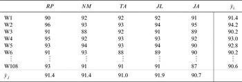
In this section, we introduce four measures of consistency of a group of m > 2 judges of n wines. Three of them are parametric, and one is nonparametric; two of them provide only a group measure of consistency, while the other two provide estimates of individual judge characteristics. To illustrate their use, we examine data from the website bordoverview.com, which contains ratings assigned by world-renowned critics from the United States and Europe for hundreds of Bordeaux wines from 2004 to 2012 vintages. In this study, we use the dataset from 2012, which contains 108 wines, each tasted by five wine critics: Robert Parker (RP, American), Neal Martin (NM, English), Tim Atkin (TA, English), Jeff Leve (JL, American), and Jane Anson (JA, English). The ratings consist of exact scores (e.g., 85) and range data, which we converted to their maximum bound (e.g., 95 for 93–95). The wines were rated by each critic and placed into one of 17 ordered categories ranging from 82 to 98, where a higher score means a better wine quality. Table 4 shows a subset of the data for the 5 judges of the 108 wines.
Example of Ratings on Bordeaux Wines

A. A Parametric Analysis: Intraclass Correlation (ICC)
The intraclass correlation can be used to assess the consistency of measurements made by multiple judges measuring the same quantity. ICC can be defined in different ways, depending on whether judges are considered random or fixed effects in an analysis of variance (ANOVA) model. The conceptual difference in these two models is defined by whether the judges are regarded as a random sample from a population of judges or whether the judges providing scores are themselves of interest. For the data in Table 4, we are interested in measuring consistency of these specific judges, so we consider the judges as fixed effects.
Let y ij be the score of wine i assigned by judge j. McGraw and Wong (Reference McGraw and Wong1996) proposed a two-way mixed effects model
 $$y_{ij} = \mu + \alpha _i + \beta _j + \epsilon _{ij}, \,\,\,i = 1, \cdots, n;\,\,j = 1, \cdots, m,$$
where μ denotes the population mean, α
i
is the wine random effect, assumed identically distributed with mean 0 and variance σ
α
2, β
j
is the judge fixed effect, and
 $ \epsilon _{ij} $
is the residual effect, also assumed identically distributed with mean 0 and variance σ
e
2. The ICC is then defined as
 $${\rho} _{ICC} = \displaystyle{{\sigma _\alpha ^2} \over {\sigma _\alpha ^2 + \sigma _e^2}}. $$
ICC ranges from 0 and 1 and can be interpreted as the proportion of total variance “between wines.” A larger value of ICC, or equivalently, a smaller value of σ e 2, indicates a higher level of judge agreement among judges.
An estimator of ρ ICC is
 $$\mathop {\hat \rho} \nolimits_{ICC} = \displaystyle{{MS_\alpha - MS_e} \over {MS_\alpha + (m - 1)MS_e}}, $$
where
 $MS_\alpha = \sum\nolimits_{i = 1}^n \,(\mathop {\bar y}\nolimits_{i +} - \mathop {\bar y}\nolimits_{ + +} )^2 /(n - 1)$
is the mean squared error for the wine factor.
 $\mathop {\bar y}\nolimits_{i +} $
denotes the mean score assigned by all the judges to the ith wine,
 $\mathop {\bar y}\nolimits_{ + j} $
denotes the mean score assigned by the jth judge on all the wines, and
 $\mathop {\bar y}\nolimits_{ + +} $
denotes the grand mean over all y
ij
s. The term
 $MS_e = \sum\nolimits_{i = 1}^n \,\sum\nolimits_{j = 1}^m \,(y_{ij} - \mathop {\bar y}\nolimits_{i +} - \mathop {\bar y}\nolimits_{ + j} + \mathop {\bar y}\nolimits_{ + +} )^2 /[(n - 1)(m - 1)]$
is the mean squared error for the residual effect. The estimate of ρ
ICC
for the Bordeaux data is
 $$\mathop {\hat \rho} \nolimits_{ICC} = \displaystyle{{25.249 - 4.211} \over {25.249 + (5 - 1)4.211}} = 0.500,$$
which shows a medium level of concordance among the five wine critics.
To obtain a confidence interval (γ L , γ U ) for ρ ICC , define ν 1 = (n − 1)(m − 1) and ν 2 = n − 1, and
 $$F_O = \displaystyle{{MS_\alpha} \over {MS_e}}, \,\,\,F_L = \displaystyle{{F_O} \over {F^ *}}, \,\,\,F_U = F_O F^ *, $$
where F * = F 1−α/2,ν 1, ν 2 is the upper 100(α/2)% tail of the F-distribution with ν 1 and ν 2 degrees of freedom (d.f.) (Shrout and Fleiss, Reference Shrout and Fleiss1979). Then
 $$ \gamma _{_L} = \displaystyle{{F_L - 1} \over {F_L + m - 1}},\,\,\, \gamma _{_U} = \displaystyle{{F_U - 1} \over {F_U + m - 1}}.$$
Based on these data, F O = 5.996, F L = 4.499, and F U = 8.213, and the 95% confidence interval for ρ ICC is (0.412, 0.591).
It should be noted the ICC in Equation (14) is defined as a ratio of variances, which must be nonnegative. Yet, when MS
α
is small relative to MS
e
in the ANOVA model,
 $\mathop {\hat \rho} \nolimits_{ICC} $
will be negative, with a lower bound of −1/ (m − 1). This generally will not occur, but when it does, it can be interpreted as indicating that ρ
ICC
is low or that Equation (13) does not fit the data well.
B. A Parametric Analysis: Product-Moment Correlations
Pearson's product-moment correlation (Equation (1)) can be used to measure judge agreement among m judges. Calculate the product-moment correlation r ij for each pair of judges J i and J j (i ≠ j;i, j = 1, …, m). The composite yields a correlation matrix
 $$R = \left( {\matrix{ 1 & {r_{12}} & \cdots & {r_{1m}} \cr {r_{21}} & 1 & \cdots & {r_{2m}} \cr \vdots & \vdots & \ddots & \vdots \cr {r_{m1}} & \cdots & \cdots & 1 \cr}} \right),\quad \quad {\rm where}\;r_{ij} = r_{\,ji}. $$
One overall measure of concordance is the average correlation among all pairs:
 $$g = \sum\limits_{i \ne j} \,r_{ij} /m(m - 1).$$
The value g = 1 is that of complete concordance, and a value of g = 0 is that of no correlation between the judges. However, the lower bound of g is constrained (because R is positive semidefinite) to g = − 1/(m − 1), which occurs when all pairs have r ij = − 1/(m − 1)r ij = − 1/(m − 1). The lower bound of g = −1 can occur only for m = 2 judges. Intuitively, the reason it is not possible for more discordance to occur among m > 2 judges is that if J 1 is perfectly negatively correlated with both J 2 and J 3, then J 2 and J 3 must be perfectly positively correlated.
Under the hypothesis of multivariate normality of the underlying scores and no concordance, g is approximately normally distributed with mean zero and variance Var(g) ≈ m(m − 1)/n. This allows inference of the hypothesis that the average ρ ij among the m judges is 0, based on the sample of wines rated. However, as noted previously, this is not usually an hypothesis of interest for expert wine judges. Rather, one is more likely to be interested in determining which judge is most consistent with the other judges in terms of the values given to each wine. To do this, define the column means from the correlation matrix,
 $$r_i = \sum\limits_{i \ne j} \,r_{ij} /(m - 1),$$
for i = 1, …, m. Now order the column means
 $$r_{[1]} \ge r_{[2]} \ge \ldots \ge r_{[m]}. $$
This ranking provides a measure of consistency in the sense that J [1] is in more agreement with the other m − 1 judges than J [2]; J [2] is in more agreement with the others than J [3], and so on. The gap r [i] − r [i−1] provides a measure of the degree to which J [i] dominates J [i−1].
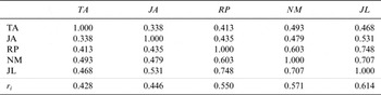
For the Bordeaux data, the matrix R and the column means r i are presented in Table 5, where the columns of R representing judges are ordered by their consistency. The average between judge correlation is g = 0.522. Jeff Leve (r 4 = 0.614) shows the most agreement with the other judges, and Tim Atkin (r 3 = 0.428) shows the least. This information is based on pairwise comparisons, which provides more information than a single measure of concordance, such as the ICC. In the next section, we describe a method that provides still more information about the individual differences in the judge's score characteristics.
Pairwise Pearson's Correlation

C. A Parametric Analysis: Bayesian Ordinal Model
Cao and Stokes (Reference Cao and Stokes2010) proposed a Bayesian ordinal model to evaluate wine judge performance by identifying which of the three judge characteristics—bias, discrimination ability, and random variation—are responsible for disagreement among judges. Judge bias measures the systematic difference between a judge's score and the average score of all judges. Based on the bias, one can identify whether a judge is relatively generous, neutral, or stringent in his or her assignment of scores. Judge discrimination measures a judge's ability to distinguish wines based on their quality. Judges with a higher degree of discriminating power can distinguish wines more easily. Judge variation measures the amount of judgment error in a judge's assessment of wine quality.
Suppose judges assign scores by first estimating the wine quality on a continuously valued scale and then comparing it with category cutoffs, which are the same for all judges. Let θ i (i = 1, …, n) denote the underlying unobserved quality of wine i, x ij the estimate of θ i by judge j, and y ij the observed ordinal score assigned by judge j on wine i. Then the continuous estimate of the ith wine's quality θ i by judge j is modeled as
 $$x_{ij} = \alpha _j + \beta _j \theta _i + e_{ij}. $$
The quantity e ij is the judgment error made by judge j on his assessment of wine i, and is assumed to have a normal distribution with mean zero and a judge-specific variance σ j 2 for all wines. The parameter α j quantifies the bias for judge j, and β j measures the discrimination ability of judge j. Then y ij takes the ordinal score of s if x ij falls between category cutoffs c s−1 and c s , that is
 $$y_{ij} = s \quad {\rm if}\,{\rm and}\,{\rm only} \,{\rm if}\;\,c_{s - 1} < x_{ij} \le c_s. $$
The quantities c s denote the upper cutoff of ordinal level s for all judges. For more details on the prior assignment of the parameters and Bayesian computation, see Cao and Stokes (Reference Cao and Stokes2010).
A judge's performance can be evaluated based on the correlation between his/her assigned ratings and the estimates of wine latent quality θ
i
's, and the correlation is denoted by r
B
. Table 6 shows the results of the Bayesian ordinal model. Jeff Leve's ratings have the highest agreement (i.e., value of r
B
) with the estimates of latent quality of the wines (i.e.,
 $\mathop {\hat \theta} \nolimits_i $
's), which is attributed to his larger discrimination level and smaller measurement error. The ratings assigned by Tim Atkin have the least agreement with the
 $\mathop {\hat \theta} \nolimits_i $
's due to his smaller discrimination level and larger measurement error.
Analysis Based on the Bayesian Ordinal Model

Tables 5 and 6 agree on the most and least consistent of the judges but reverse the order of the middle pair (i.e., NM and RP). Compared to the previous measures (i.e.,
 $\mathop {\hat \rho} \nolimits_{ICC} $
and g), which provide an aggregate assessment of judge agreement, the Bayesian model provides insight into what makes judges differ.
D. A Nonparametric Analysis: Kendall's Coefficient of Concordance
We now return to global measures of consistency for multiple judges but without the assumption of normality that the parametric measures require. Kendall's coefficient of concordance W is such a measure (Kendall and Smith, Reference Kendall and Smith1939). Let R
ij
denote the rank of wine i (i = 1, L, n) based on the ratings assigned by judge j (j = 1, L, m), and
 $R_{i +} = \sum\nolimits_{j = 1}^m \,R_{ij} \,(j \ne i)$
denote the total rank given to wine i by the m judges. The mean of the total of the ranks is
 $\bar R = m(n + 1)/2$
and denote the sum of squared deviations of each total rank from the overall mean by
 $S = \sum\nolimits_{i = 1}^n \,(R_{i +} - \bar R)^2 $
. Kendall's W is defined as
 $$W = \displaystyle{{12S} \over {m^2 n(n^2 - 1)}},$$
where W is the ratio of the variance of the row sums of ranks R i+ divided by the maximum value of the variance under complete judge agreement. Kendall's W ranges from 0 to 1, where W = 1 indicates that all judges have ranked the wines in the same order. When the ratings from the m judges are independent (no concordance), W is not exactly 0. In this case, W has an expectation of E(W) = 1/m with variance Var(W) = 2(m − 1)/m 3(n − 1) (Kendall, Reference Kendall1962). For example, independent rankings from three judges will yield W = 0.33 on average. The statistic W approaches zero as m increases (by the order of 1/m 2) and also as n increases. Doubling the number of judges decreases the variance by 1/4.
A simple function of W makes it interpretable as a nonparametric equivalent of g in Equation (17). Specifically, the average of Spearman's rank correlations,
 $\bar r_s $
, over the m(m − 1)/2 pairs of judges can be computed as,
 $$\bar r_s = \displaystyle{{mW - 1} \over {m - 1}}.$$
In the case of perfect judge agreement,
 $\bar r_s = 1$
and W = 1. When W = 0,
 $\bar r_s = - 1/(m - 1)$
, which means there is actually disagreement among judges.
Siegel (Reference Siegel1956) proposed an adjusted Kendall's W when ties are present. Define
 $$T_j = \sum\limits_{i = 1}^{g_j} \,(t_i^3 - t_i ),$$
where t i is the number of tied ranks in the group of ranks for wine i, and g j is the number of groups of ties of the ranks given by judge j. Then Kendall's W corrected for ties is
 $$W = \displaystyle{{12S} \over {m^2 n(n^2 - 1) - m\sum\nolimits_1^m \,T_j}}. $$
Tables of critical values exist for small values of m and n (Siegel, Reference Siegel1956). For larger samples, an approximate test of significance is obtained from the statistic m(n − 1)W, which has a chi-square distribution with n − 1 degrees of freedom under the assumption of no association (Friedman, Reference Friedman1937). For the Bordeaux data, we have
 $$W = \displaystyle{{12 \times 1585745} \over {5^2 \times 108 \times (108^2 - 1) - 5 \times 81432}} = 0.612$$
with a p-value of 3.34E–24, indicating there is a significant amount of agreement among the judges.
IV. Meta-Analysis for m Judges and n Wines
The term meta-analysis has been used in methods for combining the results of independent studies (Cooper et al., Reference Cooper, Hedges and Valentine2009). In the medical context, it relates to how to combine the results of independent studies, each one designed to evaluate a treatment effect.
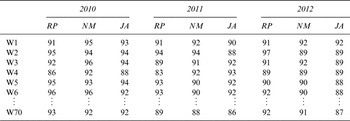
In the previous sections, we have studied different measures of judge agreement with two or more judges. In this section, we focus on testing whether the judge agreement patterns are homogeneous across different datasets. This falls in the category of meta-analysis. The data model in this section relates to the case in which there are wine tastings across k years (or at k sites). That is, there are the same m judges and n wines at each year. The Bordeaux data contain three judges' tasting scores (RP, NM, and JA) across three years (2010, 2011, and 2012) on the same set of 70 different wines (i.e., k = 3, m = 3, and n = 70). Table 7 shows a subset of the data.
Example of Ratings on Bordeaux Wines over Three Years

A. A Parametric Analysis: Concordance Across Years Based on Correlations
From the Bordeaux wine data in Table 7 we generate three matrices of Pearson correlations
 $$\hskip10pt R_{2010} = \left( {\matrix{ 1 & {0.606} & {0.692} \cr {0.606} & 1 & {0.587} \cr {0.692} & {0.587} & 1 \cr}} \right),\quad R_{2011} = \left( {\matrix{ 1 & {0.580} & {0.492} \cr {0.580} & 1 & {0.447} \cr {0.492} & {0.447} & 1 \cr}} \right), \quad R_{2012} = \left( {\matrix{ 1 & {0.585} & {0.566} \cr {0.585} & 1 & {0.509} \cr {0.566} & {0.509} & 1 \cr}} \right),$$
from 2010, 2011, and 2012. Each matrix shows the correlation of the scores among the three judges, where the rows and columns correspond to RP, NM, and JA, in that order. To investigate whether the years differ with respect to concordance, we test the homogeneity of correlation matrices.
There are several alternative tests for the homogeneity of correlation matrices, all based on the assumption that the correlation matrices arise from a multivariate normal model. The likelihood ratio test is rather complicated, and, instead, we adopt a simpler test proposed by Larntz and Perlman (Reference Larntz, Perlman, Berger and Gupta1988) that still provides a correct significance level. Apply the Fisher transformation (Equation (2)) to each correlation coefficient r
ij
(h) (i, j = 1, …, m) in the hth (h = 1, …, k) sample correlation matrix R
h
, obtaining z
ij
(h). Define the element-wise means
 $\bar z_{ij} = \sum\nolimits_{h = 1}^k \,z_{ij}^{(h)} /k$
and variances
 $\nu _{ij} = (n - 3)\sum\nolimits_{h = 1}^k \,(z_{ij}^{(h)} - \bar z_{ij} )^2 $
, where n is the number of wines. Then the test statistic is
 $$T = max \{ \nu _{ij}, \,1 \le i < j \le m \}. $$
The null hypothesis that the sample correlation matrices R
1, …, R
k
come from a population with a common correlation matrix is rejected if
 $T > \chi _{k - 1}^2 (\tilde \alpha )$
, where
 $ \chi _{k - 1}^2 (\tilde \alpha )$
is the
 $\tilde \alpha $
th percentile of the χ
k−1
2 distribution. To achieve a given significance level α, we compute
 $\tilde \alpha = (1 - \alpha )^{2/m(m - 1)} $
from α and use
 $\tilde \alpha $
in the chi-square test. Because the test statistic (Equation (23)) is based on the maximum of ν
ij
(
 $1 \le i < j \le m$
), the test is generally conservative. For large m, the data has to show a strong difference to reject the null hypothesis.
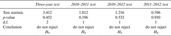
Table 8 provides a summary of the three-year and two-year comparisons. Based on the chi-square test, there is a lack of evidence to conclude that the agreement among the three judges is heterogeneous across the three years (p = 0.452). This conclusion confirms the noticeable similarity among the three correlation matrices. The subsequent pairwise comparisons yield similar test results (i.e., do not reject H 0), which is consistent with the conclusion on the across-the-three-year comparison. The direct comparison of correlation matrices R 2010, R 2011, and R 2012 provides more details on the judge agreement patterns. Both the order and the magnitude of the pairwise correlations remain similar between 2011 and 2012, i.e., r 12>r 13>r 23, g 2011 = 0.51, g 2012 = 0.55, where g is the average correlation among all pairs in Equation (17). In contrast, the order of the pairwise correlations in 2010 has changed to r 13>r 12>r 23, and the average level of judge agreement is g 2010 = 0.63. The fact that g 2010 is the largest and g 2011 is the smallest among the three gs and the order of the pairwise correlations differs between the two years suggests that the judge agreement between 2010 and 2011 is the weakest. This conclusion is confirmed by a smaller p-value between the 2010 and 2011 comparison (p = 0.196) compared to the other two-year comparisons (p-values are 0.532 and 0.910, respectively).
Test for the Homogeneity of Correlation Matrices

B. A Nonparametric Analysis: Concordance Across Years
In order to avoid a test based on the assumption of an underlying normal distribution, we can use a nonparametric procedure to assess judge consistency across years or sites. Specifically, we use Kendall's coefficient of concordance as a basis of comparison, rather than the product- moment correlation coefficient. Again we illustrate the method with the Bordeaux data from Table 7. As in the previous section, we test the hypothesis that judge agreement is consistent over time against the hypothesis that it is not. If the relationship among the judges' ratings were consistent, an exchange of a year's set of scores for another year's for each of the wines would not change the distribution of Kendall's W nor would it change the relationship among the coefficients from year to year. Based on this rationale, we propose a permutation test using Kendall's W (Equation (22)). For the Bordeaux data in Table 7, we permute the year indices for each wine i to produce a null dataset under the hypothesis that judge agreements are comparable over time. Note that each year produces a value of W. A test statistic that measures the discrepancy in consistency can be calculated from each permuted dataset and an empirical null distribution produced. The test statistic we propose is
 $$RW = \displaystyle{{W_{min}} \over {W_{max}}}, $$
where W min and W max are the minimum and the maximum of the Ws respectively. The p-value for this comparison is the tail probability of RW based on the observed data for the empirical null distribution. This permutation test can be extended to multiple years, where the year index are permutated for each wine.
Applying this method to test whether the levels of judge agreement are similar across the three years for the Bordeaux wine data yielded the following results. The p-values, based on 20,000 permutations, are 0.525 for the three-year comparison, 0.260 for the 2010–2011 comparison, 0.535 for the 2010–2012 comparison, and 0.716 for the 2011–2012 comparison, respectively. Taken together, we can reach the same conclusion as the one in the parametric analysis—that is, levels of judge agreement are similar across the three years, where the similarity of judge agreement between 2010 and 2011 is relatively weaker.
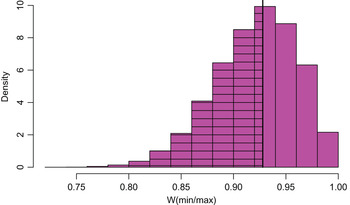
To add more detail to the permutation test, we include Figure 1, which is the histogram of RW's empirical null distribution for the three-year comparison. The vertical line shows the observed RW, which is RW = 0.675/0.727 = 0.928. The p-value is the proportion of RW under the empirical null distribution that is less than the observed RW, which is the marked area below the vertical line in the histogram. As mentioned above, the p-value is 0.525 for the three-year comparison.
The Empirical Null Distribution of R W for the Three-Year Comparison

V. Other Novel Analyses on Wine Tasting
Tasting events provide a rich source of alternative scenarios and analyses. They raise many issues in addition to judge agreement or consistency. We here introduce several different models for future consideration.
A. Which Wine is Better? Analysis for Two Wines and m Judges
In this tasting model, two wines (A and B) are to be compared by m judges. The central goal is to determine which wine is superior. Suppose the data are obtained from a blinded tasting of two wines from m judges. Each judge gives a score of 1 if wine A is preferable to wine B, and a 2 if wine B is preferable to A. Ties are denoted by 0 and are omitted from the analysis. Table 9 provides an illustrative example of such data for two wines and 10 judges.
Scores for 2 Wines and 10 Judges

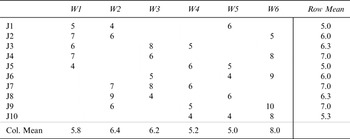
BIB Design for the Configuration: n = 6, m = 10, j = 3, w = 5, λ = 2

The ANOVA Analysis

Define n 1 as the number of ones (i.e., number of judges who prefer wine A) and n 2 as the number of twos (i.e., number of judges who prefer wine B). Then a test statistic for deciding whether the differences in the preference between the two wines are due to chance is
 $$C = \displaystyle{{(\vert n_1 - n_2 \vert - 1)^2} \over {n_1 + n_2}}. $$
Under the null hypothesis of no preference, the statistic C has an approximate chi-square distribution with 1 d.f. If the test result is significant, then it indicates that one wine is significantly preferable to the other. Otherwise, the preference is not statistically significant.
This test, called the sign test, was introduced by Dixon and Mood (Reference Dixon and Mood1946). For small samples, exact significance levels are provided by Dixon and Massey (Reference Dixon and Massey1969). Define p = n 1/(n 1 + n 2) as the proportion of ones. then |n1 − n 2|/(n 1 + n 2) = 2|p − 0.5|. So the statistic C measures the departure from equality of zeros and ones. The −1 in C is a continuity correction to make the distribution closer to the chi-square distribution.
For the data in Table 9, n 1 = 6, n 2 = 2, and C=(|6 − 2| − 1)2/8 = 1.125, which has a p-value of 0.29 obtained from the chi-square distribution table. This indicates that no difference in preference between the two wines was detected. In general, a larger sample size of judges is required to detect significance. For a 5% level of significance, the chi-square critical value is 3.81. Thus, for n 1 = 12, n 2 = 4 the value of C is 3.06, which is not significant. However, for n 1 = 18, n 2 = 6 (a threefold increase) the value of C is 5.04, which is highly significant.
This sign test is to determine which of two wines is better. Quandt (Reference Quandt2007) considered the case in which there are two types of wines being tasted and each type may contain a number of wines. Quandt proposed a permutation test based on the rank sums to determine whether the wines of one type on the whole are more favored than the wines of the other type.
B. Paired Comparison: Network
Paired comparisons is an efficient method for ranking n items. It involves comparing items two at a time. This is a recognized method that optometrists use to find the single best prescription for eyeglasses. However, there is a price in that the method requires n(n − 1)/2 comparisons instead of n. For example, a comparison of 10 wines requires 45 comparisons instead of 10. This design has the advantage in terms of achieving a more accurate evaluation in that most people are capable of ranking only a small number of items (i.e., five to nine) at a time (Miller, Reference Miller1956).
Pairwise comparisons also provide a method for the analysis of consistency. Denote the preference “A is preferred to B” by A→B. For three wines, A, B, and C, if A is preferred to B, B is preferred to C, and C is preferred to A, then there is a loop and an inconsistency. For a moderate number of wines with similar scores, such inconsistencies are to be expected. To further clarify this point, there are eight possible preference configurations among three wines:
 $$\eqalign{& \left( 1 \right)A \to B \to C \to A,\left( 2 \right)A \to B \to C,\left( 3 \right)B \to C \to A,\left( 4 \right)C \to A \to B, \cr & \left( 5 \right)A \to C \to B \to A, \left( 6 \right)A \to C \to B,(7)C \to B \to A,(8)B \to A \to C.} $$
Of these, only (1) and (5) are inconsistent, so with a random configuration, we expect a 25% chance of inconsistency among the preference configurations.
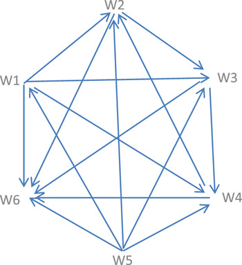
We present a network approach to study judge agreement based on pairwise comparisons of wines. In the network graph, the wines to be ranked are the vertices, and the judges' preferences are the edge flows connecting the vertices. Figure 2 provides an example of the network involving six wines. When judges all agree with one another, there will be no inconsistent triples in the network. The more inconsistent triples there are, the more serious is the lack of agreement among judges. So we can use the proportion of inconsistent triples among all triples as the test statistic (denoted as p inc ) to measure judge agreement.
The Network of Pairwise Comparisons for Six Wines

We use the example in Figure 2 to demonstrate the idea. The network also can be presented by an n × n matrix
 $$V = \left[ {\matrix{ 0 & 0 & 1 & 0 & 0 & 1 \cr 1 & 0 & 1 & 0 & 0 & 1 \cr 0 & 0 & 0 & 0 & 0 & 1 \cr 1 & 1 & 1 & 0 & 1 & 1 \cr 1 & 1 & 1 & 0 & 0 & 1 \cr 0 & 0 & 0 & 0 & 0 & 0 \cr}} \right],$$
in which the element v ij = 1(i ≠ j; i, j = 1, …, n; n = 6)) indicates that vertex i is preferred to vertex j. The diagonal element v ii = 0 and v ji = 1 − v ij (i ≠ j) is the symmetric comparison. There are several ways to define v ij : by direct pairwise comparison, by comparing the score average between each pair of wines, or by the majority of votes between each pair, and so on. From Figure 2, the triples that consist of wines W2, W3, and W4 are inconsistent. Specifically, we have W2→W3→W4→W2.
The pairwise ranking matrix when there is no agreement between judges (denoted as V random ) can be constructed by randomly assigning a 0 and 1 to each v ij (i < j), the upper diagonal elements in V random , and setting v ji = 1 − v ij . The empirical null distribution of the proportion p inc of inconsistencies is then obtained as the percentage of inconsistencies over all random choices of preferences. The p-value is the proportion of p inc under the empirical null distribution that is less than the observed p inc . In the context of this example, the p-value is 0.047, which indicates that the judge agreement based on the triple-wise comparison is significant.
C. The Design of a Wine-Tasting Event
As the number of wines to be tasted increases, it becomes more difficult to score or rank the wines. For example, about 2,500 different wines competed in the California State Fair Wine Competition in 2009. Altogether 68 judges were assigned to 17 panels, with 4 judges in each panel, and each panel evaluated about 150 wines over two days. The wines were organized into flights, which are collections of wines of a similar type. Each panel of judges evaluated a number of flights per day, ranging from three flights of large size (with more than 30 wines) to 10 flights of small size (with less than 10 wines). With the intensive tasting task, judges become exhausted, and the wine-tasting results can become less reliable. This raises the question of whether an analysis can be generated with fewer tastings, which in turn implies that there will be less difficulty in judging the wines.
When each judge tastes each wine, the design is called a completely balanced block design. By comparison, a balanced incomplete block design (BIB) permits an analysis that yields similar comparisons but saves observations. The development of BIB originated in an agricultural context in the 1930s by R.A. Fisher and F. Yates (Reference Fisher and Yates1974) and is well documented in books on the design of experiments. See, for example, Amerine and Roessler (Reference Amerine and Roessler1976), who proposed using a BIB for wine-tasting events. We now describe the method.
Because we desire a balance in the design, not all combinations of the number of judges and the number of wines permit a BIB. To fix ideas and to clarify the ingredients in the design, we focus on Table 10, in which n = 6 wines are scored by m = 10 judges, in which each judge tastes j = 3 wines, and each wine is scored by w = 5 judges. Furthermore, each wine is compared twice (λ = 2) with every other wine. Not all choices of n, m, j, w, λ can be constructed to yield a BIB design. There are two restrictions:
 $$Mj = nw$$
 $$ \lambda (n - 1) = w(\,j - 1).$$
The book Statistical Tables for Biological, Agricultural and Medical Research (Fisher and Yates, Reference Fisher and Yates1974, p. 56) and Cochran and Cox (Reference Cochran and Cox1957) provide examples of BIB designs for different values of n, m, j, w, and λ. For example, the configuration n = 6, m = 10, j = 3, w = 5, λ = 2 satisfies the restrictions, so this BIB design has a total of 30 tastings instead of 60 under a completely balanced block design.
Table 10 presents an example of the above configuration, in which the scoring is on a 10-point scale with 1 being the lowest and 10 being the highest score. Here, we see that wines W1 and W2 are tasted by judges J1 and J2, that wines W1 and W5 are tasted by judges J1 and J5, and so on. Furthermore, wines W4 and W6 are compared twice, once by judge J9 and once by judge J10.
The data is analyzed using ANOVA under the BIB design. Let y il be the score given by the lth judge to the ith wine, where i = 1, L, n, and l = 1, L, m. Further, suppose each score has a wine effect and a judge effect, so that
 $$y_{il} = \mu + \alpha _i + \beta _l + \epsilon _{il}, $$
where μ is the overall mean, α
i
is the mean effect of the ith wine, β
l
is the mean effect of the lth judge, and
 $ \epsilon _{il} $
is the random effect. Note that the degrees of freedom for the judges is m − 1, and for the wines is n − 1. The degrees of freedom for the total is N − 1, where N = nw = mj. Table 11 shows the ANOVA table of results in which MSE = SSE/d.f. The test of judge effect (β
1 … β
10) is obtained from Table 11 as MSE(judges)/MSE(error) = 1.86/2.46 = 0.75 and yields a p-value from the F-test as 0.66. With a significance level of 0.05, we reject the null hypothesis that the mean effects of judges are the same.
It should be noted that the test based on this ANOVA model is not for judge agreement in terms of concordance of wine ratings. It is to test whether judges have similar average ratings. Judges who have similar average ratings may have poor consensus. For example, if one judge assigns score 4, 5, 6 to three wines, and another judge assigns score 6, 5, 4 to the same three wines, then the average ratings between the two judges are the same, yet the orders of the ratings are completely opposite.
VI. Discussion
In this paper, we have provided a tutorial on data analysis of wine tasting events. Specifically, we focused on evaluating judge agreement in the cases of two judges, m judges, and comparison across years in Sections II to IV. In Section V, we provided other analyses on comparing two wines, pairwise comparison of wines based on a network and balanced incomplete block design to reduce the tasting load for judges. We plan to further develop some of the three topics in the future. In particular, one topic is how to use the network to produce an aggregate ranking of the wines and a valid measure on the significance of the ranking. A second area of research is to compare the effects of using a balanced incomplete block design with a completely balanced block design.
All the analyses in the paper are conducted in R, free statistical software. The R code is provided in the online supplementary file.
Supplementary Material
For supplementary material accompanying this paper visit http://dx.doi.org/10.1017/S1931436114000261.