1. Introduction
Various experimental and simulation studies of flowing blood have shown that red blood cells (RBCs) are concentrated in the centre of the blood vessel. This can be explained by a non-inertial lift force, arising from cell–wall and cell–cell hydrodynamic interactions, the high deformability of RBCs and their non-spherical shapes, see e.g. Kumar & Graham (Reference Kumar and Graham2012) for a recent review. The non-inertial lift force results in a migration of RBCs towards the centre of the vessel and an RBC-free layer near the wall. Differences in size, shape and deformability are assumed to lead to different non-inertial lift forces, which results in a separation of cells with different mechanical properties within the blood vessel. White blood cells (WBCs) have a near-spherical shape and are not very deformable and are therefore mechanically different from RBCs. The non-inertial lift force of WBCs is expected to be much lower than that on RBCs, or even zero in the limit of a rigid-body approximation for WBCs (Goldsmith & Mason Reference Goldsmith and Mason1961; Bretherton Reference Bretherton1962). This suggests that WBCs may get marginated to the RBC-free layer near the wall. This effect requires the interaction of RBCs and WBCs and is of utmost importance for a well-functioning immune system, which requires the adhesion of WBCs to the vessel wall.
For low Reynolds numbers the phenomenon is in principle understood. However, in this regime detailed investigations also show a non-trivial dependence of WBC margination on various blood flow properties, such as haematocrit
 $H_{t}$
, vessel geometry and RBC aggregation (Pearson & Lipowsky Reference Pearson and Lipowsky2000; Abbitt & Nash Reference Abbitt and Nash2003; Jain & Munn Reference Jain and Munn2009). One example is a pronounced margination within an intermediate range of
 $H_{t}\approx 0.2{-}0.3$
, and reduced WBC margination for lower and higher
 $H_{t}$
. Only recently could such behaviour be explained through simulation studies in two dimensions (Fedosov, Fornleitner & Gompper Reference Fedosov, Fornleitner and Gompper2012). It is argued that for low
 $H_{t}$
, WBC margination turns out to be weak due to a low concentration of RBCs and thus less interaction, while at high
 $H_{t}$
WBC margination is attenuated due to interactions of marginated WBCs with RBCs near a wall, which significantly limit the time WBCs spend near a wall. This argumentation is confirmed by 3D simulations in an idealized blood vessel (Fedosov & Gompper Reference Fedosov and Gompper2014; Takeishi et al.
Reference Takeishi, Imai, Nakaaki, Yamaguchi and Ishikawa2014).
The situation changes, if inertial effects come into play. Now, an inertial lift force is present, which acts on all cells at intermediate-Reynolds-number flows (Geislinger & Franke Reference Geislinger and Franke2014). As a consequence WBCs also experience a lift force, even in the limit of a rigid-body approximation. This contradicts the simple explanation for WBC margination given above and indeed leads to decreasing margination for an increasing Reynolds number. We vary the Reynolds number, considering values of order
 $10^{-4}$
,
 $10^{-2}$
, 1 and 10, corresponding to different regions in the cardiovascular system (Formaggiam, Quarteroni & Veneziani Reference Formaggiam, Quarteroni and Veneziani2000). Reynolds numbers of order unity or higher have been reported in large blood vessels, such as arterioles and arteries (Prothero & Burton Reference Prothero and Burton1962; Ku Reference Ku1997), especially if the vessels are constricted due to diseases such as thrombosis (see e.g. Vennemann, Lindken & Westerweel Reference Vennemann, Lindken and Westerweel2007; Bark & Ku Reference Bark and Ku2010).
The paper is organized as follows. In § 2 we first review existing modelling approaches. Next our approach is described in detail. It is based on a Helfrich-type curvature-elastic model (Helfrich Reference Helfrich1973). We consider various constraints concerning membrane inextensibility and area conservation for the RBCs and treat WBCs using a rigid-body approximation or as objects with a weakly extensible membrane. We further consider cell–cell interactions and model the fluid flow of the blood plasma and the internal fluids using the incompressible Navier–Stokes equations. We prove thermodynamic consistency of the model and briefly discuss the numerical approach. This approach requires only measurable parameters as input and thus in principle allows for quantitative predictions. However, we will restrict our simulations to two dimensions. The effect of various parameters on the margination of WBCs is discussed in § 3, first reproducing known results for low-Reynolds-number regimes and then analysing the effect of intermediate Reynolds numbers. The decreasing effect of the Reynolds number on WBC margination is discussed in detail and explained by investigations of the inertial lift force on a single RBC and a single WBC. Finally, we draw conclusions in § 4.
2. Methods and models
2.1. Previous models
Previous simulation studies, which have been performed to describe WBC margination, are based on strong model assumptions. The simulation approach (Freund Reference Freund2007) assumes an incompressible Stokes flow, the cells are modelled with a linear elastic membrane and a global area constraint is enforced. A boundary integral formulation is used for numerical discretization. More recently, a particle-based Lagrangian approach was used (Fedosov et al. Reference Fedosov, Fornleitner and Gompper2012; Fedosov & Gompper Reference Fedosov and Gompper2014). Here, RBCs and WBCs are described by a network model, where the cells are represented through triangulated surfaces. Penalty terms are used to ensure global volume and global area conservation as well as local area conservation for each surface element. The approach therefore guarantees inextensibility for sufficiently small surface elements. Each membrane point is connected to the fluid through viscous friction. The dynamics of the fluid flow is described by the smoothed dissipative particle dynamics (SDPD) method, an approximation for the Navier–Stokes equations which is only precise, if the particle density is large enough. Furthermore, the incompressibility of the fluid is not guaranteed a priori and has to be controlled. In Takeishi et al. (Reference Takeishi, Imai, Nakaaki, Yamaguchi and Ishikawa2014), a finite element approach is used for the RBCs, which are modelled as biconcave capsules and a Lattice–Boltzmann method for the fluid flow. The problems are coupled through an immersed boundary method.
Our approach is fully continuous and considers RBCs using a Helfrich-type curvature elastic model with an inextensibility constraint. WBCs are modelled either as rigid bodies or again with a Helfrich-type curvature elastic model, but with a constraint allowing for weak extensibility. Furthermore, we will consider the full Navier–Stokes equations to account for inertia effects in the plasma. According to previous studies (N’Dri, Shyy & Tran-Son-Tay Reference N’Dri, Shyy and Tran-Son-Tay2003) we also consider the internal fluid of the RBCs and WBCs as an incompressible Newtonian fluid, neglecting internal structures and the nucleus in WBCs.
2.2. Helfrich-type models
Helfrich-type modelling approaches have been applied to understand the complex motions and shape changes RBCs undergo within a flow field, e.g. tank-treating (TT) and tumbling (TB) motion (Fischer, Stöhr-Liesen & Schmid-Schönbein Reference Fischer, Stöhr-Liesen and Schmid-Schönbein1978). Within a low-Reynolds-number regime, the Stokes limit is valid and various numerical approaches have also been considered in this limit to analyse the TT and TB motion (Kraus et al. Reference Kraus, Wintz, Seifert and Lipowsky1996; Biben & Misbah Reference Biben and Misbah2003; Beaucourt et al. Reference Beaucourt, Rioual, Seon, Biben and Misbah2004; Biben, Kassner & Misbah Reference Biben, Kassner and Misbah2005; Veerapaneni et al. Reference Veerapaneni, Gueyffier, Zorin and Biros2009; Ghigliotti, Biben & Misbah Reference Ghigliotti, Biben and Misbah2010; Kim & Lai Reference Kim and Lai2010; Sohn et al. Reference Sohn, Tseng, Li, Voigt and Lowengrub2010; Zhao & Shaqfeh Reference Zhao and Shaqfeh2011). All models consider a membrane-free energy
 $$\begin{eqnarray}\displaystyle \mathscr{E}=\int _{{\it\Gamma}}\frac{1}{2}b_{N}(H-H_{0})^{2}\,\text{d}{\it\Gamma}, & & \displaystyle\end{eqnarray}$$
with membrane
 ${\it\Gamma}(t)$
, mean curvature
 $H$
, spontaneous curvature
 $H_{0}$
and normal bending rigidity
 $b_{N}$
. Lagrange multipliers are used to enforce a global area constraint or the stronger inextensibility constraint. The jump condition for the fluid stress tensor
 $\unicode[STIX]{x1D64E}=\unicode[STIX]{x1D61A}_{0,i}=-p\unicode[STIX]{x1D644}+{\it\nu}_{0,i}\unicode[STIX]{x1D63F}$
, with pressure
 $p$
, fluid viscosity
 ${\it\nu}_{0}$
, cell viscosity
 ${\it\nu}_{i}$
and deformation tensor
 $\unicode[STIX]{x1D63F}=\boldsymbol{{\rm\nabla}}\boldsymbol{v}+(\boldsymbol{{\rm\nabla}}\boldsymbol{v})^{\text{T}}$
, with velocity
 $\boldsymbol{v}$
, along the membrane then reads
 $$\begin{eqnarray}\displaystyle & \displaystyle [\unicode[STIX]{x1D64E}\boldsymbol{\cdot }\boldsymbol{n}]_{{\it\Gamma}}=\frac{{\it\delta}\mathscr{E}}{{\it\delta}{\it\Gamma}}+{\it\lambda}_{\mathit{global}}\,H\boldsymbol{n}\quad \text{global area constraint,} & \displaystyle\end{eqnarray}$$
 $$\begin{eqnarray}\displaystyle & \displaystyle [\unicode[STIX]{x1D64E}\boldsymbol{\cdot }\boldsymbol{n}]_{{\it\Gamma}}=\frac{{\it\delta}\mathscr{E}}{{\it\delta}{\it\Gamma}}+{\it\lambda}_{\mathit{local}}\,H\boldsymbol{n}+\boldsymbol{{\rm\nabla}}_{\!{\it\Gamma}}{\it\lambda}_{\mathit{local}}\quad \text{local inextensibility constraint}, & \displaystyle\end{eqnarray}$$
with outer normal
 $\boldsymbol{n}$
and the surface gradient
 $\boldsymbol{{\rm\nabla}}_{\!{\it\Gamma}}=\unicode[STIX]{x1D64B}\boldsymbol{{\rm\nabla}}$
, where
 $\unicode[STIX]{x1D64B}=\unicode[STIX]{x1D644}-\boldsymbol{n}\otimes \boldsymbol{n}$
denotes the projection operator. Index 0 thereby denotes the fluid phase and index
 $i$
the cell phase. The Lagrange multipliers
 ${\it\lambda}_{\mathit{global}}$
and
 ${\it\lambda}_{\mathit{local}}$
are functionals of the fluid velocity
 $\boldsymbol{v}$
and are obtained by requiring
 $\text{d}/\text{d}t\int _{{\it\Gamma}}\,\text{d}{\it\Gamma}=\int _{{\it\Gamma}}H\boldsymbol{v}\boldsymbol{\cdot }\boldsymbol{n}\,\text{d}{\it\Gamma}=0$
for the global area constraint and
 $\boldsymbol{{\rm\nabla}}_{\!{\it\Gamma}}\boldsymbol{\cdot }\boldsymbol{v}=0$
along
 ${\it\Gamma}(t)$
for the local inextensibility constraint. The jump condition for the velocity reads
 $[\boldsymbol{v}]_{{\it\Gamma}}=0$
.
The linearity of the Stokes problem allows for efficient decoupled algorithms to solve for the Lagrange multipliers (Biben & Misbah Reference Biben and Misbah2003; Sohn et al. Reference Sohn, Tseng, Li, Voigt and Lowengrub2010; Zhao & Shaqfeh Reference Zhao and Shaqfeh2011). However, in regimes with the Reynolds number being of order unity or higher, the Stokes limit is at least questionable. Modelling approaches, which consider inertia effects, have been introduced recently (Laadhari, Saramito & Misbah Reference Laadhari, Saramito and Misbah2012; Salac & Miksis Reference Salac and Miksis2012; Aland et al. Reference Aland, Egerer, Lowengrub and Voigt2014). All have found that the classical TB behaviour is no longer observed at moderate Reynolds numbers. As such, a suppression of TB motion could have far reaching consequences also for the interaction of RBCs and thus also the margination of WBCs. In the following, we will consider the full Navier–Stokes equations, which read inside and outside the RBCs
 $$\begin{eqnarray}\displaystyle & {\it\rho}(\partial _{t}\boldsymbol{v}+\boldsymbol{v}\boldsymbol{\cdot }\boldsymbol{{\rm\nabla}}\boldsymbol{v})-\boldsymbol{{\rm\nabla}}\boldsymbol{\cdot }\unicode[STIX]{x1D64E}=0, & \displaystyle\end{eqnarray}$$
 $$\begin{eqnarray}\displaystyle & \boldsymbol{{\rm\nabla}}\boldsymbol{\cdot }\boldsymbol{v}=0, & \displaystyle\end{eqnarray}$$
with density
 ${\it\rho}={\it\rho}_{0,i}$
. The global area constraint can be treated explicitly, which was e.g. used by Bonito, Nochetto & Pauletti (Reference Bonito, Nochetto and Pauletti2011) within a front tracking method, proposed by Du, Li & Liu (Reference Du, Li and Liu2007) and used by Haußer et al. (Reference Haußer, Li, Lowengrub, Marth, Rätz and Voigt2013) and Marth & Voigt (Reference Marth and Voigt2014) for a phase-field model and also considered in Salac & Miksis (Reference Salac and Miksis2011) for a level-set approach. The local inextensibility constraint is more delicate and leads to additional nonlinearities, which are so far only considered within a level-set approach in Salac & Miksis (Reference Salac and Miksis2011), Laadhari et al. (Reference Laadhari, Saramito and Misbah2012) and within a phase field approximation in Aland et al. (Reference Aland, Egerer, Lowengrub and Voigt2014). These models predominantly consider only one cell or simple test cases with more cells, using one level-set or phase field function for all cells. We will demonstrate, that this approach can lead to non-physical behaviour in more complex situations. We further like to distinguish between RBCs and WBCs having different properties, which can more naturally be considered by using different functions to describe different cells. It therefore will be the main modelling contribution to extent the described approaches in Aland et al. (Reference Aland, Egerer, Lowengrub and Voigt2014) to also model interactions of cells in an efficient way.
We will consider WBCs using two different approaches. The first models WBCs as a rigid body with a spherical shape using the fluid particle dynamics (FPD) approach (Tanaka & Araki Reference Tanaka and Araki2000), and the second accounts again for a Helfrich-type energy equation (2.1) with the jump condition for the fluid stress tensor described by
 $$\begin{eqnarray}\displaystyle [\unicode[STIX]{x1D64E}\boldsymbol{\cdot }\boldsymbol{n}]_{{\it\Gamma}}=\frac{{\it\delta}\mathscr{E}}{{\it\delta}{\it\Gamma}}+\frac{c}{2}(\mathscr{A}^{0}-\mathscr{A}({\it\Gamma}))H\boldsymbol{n}\quad \text{weak global area constraint}, & & \displaystyle\end{eqnarray}$$
with penalty parameter
 $c$
and initial and desired cell area
 $\mathscr{A}^{0}$
and
 $\mathscr{A}({\it\Gamma})=\int _{{\it\Gamma}}\,\text{d}{\it\Gamma}$
, respectively. Appropriately choosing
 $c$
allows for moderate changes in area and thus an effective weak extensibility. The internal fluid of the WBCs are again considered as an incompressible Newtonian fluid, but with a larger viscosity as for the RBCs.
2.3. Hydrodynamic phase field models
The method introduces auxiliary phase fields
 ${\it\phi}_{i}$
that distinguish the inside and the outside of each cell
 $i=1,\ldots ,n$
. The inside and the outside are separated from each other by a diffuse layer, which marks the membrane. The phase field variables are defined as
 $$\begin{eqnarray}{\it\phi}_{i}(t,\boldsymbol{x}):=\tanh \left(\frac{r_{i}(t,\boldsymbol{x})}{\sqrt{2}{\it\epsilon}}\right)\!,\end{eqnarray}$$
where
 ${\it\epsilon}$
characterizes the thickness of the diffuse interface and
 $r_{i}(t,\boldsymbol{x})$
denotes the signed-distance function between
 $\boldsymbol{x}\in {\it\Omega}$
and its nearest point on
 ${\it\Gamma}_{i}(t)$
the membrane of cell
 $i$
. Depending on
 $r_{i}$
, we label the inside with
 ${\it\phi}_{i}\approx 1$
and the outside with
 ${\it\phi}_{i}\approx -1$
.
 ${\it\Gamma}_{i}(t)$
is then implicitly defined by the zero level set of
 ${\it\phi}_{i}$
. The cell phase can thus be defined as
 ${\it\phi}_{\mathit{cell}}\approx 1$
with
 ${\it\phi}_{\mathit{cell}}=\max _{\boldsymbol{x}\in {\it\Omega}}({\it\phi}_{1},\ldots ,{\it\phi}_{n})$
and the fluid phase as
 ${\it\phi}_{0}=-{\it\phi}_{\mathit{cell}}\approx 1$
. In the same way we define the RBCs phase
 ${\it\phi}_{RBCs}$
.
The dynamics are now governed by equations that couple these phase fields to the actual physical degrees of freedom. For WBCs, if considered as rigid bodies, the shape is a sphere and its velocity defined as the average fluid velocity inside
 $$\begin{eqnarray}\boldsymbol{v}_{i}(t)=\frac{\displaystyle \int _{{\it\Omega}}{\it\psi}_{i}(t,\boldsymbol{x})\boldsymbol{v}\,\text{d}{\it\Omega}}{\displaystyle \int _{{\it\Omega}}{\it\psi}_{i}(t,\boldsymbol{x})\,\text{d}{\it\Omega}},\end{eqnarray}$$
with
 ${\it\psi}_{i}(t,\boldsymbol{x})=0.5({\it\phi}_{i}(t,\boldsymbol{x})+1)$
. The motion of the WBC can then be described by
 $\boldsymbol{x}_{i}(t+{\rm\Delta}t)=\boldsymbol{x}_{i}(t)+{\rm\Delta}t\boldsymbol{v}_{i}(t)$
, with
 $\boldsymbol{x}_{i}(t)$
the centre of mass of the WBC and
 ${\rm\Delta}t$
the simulation time step (see Tanaka & Araki Reference Tanaka and Araki2000). In all other cases we consider the diffuse non-dimensional Helfrich energies
 $$\begin{eqnarray}\displaystyle \mathscr{E}_{i}({\it\phi}_{i})=\frac{1}{2\mathit{Re}\,\mathit{Be}_{i}}\int _{{\it\Omega}}\frac{1}{{\it\epsilon}}\left({\it\epsilon}{\rm\Delta}{\it\phi}_{i}-\frac{1}{{\it\epsilon}}({\it\phi}_{i}^{2}-1)({\it\phi}_{i}+H_{0})\right)^{2}\,\text{d}{\it\Omega}, & & \displaystyle\end{eqnarray}$$
with Reynolds number
 $\mathit{Re}={\it\rho}UL/{\it\nu}_{0}$
and bending capillary numbers
 $\mathit{Be}_{i}=(4\sqrt{2}/3)({\it\nu}_{0}UL^{2}/b_{N,i})$
, where
 $U$
denotes a characteristic velocity,
 $L$
a characteristic length and
 $b_{N,i}$
the bending rigidity of cell
 $i$
. In Du et al. (Reference Du, Liu, Ryham and Wang2005) formal convergence for
 ${\it\epsilon}\rightarrow 0$
to the non-dimensional form of the sharp interface energy in (2.1) is shown.
Instead of a direct extension of the models in Aland et al. (Reference Aland, Egerer, Lowengrub and Voigt2014), which considers an
 $L^{2}$
-gradient flow for
 ${\it\phi}_{i}$
and enforces a volume and local or global area constraint by Lagrange multipliers, we here introduce a
 $H^{-1}$
gradient flow. This directly ensures volume conservation and only area constraint have to be considered. They are treated as a global area constraint using a penalty approach. Such an approach was already considered for one cell, but without flow interactions, in Campelo & Hernández-Machado (Reference Campelo and Hernández-Machado2007). It has the advantage to keep the equations local. We introduce the non-dimensional penalty energies
 $$\begin{eqnarray}\displaystyle \mathscr{E}_{i,\mathit{area}}({\it\phi}_{i})=\frac{c_{i}}{2\mathit{Re}\,\mathit{Be}_{i}}(\mathscr{A}_{i}^{0}-\mathscr{A}({\it\phi}_{i}))^{2}, & & \displaystyle\end{eqnarray}$$
with penalty parameters
 $c_{i}$
, with different values for RBCs and WBCs to ensure global area conservation and weak extensibility, respectively. The initial and desired area of cell
 $i$
are denoted by
 $\mathscr{A}_{i}^{0}$
and
 $\mathscr{A}({\it\phi}_{i})=\int _{{\it\Omega}}({\it\epsilon}/2)|\boldsymbol{{\rm\nabla}}{\it\phi}_{i}|^{2}+(1/4{\it\epsilon})({\it\phi}_{i}^{2}-1)^{2}\,\text{d}{\it\Omega}$
, respectively. The last term converges to
 $(2\sqrt{2}/3)\int _{{\it\Gamma}_{i}}\,\text{d}{\it\Gamma}$
if
 ${\it\epsilon}\rightarrow 0$
(see Du, Liu & Wang Reference Du, Liu and Wang2006). The penalty energy therefore corresponds to the penalty term considered in (2.6). In case of an enforced stronger local inextensibility constraint for the RBCs, the penalty term helps to control the accumulation of errors, as shown in Du et al. (Reference Du, Liu and Wang2006) and Aland et al. (Reference Aland, Egerer, Lowengrub and Voigt2014).
In addition, we require an interaction energy
 $\mathscr{E}_{int}$
, to be defined below, such that the overall energy can be written as
 $$\begin{eqnarray}\mathscr{E}({\it\phi}_{1},\ldots ,{\it\phi}_{n})=\mathop{\sum }_{i=1}^{n}(\mathscr{E}_{i}({\it\phi}_{i})+\mathscr{E}_{i,area}({\it\phi}_{i}))+\mathscr{E}_{int}({\it\phi}_{1},\ldots ,{\it\phi}_{n})\end{eqnarray}$$
and the evolution equations for
 ${\it\phi}_{i}$
read
 $$\begin{eqnarray}\displaystyle \partial _{t}{\it\phi}_{i}+\boldsymbol{v}\boldsymbol{\cdot }\boldsymbol{{\rm\nabla}}{\it\phi}_{i}={\it\gamma}{\rm\Delta}{\it\phi}_{i}^{\natural }, & & \displaystyle\end{eqnarray}$$
with a small positive mobility coefficient
 ${\it\gamma}$
and the non-dimensional chemical potentials
 $$\begin{eqnarray}\displaystyle {\it\phi}_{i}^{\natural }=\frac{{\it\delta}\mathscr{E}({\it\phi}_{1},\ldots ,{\it\phi}_{n})}{{\it\delta}{\it\phi}_{i}}=\frac{{\it\delta}\mathscr{E}_{i}({\it\phi}_{i})}{{\it\delta}{\it\phi}_{i}}+\frac{{\it\delta}\mathscr{E}_{i,area}({\it\phi}_{i})}{{\it\delta}{\it\phi}_{i}}+\frac{{\it\delta}\mathscr{E}_{int}({\it\phi}_{1},\ldots ,{\it\phi}_{n})}{{\it\delta}{\it\phi}_{i}}. & & \displaystyle\end{eqnarray}$$
We obtain
 $$\begin{eqnarray}\displaystyle \left.\begin{array}{@{}c@{}}\displaystyle \frac{{\it\delta}\mathscr{E}_{i}}{{\it\delta}{\it\phi}_{i}}=\frac{1}{\mathit{Re}\,\mathit{Be}_{i}}{\it\psi}_{i},\quad {\it\psi}_{i}={\rm\Delta}{\it\mu}_{i}-\frac{1}{{\it\epsilon}^{2}}(3{\it\phi}_{i}^{2}+2H_{0}{\it\phi}-1){\it\mu}_{i},\\ \displaystyle {\it\mu}_{i}={\it\epsilon}{\rm\Delta}{\it\phi}_{i}-\frac{1}{{\it\epsilon}}({\it\phi}_{i}^{2}-1)({\it\phi}_{i}+H_{0}).\end{array}\right\} & & \displaystyle\end{eqnarray}$$
The penalty terms read
 $$\begin{eqnarray}\displaystyle \frac{{\it\delta}\mathscr{E}_{i,area}}{{\it\delta}{\it\phi}_{i}}=\frac{c_{i}}{\mathit{Re}\,\mathit{Be}_{i}}{\it\kappa}_{i}(\mathscr{A}_{i}^{0}-\mathscr{A}({\it\phi}_{i})),\quad {\it\kappa}_{i}={\it\epsilon}{\rm\Delta}{\it\phi}_{i}-\frac{1}{{\it\epsilon}}({\it\phi}_{i}^{2}-1){\it\phi}_{i}. & & \displaystyle\end{eqnarray}$$
Now, we have to consider the interaction terms. Interaction in principle is computationally costly, as it turns the problem into a nonlocal one and requires the coupling of all phase field variables
 ${\it\phi}_{1},\ldots ,{\it\phi}_{n}$
and computations of the distance between cells. We here consider only steric interactions to prevent coalescence or overlapping of cells and model the short range repulsion by a Gaussian potential, which in the sharp interface description reads
 $$\begin{eqnarray}\mathscr{E}_{i,int}({\it\Gamma}_{1},\ldots ,{\it\Gamma}_{n})=\mathop{\sum }_{\substack{ j=1 \\ j\neq i}}^{n}{\it\alpha}\int _{{\it\Gamma}_{i}}w_{j}\,\text{d}{\it\Gamma},\quad \text{with }w_{j}(\boldsymbol{x})=\exp \left(-\frac{r_{j}^{2}(\boldsymbol{x})}{{\it\epsilon}^{2}}\right),\end{eqnarray}$$
where
 $w_{j}$
is an interaction function and describes the influence of cell
 $j$
on its environment. The interaction parameter
 ${\it\alpha}>0$
determines the strength of the repulsive interaction between cell
 $i$
and cell
 $j$
with respect to the evolution of cell
 $i$
. Using (2.7), the signed distance function
 $r_{j}$
can be computed within the diffuse interface region as
 $$\begin{eqnarray}r_{j}=-\frac{{\it\epsilon}}{\sqrt{2}}\ln \frac{1+{\it\phi}_{j}}{1-{\it\phi}_{j}}\quad \forall \boldsymbol{x}\boldsymbol{ : }|{\it\phi}_{j}(\boldsymbol{x})|<1.\end{eqnarray}$$
We thus can write the short-range interaction function
 $w_{j}$
as
 $$\begin{eqnarray}w_{j}=\left\{\begin{array}{@{}ll@{}}\exp \left(\displaystyle -\frac{1}{2}\left(\displaystyle \ln \frac{1+{\it\phi}_{j}}{1-{\it\phi}_{j}}\right)^{2}\right)\quad & \text{if }|{\it\phi}_{j}(\boldsymbol{x})|<1\\ 0\quad & \text{otherwise}\end{array}\right.\end{eqnarray}$$
and consider the interaction potential within the phase-field description, which reads in non-dimensional form
 $$\begin{eqnarray}\mathscr{E}_{i,int}({\it\phi}_{1},\ldots ,{\it\phi}_{n})=\frac{1}{\mathit{Re}\,\mathit{In}}\int _{{\it\Omega}}B({\it\phi}_{i})\mathop{\sum }_{\substack{ j=1 \\ j\neq i}}^{n}w_{j}\,\text{d}{\it\Omega},\end{eqnarray}$$
with
 $B({\it\phi}_{i})=(1/{\it\epsilon})({\it\phi}_{i}^{2}-1)^{2}$
being non-zero only within the diffuse interface around
 ${\it\Gamma}_{i}$
and
 $\mathit{In}=(4\sqrt{2}/3)({\it\nu}_{0}U/{\it\alpha})$
the interaction number. The interaction energy thus reads
 $$\begin{eqnarray}\mathscr{E}_{int}({\it\phi}_{1},\ldots ,{\it\phi}_{n})=\mathop{\sum }_{i=1}^{n}\mathscr{E}_{i,int}({\it\phi}_{1},\ldots ,{\it\phi}_{n})\end{eqnarray}$$
and we obtain
 $$\begin{eqnarray}\displaystyle \frac{{\it\delta}\mathscr{E}_{int}({\it\phi}_{1},\ldots ,{\it\phi}_{n})}{{\it\delta}{\it\phi}_{i}}=\frac{1}{\mathit{Re}\,\mathit{In}}\left(B^{\prime }({\it\phi}_{i})\mathop{\sum }_{\substack{ j=1 \\ j\neq i}}^{n}w_{j}+w_{i}^{\prime }\mathop{\sum }_{\substack{ j=1 \\ j\neq i}}^{n}B({\it\phi}_{j})\right), & & \displaystyle\end{eqnarray}$$
with
 $$\begin{eqnarray}w_{i}^{\prime }=\left\{\begin{array}{@{}ll@{}}\displaystyle \frac{2}{{\it\phi}_{i}^{2}-1}\ln \frac{1+{\it\phi}_{i}}{1-{\it\phi}_{i}}\exp \left(-\frac{1}{2}\left(\ln \frac{1+{\it\phi}_{i}}{1-{\it\phi}_{i}}\right)^{2}\right)\quad & \text{if }|{\it\phi}_{i}(\boldsymbol{x})|<1\\ 0\quad & \text{otherwise}.\end{array}\right.\end{eqnarray}$$
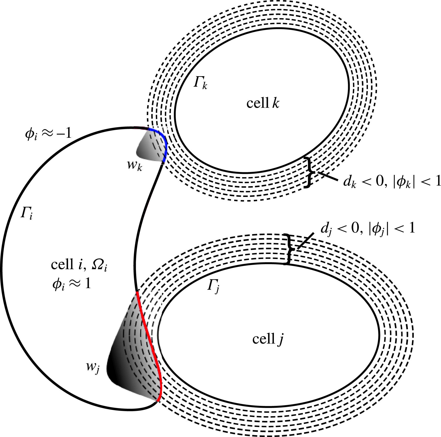
Figure 1 gives a schematic illustration of the interaction terms. The algorithm considers only these cells, for which the diffuse interfaces overlap. All other cells do not contribute to the interaction. In addition, the most expensive part, computing the distance between cells, has been avoided, as this information is already contained in the phase field description of the cells. The approach thus scales with
 $n$
, the number of cells. Similar ideas to model interactions within phase field approaches have been considered in Zhang, Das & Du (Reference Zhang, Das and Du2009) and Gu, Wang & Gunzburger (Reference Gu, Wang and Gunzburger2014). However, only for the interaction of one cell with a fixed substrate.
The red and blue coloured parts of
 ${\it\Gamma}_{i}$
are in contact with the interfaces of cell
 $j$
and cell
 $k$
(dashed contours around those cells), where the signed functions
 $r_{j}$
and
 $r_{k}$
can be calculated and thus also the interaction functions
 $w_{j}$
and
 $w_{k}$
. They do not vanish in the overlapping regions.

The non-dimensional Navier–Stokes equation reads
 $$\begin{eqnarray}\displaystyle & \displaystyle {\it\rho}(\partial _{t}\boldsymbol{v}+\boldsymbol{v}\boldsymbol{\cdot }\boldsymbol{{\rm\nabla}}\boldsymbol{v})+\boldsymbol{{\rm\nabla}}p-\frac{1}{\mathit{Re}}\boldsymbol{{\rm\nabla}}\boldsymbol{\cdot }({\it\nu}\unicode[STIX]{x1D63F})=\mathop{\sum }_{i=1}^{n}{\it\phi}_{i}^{\sharp }\boldsymbol{{\rm\nabla}}{\it\phi}_{i}, & \displaystyle\end{eqnarray}$$
 $$\begin{eqnarray}\displaystyle & \boldsymbol{{\rm\nabla}}\boldsymbol{\cdot }\boldsymbol{v}=0, & \displaystyle\end{eqnarray}$$
with
 ${\it\rho}=1$
and
 ${\it\nu}=(1-{\it\phi}_{\mathit{cell}}/2)+\sum _{i=1}^{n}({\it\nu}_{i}/{\it\nu}_{0})(({\it\phi}_{i}+1)/2)$
. Different densities could be handled in a similar way but are omitted here for simplicity.
To enforce the local inextensibility constraint for the RBCs, we follow the approach of model B in Aland et al. (Reference Aland, Egerer, Lowengrub and Voigt2014). The nonlinear evolution equations for
 ${\it\phi}_{i}$
remain, only the Navier–Stokes equation has to be extended and now reads
 $$\begin{eqnarray}\displaystyle & \displaystyle {\it\rho}(\partial _{t}\boldsymbol{v}+\boldsymbol{v}\boldsymbol{\cdot }\boldsymbol{{\rm\nabla}}\boldsymbol{v})+\boldsymbol{{\rm\nabla}}p-\frac{1}{\mathit{Re}}\boldsymbol{{\rm\nabla}}\boldsymbol{\cdot }({\it\nu}\unicode[STIX]{x1D63F})=\mathop{\sum }_{i=1}^{n}{\it\phi}_{i}^{\sharp }\boldsymbol{{\rm\nabla}}{\it\phi}_{i}+\boldsymbol{{\rm\nabla}}\boldsymbol{\cdot }\left(\frac{|\boldsymbol{{\rm\nabla}}{\it\phi}_{RBCs}|}{2}\unicode[STIX]{x1D64B}{\it\lambda}_{\mathit{local}}\right)\!,\quad & \displaystyle\end{eqnarray}$$
 $$\begin{eqnarray}\displaystyle & \boldsymbol{{\rm\nabla}}\boldsymbol{\cdot }\boldsymbol{v}=0, & \displaystyle\end{eqnarray}$$
with a Lagrange multiplier
 ${\it\lambda}_{\mathit{local}}$
for which we introduce the additional equation
 $$\begin{eqnarray}{\it\xi}{\it\epsilon}^{2}\boldsymbol{{\rm\nabla}}\boldsymbol{\cdot }({\it\phi}_{RBCs}^{2}\boldsymbol{{\rm\nabla}}{\it\lambda}_{\mathit{local}})+\frac{|\boldsymbol{{\rm\nabla}}{\it\phi}_{RBCs}|}{2}\unicode[STIX]{x1D64B}\boldsymbol{ : }\boldsymbol{{\rm\nabla}}\boldsymbol{v}=0,\end{eqnarray}$$
with
 ${\it\xi}>0$
a parameter independent of
 ${\it\epsilon}$
. For
 ${\it\epsilon}\rightarrow 0$
we obtain
 ${\rm\Delta}{\it\lambda}_{\mathit{local}}=0$
away from
 ${\it\Gamma}_{RBCs}$
and
 $\unicode[STIX]{x1D64B}\boldsymbol{ : }\boldsymbol{{\rm\nabla}}\boldsymbol{v}=\boldsymbol{{\rm\nabla}}_{\!{\it\Gamma}}\boldsymbol{\cdot }\boldsymbol{v}=0$
near
 ${\it\Gamma}_{RBCs}$
, which was shown in Aland et al. (Reference Aland, Egerer, Lowengrub and Voigt2014) for
 $n=1$
.
2.4. Thermodynamic consistency
The proposed system of equations (2.12) and (2.13) for
 $i=1,\ldots ,n$
and (2.23) and (2.24) or (2.25)–(2.27) fulfill thermodynamic consistency. To show this, we consider the kinetic energy
 $\mathscr{E}_{kin}=\int \boldsymbol{v}^{2}$
with constant density
 ${\it\rho}=1$
and the cell energy
 $\mathscr{E}$
and show that the time derivative is less than or equal to zero:
 $$\begin{eqnarray}\displaystyle \dot{\mathscr{E}}_{tot}(\boldsymbol{v},{\it\phi}_{1},\ldots ,{\it\phi}_{n})=\dot{\mathscr{E}}_{kin}+\dot{\mathscr{E}}=\int \boldsymbol{v}\boldsymbol{v}_{t}+\mathop{\sum }_{i=1}^{n}{\it\phi}_{i}^{\natural }\partial _{t}{\it\phi}_{i}\,\text{d}\boldsymbol{x}, & & \displaystyle\end{eqnarray}$$
with
 $$\begin{eqnarray}\displaystyle & \partial _{t}{\it\phi}_{i}=-\boldsymbol{v}\boldsymbol{\cdot }\boldsymbol{{\rm\nabla}}{\it\phi}_{i}+{\it\gamma}{\rm\Delta}{\it\phi}_{i}^{\natural }, & \displaystyle\end{eqnarray}$$
 $$\begin{eqnarray}\displaystyle & \displaystyle \partial _{t}\boldsymbol{v}=-(\boldsymbol{v}\boldsymbol{\cdot }\boldsymbol{{\rm\nabla}})\boldsymbol{v}-\boldsymbol{{\rm\nabla}}p+\frac{1}{\mathit{Re}}\boldsymbol{{\rm\nabla}}\boldsymbol{\cdot }({\it\nu}\unicode[STIX]{x1D63F})+\mathop{\sum }_{i=1}^{n}{\it\phi}_{i}^{\sharp }\boldsymbol{{\rm\nabla}}{\it\phi}_{i}+\boldsymbol{{\rm\nabla}}\boldsymbol{\cdot }\left(\frac{|\boldsymbol{{\rm\nabla}}{\it\phi}_{RBCs}|}{2}\unicode[STIX]{x1D64B}{\it\lambda}_{\mathit{local}}\right)\!,\qquad & \displaystyle\end{eqnarray}$$
which yields
 $$\begin{eqnarray}\displaystyle & & \displaystyle \dot{\mathscr{E}}_{tot}(\boldsymbol{v},{\it\phi}_{1},\ldots ,{\it\phi}_{n})\nonumber\\ \displaystyle & & \displaystyle \quad =\int \boldsymbol{v}\boldsymbol{\cdot }\left(-(\boldsymbol{v}\boldsymbol{\cdot }\boldsymbol{{\rm\nabla}})\boldsymbol{v}-\boldsymbol{{\rm\nabla}}p+\frac{1}{\mathit{Re}}\boldsymbol{{\rm\nabla}}\boldsymbol{\cdot }({\it\nu}\unicode[STIX]{x1D63F})+\mathop{\sum }_{i=1}^{n}{\it\phi}_{i}^{\sharp }\boldsymbol{{\rm\nabla}}{\it\phi}_{i}+\boldsymbol{{\rm\nabla}}\boldsymbol{\cdot }\left(\frac{|\boldsymbol{{\rm\nabla}}{\it\phi}_{RBCs}|}{2}\unicode[STIX]{x1D64B}{\it\lambda}_{\mathit{local}}\right)\right)\nonumber\\ \displaystyle & & \displaystyle \qquad +\,\mathop{\sum }_{i=1}^{n}{\it\phi}_{i}^{\natural }(-\boldsymbol{v}\boldsymbol{\cdot }\boldsymbol{{\rm\nabla}}{\it\phi}_{i}+{\it\gamma}{\rm\Delta}{\it\phi}_{i}^{\natural })\,\text{d}\boldsymbol{x}\quad (\text{partial integration, use }\boldsymbol{{\rm\nabla}}\boldsymbol{\cdot }\boldsymbol{v}=0)\nonumber\\ \displaystyle & & \displaystyle \quad =\int -\frac{1}{\mathit{Re}}|\boldsymbol{{\rm\nabla}}\boldsymbol{v}|^{2}-{\it\gamma}\mathop{\sum }_{i=1}^{n}|\boldsymbol{{\rm\nabla}}{\it\phi}_{i}^{\natural }|^{2}-\left(\boldsymbol{{\rm\nabla}}\boldsymbol{v}\boldsymbol{ : }\frac{|\boldsymbol{{\rm\nabla}}{\it\phi}_{RBCs}|}{2}\unicode[STIX]{x1D64B}\right){\it\lambda}_{\mathit{local}}\,\text{d}\boldsymbol{x}\nonumber\\ \displaystyle & & \displaystyle \qquad (\text{use (2.27) and partial integration})\nonumber\\ \displaystyle & & \displaystyle \quad =\int -\frac{1}{\mathit{Re}}|\boldsymbol{{\rm\nabla}}\boldsymbol{v}|^{2}-{\it\gamma}\mathop{\sum }_{i=1}^{n}|\boldsymbol{{\rm\nabla}}{\it\phi}_{i}^{\natural }|^{2}-{\it\xi}{\it\epsilon}^{2}{\it\phi}_{RBCs}^{2}|\boldsymbol{{\rm\nabla}}{\it\lambda}_{\mathit{local}}|^{2}\,\text{d}\boldsymbol{x}\nonumber\\ \displaystyle & & \displaystyle \quad \leqslant 0,\end{eqnarray}$$
where we have used the identity
 $\boldsymbol{v}\times (\boldsymbol{{\rm\nabla}}\times \boldsymbol{v})=\boldsymbol{{\rm\nabla}}(|\boldsymbol{v}|^{2})-(\boldsymbol{v}\boldsymbol{\cdot }\boldsymbol{{\rm\nabla}})\boldsymbol{v}$
from which follows that
 $\int \boldsymbol{v}\boldsymbol{\cdot }(-\boldsymbol{v}\boldsymbol{\cdot }\boldsymbol{{\rm\nabla}}\boldsymbol{v})=0$
.
2.5. Numerical approach
Time discretization. In order to discretize in time, we explore an operator splitting approach. In an iterative process, we first solve the flow problem and substitute its solution into the phase-field equations, which are then solved separately with a parallel splitting method. We split the time interval
 $I=[0,T]$
into equidistant time instants
 $0=t_{0}<t_{1}<\cdots \,$
and define the time steps
 ${\it\tau}:=t_{n+1}-t_{n}$
. Of course, adaptive time steps may also be used. We define the discrete time derivative
 $\text{d}_{t}\cdot ^{n+1}:=(\cdot ^{n+1}-\cdot ^{n})/{\it\tau}$
, where the upper index denotes the time step number and e.g.
 $\boldsymbol{v}^{n}:=\boldsymbol{v}(t_{n})$
is the value of
 $\boldsymbol{v}$
at time
 $t_{n}$
. For each system, a semi-implicit time discretization is used, which together with an appropriate linearization of the involved nonlinear terms leads to a set of linear systems in each time step.
Space discretization. We apply the finite element method to discretize in space, where a
 $P^{2}/P^{1}$
Taylor–Hood element is used for the flow problem, all other quantities are discretized in space using
 $P^{2}$
elements. In each time step we solve the following.
-
(i) The flow problem for
 $\boldsymbol{v}^{n+1}$
,
$p^{n+1}$
and
${\it\lambda}_{\mathit{local}}^{n+1}$
(2.32)
$$\begin{eqnarray}\displaystyle \text{d}_{t}\boldsymbol{v}^{n+1}+(\boldsymbol{v}^{n}\boldsymbol{\cdot }\boldsymbol{{\rm\nabla}})\boldsymbol{v}^{n+1} & = & \displaystyle -\boldsymbol{{\rm\nabla}}p^{n+1}+\frac{1}{\mathit{Re}}\boldsymbol{{\rm\nabla}}\boldsymbol{\cdot }({\it\nu}^{n}\unicode[STIX]{x1D63F}^{n+1})\nonumber\\ \displaystyle & & \displaystyle +\,\mathop{\sum }_{i=1}^{n}{{\it\phi}_{i}^{\natural }}^{n}\boldsymbol{{\rm\nabla}}{\it\phi}_{i}^{n}+\boldsymbol{{\rm\nabla}}\boldsymbol{\cdot }\left(\frac{|\boldsymbol{{\rm\nabla}}{\it\phi}_{RBCs}^{n}|}{2}\unicode[STIX]{x1D64B}^{n}{\it\lambda}_{\mathit{local}}^{n+1}\right)\!,\end{eqnarray}$$
(2.33)
$$\begin{eqnarray}\displaystyle & \boldsymbol{{\rm\nabla}}\boldsymbol{\cdot }\boldsymbol{v}^{n+1}=0, & \displaystyle\end{eqnarray}$$
(2.34)where
$$\begin{eqnarray}\displaystyle & \displaystyle {\it\xi}{\it\epsilon}^{2}\boldsymbol{{\rm\nabla}}\boldsymbol{\cdot }(({\it\phi}_{RBCs}^{n})^{2}\boldsymbol{{\rm\nabla}}{\it\lambda}_{\mathit{local}}^{n+1})+\frac{|\boldsymbol{{\rm\nabla}}{\it\phi}_{RBCs}^{n}|}{2}\unicode[STIX]{x1D64B}^{n}\boldsymbol{ : }\boldsymbol{{\rm\nabla}}\boldsymbol{v}^{n+1}=0, & \displaystyle\end{eqnarray}$$
${\it\nu}^{n}={\it\nu}({\it\phi}^{n})$
and
$\unicode[STIX]{x1D64B}^{n}=\unicode[STIX]{x1D644}-(\boldsymbol{{\rm\nabla}}{\it\phi}^{n}\otimes \boldsymbol{{\rm\nabla}}{\it\phi}^{n}/|\boldsymbol{{\rm\nabla}}{\it\phi}^{n}|^{2})$
.
-
(ii) The phase field equations for
${\it\phi}_{i}^{n+1}$
,
$i=1,\ldots ,n$
(2.35)
$$\begin{eqnarray}\text{d}_{t}{\it\phi}_{i}^{n+1}+\boldsymbol{v}^{n+1}\boldsymbol{\cdot }\boldsymbol{{\rm\nabla}}{\it\phi}_{i}^{n+1}={\it\gamma}{\rm\Delta}{{\it\phi}_{i}^{\natural }}^{n+1},\end{eqnarray}$$
(2.36)
$$\begin{eqnarray}\displaystyle {{\it\phi}_{i}^{\natural }}^{n+1} & = & \displaystyle \frac{1}{\mathit{Re}\,\mathit{Be}_{i}}{\it\psi}_{i}^{n+1}+\frac{c_{i}}{\mathit{Re}\,\mathit{Be}_{i}}(\mathscr{A}_{0,i}-\mathscr{A}({\it\phi}_{i}^{n})){\it\kappa}_{i}^{n}\nonumber\\ \displaystyle & & \displaystyle +\,\frac{1}{\mathit{Re}\,\mathit{In}}\left(B^{\prime }({\it\phi}_{i}^{n})\mathop{\sum }_{\substack{ j=1 \\ j\neq i}}^{n}w_{j}^{n}+{w_{i}^{\prime }}^{n}\mathop{\sum }_{\substack{ j=1 \\ j\neq i}}^{n}B({\it\phi}_{j}^{n})\right)\!,\end{eqnarray}$$
(2.37)
$$\begin{eqnarray}\displaystyle & \displaystyle {\it\psi}_{i}^{n+1}={\rm\Delta}{\it\mu}_{i}^{n+1}-\frac{1}{{\it\epsilon}^{2}}(3({\it\phi}_{i}^{n+1})^{2}+2H_{0}{\it\phi}_{i}^{n+1}-1){\it\mu}_{i}^{n+1}, & \displaystyle\end{eqnarray}$$
(2.38)with
$$\begin{eqnarray}\displaystyle & \displaystyle {\it\mu}_{i}^{n+1}={\it\epsilon}{\rm\Delta}{\it\phi}_{i}^{n+1}-\frac{1}{{\it\epsilon}}(({\it\phi}_{i}^{n+1})^{2}-1)({\it\phi}_{i}^{n+1}+H_{0}), & \displaystyle\end{eqnarray}$$
${\it\kappa}_{i}^{n}=-{\it\epsilon}{\rm\Delta}{\it\phi}_{i}^{n}+(1/{\it\epsilon})(({\it\phi}_{i}^{n})^{2}-1){\it\phi}_{i}^{n}$
. We linearize the nonlinear terms by a Taylor expansion of order one, e.g.
$(({\it\phi}_{i}^{n+1})^{2}-1){\it\phi}_{i}^{n+1}=(({\it\phi}_{i}^{n})^{2}-1){\it\phi}_{i}^{n}+(3({\it\phi}_{i}^{n})^{2}-1)$
$({\it\phi}_{i}^{n+1}-{\it\phi}_{i}^{n})$
.








Implementation. The fully discretized system of partial differential equations is implemented using the adaptive finite element toolbox AMDiS (Vey & Voigt Reference Vey and Voigt2007; Witkowski et al.
Reference Witkowski, Ling, Praetorius and Voigt2015). We use an adaptively refined triangular mesh
 $\mathscr{T}_{h}$
with a high resolution along the cell membranes to guarantee at least five grid points across the diffuse interface. We further conduct a shared memory OPENMP parallelization, to solve the phase field evolutions via a parallel splitting method. Each linear system of equations is solved using the direct unsymmetric multifrontal method UMFPACK. For more details we refer to Ling et al. (Reference Ling, Marth, Praetorius and Voigt2015).
3. Results and discussion
We study WBC margination for different WBC stiffnesses, different haematocrit values and different Reynolds numbers. We consider a blood vessel of thickness
 $20~{\rm\mu}\text{m}$
and length
 $40~{\rm\mu}\text{m}$
with periodic conditions on the inflow and outflow. The relatively small length results from compromising computational efficiency and physical accuracy and has been obtained through detailed investigations on the influence of the periodicity on WBC margination. We consider RBCs with perimeter
 $22~{\rm\mu}\text{m}$
, area
 $19.5~{\rm\mu}\text{m}^{2}$
, bending rigidity
 $b_{N,RBC}=2\times 10^{-19}~\text{J}$
, viscosity
 ${\it\nu}_{RBC}=1\times 10^{-3}~\text{Pa}~\text{s}$
. WBCs are initially set to be circular with a radius of
 $5~{\rm\mu}\text{m}$
. They have a viscosity
 ${\it\nu}_{WBC}=50\times 10^{-2}~\text{Pa}~\text{s}$
. In order to study the influence of the stiffness of the WBCs, we consider three types: soft WBCs with
 $b_{N,WBC}=2\times 10^{-19}~\text{J}$
, hard WBCs with
 $b_{N,WBC}=2\times 10^{-18}~\text{J}$
and rigid WBCs. The interaction strength is constant between all cell types and reads
 ${\it\alpha}=4.24\times 10^{-7}~\text{N}~\text{m}^{-1}$
. For the fluid phase, we consider the viscosity
 ${\it\nu}_{0}=1\times 10^{-3}~\text{Pa}~\text{s}$
. We consider a constant flow rate, which is realized by applying a time-dependent force term
 $\boldsymbol{F}=(1/\mathit{Fr}(t),0)^{\text{T}}$
, where
 $\mathit{Fr}$
denotes the Froude number. If the current flow rate
 $Q(t)$
is lower or greater than the desired flow rate
 $Q_{0}$
, we increase the force term by multiplying it with the ratio of
 $Q_{0}/Q_{t}$
. The initial force term can be estimated from its Newtonian value:
 $1/\mathit{Fr}\;(t=0)=12Q_{0}/(h_{l}^{3}\mathit{Re})$
, where
 $h_{l}$
is the channel height. We choose
 $Q_{0}=15$
for all simulations, which implies an averaged velocity of
 $8.44\times 10^{-5}~\text{m}~\text{s}^{-1}$
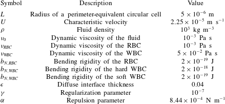
for all simulations and thus allows us to compare the results for different settings. An overview of all used parameters is given in table 1.
Mechanical and numerical parameters used in the simulations. Mechanical parameters correspond to the considered values in Fedosov et al. (Reference Fedosov, Fornleitner and Gompper2012) and Takeishi et al. (Reference Takeishi, Imai, Nakaaki, Yamaguchi and Ishikawa2014).

In non-dimensional units, the computational domain becomes
 ${\it\Omega}=[0,8]\times [0,4]$
, with periodic boundary conditions in the
 $x_{1}$
direction. The WBC has the radius 1 and is put at
 $(5,2)$
. RBCs are placed randomly such that they do not overlap. The non-dimensional numbers read
 $\mathit{Re}=1.125\times 10^{-4}$
,
 $\mathit{Be}_{RBC}=5.3$
,
 $\mathit{Be}_{WBC}=0.53$
(hard),
 $\mathit{Be}_{WBC}=5.3$
(soft),
 $\mathit{In}=0.1$
and
 $\mathit{Fr}(t=0)=4\times 10^{-5}$
. In
 $x_{2}$
direction we specify the Dirichlet conditions
 ${\it\phi}_{i}=-1$
for
 $i=1,\ldots ,n$
, which ensures that all cells stay within the computational domain.
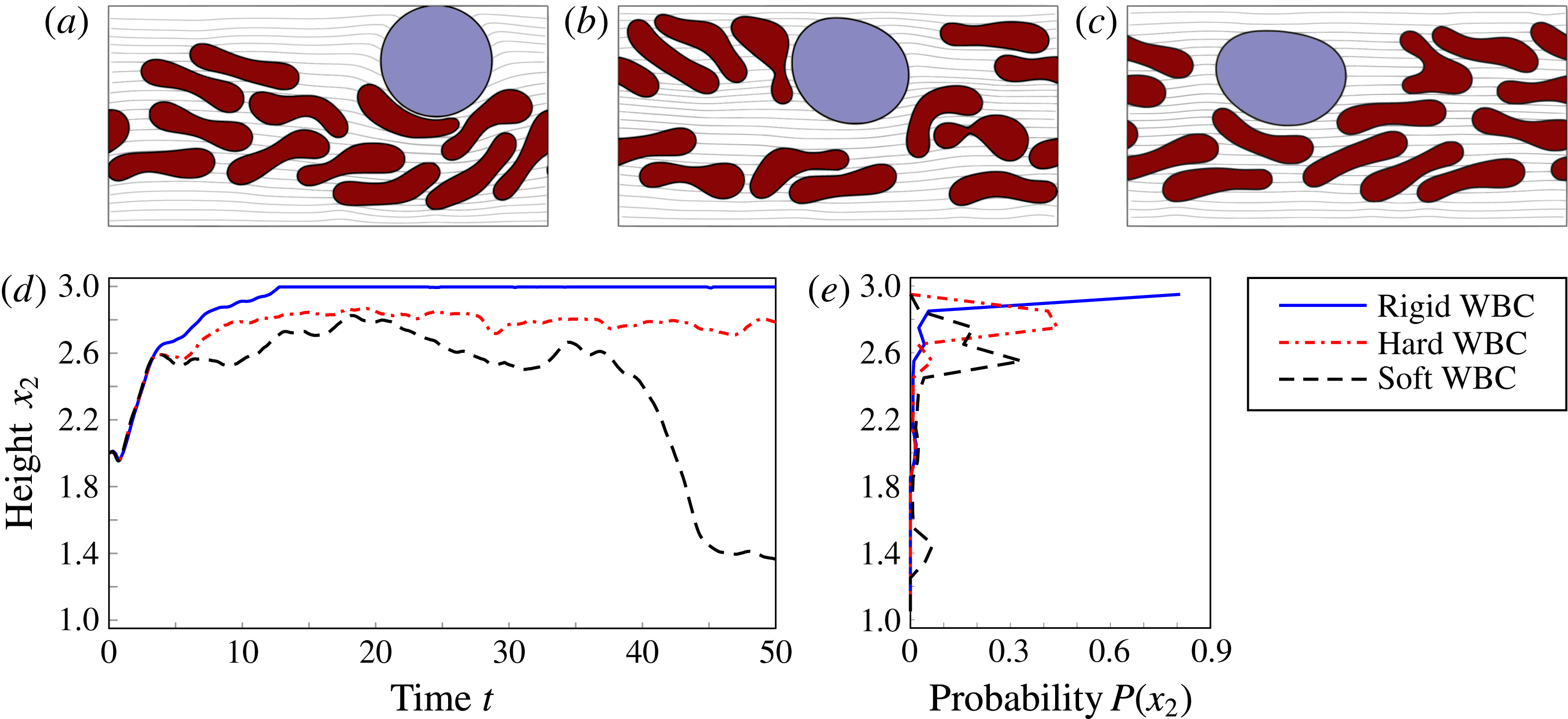
We first vary the deformability of the WBC and keep
 $H_{t}=0.293$
constant. The results are presented in figure 2, where the lower left diagram shows the
 $x_{2}$
coordinate of the trajectory of the midpoint of the WBC. After an initial phase, the WBC moves towards the wall, but only the rigid WBC can attach to the wall, while the soft WBC moves away after a certain time. The lower right diagram shows the probability that the midpoint of the cell is within the upper part of the channel with height 0.1. The results nicely confirm the findings in Fedosov et al. (Reference Fedosov, Fornleitner and Gompper2012), that WBC margination is high for rigid cells and decreases for softer cells.
Simulation snapshot at late time for
 $H_{t}=0.293$
for rigid, hard and soft WBC (a–c),
 $x_{2}$
coordinate for the trajectory of the midpoint of the WBC (e) and the probability that the midpoint of the WBC is inside a defined interval (d). The
 $x_{2}$
axis is split into 20 intervals of length 0.1.

The second test concerns the influence of
 $H_{t}$
. We vary the number of RBCs, which lead to different values of
 $H_{t}$
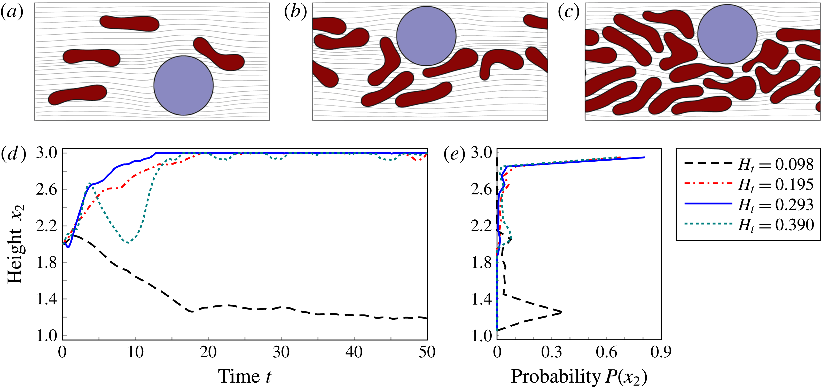
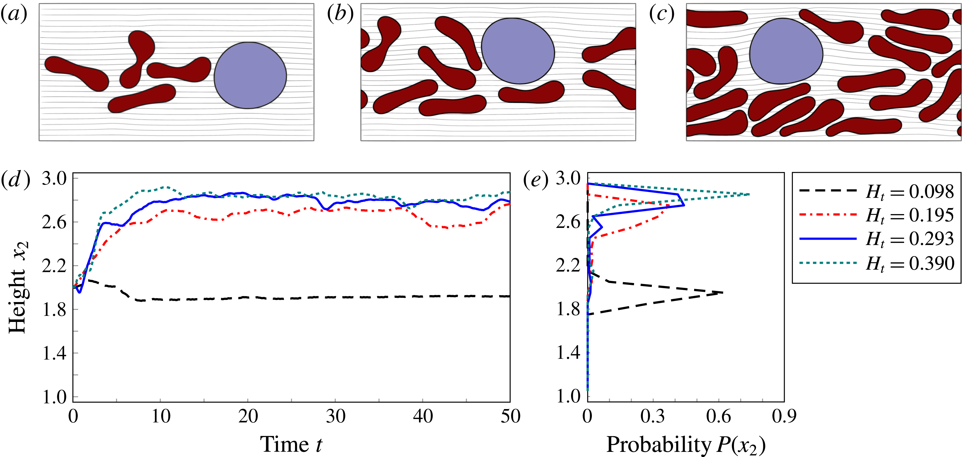
, ranging from 0.098 to 0.39. Figure 3 shows the obtained results for a rigid WBC and figure 4 for a hard one.
Simulation snapshot at late time for a rigid WBC for
 $H_{t}=0.098$
,
 $H_{t}=0.195$
and
 $H_{t}=0.39$
(a–c) (
 $H_{t}=0.293$
is shown in figure 2). The
 $x_{2}$
coordinate for the trajectory of the midpoint of the WBC (e) and the probability that the midpoint of the WBC is inside a defined interval (d). The
 $x_{2}$
axis is split into 20 intervals of length 0.1.

Simulation snapshot at late time for a hard WBC for
 $H_{t}=0.098$
,
 $H_{t}=0.195$
and
 $H_{t}=0.39$
(a–c) (
 $H_{t}=0.293$
is shown in figure 2). The
 $x_{2}$
coordinate for the trajectory of the midpoint of the WBC (e) and the probability that the midpoint of the WBC is inside a defined interval (d). The
 $x_{2}$
axis is split into 20 intervals of length 0.1.

For a rigid WBC, margination can be observed for all considered
 $H_{t}$
. However, our simulations show a lower tendency to move to the wall for the smallest value of
 $H_{t}=0.098$
and the largest tendency for
 $H_{t}=0.195$
and
 $H_{t}=0.293$
. For the highest value
 $H_{t}=0.39$
, the probability slightly decreases. It seems more likely that due to the larger number of RBCs, interaction between WBC and RBCs are also possible close to the wall, which moves the WBC away from the wall, see
 $t=10$
,
 $t=22$
and
 $t=30$
. This results give evidence for a decreasing WBC margination for high
 $H_{t}$
, as also observed in Fedosov et al. (Reference Fedosov, Fornleitner and Gompper2012). In the case of a hard WBC, the cell remains in the centre and in contrast to figure 3, no margination occurs for the lowest
 $H_{t}$
considered. Increasing
 $H_{t}$
leads to WBC margination. However, contact with the wall cannot be achieved. We also do not see the tendency for decreasing WBC margination for
 $H_{t}=0.39$
. Further increasing
 $b_{N,WBC}$
or
 $H_{t}$
is not possible due to numerical reasons.
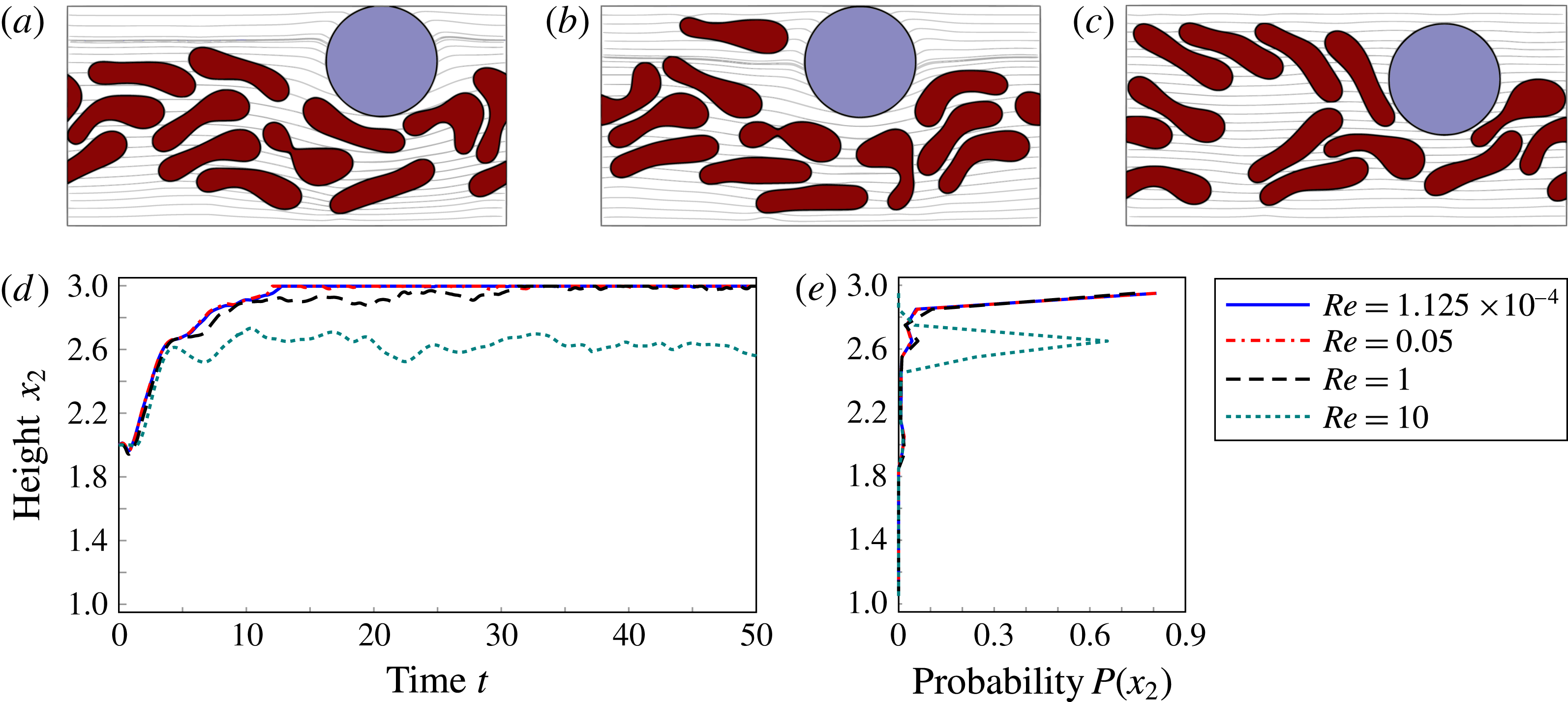
So far, only already known results have been reproduced by the hydrodynamic phase field model, which can be viewed as a validation of the modelling approach. We now turn to the effect of the Reynolds number on WBC margination. It is shown in figure 5. We consider
 $H_{t}=0.293$
and a rigid WBC. Considering a constant flow rate, we obtain WBC margination for
 $\mathit{Re}=1.125\times 10^{-4}$
,
 $\mathit{Re}=0.05$
and
 $\mathit{Re}=1$
. However, the tendency to adhere entirely decreases already for
 $\mathit{Re}=1$
. The simulation results for
 $\mathit{Re}=10$
indicate no margination.
Simulation snapshot at late time for a rigid WBC and
 $H_{t}=0.293$
for
 $\mathit{Re}=0.05$
,
 $\mathit{Re}=1$
and
 $\mathit{Re}=10$
(a–c) (
 $\mathit{Re}=1.125\times 10^{-4}$
is shown in figure 2). The
 $x_{2}$
coordinate for the trajectory of the midpoint of the WBC (e) and the probability that the midpoint of the WBC is inside a defined interval (d). The
 $x_{2}$
axis is split into 20 intervals of length 0.1. For
 $\mathit{Re}=0.05$
a movie is provided in the online supplementary material available at http://dx.doi.org/10.1017/jfm.2016.15.

Various explanations can be given. First, the tendency of RBCs to aggregate in the centre of the vessel might decrease with increasing
 $\mathit{Re}$
due to the increased hydrodynamic interactions. This would increase the concentration of RBCs near the wall and thus lead to a stronger interaction with marginated WBCs, which, similar to the situation for large
 $H_{t}$
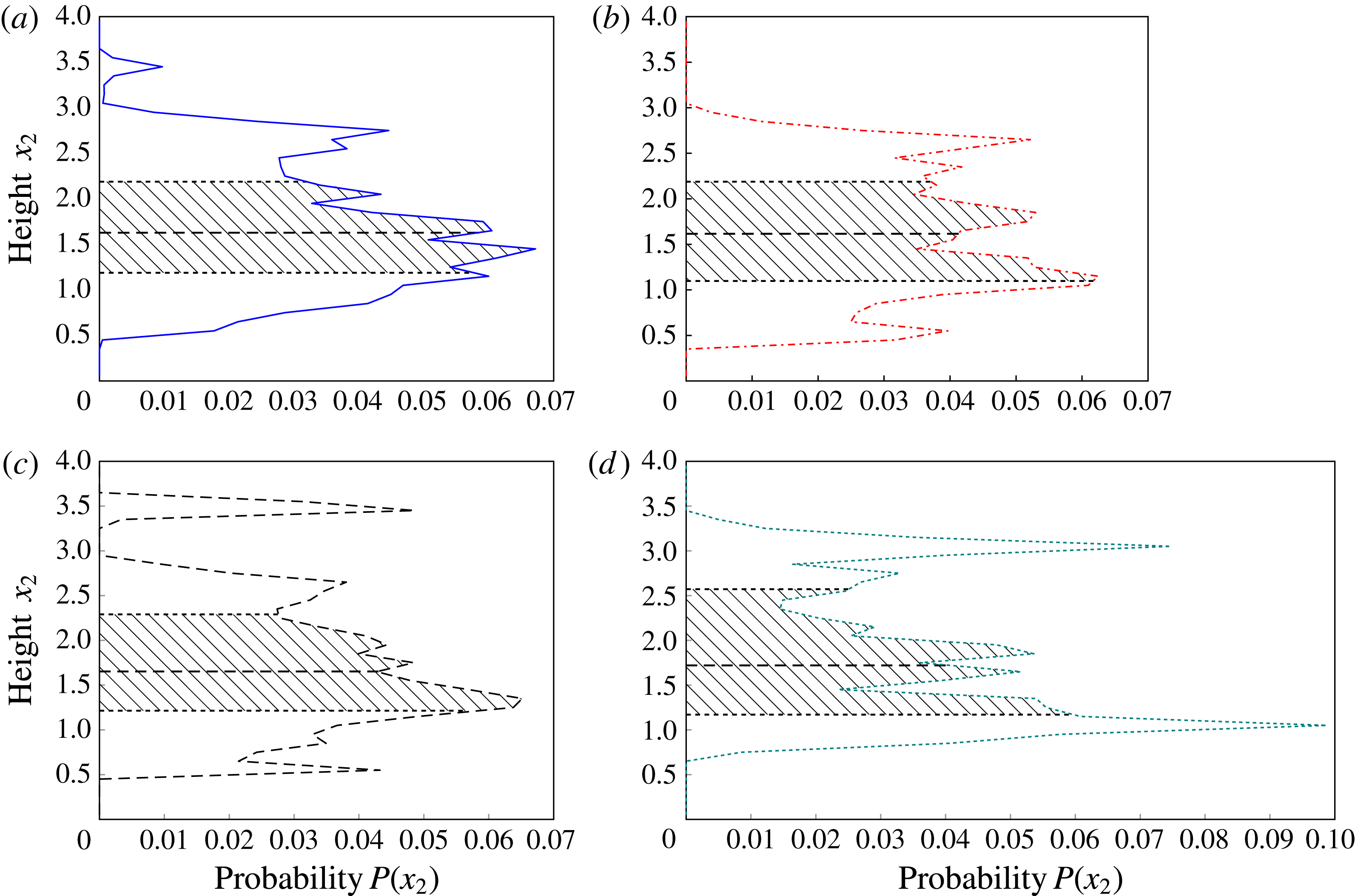
, limits the time WBCs spend near the wall. However, this explanation cannot be justified by our numerical results. Figure 6 shows the distribution of RBCs in the vessel averaged over the simulation time, which does not, or only very weakly show a dependency on
 $\mathit{Re}$
. The median is shifted towards the lower part due to the presence of the WBC in the upper part. The peak in the distribution for
 $\mathit{Re}=1$
and
 $\mathit{Re}=10$
in the upper part close to the wall results from RBCs, which are trapped behind the WBC, see figure 5. The lower half of the vessel thus gives a clearer description of the distribution, with no clear dependency on
 $\mathit{Re}$
. This is in agreement with the results of Krüger, Kaoui & Harting (Reference Krüger, Kaoui and Harting2014), where a qualitative similar distribution profile is observed for a suspension of soft capsules. Up to
 $\mathit{Re}=50$
the profile shows no dependency on
 $\mathit{Re}$
, but for larger
 $\mathit{Re}$
the soft capsules are even strongly concentrated in the central region.
Distribution of RBCs for different
 $\mathit{Re}$
, (a)
 $1.125\times 10^{-4}$
, (b) 0.05, (c) 1 and (d) 10, computed over the time interval
 $t=10$
to
 $t=50$
. The shaded region shows the interquartile range, the difference between the upper and lower quartiles together with the median.

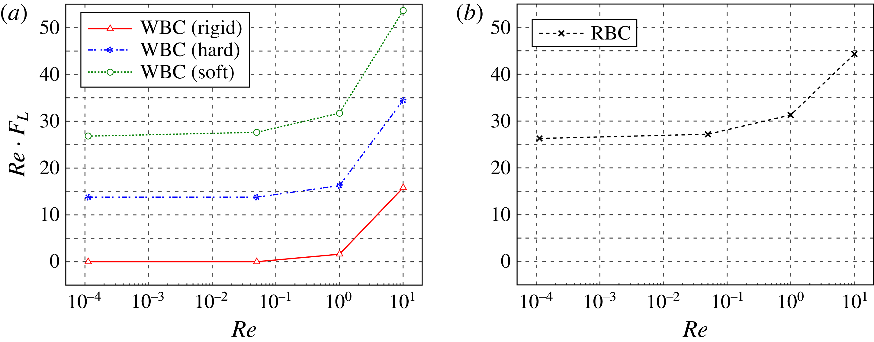
Computed lift force (density) for a WBC (a) and an RBC (b) as a function of
 $\mathit{Re}$
.

The second attempt considered the effect of
 $\mathit{Re}$
on the lift force directly. The investigation of inertial forces on rigid particles dates back to Segre & Silberberg (Reference Segre and Silberberg1961) and its dependency on
 $\mathit{Re}$
is today well understood for spherical objects (Ho & Leal Reference Ho and Leal1974; Schonberg & Hinch Reference Schonberg and Hinch1989; Asmolov Reference Asmolov1999; Matas, Morris & Guazzelli Reference Matas, Morris and Guazzelli2004; Carlo et al.
Reference Carlo, Humphry, Stone and Toner2009). For deformable objects this is much less investigated. Krüger et al. (Reference Krüger, Kaoui and Harting2014) show that the Segre–Silberberg effect is essentially suppressed for deformable objects. We here consider the effect numerically and compute the lift force (density) as a function of
 $\mathit{Re}$
for different cell types. We thereby follow the approach in Meßlinger et al. (Reference Meßlinger, Schmidt, Noguchi and Gompper2009) and adapt a gravitational force
 $\boldsymbol{F}_{g}$
acting on the cell. In the hydrodynamic phase field models (2.23) and (2.25) this is realized by adding
 $-(({\it\phi}_{i}+1)/2)\boldsymbol{F}_{g}$
to the right-hand side. The strength of
 $\boldsymbol{F}_{g}$
is varied to achieve a balance at a fixed height, which is chosen such that the lowest point of the cell is at
 $x_{2}=0.2$
. Due to the strong deformability of the cell the usually used centre of mass position of the cell is not appropriate to achieve comparable results for the same cell type. The magnitude of
 $\boldsymbol{F}_{g}$
now determines the lift force (density) at position
 $x_{2}=0.2$
. Figure 7 shows the computed values for WBCs (considered as rigid, hard and soft cells) and RBCs as a function of
 $\mathit{Re}$
. We observe an increase of the lift force (density) with an increasing
 $\mathit{Re}$
for all cell types. The increase is strongest for the soft WBC. However, also the increase of the lift force for the hard and rigid WBC is significant and explains the decrease in margination for an increasing
 $\mathit{Re}$
, as now both cell types feel a lift force and thus compete for a position away from the vessel wall. However, to quantify this effect is difficult, as the computed values for WBCs and RBCs are not directly comparable, as the actual lift force depends on cell size, viscosity and distance from the vessel wall (Meßlinger et al.
Reference Meßlinger, Schmidt, Noguchi and Gompper2009), which all differ for WBCs and RBCs. However, the larger size of the WBCs and their higher viscosity indicate a stronger increase of the lift force with
 $\mathit{Re}$
if compared with RBCs.
4. Conclusion
We investigate margination of WBCs using a hydrodynamic phase-field approximation of a Helfrich-type curvature-elastic model (Helfrich Reference Helfrich1973). For RBCs various constraints concerning membrane inextensibility and area conservation are considered, while WBCs are modelled using a rigid body approximation or a Helfrich-type curvature model with a weakly extensible membrane. We also consider cell–cell interactions. The fluid flow of the blood plasma and the internal fluids of the cells are modelled using the incompressible Navier–Stokes equations. An idealized two-dimensional blood vessel is used as computational domain.
In the low-
 $\mathit{Re}$
regime we have reproduced previous results, e.g. a decreasing tendency for margination with increasing deformability and a non-monotonic dependency on hematocrit, which quantitatively agree with results of Fedosov et al. (Reference Fedosov, Fornleitner and Gompper2012). Here the non-inertial lift force of WBCs is much lower than that on RBCs, or even zero in the limit of a rigid-body approximation. This results in margination of the WBCs to the RBC-free layer near the wall. With inertia effects the simulations show a decreasing tendency for margination with increasing
 $\mathit{Re}$
. The effect is explained by analysing the lift force on a single WBC and a single RBC as a function of
 $\mathit{Re}$
. We now have an additional inertial lift force, which for all cell types increases if
 $\mathit{Re}$
increases. This is also true for the hard and even the rigid WBC. These forces lead to a competition between WBCs and RBCs for a position away from the vessel wall, which suppresses margination. Due to the huge parameter space, flow confinement, deformability of the WBCs, haematocrit and inertia effects, we had to restrict our simulations to specific combinations, which show the most significant effect on WBC margination.
Acknowledgements
Simulations were carried out at ZIH at TU Dresden and JSC at FZ Jülich. W.M. and A.V. acknowledge support from the German Research Foundation through grant no. Vo-899/11. S.A. acknowledges support from the the German Research Foundation through grant no. Al-1705/1. We further acknowledge support from the European Commission within FP7-PEOPLE-2009-IRSES PHASEFIELD and computing resources at JSC through grant no. HDR06.
Supplementary movie
Supplementary movie is available at http://dx.doi.org/10.1017/jfm.2016.15.