


I. INTRODUCTION
Circular polarization (CP) is often used in satellite communications, as it gives a better cross-polarization for systems with offset parabolic reflectors, despite the associated beam squint [Reference Rudge and Adatia1]. This will result in an increased carrier-to-interference ratio (C/I) for multibeam space applications and a reduced cost for the receiving devices. This polarization is also used when the orientation of a linearly-polarized signal cannot be predicted, or to increase the data rate on a given bandwidth, by using right-handed CP (RHCP) and left-handed CP (LHCP) simultaneously.
However, a high data rate requires a high-gain antenna. The electromagnetic band gap (EBG) antenna [Reference Jackson and Oliner2–Reference Sauleau, Le Ray and Coquet4] constitutes a good candidate to meet the demands for both CP and high gain. Among the various possible applications, this kind of antenna is therefore mainly envisioned for multibeam space communications, on the 29.5–30 GHz frequency band [Reference Chreim5]. The multi-feed EBG antenna is used as a reflector focal feed. Indeed, this antenna can be used to produce overlapped apertures [Reference Chantalat, Thévenot, Monédière, Jecko and Dumon6, Reference Neto, Llombart, Gerini, Bonnedal and De Maagt7], resulting in an efficient multibeam coverage with fewer reflectors on the satellite. Currently, the studied polarization for such antennas is linear polarization (LP), which has to be transformed into a CP for the aforementioned reasons. The first step toward goal is to find the best way to realize a circularly-polarized single horn-fed metallic EBG antenna. Our laboratory has already studied several ways to achieve LP/CP transformation. The next step would be to study a circularly-polarized EBG antenna in the multi-feed case.
This paper presents only the first step in studying the latest developments. However, perspectives and guidelines are also given for the second step. Indeed, the three different solutions are detailed, compared, and a conclusion is given on the best approach to conceive a multi-feed EBG antenna for space applications in the future. The first one involves a self-polarizing EBG material, the second uses a meander-line polarizer (MLP), and the last consists in using a circularly-polarized feed.
The objective is to design a circularly-polarized antenna with a 20 dBi directivity, a boresight axial ratio (AR) lower than 1 dB, and a return loss under −10 dB on the 29.5–30 GHz frequency band which will have the best coverage performance for an envisaged space application.
This article is organized as follows. Section II presents a review on the self-polarizing metallic EBG antenna and on the association of an EBG antenna with an MLP. New theoretical results on the feed-generated CP are described in Section III. The different results are compared in Section IV, which finally concludes on the best solution in the single-feed case, and gives perspectives for a multi-feed EBG antenna.
II. REVIEW ON THE EBG ANTENNA WITH A MLP AND THE SELF-POLARIZING EBG ANTENNA
A) Self-polarizing metallic EBG antenna
In [Reference Arnaud, Chantalat, Monediere, Rodes and Thevenot8], a 20 dBi self-polarizing metallic EBG antenna working around 9 GHz and showing a boresight AR lower than 1 dB over a 100 MHz bandwidth has been conceived, realized and successfully measured (Fig. 1).
View of the manufactured prototype.

This antenna is based on two principles (transmission polarizer and EBG antenna) which are used simultaneously. The EBG material must be partially reflecting and generate a correct polarization at the same time. This partially reflecting material placed over a ground plane then constitutes a resonant cavity. To that end, it will be composed of two layers in the y direction and one in the x direction (Fig. 2). The y-oriented layers are used for both the polarizing and the partially reflecting material, while the x-oriented layer only participates in the partially reflecting material. An incident linearly-polarized plane wave, making a 45° angle with the rods, can be decomposed into two orthogonal components of equal amplitudes, E // and E ⊥. The E // component will be advanced by passing through the polarizer, while the E ⊥ will be left relatively unchanged. It is also necessary to obtain identical EBG reflection coefficients for both field components at the same frequency. By adjusting the self-polarizing EBG material geometry, CP and a partially reflecting material can be obtained.
Definition of the self-polarizing EBG material parameters.

An iris-based matching system has been used to ensure a satisfying return loss, at the cost of a deteriorated AR. A metallic bar (1.2 mm thickness) was then been inserted inside the EBG cavity in order to compensate this degradation and to maintain a perfect LP inside the antenna. The simulated and measured characteristics presented a good agreement.
The purpose of this paper is to compare the different possible designs for a 30 GHz circularly-polarized horn-fed metallic EBG antenna. It is therefore necessary to evaluate the performances of the self-polarizing antenna at 30 GHz. It was done using CST Microwave Studio. The geometrical parameters used for the simulation and the simulated antenna design are defined respectively in Figs 2 and 3.
Vertical cut-plane view of simulated self-polarizing EBG antenna.

Table 1 presents the values of the EBG material parameters as well as the required tolerances. Dimensions of the smooth-walled conical horn and the irises are shown in Figs 4(a–d).
Horn dimensions and geometry and positioning of the irises.

Values of the self-polarizing EBG material parameters.

The antenna is correctly matched over a 200 MHz bandwidth while the desired bandwidth is 500 MHz (Fig. 5). However, it is a very good result for a 23 dBi antenna using this kind of iris. As for all EBG antennas, a reduced directivity would result in an increased matching bandwidth. On the other side, the simulation of the multi-feed EBG antenna shows that it suffers from the mutual coupling between the feeds, which disturb the radiation [Reference Llombart, Neto, Gerini, Bonnedal and De Maagt9]. In [Reference Chreim10], a solution is given to bypass this problem by adding suitable filtering functions at the horn input. In this paper, two concepts have been studied: the unmatched and the matched antenna. The latter decreases the constraints on the required filtering functions and simplifies the design of the whole architecture (antenna and filters). As a conclusion, even if the matching is not perfect, it will help in the case of the multi-feed EBG antenna design. The conclusion is similar for the next cases.
Simulated return loss.

This antenna radiates a LHCP due to the iris orientation. Figure 6 shows the simulated boresight directivity which remains higher than 19 dBi over a 500 MHz bandwidth. To reach 20 dBi, a slight modification of the EBG material would be needed. A simulated boresight AR lower than 1 dB has been obtained over a similar bandwidth (Fig. 6).
Simulated directivity and AR.

The simulated LHCP radiation patterns at 29.7 GHz are quite similar in the different azimuthal cut planes (Fig. 7), and present low sidelobes (<−20 dB). Indeed, a metallic EBG material allows reducing the sidelobe level compared with the dielectric material [Reference Chantalat11]. Figure 8 gives the antenna performances in terms of AR according to the θ-angle. An AR lower than 3 dB is obtained for values of θ between −16° and +16°, which is larger than the half-power beamwidth.
Simulated LHCP radiation patterns in four φ cut planes (29.7 GHz).

Simulated AR in four φ cut planes (29.7 GHz).

B) EBG antenna with MLP
In [Reference Arnaud, Chantalat, Koubeissi, Monediere, Rodes and Thevenot12], the global design of a linearly-polarized metallic EBG antenna with a MLP has been carried out. It resulted in a 24 dBi EBG antenna with a 2.0 dB gain variation and an AR lower than 1 dB on the 29.5–30 GHz frequency band. The EBG material used for this design was a metallic grid with 4 mm holes separated by 4.7 mm, which had been placed 4.56 mm above the ground plane (H cav) [Reference Chantalat13]. The resulting linearly-polarized antenna had been associated with an MLP to obtain the final structure. This MLP was made of two stacked printed-circuit layers, supporting metallic meander lines and has been installed in front of the antenna, at a distance H pol. The layers choice is dictated by an easier manufacturing. The two printed-circuit layers were manufactured using RT Duroid 5880 boards (ɛr = 2.2, 254 µm thickness and 17 µm copper metallization) with one Rohacell layer as spacer (ɛr = 1.1). In [Reference Arnaud, Chantalat, Koubeissi, Monediere, Rodes and Thevenot12], the resulting AR was lower than 1 dB up to 29.7 GHz, frequency beyond which it was disturbed by a resonance occurring between the feeding horn and the EBG grid. This degradation could be simply avoided by reducing the horn longitudinal dimensions and/or by matching the antenna.
The main problem associated with this kind of antenna is the very poor matching. Consequently, a matching device similar to the one used in the first configuration had to be conceived (Figs 9a–c).
Geometry and positioning of the irises.

Another difficulty lies with the number of layers of the polarizer. When the MLP is composed of only two meander-line layers, its reflection coefficient is not negligible. A part of the energy radiated by the antenna will therefore be reflected by the polarizer back into the EBG cavity, which will disturb the existing LP. In turn this will lead to a deteriorated AR for the whole system. As explained before, the insertion of a metallic bar inside the cavity is therefore essential to obtain an AR lower than 1 dB (Fig. 10).
Vertical cut-plane view of simulated EBG antenna associated to the MLP.

The presence of both the iris and the metallic bar slightly deteriorates the AR found in [Reference Arnaud, Chantalat, Koubeissi, Monediere, Rodes and Thevenot12]. Therefore, a new optimization has been made, by changing the value of the T1 and H pol parameters (Fig. 11).
Definition of the MLP parameters.

The final MLP dimensions (mm) are as follow:

As can be seen in Fig. 12, the antenna is matched on a 230 MHz bandwidth, which is similar to the performances of the first antenna.
Simulated return loss.

The simulated boresight directivity, displayed in Fig. 13, remains higher than 20 dBi over a 500 MHz bandwidth, which is a slight improvement over the first solution. On this same band, the AR is lower than 1.2, which is similar to the results obtained with the self-polarizing antenna.
Simulated directivity and AR.

Due to the matching iris orientation, a RHCP is generated, with the radiation pattern exhibiting an axial symmetry (Fig. 14). The sidelobes obtained in the different azimuthal cut planes are moreover, quite low (<−20 dB).
Simulated RHCP radiation patterns in four φ cut planes (29.7 GHz).

The representation of the AR variations over the θ-angle (Fig. 15) shows an equivalent behavior for the two kinds of antennas, i.e. an AR lower than 3 dB for an elevation angle contained between −16° and 16°.
Simulated AR in four φ cut planes (29.7 GHz).

III. HORN GENERATED CP
The last solution consists in obtaining the CP directly, by using a circularly-polarized horn. The latter can be derived from a regular horn either by using a waveguide polarizer or by using two or four coaxial probes as excitation. In both cases, the EBG antenna is presented in Section II.B
A) A waveguide polarizer
CP is defined by two orthogonal field components of equal amplitude with a phase shift of 90° between them. To obtain such characteristics from a linearly-polarized plane wave, one can use a transition presenting a different phase velocity for each field component.
This has first been tried in 1947 by A. Gardner Fox, who installed metallic or dielectric fins in the middle of a circular waveguide [Reference Gardner Fox14]. A fin does not affect the field component perpendicular to it, but the phase velocity of the parallel field component will be diminished. This kind of polarizer was designed empirically, until Ayres gave a calculation method in 1957 [Reference Ayres15]. A sloped or stepped septum can be used instead of the fin, with similar results [Reference Davis, Digiondomenico and Kempic16, Reference Chen and Tsandoulas17].
In our case, and to simplify the simulation, a rectangular waveguide (A = 6.5 mm and B = 5.5 mm) has been placed between two circular-rectangular transition junctions (Figs 16(a) and (b)). The incident wave, linearly polarized and tilted at 45° will be decomposed into two orthogonal components in the circular/rectangular transition. As the dimensions A and B are different, the phase velocity of these two components will also differ. By modifying the length of the rectangular waveguide (L = 1.39 mm), it is possible to adjust the resulting phase shift between the two field components. Figure 17 shows the simulated AR of the waveguide polarizer, which remains lower than 1 dB over the 29.5–30 GHz frequency band.
Simulated waveguide polarizer.

Simulated AR of the waveguide polarizer.

This polarizer can then be installed at the EBG antenna input, before the feeding horn (Fig. 18). A new matching iris, 0.5 mm thickness and designed to allow the propagation of the CP, was placed 0.4 mm below the horn aperture. Its dimensions are shown in Fig. 19.
Vertical cut-plane view of simulated EBG antenna associated to the waveguide polarizer.

The iris dimensions (waveguide polarizer case).

Figure 20 shows the return loss of the EBG antenna without the polarizer. As can be seen, this simple iris induces a correct matching over half of the desired bandwidth.
Simulated return loss of EBG antenna without polarizer.

To obtain a perfect CP, it is necessary for the antenna to be perfectly matched. Otherwise, the field polarization inside the EBG cavity will be the superposition of a LHCP and a RHCP, which will result in an elliptical polarization and a deteriorated AR (Fig. 21).
Simulated AR of EBG antenna with polarizer.

Indeed, the linearly-polarized wave with, for example, a 45° orientation at the polarizer input, is transformed into a circularly polarized one (e.g. LHCP). A part of this wave is transmitted to the antenna and the other part is reflected. The latter is converted back into LP in the polarizer but with a 135° orientation, and is reflected at the waveguide end. This LP with a 135° orientation is transformed into a RHCP by the polarizer. A part of this wave is transmitted to the antenna and another part is reflected. The transmitted part interacts destructively with the LHCP already existing inside the cavity. This effect is more important with a poorly-matched antenna, or one with an already high AR.
Therefore, this kind of polarizer cannot be considered when aiming at an AR lower than 1 dB over a 500 MHz bandwidth. This problem could have been avoided by using a septum polarizer but it is not compatible with a multi-feed EBG antenna, due to its size.
B) Coaxial probes
The last possible approach is to use multiple coaxial probes in order to directly generate a circularly-polarized wave inside the circular waveguide. The simplest configuration requires two coaxial probes, spatially and temporally shifted by 90°, and positioned at λg/4 from the waveguide end.
This configuration does not work properly because of the high coupling between the probes (S 21 > −20 dB), which increases the AR. This coupling, which can be either constructive or destructive, depending on the phase shift between the ports, results in a difference between the E θ and E φ electric field amplitudes. The working of this antenna can be better apprehended by considering two coupled linearly-polarized antennas (Fig. 22).
Schematic diagram of the dual feed horn antenna.

From the article [Reference Drouet, Thevenot and Chantalat18], the two incident waves ( $\overrightarrow {E}$) can be derived from the simplified equation (1), which gives a good estimate of the theoretical AR.
 $$\lpar \overrightarrow {E}\rpar = [ 1+S ] \quad \lpar \overrightarrow {P}\rpar$$
where S is the scattering matrix and  $\overrightarrow {P}$ is the input weight vector.
Equation (1) can also be written as follows:
 $$\left(\matrix{ {E_\theta} \cr {E_\phi} \cr}\right) = \left[1+S\right] \left(\matrix {1\comma \, 0^\circ \cr 1\comma \, 90^\circ } \right)$$
It is therefore beneficial to add a guided wavelength (λg) between the coaxial probes (Fig. 23a), which will decrease the mutual coupling (S 21 < −50 dB).
Simulated two or four coaxial probes antennas.

The last solution is to use four coaxial probes spatially and temporally-shifted by 90° but placed in the same z-plane (Fig. 23b).
This configuration eliminates the coupling between the accesses and thus improves the AR bandwidth. The electric fields E1 and E2, created respectively by the ports 1 and 3, spatially and temporally-shifted by 180°, will add up (Fig. 24). At the opposite, the coupling effects will cancel themselves on these two ports (C1 with C2 and C3 with C4), due to the 180° phase shift. The working is the same for the two other ports.
Principle of the simulated four coaxial probes antenna.

This technique has already been used to improve the AR bandwidth of circularly-polarized microstrip antennas [Reference Kumar and Ray19].
Figure 25 shows the simulated four coaxial probes antenna and Fig. 26 shows the simulated AR of the EBG antenna for the three configurations. The best solution is the one with four probes, as it ensures an AR lower than 1 dB over a wider bandwidth.
Simulated four coaxial probes antenna.

Simulated AR of EBG antenna fed by probes. (a) Two coaxial probes separated by λg. (b) Four coaxial probes. (c) Two coaxial probes on the same plane z.

The second configuration (Fig. 23a), with two probes separated by λg, is also sufficient for this application. The narrower bandwidth obtained in this case is the result of the distance between the probes, being equal to λg at only one frequency. Finally, the first solution with two probes in the same z-plane, results in an AR higher than 1 dB.
Figure 27 presents the new iris, designed for the previous configurations. The resulting performances in terms of return loss are presented in Fig. 28, the matching being almost the same for the different accesses. A correct matching is obtained over the whole bandwidth with a four-port configuration, while only half the band is covered when using only two excitations.
The iris dimensions (feeding probes).

Simulated return losses of EBG antenna fed by probes. (a) Two coaxial probes separated by λg. (b) Four coaxial probes.

The simulated boresight directivity (Fig. 29) is identical in both cases, and similar to the one of the linearly-polarized antenna. Figure 30 shows that the simulated LHCP radiation patterns (29.7 GHz) in the four-probe case are almost identical to each other. The sidelobe level is lower than in the previous configurations (<− 30 dB), due to the lack of parasitic device, such as the MLP. AR values lower than 3 dB can be obtained for elevation angles ranging from −16° to 16°, which is the value obtained in the previous cases (Fig. 31).
Simulated directivity of EBG antenna fed by probes.

Simulated LHCP radiation patterns in four φ cut planes (29.7 GHz).

Simulated AR in four φ cut planes (29.7 GHz).

IV. COMPARISON OF RESULTS FOR THE VARIOUS CONFIGURATIONS AND PERSPECTIVES
Three methods have been studied in this paper to design a 30 GHz circularly-polarized, single horn-fed metallic EBG antenna:
– a self-polarizing metallic EBG antenna,
– an EBG antenna associated to a MLP,
– a circularly-polarized feeding horn.
The best results are obtained with the last configuration in the single-feed EBG antenna case, by using four coaxial probes spatially and temporally shifted by 90°. Using this, a very large 3 dB AR bandwidth can be obtained, with a radiation pattern similar to the one of a linearly polarized antenna. Nevertheless, this impressive result is less significant if the difficulty to create a perfect feeding device, able to work over a large frequency bandwidth, is taken into account.
The solution with two probes separated by λg is easier to achieve, and guarantees a similar amplitude for both field components. However, this solution increases the waveguide length and therefore the antenna size, which will tend to discard this configuration. Moreover, using the horn to transform a LP into a CP will heavily complicate the system in the case of a multi-feed EBG antenna. Indeed the filter design will be much more complex with circularly-polarized horns [Reference Chreim5]. It is better to consider one of the two other alternatives (MLP or self-polarizing material), which would allow the LP of any number of antennas to be transformed into a CP by a single device.
Between these two choices, the best one seems to be the MLP, which separates the partially reflecting EBG material and the polarizing effect, thus greatly easing both the design and the manufacturing. Another advantage of the MLP configuration lies with its years-long use for space applications.
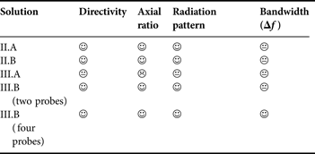
Table 2 summarizes the circularly-polarized EBG antenna performances in the various configurations.
Circularly-polarized EBG antenna performances according to the various configurations.
With the previously presented design, it was necessary to add a metallic bar inside the cavity to ensure an AR lower than 1 dB. This was due to the MLP being made of only two layers, which resulted in a rather high reflection coefficient. An MLP with more layers would present a reduced reflection coefficient [Reference Bhattacharyya and Chwalek20], which would make the metallic bar superfluous.
In this context, an EBG antenna test with a four-layer MLP has been designed. Its working frequency has been decreased to 10 GHz, as well as its directivity (>18 dBi over the bandwidth) to reduce simulation time. Table 3 presents the geometry parameters of the four MLP layers (in mm), which were designed as explained in Section II. The EBG material is a metallic grid with 12.6 mm holes separated by 15.24 mm. The matching device is the iris of the 30 GHz antenna, scaled up to operate at 10 GHz.
Value of four layered MLP parameters.

Figure 32 shows the simulated boresight directivity, which is greater than 18 dBi over a 150 MHz bandwidth, corresponding to a 500 MHz bandwidth at 30 GHz. Without the metallic bar, the simulated AR is lower than 1 dB over the whole bandwidth (Fig. 32), while a good matching is obtained over more than the half bandwidth (Fig. 33).
Simulated directivity and AR.

Simulated return loss.

This confirms this solution as the most appropriate for a multi-feed EBG antenna. Furthermore, the low reflection coefficient of the four-layer MLP will not affect the matching and the coupling between feeds of the multi-feed EGB antenna. Therefore, a good design of a linearly-polarized multi-feed EBG antenna will allow a good circularly-polarized multi-feed EBG antenna design.
V. CONCLUSION
This paper details the different approaches which can be used to design a 30 GHz circularly-polarized single horn-fed metallic EBG antenna. A detailed comparison has been proposed in the realistic case of a 20 dBi EBG antenna with an AR less than 1 dB over a 500 MHz bandwidth. Based on this comprehensive study and on the imperatives of space operation, the authors of this article conclude on the best configuration for a multi-feed EBG antenna, i.e. an EBG antenna with a four-layer MLP.
 Eric Arnaud was born in France in 1970. He received the Diplôme D'Etudes Supérieures Specialisées (DESS) and Ph.D. degrees in Electronics and Telecommunication from the University of Limoges in 1994 and 2010, respectively. He did his Ph.D. on circularly polarized EBG antenna. From 1996 to 2001, he has been in charge of the microwave part of Free-Electron Laser (L.U.R.E). Since 2001, he has been in charge of XLIM laboratory's antenna test range. He participated in several research projects related to the design, development, and characterization of antennas. His research interests are mainly in the fields of circularly polarized EBG antenna and realization of antennas through ink-jetting of conductive inks on RF substrates.
 Regis Chantalat was born in Brive la Gaillarde, France, in 1976. He received the Ph.D. degree in High Frequency Electronics and Optoelectronics from the University of Limoges in 2003. In 2006, he joined the Technology Transfer Center of OSA Department (XLIM laboratory) named Cisteme, as antenna project manager. His activities are focused on the modeling and the design of periodic structures (EBG material, Frequency Selective Surface) and their applications in high gain antennas.
 Thierry Monediere was born in 1964 in Tulle (France). He obtained his Ph.D. in 1990 from the IRCOM Laboratory of the University of Limoges. He is also Professor in the University of Limoges and develops his research activities in XLIM laboratory (UMR CNRS/University of Limoges). He works on multifunction antennas, EBG antennas, and also active antennas.
 Emmanuel Rodes received his Master degree in High Frequency Electronics from the Bordeaux I University, France in 2003 and his Ph.D. from the Limoges University in 2006. Since 2007, he has been an associate professor at the XLIM laboratory in Limoges, France, working first on the design of BIE antennas for various applications. For a few years now, his main field of research has been the improvement of wireless communication through the use of time-reversal.
 Marc Thevenot was born in Limoges, France, in February 1971. He received the B.S. and M.Sc. degrees in microwaves and Doctor Degree in Electronic from the University of Limoges, France, respectively, in 1995, and 1999. In 2001, he joined the National de la Recherche Scientifique (CNRS), Limoges, France. His current research interest is microwave electromagnetism applied to the antenna domain and electromagnetic bandgap (EBG) materials for microwaves.



