1 Introduction
Since the pioneering work of Mack (Reference Mack1984) it is known that three-dimensional oblique instability waves are the most amplified disturbances for a supersonic flat-plate boundary layer (
 $1<M<4$
). Although alternative routes to turbulence cannot be completely ruled out, such three-dimensional oblique waves are most likely initiating the transition process for this Mach number range, leading to so-called ‘oblique breakdown’ (see Thumm, Wolz & Fasel Reference Thumm, Wolz, Fasel, Arnal and Michel1989). Fasel, Thumm & Bestek (Reference Fasel, Thumm, Bestek, Kral and Zang1993) using direct numerical simulation (DNS) and Chang & Malik (Reference Chang and Malik1994) employing parabolized stability equations (PSE) showed that for a flat-plate boundary layer, oblique breakdown may be a relevant transition scenario.
Furthermore, Mayer, Wernz & Fasel (Reference Mayer, Wernz and Fasel2007) performed DNS, adopting a set-up corresponding to the experimental studies by Ermolaev, Kosinov & Semionov (Reference Ermolaev, Kosinov, Semionov, Duck and Hall1996), for a flat plate at Mach 2. These simulations indicate that oblique breakdown may also be present in the experiments by Ermolaev et al. In the nonlinear regime this breakdown mechanism is characterized by the emergence of a nonlinearly generated steady mode with twice the spanwise wavenumber as the primary oblique wave and an unsteady mode with the same frequency as the primary wave but three times the spanwise wavenumber. In particular, the steady mode is considered to be the signature mode of oblique breakdown since it determines the characteristics of the transitional regime. In this publication, the generation and the growth of this steady mode are investigated in great detail and the physical mechanisms responsible for the predominant role of this mode are identified. As transition progresses, higher harmonics of these waves are generated and eventually lead to breakdown to turbulence.
Spatial DNS of the complete transition process of oblique breakdown, covering all stages from the small-amplitude (linear) regime to turbulence were performed by Jiang et al. (Reference Jiang, Choudhari, Chang and Liu2006) and Mayer, von Terzi & Fasel (Reference Mayer, von Terzi and Fasel2010) for a flat plate at Mach 4.5 and 3.0, respectively. They documented the amplitude development of the different modes involved in the transition process, the resulting flow structures, as well as statistical quantities in the transitional/turbulent regime. For a sharp cone under the experimental conditions of Corke, Cavalieri & Matlis (Reference Corke, Cavalieri and Matlis2002), Laible, Mayer & Fasel (Reference Laible, Mayer and Fasel2009) conducted spatial simulations of oblique breakdown and demonstrated that oblique breakdown is also a viable path to turbulence for this geometry and flow conditions. The temporal investigation presented in this publication, is closely related to these spatial simulations, i.e. the boundary and initial conditions are taken from an axisymmetric steady flow calculation of Laible et al. (Reference Laible, Mayer and Fasel2009).
The predominance of the longitudinal mode was also observed in ‘oblique transition’, which is the incompressible scenario that is similar, but not identical, to ‘oblique breakdown’. It is important to first state the fundamental differences between these two transition scenarios before the similarities are pointed out. Oblique transition was proposed by Schmid & Henningson (Reference Schmid and Henningson1992) Berlin, Lundbladh & Henningson (Reference Berlin, Lundbladh and Henningson1994) as a possible mechanism for bypass transition for incompressible boundary layer flows. Instead of initiating oblique waves with a small amplitude, which is the case for oblique breakdown, oblique transition is initiated by a pair of finite-amplitude waves. The consideration behind the two different set-ups is that for supersonic boundary layers, three-dimensional oblique waves are the most amplified waves, and it is therefore reasonable to assume that the exponential growth of these waves may eventually lead to transition. In contrast, for incompressible boundary layers, three-dimensional waves are typically less amplified than two-dimensional waves (see Squire Reference Squire1933). Therefore, based on the exponential growth theory, such three-dimensional waves are not considered to take on the predominant role in the transition process if the initial disturbance spectrum is broad. This may change, however, if the disturbance input and the subsequent receptivity process cause three-dimensional oblique waves to be generated at a significantly higher amplitude level than the two-dimensional waves. One example of such a scenario is a harmonic point source as shown by Stemmer & Kloker (Reference Stemmer and Kloker2000). In their case the initial disturbance development was still exponential and led to a ‘multiple oblique breakdown’ scenario. Similarly to the harmonic point source, an isolated roughness element is considered to generate three-dimensional disturbances at large amplitudes, hence for oblique transition, the flow is perturbed with a large-amplitude oblique disturbance in order to trigger transition. This significant difference in the initialization has important consequences for the transition process. For oblique transition, the primary pair of oblique waves experiences exponential growth only over a short time/distance, if at all, since it is initiated with a high amplitude. In turn, the longitudinal mode is nonlinearly generated at a high amplitude level as well. Directly after its generation, this mode experiences strong growth, which was attributed by Schmid & Henningson (Reference Schmid and Henningson1992) to non-modal or transient growth, and eventually becomes the mode with the highest energy content. In oblique breakdown, on the other hand, the regime where the primary pair of oblique waves is growing exponentially is of significant length. Because the primary pair of oblique waves is initiated at a low amplitude, the longitudinal mode is nonlinearly generated at a low amplitude as well. These differences in the initialization of the transition process have a considerable effect on the flow field, as shown by Kloker & Stemmer (Reference Kloker and Stemmer2003). Whereas due to significant longitudinal vorticity the longitudinal mode in oblique breakdown is appropriately termed a vortex mode, this is typically not the case for the longitudinal mode subject to transient growth in oblique transition. Furthermore, the growth rate of the longitudinal mode is different between the two transition scenarios. In contrast to the non-modal growth experienced in oblique transition, the growth rate of the longitudinal mode is twice as large as the growth rate of the primary pair of oblique waves for oblique breakdown. This suggests that the growth rate is governed by a nonlinear forcing mechanism resulting from the primary pair of oblique waves acting on the longitudinal mode. Although the growth rates are different, Schmid & Henningson (Reference Schmid and Henningson1992) suggested that non-modal growth is also present in oblique breakdown and could explain the predominant role of the longitudinal mode. The objective of this investigation is to (i) explain the underlying physical mechanisms that lead to the dominant role of the longitudinal mode and (ii), if possible, make the connection to incompressible oblique transition.
2 Temporal Navier–Stokes solver
The primary tool used for this investigation is the temporal Navier–Stokes solver described below. The choice of performing the simulations with a temporal rather than a spatial solver is due to the fact that the temporal model significantly simplifies the theoretical analysis of the underlying physical mechanisms in oblique breakdown. In particular, the equations governing the nonlinear interaction of the primary pair of oblique waves would be more complicated for the spatial approach and, more importantly, non-parallel effects inherent in the spatial model would considerably complicate the analysis presented in this paper. It is important to note that although quantitative differences are expected between the spatial and the temporal problem, in many cases, transition phenomena observed in a temporal simulation are qualitatively relevant also to the spatial (physically realistic) case.
2.1 Governing equations
The governing equations for the temporal Navier–Stokes solver are the compressible Navier–Stokes equations in conservative variable formulation for cylindrical coordinates,
 $$\begin{eqnarray}{\displaystyle \frac{\unicode[STIX]{x2202}\boldsymbol{U}}{\unicode[STIX]{x2202}t}}+{\displaystyle \frac{\unicode[STIX]{x2202}(\boldsymbol{E}_{c}+\boldsymbol{E}_{d})}{\unicode[STIX]{x2202}x}}+{\displaystyle \frac{\unicode[STIX]{x2202}(\boldsymbol{F}_{c}+\boldsymbol{F}_{d})}{\unicode[STIX]{x2202}y}}+{\displaystyle \frac{1}{r}}{\displaystyle \frac{\unicode[STIX]{x2202}(\boldsymbol{G}_{c}+\boldsymbol{G}_{d})}{\unicode[STIX]{x2202}\unicode[STIX]{x1D711}}}+{\displaystyle \frac{1}{r}}\boldsymbol{H}+F_{force}=0,\end{eqnarray}$$
where
 $x$
is the downstream coordinate parallel to the cylinder surface,
 $y$
is the wall-normal coordinate orthogonal to the cylinder surface and
 $\unicode[STIX]{x1D711}$
specifies the azimuthal coordinate. The radius,
 $r$
, denotes the local radius,
 $r=y+r_{0}$
, where
 $r_{0}$
is the cylinder radius. We omit stating the well-known vectors for the conservative variables (
 $\boldsymbol{U}$
), the convective fluxes (
 $\boldsymbol{E}_{c},\boldsymbol{F}_{c},\boldsymbol{G}_{c}$
), the viscous terms (
 $\boldsymbol{E}_{d},\boldsymbol{F}_{d},\boldsymbol{G}_{d}$
) and the source term (
 $\boldsymbol{H}$
), but instead refer the interested reader to other publications as e.g. Sandberg & Fasel (Reference Sandberg and Fasel2006). The forcing term (
 $F_{force}$
), which is typically added to the right-hand side, is discussed below.
The set of equations is closed with the equation of state for an ideal gas,
 $$\begin{eqnarray}p={\displaystyle \frac{1}{\unicode[STIX]{x1D6FE}M^{2}}}\unicode[STIX]{x1D70C}T,\end{eqnarray}$$
and the viscosity is calculated using Sutherland’s law,
 $$\begin{eqnarray}\unicode[STIX]{x1D707}=T^{3/2}{\displaystyle \frac{1+{\displaystyle \frac{C}{T_{\infty }^{\ast }}}}{T+{\displaystyle \frac{C}{T_{\infty }^{\ast }}}}},\end{eqnarray}$$
where
 $C=110.4~\text{K}$
and
 $T_{\infty }^{\ast }$
represents the dimensional free-stream temperature. The non-dimensional quantities and parameters in the above equations are defined as
 $$\begin{eqnarray}p={\displaystyle \frac{p^{\ast }}{\unicode[STIX]{x1D70C}_{\infty }^{\ast }U_{\infty }^{\ast 2}}},\quad \unicode[STIX]{x1D70C}={\displaystyle \frac{\unicode[STIX]{x1D70C}^{\ast }}{\unicode[STIX]{x1D70C}_{\infty }^{\ast }}},\quad T={\displaystyle \frac{T^{\ast }}{T_{\infty }^{\ast }}},\quad M={\displaystyle \frac{U_{\infty }^{\ast }}{c_{\infty }^{\ast }}}={\displaystyle \frac{U_{\infty }^{\ast }}{\sqrt{\unicode[STIX]{x1D6FE}p_{\infty }^{\ast }/\unicode[STIX]{x1D70C}_{\infty }^{\ast }}}},\end{eqnarray}$$
with
 $\unicode[STIX]{x1D6FE}$
being the ratio of the specific heats. The subscript
 $_{\infty }$
denotes free-stream values and the superscript
 $^{\ast }$
denotes dimensional quantities.
2.2 Numerical scheme
The Navier–Stokes equations are integrated in time with a standard fourth-order accurate Runge–Kutta scheme. The spatial discretization in the wall-normal/radial direction is based on high-order accurate finite differences. In particular, the wall-normal derivatives of the viscous and source terms are calculated by eighth-order central differences. The inviscid flux in the wall-normal direction is divided into an upwind flux and a downwind flux using van Leer’s splitting (see van Leer Reference van Leer1982). Then, grid-centred upwind differences (see Zhong Reference Zhong1998) with ninth-order accuracy are applied to evaluate the derivatives for these fluxes. These grid-centred upwind differences are derived using the factor
 $\unicode[STIX]{x1D6FC}$
, which prescribes the degree of upwinding,
 $$\begin{eqnarray}{\displaystyle \frac{\unicode[STIX]{x2202}\unicode[STIX]{x1D719}_{j}}{\unicode[STIX]{x2202}y}}=\mathop{\sum }_{k=j-N}^{j+N}c_{k}\unicode[STIX]{x1D719}_{k}-\unicode[STIX]{x1D6FC}_{1}\overline{\unicode[STIX]{x0394}y}{\displaystyle \frac{\unicode[STIX]{x2202}^{2N}\unicode[STIX]{x1D719}_{j}}{\unicode[STIX]{x2202}y^{2N}}}.\end{eqnarray}$$
Hereby
 $\unicode[STIX]{x1D719}_{k}$
denotes the flow variable at the wall-normal grid point index
 $k$
, the values of
 $c_{k}$
are the stencil coefficients and
 $\overline{\unicode[STIX]{x0394}y}$
is the averaged grid spacing over the stencil interval. The parameter
 $N$
determines the number of grid points in the stencil. The ninth-order upwind scheme is derived by setting
 $N=5$
and
 $\unicode[STIX]{x1D6FC}_{1}=-1500$
. Note that for
 $\unicode[STIX]{x1D6FC}_{1}=0$
the upwind scheme reduces to a central difference scheme. Furthermore, all stencil coefficients are derived for a stretched grid.
Special attention is devoted to the wall-next boundary stencils. Since high-order-accurate boundary closures are typically unstable, the present code adopts a method proposed by Zhong & Tatineni (Reference Zhong and Tatineni2003). The basic idea is to stabilize the numerical scheme by using a stretched grid close to the wall. In particular, the following stretching function has the effect to weight the coefficients of the boundary-next stencils such that, on the one hand, the numerical stability is ensured, and that on the other hand, the penalty on the time step requirement of the explicit time-integration scheme is kept at a minimum,
 $$\begin{eqnarray}y(j)={\displaystyle \frac{\arcsin (-\unicode[STIX]{x1D6FC}_{2}\cos (\unicode[STIX]{x03C0}j/2N_{y}))}{\arcsin (\unicode[STIX]{x1D6FC}_{2})}}.\end{eqnarray}$$
Hereby
 $j$
denotes the grid point index in wall-normal direction,
 $N_{y}$
is the total number of grid points in wall-normal direction and the parameter
 $\unicode[STIX]{x1D6FC}_{2}$
determines the degree of grid stretching. This formula is a slight modification of Zhong’s original formula, i.e. stretching is only applied at the wall boundary and not (like in Zhong & Tatineni Reference Zhong and Tatineni2003) at the wall and the free-stream boundary. This is advantageous for boundary layer simulations, since typically a rather strong grid stretching away from the wall has to be employed. Because this technique is not applied at the free stream, an otherwise numerically unstable boundary closure is circumvented by reducing the order of accuracy of the spatial difference stencils at this boundary and the boundary-adjacent points to third-order. Note that for all simulations presented in this publication the free-stream boundary is located sufficiently far away from the wall (
 ${\approx}50\unicode[STIX]{x1D6FF}_{99}$
) so that the order of accuracy at this boundary has a negligible effect on the results. For the streamwise and azimuthal directions, a pseudo-spectral discretization using Fourier modes was adopted (Canuto et al.
Reference Canuto, Hussaini, Quateroni and Zang1988). In particular, the streamwise direction was discretized using both sine and cosine modes whereas the azimuthal direction was discretized with symmetric Fourier modes (
 $\cos$
) for
 $u,v,T,\ldots$
and anti-symmetric Fourier modes (
 $\sin$
) for
 $w$
,
 $\unicode[STIX]{x1D70C}w$
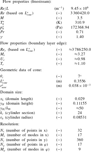
. In order to avoid aliasing errors, the flow variables in physical space are calculated on a sufficient number of collocation points (see table 1). Thus this temporal code is overall of a very high order of accuracy.
Computational parameters.

2.3 Boundary conditions
For temporal simulations, the streamwise direction is assumed to be periodic, i.e.
 $\unicode[STIX]{x1D719}_{x_{L}}=\unicode[STIX]{x1D719}_{x_{0}}$
and
 $\unicode[STIX]{x2202}^{n}\unicode[STIX]{x1D719}/\unicode[STIX]{x2202}x^{n}|_{x_{L}}=\unicode[STIX]{x2202}^{n}\unicode[STIX]{x1D719}/\unicode[STIX]{x2202}x^{n}|_{x_{0}}$
, where the subscripts
 $x_{0}$
and
 $x_{L}$
indicate the start and end of the computational domain in streamwise direction. In azimuthal direction, symmetric boundary conditions are applied, that is
 $w=0$
and
 $\unicode[STIX]{x2202}\unicode[STIX]{x1D719}/\unicode[STIX]{x2202}\unicode[STIX]{x1D711}=0$
with
 $\unicode[STIX]{x1D719}$
being a placeholder for
 $u,v,T,\ldots .$
Note that these boundary conditions are automatically enforced by the before mentioned spectral discretization in the streamwise and azimuthal directions. On the cylinder surface, the no-penetration (
 $v=0$
) and the no-slip
 $(u=0,w=0)$
conditions are prescribed. The wall temperature is fixed to the adiabatic wall temperature of the laminar initial condition, which is obtained from a steady base flow calculation. The value of the pressure at the wall boundary is extrapolated from the
 $y$
-momentum equation and the density is computed using the equation of state (2.2). At the free stream the exponential decay condition
 $$\begin{eqnarray}{\displaystyle \frac{\unicode[STIX]{x2202}\unicode[STIX]{x1D719}^{\prime }}{\unicode[STIX]{x2202}y}}=-\sqrt{\unicode[STIX]{x1D6FC}^{2}(1-M^{2}(1-c)^{2})+\unicode[STIX]{x1D6FD}^{2}}\unicode[STIX]{x1D719}^{\prime }\end{eqnarray}$$
is applied, where
 $\unicode[STIX]{x1D719}^{\prime }=\unicode[STIX]{x1D719}-\unicode[STIX]{x1D719}_{mean}$
is a placeholder for the primitive variables
 $u$
,
 $v$
,
 $w$
,
 $T$
and
 $\unicode[STIX]{x1D70C}$
. Furthermore,
 $\unicode[STIX]{x1D6FC}$
,
 $\unicode[STIX]{x1D6FD}$
and
 $c$
denote the streamwise wavenumber, the azimuthal wavenumber based on the surface arc length and the phase velocity of the disturbance wave, respectively. The pressure is then calculated via the equation of state (2.2). Note that the exponential decay condition (2.7) was derived by Thumm (Reference Thumm1991) for a flat-plate boundary layer using linearized equations. In the present case of a cone boundary layer, not all of Thumm’s assumptions are fully met. However, since for all simulations the free-stream boundary is located approximately
 $50\unicode[STIX]{x1D6FF}_{99}$
away from the wall, there is no noticeable effect on the present simulations.
2.4 Base flow forcing
For temporal simulations, a forcing term,
 $F_{force}$
, is typically added to the right-hand side of the Navier–Stokes equations to prevent the flow field from changing in time as long as no disturbances are present (see Spalart & Yang Reference Spalart and Yang1987; Laurien & Kleiser Reference Laurien and Kleiser1989). For the present investigation the particular volume-forcing term is added to the right-hand side of the Navier–Stokes equations is given as
 $$\begin{eqnarray}F_{force}=-{\displaystyle \frac{\unicode[STIX]{x2202}(\boldsymbol{F}_{c}+\boldsymbol{F}_{d})}{\unicode[STIX]{x2202}y}}-{\displaystyle \frac{1}{r}}H,\end{eqnarray}$$
where
 $\boldsymbol{F}_{c}$
,
 $\boldsymbol{F}_{d}$
and
 $H$
are computed from the wall-normal profiles of the initial condition. Note that the forcing term,
 $F_{force}$
, is calculated before the start of the simulation, and is applied to the right-hand side of the Navier–Stokes equations at every Runge–Kutta substep. Although the forcing is computed for the mean flow without any disturbances present, it is still effective for small-amplitude disturbances because they only cause a negligible mean flow deviation. However, once the disturbances exceed a certain amplitude level, the forcing is no longer sufficient to maintain the laminar mean flow.
3 Oblique breakdown
3.1 Geometry and flow conditions
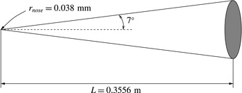
The present investigation is based on the experiments conducted by Corke et al. (Reference Corke, Cavalieri and Matlis2002) in the NASA Langley Quiet Wind Tunnel. The cone geometry considered has a semi vertex angle of
 $\unicode[STIX]{x1D703}_{c}=7^{\circ }$
, and a cone length of
 $L=0.3556~\text{m}$
(the cone length serves as the reference length scale for all simulation and graphs presented in this publication). The nose radius of this ‘sharp’ cone is
 $r_{nose}=0.038~\text{mm}$
. A schematic of this model is shown in figure 1. The approach flow of the NASA Quiet Wind Tunnel has a Mach number of 3.5 and a unit Reynolds number of
 $9.45\times 10^{6}~\text{m}^{-1}$
. The stagnation temperature and pressure are given as 310.9 K and 172 368.93 Pa, respectively. The relevant flow and computational parameters are summarized in table 1.
Cone model used for the NASA experiments. The ‘sharp’ cone has a nose radius of 0.038 mm, the semi vertex angle is
 $7^{\circ }$
and the model length is 0.3556 m.

For these conditions Laible et al. (Reference Laible, Mayer and Fasel2009) performed spatial mean-flow calculations as well as transition simulations of oblique breakdown. Laible et al. (Reference Laible, Mayer and Fasel2009) initiated the transition process by forcing a small-amplitude pair of oblique waves with frequency
 $F=4\times 10^{-5}$
(
 $\unicode[STIX]{x1D714}=151.62$
) and azimuthal wavenumber
 $k_{c}=12$
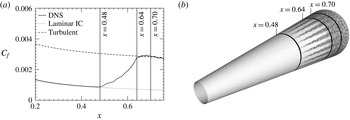
(i.e. 12 wavelengths around the circumference) close to the nose tip via wall blowing and suction. As these waves travel in the downstream direction, they experience exponential growth and generate higher harmonics and also the longitudinal vortex mode, eventually causing the boundary layer to transition. Figure 2 shows the skin friction versus downstream direction and a flow visualization of this spatial simulation. The flow visualization can be correlated to the skin friction. The highlighted positions in figure 2,
 $x=0.48$
,
 $x=0.64$
and
 $x=0.70$
indicate the onset of transition, the downstream location where the flow becomes fully turbulent and the
 $x$
-location for which the local analysis of the present temporal simulations were performed, respectively. Rather than taking the mean flow of this spatial transition simulation, the flow field for the subsequent temporal investigations was obtained by the same steady laminar mean-flow calculation, which also served as initial condition for the spatial simulation. The reason for choosing a laminar initial condition rather than a turbulent one is that the objective of the present work is to investigate the transition process from a laminar to a turbulent flow state.
Spatial simulation of oblique breakdown under the experimental conditions of Corke et al. (Reference Corke, Cavalieri and Matlis2002), (a) skin friction versus downstream direction and (b) density gradient at the constant wall-normal position
 $y=1.94\times 10^{-3}$
. The streamwise positions
 $x=0.48$
,
 $x=0.64$
and
 $x=0.7$
indicate the onset of transition, the downstream location where the flow becomes fully turbulent and the
 $x$
-location for which the temporal simulations for the present investigation were performed, respectively.

3.2 Simulation set-up
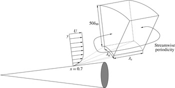
The set-up for the temporal simulations is schematically shown in figure 3. At the non-dimensional streamwise coordinate
 $x=0.7$
, the wall-normal profiles of the streamwise velocity
 $u$
, the temperature
 $T$
and the density
 $\unicode[STIX]{x1D70C}$
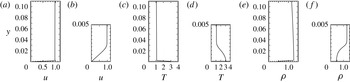
, are extracted from the steady mean-flow calculation to serve as laminar initial condition for the temporal simulations. The specific profiles are shown in figure 4. In contrast to a flat-plate boundary layer, these profiles vary outside the boundary layer, most noticeably in the density. The wall-normal velocity component,
 $v$
, is set to zero (parallel flow assumption) and the pressure,
 $p$
, is computed using the equation of state (2.2). The azimuthal velocity component,
 $w$
, of the axisymmetric initial condition is by definition equal to zero. During the entire temporal simulation, this laminar mean flow is treated by the above mentioned forcing technique and hence, the mean-flow deviation, which is only caused by the introduced disturbances, at the end of the simulation is below
 $1\times 10^{-2}$
. It is important to note that the conical coordinate system is no longer the underlying geometry for the temporal simulations. Due the body divergence, the outflow would necessarily have a larger area than the inflow, and thus, periodicity would be violated. Therefore, the geometry is changed to a cylinder with a body radius equal to the local cone radius at
 $x=0.7$
:
 $r_{0}=\sin (7^{\circ })x\approx 0.0853$
. Note that at this particular location the ratio between the boundary layer thickness and the cylinder radius is
 $\unicode[STIX]{x1D6FF}_{99}/r_{0}\approx 0.026$
. Due to this simplification in geometry some physical aspects are neglected as for example the effect of the body divergence on the growth rate of the oblique disturbances (see for example Fezer & Kloker Reference Fezer, Kloker, Zeitoun, Periaux, Desideri and Marini2003). Nevertheless, the present approach will capture the important physics in order to link the underlying physical mechanisms responsible for oblique breakdown and oblique transition.
Schematic of the temporal simulation set-up. The specific streamwise position and domain height for the subsequent simulations is
 $x=0.7$
and
 $y_{H}=50\unicode[STIX]{x1D6FF}_{99}$
, respectively.

Wall-normal profiles of streamwise velocity
 $u$
, temperature
 $T$
and density
 $\unicode[STIX]{x1D70C}$
, used as initial condition for the temporal simulations. Each of these quantities is plotted versus the entire wall-normal extent of the computational domain in (a,c) and (e). Close ups of the boundary layer are shown in (b,d) and (f).

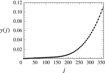
The computational domain for the temporal simulations extends in the radial direction from the cylinder wall to the free stream, which is located below the oblique shock wave originating from the cone tip. The specific wall-normal grid function used for the wall-normal direction is shown in figure 5. In the streamwise and azimuthal directions an equidistant grid-line spacing (pseudo-spectral discretization) is applied. The domain size is determined by the wavelengths of the primary disturbance wave in these directions. Therefore, as in the spatial case, the choice of the domain size in the streamwise and the azimuthal directions has a direct impact on the transition process. It appears to be logical to set the domain extent for the temporal simulation according to the wavelengths of the primary pair of oblique waves in the spatial simulation. This may, however, not result in the desired route to transition, i.e. the same route as for the spatial case, since the primary pair of oblique waves in the spatial simulation was chosen according to the global N-factor criterion, whereas for the temporal simulation, only the local temporal growth rate,
 $\unicode[STIX]{x1D714}_{i}$
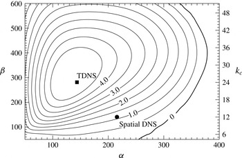
, is relevant. In order to further explain this, the temporal stability diagram, which serves as an important reference point for the set-up of transition simulations, is consulted. The stability diagram at
 $x=0.7$
shown in figure 6 was obtained by a linearized version of the temporal code. The horizontal and vertical axes in figure 6 are the streamwise wavenumber,
 $\unicode[STIX]{x1D6FC}=2\unicode[STIX]{x03C0}/\unicode[STIX]{x1D706}_{x}$
, and the azimuthal wavenumber, respectively. In particular, the left axis indicates the azimuthal wavenumber based on the surface arc length,
 $\unicode[STIX]{x1D6FD}=k_{c}/r_{0}=2\unicode[STIX]{x03C0}/\unicode[STIX]{x1D706}_{z}=2\unicode[STIX]{x03C0}/(\unicode[STIX]{x1D706}_{\unicode[STIX]{x1D711}}r_{0})$
, whereas the right axis shows the azimuthal wavenumber
 $k_{c}$
. It is important to note that although the stability diagram is continuous in the azimuthal direction only integer values of
 $k_{c}$
are possible for a cone and a cylinder.
Wall-normal grid function,
 $y(j)$
, used for the temporal investigations.

Isocontours of temporal growth rate,
 $\unicode[STIX]{x1D714}_{i}$
, in the streamwise–azimuthal wavenumber (
 $\unicode[STIX]{x1D6FC}$
–
 $\unicode[STIX]{x1D6FD}$
) plane. Two streamwise–azimuthal wavenumber combinations are marked. The solid square (▪) indicates a pair of oblique waves in the vicinity of maximum amplification, whereas the solid circle (●) indicates the pair of oblique waves whose wavelengths correspond to those of the primary disturbance wave in the spatial simulation.

Two streamwise–azimuthal wavenumber combinations are specifically marked. The solid square (▪,
 $\unicode[STIX]{x1D6FC}=143.7$
,
 $\unicode[STIX]{x1D6FD}=281.3$
) indicates a pair of oblique waves in the vicinity of maximum amplification, whereas the solid circle (●) indicates the pair of oblique waves whose wavelengths correspond to those of the primary disturbance wave in the spatial simulation at position
 $x=0.7$
, if the wave would continue with its linear eigenbehaviour (frequency:
 $F=4\times 10^{-5}$
or
 $\unicode[STIX]{x1D714}=151.62$
; streamwise wavenumber:
 $\unicode[STIX]{x1D6FC}=215.69$
and azimuthal wavenumber:
 $k_{c}=12$
or
 $\unicode[STIX]{x1D6FD}=k_{c}/r_{0}=140.68$
). The stability diagram plotted in figure 6 suggests that the primary disturbance wave from the spatial simulation (●) is located in a region of low amplification. Therefore, in order to ensure that in the following analysis the primary pair of oblique waves experiences strong exponential growth, the pair of oblique waves indicated by the black square is used to initialize oblique breakdown in the subsequent temporal simulation.
3.3 Temporal simulation
For the nonlinear transition simulation presented in the following, the primary pair of oblique waves (▪,
 $\unicode[STIX]{x1D6FC}=143.7$
,
 $\unicode[STIX]{x1D6FD}=281.3$
) is initialized using information obtained by a prior ‘linear’ simulation of this wave. If the disturbances are initially at small amplitudes, it is feasible to prescribe them as part of the initial condition by superimposing the linear disturbances,
 $$\begin{eqnarray}\unicode[STIX]{x1D719}(x,y,\unicode[STIX]{x1D711})=A_{0}a(y)\cdot \sin (\unicode[STIX]{x1D6FC}x+\unicode[STIX]{x1D703}(y))\text{trig}(k_{c}\unicode[STIX]{x1D711}),\end{eqnarray}$$
on the base flow. Note that for temporal simulations the disturbances are typically prescribed over the entire streamwise and azimuthal extent of the computational domain. As before,
 $\unicode[STIX]{x1D719}$
is the place holder for the primitive variables
 $u$
,
 $v$
,
 $w$
,
 $T$
,
 $\unicode[STIX]{x1D70C}$
and
 $p$
,
 $A_{0}$
determines the amplitude,
 $a(y)$
and
 $\unicode[STIX]{x1D703}(y)$
represent the wall-normal amplitude and phase distribution of each variable and the function
 $\text{trig}$
is equivalent to a sine for
 $w$
, whereas it represents a cosine for all other primitive variables. In particular, the amplitude of the disturbance density maximum was set to
 $|\unicode[STIX]{x1D70C}^{\prime }|_{max}=2\times 10^{-5}$
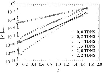
. This low value of the initial disturbance amplitude allows for an initially ‘linear’ development of the disturbances. Although this simulation does not have the necessary resolution (see table 1) for resolving the late stages of transition, and much less the turbulent regime, the linear and early nonlinear stages can be captured accurately. Figure 7 shows the evolution of the disturbance density maximum for selected modes. Note that in this paper a mode is denoted by a pair of two integers (
 $n,k$
), where
 $n=\unicode[STIX]{x1D6FC}_{n,k}/\unicode[STIX]{x1D6FC}_{1,1}$
and
 $k=\unicode[STIX]{x1D6FD}_{n,k}/\unicode[STIX]{x1D6FD}_{1,1}=k_{c,n,k}/k_{c,1,1}$
indicate the harmonics in the streamwise and azimuthal directions, respectively. Furthermore it is important to emphasize that in this context a mode is in general not the equivalent of a normal mode resulting from the eigenvalue problem of the linear stability equations. In fact, a mode in the present nomenclature can be composed of multiple normal modes, as will be explained later. Before interpreting the result plotted in figure 7, it is expedient to provide some basics regarding the nonlinear generation of higher harmonics of disturbance quantities. The inviscid Burgers equation,
 $$\begin{eqnarray}{\displaystyle \frac{\unicode[STIX]{x2202}u}{\unicode[STIX]{x2202}t}}=-{\displaystyle \frac{1}{2}}{\displaystyle \frac{\unicode[STIX]{x2202}u^{2}}{\unicode[STIX]{x2202}x}},\end{eqnarray}$$
can be considered as a simple model equation for the nonlinear terms in the Navier–Stokes equations. If we represent a mode by the wave ansatz of the following form:
 $$\begin{eqnarray}u=A_{0}\left(u_{c}(y)\cos \left(\unicode[STIX]{x1D6FC}x-\unicode[STIX]{x1D714}t\right)+u_{s}(y)\sin \left(\unicode[STIX]{x1D6FC}x-\unicode[STIX]{x1D714}t\right)\right)\cos \left(\unicode[STIX]{x1D6FD}z\right)\text{e}^{\unicode[STIX]{x1D70E}t},\end{eqnarray}$$
then the nonlinear term
 $u^{2}$
can be calculated as,
 $$\begin{eqnarray}\displaystyle u^{2} & = & \displaystyle {\displaystyle \frac{A_{0}^{2}\text{e}^{2\unicode[STIX]{x1D70E}t}}{4}}\left(\left(u_{c}^{2}+u_{s}^{2}\right)\right.+\left(u_{c}^{2}-u_{s}^{2}\right)\cos \left(2\unicode[STIX]{x1D6FC}x-2\unicode[STIX]{x1D714}t\right)\nonumber\\ \displaystyle & & \displaystyle \left.+\;2u_{c}u_{s}\sin \left(2\unicode[STIX]{x1D6FC}x-2\unicode[STIX]{x1D714}t\right)\right)\left(1+\cos \left(2\unicode[STIX]{x1D6FD}z\right)\right).\end{eqnarray}$$
In the above equations,
 $\unicode[STIX]{x1D6FC}$
and
 $\unicode[STIX]{x1D6FD}$
denote the streamwise and spanwise wavenumbers, respectively,
 $\unicode[STIX]{x1D714}$
is the angular frequency,
 $A_{0}$
is the amplitude,
 $u_{c}(y)$
and
 $u_{s}(y)$
with
 $\sqrt{u_{c}^{2}+u_{s}^{2}}|_{max}=1$
are the wall-normal velocity distributions corresponding to the cosine and sine part of the wave, respectively and
 $\unicode[STIX]{x1D70E}$
is the temporal growth rate. In order to have a clear distinction from the angular frequency,
 $\unicode[STIX]{x1D714}$
, and also to avoid unnecessary subscripts,
 $\unicode[STIX]{x1D70E}$
instead of
 $\unicode[STIX]{x1D714}_{i}$
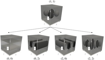
was chosen to denote the temporal growth rate in the above as well as subsequent equations. Two aspects can be inferred from (3.4): (i) the nonlinear term is proportional to the square of the amplitude of the primary mode and, hence, has twice the growth rate of the primary mode and (ii) the modes that are nonlinearly generated by the interaction of mode (
 $1,1$
) with itself are the modes (
 $0,0$
), (
 $0,2$
), (
 $2,0$
) and (
 $2,2$
). In this work, these modes are referred to as the first level of nonlinearly generated modes and are schematically shown in figure 9. A mode of the second level of nonlinearly generated modes is, for example, mode (
 $1,3$
), which is generated by the interaction between the modes (
 $1,1$
) and (
 $0,2$
) as well as by the interaction between modes (
 $1,1$
) and (
 $2,2$
). Modes of the second level grow with a rate which is three times faster than that of the primary wave. Clearly, employing the Burgers equation as a model is not providing the entire story, because differentiating
 $u^{2}$
with respect to
 $x$
eliminates the modes (
 $0,0$
) and (
 $0,2$
). However, one can see that this is not true for the complete Navier–Stokes equations that have additional nonlinear terms, i.e. terms which are differentiated with respect to
 $y$
and
 $\unicode[STIX]{x1D711}/z$
, as will be shown later.
Temporal development of the disturbance density maximum of selected modes
 $(n,k)$
.

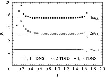
Temporal development of the growth rate of the disturbance density maximum of selected modes.

Schematic of modes generated directly by the primary pair of oblique waves (first level of nonlinearly generated modes).

Returning to the interpretation of figure 7, it can be observed that the first level of nonlinearly generated modes as well as mode (
 $1,3$
) from the second level develop in this temporal simulation (due to the presence of mode (
 $1,1$
)). This is in qualitative agreement with the spatial simulations. Furthermore, the flow field exhibits the signature features of oblique breakdown, e.g. mode (
 $0,2$
) is throughout the simulation at a significant higher amplitude level than the other modes of the first level of nonlinearly generated modes. Further insight can be gained by considering the growth rates of the most important modes of oblique breakdown, namely modes (
 $0,2$
) and (
 $1,3$
), which are plotted in figure 8. As stated earlier, if the emergence of mode (
 $0,2$
) and mode (
 $1,3$
) is a result of nonlinear interactions, then their growth rates should be twice and three times the growth rate of the primary pair of oblique waves (mode
 $1,1$
), respectively. This is indeed the case, therefore this simulation exhibits all features of the early nonlinear regime of oblique breakdown and hence will be analysed in detail in the next section.
4 Analysis
The key feature of oblique breakdown in the nonlinear regime is the strong growth of the steady mode (
 $0,2$
) early in the transition process. The emergence of this mode has been recognized by Fasel et al. (Reference Fasel, Thumm, Bestek, Kral and Zang1993) to be a direct consequence of the nonlinear interaction between the two primary oblique waves with the same, but opposite, wave angles, namely mode (
 $1,1$
). However, as noted above, not only mode (
 $0,2$
) is generated by the primary pair of oblique waves but also modes (
 $0,0$
), (
 $2,0$
) and (
 $2,2$
). Although these additional modes are, like mode (
 $0,2$
), a direct consequence of the primary pair of oblique waves and have the same growth rate as mode (
 $0,2$
), their amplitudes are typically significantly lower than the amplitude of mode (
 $0,2$
), as shown for the simulation plotted in figure 7. In particular, after the initial transient at
 $t\approx 0.4$
, modes (
 $0,0$
), (
 $2,0$
) and (
 $2,2$
) are at the same amplitude level, which is, by a factor of
 $19.45$
, lower than the amplitude of mode (
 $0,2$
).
In order to achieve the goal of completely understanding the different amplitude levels of the nonlinearly generated modes in oblique breakdown, first the ‘energy’ transferred from mode (
 $1,1$
) to the modes (
 $0,0$
), (
 $0,2$
), (
 $2,0$
) and (
 $2,2$
) is analysed in more detail. The reason we put the term ‘energy’ in quotes is that rather than looking at energy, for simplicity we are considering the evolution of the disturbance density, which is governed by the continuity equation,
 $$\begin{eqnarray}{\displaystyle \frac{\unicode[STIX]{x2202}\unicode[STIX]{x1D70C}}{\unicode[STIX]{x2202}t}}+{\displaystyle \frac{\unicode[STIX]{x2202}\unicode[STIX]{x1D70C}u}{\unicode[STIX]{x2202}x}}+{\displaystyle \frac{\unicode[STIX]{x2202}\unicode[STIX]{x1D70C}v}{\unicode[STIX]{x2202}y}}+{\displaystyle \frac{1}{r}}{\displaystyle \frac{\unicode[STIX]{x2202}\unicode[STIX]{x1D70C}w}{\unicode[STIX]{x2202}\unicode[STIX]{x1D711}}}+{\displaystyle \frac{\unicode[STIX]{x1D70C}v}{r}}=0.\end{eqnarray}$$
If only the primary pair of oblique waves, mode (
 $1,1$
), is considered the evolution of the density will be governed by,
 $$\begin{eqnarray}{\displaystyle \frac{\unicode[STIX]{x2202}\unicode[STIX]{x1D70C}_{nl}^{\prime }}{\unicode[STIX]{x2202}t}}=-\left({\displaystyle \frac{\unicode[STIX]{x2202}\unicode[STIX]{x1D70C}_{1,1}u_{1,1}}{\unicode[STIX]{x2202}x}}+{\displaystyle \frac{\unicode[STIX]{x2202}\unicode[STIX]{x1D70C}_{1,1}v_{1,1}}{\unicode[STIX]{x2202}y}}+{\displaystyle \frac{1}{r}}{\displaystyle \frac{\unicode[STIX]{x2202}\unicode[STIX]{x1D70C}_{1,1}w_{1,1}}{\unicode[STIX]{x2202}\unicode[STIX]{x1D711}}}+{\displaystyle \frac{\unicode[STIX]{x1D70C}_{1,1}v_{1,1}}{r}}\right),\end{eqnarray}$$
where the subscript
 $_{nl}$
indicates generation via nonlinear mechanisms. Note that in this and the following formulae, the disturbances created by mode (
 $1,1$
) are indicated by a prime, whereas no prime is used for mode (
 $1,1$
) itself. The primitive variables of mode (
 $1,1$
) are known a priori. They can be obtained from a small-amplitude (linear) temporal simulation (as was done in the present case) or a linear stability theory (LST) analysis, for example. The individual wave components are represented using the wave ansatz as,
 $$\begin{eqnarray}\unicode[STIX]{x1D719}=A_{0}\left(\unicode[STIX]{x1D719}_{c}(y)\cos (\unicode[STIX]{x1D6FC}x-\unicode[STIX]{x1D714}t)+\unicode[STIX]{x1D719}_{s}(y)\sin (\unicode[STIX]{x1D6FC}x-\unicode[STIX]{x1D714}t)\right)\text{trig}(k_{c}\unicode[STIX]{x1D711})\text{e}^{\unicode[STIX]{x1D70E}t},\end{eqnarray}$$
where
 $\unicode[STIX]{x1D719}$
is a placeholder for the flow variables
 $u$
,
 $v$
,
 $w$
and
 $\unicode[STIX]{x1D70C}$
, for which the subscript
 $1,1$
is dropped for convenience.
 $A_{0}$
is the wave amplitude at time
 $t=0$
,
 $\unicode[STIX]{x1D719}_{c}(y)$
and
 $\unicode[STIX]{x1D719}_{s}(y)$
are the Fourier coefficients for the cosine and sine part, respectively (note that
 $\sqrt{\unicode[STIX]{x1D70C}_{c}^{2}+\unicode[STIX]{x1D70C}_{s}^{2}}|_{max}=1$
),
 $\unicode[STIX]{x1D6FC}$
,
 $k_{c}=\unicode[STIX]{x1D6FD}r_{0}$
and
 $\unicode[STIX]{x1D714}$
denote the streamwise wavenumber, the azimuthal wavenumber and the frequency, respectively, and
 $\unicode[STIX]{x1D70E}=\unicode[STIX]{x1D714}_{i}$
is the temporal growth rate. The function
 $\text{trig}$
has the same definition as in (3.1). The individual terms of the continuity equation are calculated by first multiplying the density with the different velocity components and afterwards applying the derivatives with respect to either
 $x$
,
 $y$
and
 $\unicode[STIX]{x1D711}$
to the different terms. By inserting these terms into (4.2) the resulting equation for the temporal derivative of the density can be written as
 $$\begin{eqnarray}\displaystyle {\displaystyle \frac{\unicode[STIX]{x2202}\unicode[STIX]{x1D70C}_{nl}^{\prime }}{\unicode[STIX]{x2202}t}}=-{\displaystyle \frac{A_{0}^{2}\text{e}^{2\unicode[STIX]{x1D70E}t}}{4}}\tilde{\unicode[STIX]{x1D70C}_{nl}}(y), & & \displaystyle\end{eqnarray}$$
with
 $$\begin{eqnarray}\displaystyle \tilde{\unicode[STIX]{x1D70C}_{nl}}(y) & = & \displaystyle (\!\hat{\unicode[STIX]{x1D70C}}_{0,0,nl}(y)+\hat{\unicode[STIX]{x1D70C}}_{0,2,nl}(y)\cos (2k_{c}\unicode[STIX]{x1D711})\nonumber\\ \displaystyle & & \displaystyle +\,\hat{\unicode[STIX]{x1D70C}}_{2,0,c,nl}(y)\cos (2\unicode[STIX]{x1D6FC}x-2\unicode[STIX]{x1D714}t)+\hat{\unicode[STIX]{x1D70C}}_{2,0,s,nl}(y)\sin (2\unicode[STIX]{x1D6FC}x-2\unicode[STIX]{x1D714}t)\nonumber\\ \displaystyle & & \displaystyle +(\!\hat{\unicode[STIX]{x1D70C}}_{2,2,c,nl}(y)\cos (2\unicode[STIX]{x1D6FC}x-2\unicode[STIX]{x1D714}t)\nonumber\\ \displaystyle & & \displaystyle +\,\hat{\unicode[STIX]{x1D70C}}_{2,2,s,nl}(y)\sin (2\unicode[STIX]{x1D6FC}x-2\unicode[STIX]{x1D714}t))\cos (2k_{c}\unicode[STIX]{x1D711})\!),\end{eqnarray}$$
where the individual terms are given as,
 $$\begin{eqnarray}\displaystyle \hat{\unicode[STIX]{x1D70C}}_{0,0,nl}(y) & = & \displaystyle \left(\unicode[STIX]{x1D70C}_{c}|_{y}v_{c}+\unicode[STIX]{x1D70C}_{c}v_{c}|_{y}+\unicode[STIX]{x1D70C}_{s}|_{y}v_{s}+\unicode[STIX]{x1D70C}_{s}v_{s}|_{y}+{\displaystyle \frac{1}{r}}(\unicode[STIX]{x1D70C}_{c}v_{c}+\unicode[STIX]{x1D70C}_{s}v_{s})\right),\end{eqnarray}$$
 $$\begin{eqnarray}\displaystyle \hat{\unicode[STIX]{x1D70C}}_{0,2,nl}(y) & = & \displaystyle \left(\unicode[STIX]{x1D70C}_{c}|_{y}v_{c}+\unicode[STIX]{x1D70C}_{c}v_{c}|_{y}+\unicode[STIX]{x1D70C}_{s}|_{y}v_{s}+\unicode[STIX]{x1D70C}_{s}v_{s}|_{y}+{\displaystyle \frac{1}{r}}(\unicode[STIX]{x1D70C}_{c}v_{c}+\unicode[STIX]{x1D70C}_{s}v_{s})\right.\nonumber\\ \displaystyle & & \displaystyle \left.+\,2{\displaystyle \frac{k_{c}}{r}}(\unicode[STIX]{x1D70C}_{c}w_{c}+\unicode[STIX]{x1D70C}_{s}w_{s})\right),\end{eqnarray}$$
 $$\begin{eqnarray}\displaystyle \hat{\unicode[STIX]{x1D70C}}_{2,0,c,nl}(y) & = & \displaystyle \left(\vphantom{\frac{1}{2}}(\unicode[STIX]{x1D70C}_{c}u_{s}+\unicode[STIX]{x1D70C}_{s}u_{c})2\unicode[STIX]{x1D6FC}+(\unicode[STIX]{x1D70C}_{c}|_{y}v_{c}+\unicode[STIX]{x1D70C}_{c}v_{c}|_{y}-\unicode[STIX]{x1D70C}_{s}|_{y}v_{s}-\unicode[STIX]{x1D70C}_{s}v_{s}|_{y})\right.\nonumber\\ \displaystyle & & \displaystyle \left.+\,{\displaystyle \frac{1}{r}}(\unicode[STIX]{x1D70C}_{c}v_{c}-\unicode[STIX]{x1D70C}_{s}v_{s})\right),\end{eqnarray}$$
 $$\begin{eqnarray}\displaystyle \hat{\unicode[STIX]{x1D70C}}_{2,0,s,nl}(y) & = & \displaystyle \left(\vphantom{\frac{1}{2}}(-\unicode[STIX]{x1D70C}_{c}u_{c}+\unicode[STIX]{x1D70C}_{s}u_{s})2\unicode[STIX]{x1D6FC}+(\unicode[STIX]{x1D70C}_{c}|_{y}v_{s}+\unicode[STIX]{x1D70C}_{c}v_{s}|_{y}+\unicode[STIX]{x1D70C}_{s}|_{y}v_{c}+\unicode[STIX]{x1D70C}_{s}v_{c}|_{y})\right.\nonumber\\ \displaystyle & & \displaystyle \left.+\,{\displaystyle \frac{1}{r}}(\unicode[STIX]{x1D70C}_{c}v_{s}+\unicode[STIX]{x1D70C}_{s}v_{c})\right),\end{eqnarray}$$
 $$\begin{eqnarray}\displaystyle \hat{\unicode[STIX]{x1D70C}}_{2,2,c,nl}(y) & = & \displaystyle \left(\vphantom{\frac{1}{2}}(\unicode[STIX]{x1D70C}_{c}u_{s}+\unicode[STIX]{x1D70C}_{s}u_{c})2\unicode[STIX]{x1D6FC}+(\unicode[STIX]{x1D70C}_{c}|_{y}v_{c}+\unicode[STIX]{x1D70C}_{c}v_{c}|_{y}-\unicode[STIX]{x1D70C}_{s}|_{y}v_{s}-\unicode[STIX]{x1D70C}_{s}v_{s}|_{y})\right.\nonumber\\ \displaystyle & & \displaystyle \left.+\,{\displaystyle \frac{1}{r}}(\unicode[STIX]{x1D70C}_{c}v_{c}-\unicode[STIX]{x1D70C}_{s}v_{s})+2{\displaystyle \frac{k_{c}}{r}}(\unicode[STIX]{x1D70C}_{c}w_{c}-\unicode[STIX]{x1D70C}_{s}w_{s})\right),\end{eqnarray}$$
 $$\begin{eqnarray}\displaystyle \hat{\unicode[STIX]{x1D70C}}_{2,2,s,nl}(y) & = & \displaystyle \left(\vphantom{\frac{1}{2}}(-\unicode[STIX]{x1D70C}_{c}u_{s}+\unicode[STIX]{x1D70C}_{s}u_{c})2\unicode[STIX]{x1D6FC}+(\unicode[STIX]{x1D70C}_{c}|_{y}v_{s}+\unicode[STIX]{x1D70C}_{c}v_{s}|_{y}+\unicode[STIX]{x1D70C}_{s}|_{y}v_{c}+\unicode[STIX]{x1D70C}_{s}v_{c}|_{y})\right.\nonumber\\ \displaystyle & & \displaystyle \left.+\,{\displaystyle \frac{1}{r}}(\unicode[STIX]{x1D70C}_{c}v_{s}+\unicode[STIX]{x1D70C}_{s}v_{c})+2{\displaystyle \frac{k_{c}}{r}}(\unicode[STIX]{x1D70C}_{c}w_{s}+\unicode[STIX]{x1D70C}_{s}w_{c})\right).\end{eqnarray}$$
 $0,0$
), (
 $0,2$
), (
 $2,0$
) and (
 $2,2$
), appear in this equation and are hence a direct result of the nonlinear interaction of mode (
 $1,1$
) with itself. In order to validate this stage of the theoretical considerations, the result of (4.4)–(4.6a
–
f
) is compared with the right-hand side of the continuity equation (which is
 $\unicode[STIX]{x2202}\unicode[STIX]{x1D70C}^{\prime }/\unicode[STIX]{x2202}t$
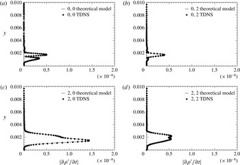
), calculated by the temporal Navier–Stokes solver in figure 10.
Comparison of the wall-normal amplitude distribution of
 $\unicode[STIX]{x2202}\unicode[STIX]{x1D70C}^{\prime }/\unicode[STIX]{x2202}t$
obtained by (4.4) and the wall-normal amplitude distribution of
 $\unicode[STIX]{x2202}\unicode[STIX]{x1D70C}^{\prime }/\unicode[STIX]{x2202}t$
obtained by the Navier–Stokes solver for the nonlinearly generated modes (
 $0,0$
), (
 $0,2$
), (
 $2,0$
) and (
 $2,2$
) (a–d).

The flow field from which the Navier–Stokes solver calculates
 $\unicode[STIX]{x2202}\unicode[STIX]{x1D70C}^{\prime }/\unicode[STIX]{x2202}t$
is initialized with the mean flow (see figure 4) and the primary pair of oblique waves with the maximum density amplitude of
 $|\unicode[STIX]{x1D70C}^{\prime }|_{max}=2\times 10^{-5}$
. The agreement for all four nonlinearly generated modes is excellent, thus suggesting that up to this point the theoretical considerations are correct.
By integrating equation (4.4) in time an expression for the evolution of the density that is purely based on the nonlinear generation due to mode (
 $1,1$
) is obtained. For the steady modes (mode
 $0,0$
and mode
 $0,2$
) the integration is straightforward and results in
 $$\begin{eqnarray}\unicode[STIX]{x1D70C}_{nl}^{\prime }(t)=\unicode[STIX]{x1D70C}^{\prime }(t=0)-{\displaystyle \frac{A_{0}^{2}}{4}}\tilde{\unicode[STIX]{x1D70C}}_{steady,nl}(y){\displaystyle \frac{1}{2\unicode[STIX]{x1D70E}}}(\text{e}^{2\unicode[STIX]{x1D70E}t}-1).\end{eqnarray}$$
By setting the initial amplitude of each mode to zero (
 $\unicode[STIX]{x1D70C}^{\prime }(t=0)=0$
), the temporal development of the maximum disturbance amplitude of the two steady modes can then be calculated according to
 $$\begin{eqnarray}\unicode[STIX]{x1D70C}_{0,k,nl,max}^{\prime }={\displaystyle \frac{A_{0}^{2}}{4}}|\hat{\unicode[STIX]{x1D70C}}_{0,k,nl}(y)|_{max}{\displaystyle \frac{1}{2\unicode[STIX]{x1D70E}}}(\text{e}^{2\unicode[STIX]{x1D70E}t}-1),\end{eqnarray}$$
where the subscript
 $max$
indicates the maximum in wall-normal direction and the index
 $k$
represents the azimuthal mode that is either
 $k=0$
or
 $k=2$
. For the unsteady modes, that is mode (
 $2,0$
) and mode (
 $2,2$
), the integration has to consider the phase velocity that is assumed for the particular mode. A constant phase speed can be modelled by adding the convection term
 $-c\cdot \unicode[STIX]{x2202}\unicode[STIX]{x1D70C}/\unicode[STIX]{x2202}x$
to the right-hand side of (4.4). The resulting equation has then the form of a forced wave equation,
 $$\begin{eqnarray}{\displaystyle \frac{\unicode[STIX]{x2202}\unicode[STIX]{x1D70C}_{nl}^{\prime }}{\unicode[STIX]{x2202}t}}=-c{\displaystyle \frac{\unicode[STIX]{x2202}\unicode[STIX]{x1D70C}_{nl}^{\prime }}{\unicode[STIX]{x2202}x}}-{\displaystyle \frac{A_{0}^{2}\text{e}^{2\unicode[STIX]{x1D70E}t}}{4}}\tilde{\unicode[STIX]{x1D70C}_{nl}}(y).\end{eqnarray}$$
If it is further assumed that
 $\unicode[STIX]{x1D70C}_{nl}^{\prime }$
can be expressed by the wave ansatz (using the example of mode
 $2,0$
),
 $$\begin{eqnarray}\unicode[STIX]{x1D70C}_{2,0,nl}^{\prime }=\unicode[STIX]{x1D70C}_{2,0,c,nl}^{\prime }(y,t)\cos (2\unicode[STIX]{x1D6FC}x-2\unicode[STIX]{x1D714}t)+\unicode[STIX]{x1D70C}_{2,0,s,nl}^{\prime }(y,t)\sin (2\unicode[STIX]{x1D6FC}x-2\unicode[STIX]{x1D714}t).\end{eqnarray}$$
Then the resulting expression will be a coupled equation, which can be conveniently written in matrix form,
 $$\begin{eqnarray}{\displaystyle \frac{\unicode[STIX]{x2202}}{\unicode[STIX]{x2202}t}}\left(\begin{array}{@{}c@{}}\unicode[STIX]{x1D70C}_{2,0,c,nl}^{\prime }\\ \unicode[STIX]{x1D70C}_{2,0,s,nl}^{\prime }\end{array}\right)=2\left(\unicode[STIX]{x1D714}-c\unicode[STIX]{x1D6FC}\right)\left(\begin{array}{@{}cc@{}}0 & 1\\ -1 & 0\end{array}\right)\left(\begin{array}{@{}c@{}}\unicode[STIX]{x1D70C}_{2,0,c,nl}^{\prime }\\ \unicode[STIX]{x1D70C}_{2,0,s,nl}^{\prime }\end{array}\right)-{\displaystyle \frac{A_{0}^{2}\text{e}^{2\unicode[STIX]{x1D70E}t}}{4}}\left(\begin{array}{@{}c@{}}\hat{\unicode[STIX]{x1D70C}}_{2,0,c,nl}\\ \hat{\unicode[STIX]{x1D70C}}_{2,0,s,nl}\end{array}\right).\end{eqnarray}$$
If the phase velocity of mode (
 $2,0$
) is set to the phase velocity of the primary wave, i.e.
 $c=\unicode[STIX]{x1D714}/\unicode[STIX]{x1D6FC}$
, then the system is decoupled and can be easily integrated. By performing the same integration as for the steady modes, the evolution of the density maximum for mode (
 $2,0$
) and equivalently for mode (
 $2,2$
) can be predicted by
 $$\begin{eqnarray}\unicode[STIX]{x1D70C}_{2,k,max,nl}^{\prime }={\displaystyle \frac{A_{0}^{2}}{4}}\sqrt{\hat{\unicode[STIX]{x1D70C}}_{2,k,c,nl}(y)^{2}+\hat{\unicode[STIX]{x1D70C}}_{2,k,s,nl}(y)^{2}}|_{max}{\displaystyle \frac{1}{2\unicode[STIX]{x1D70E}}}(\text{e}^{2\unicode[STIX]{x1D70E}t}-1),\end{eqnarray}$$
where the subscript
 $max$
indicates the maximum in wall-normal direction and the index
 $k$
represents the azimuthal mode that is either
 $k=0$
or
 $k=2$
. It is apparent that all four nonlinearly generated modes have the same growth rate, namely
 $2\unicode[STIX]{x1D70E}t$
if
 $t\rightarrow \infty$
. Due to the forcing terms, however, the amplitudes may be different.
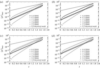
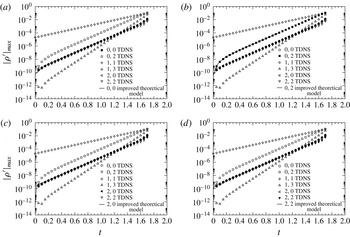
Comparison of the development of the disturbance density maximum for each nonlinearly generated mode, (
 $0,0$
), (
 $0,2$
), (
 $2,0$
) and (
 $2,2$
) (a–d), between the TDNS and the theoretical model. Note that in each graph the TDNS mode that is compared to the theoretical model is plotted with solid symbols.

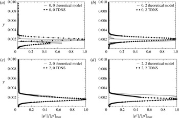
Therefore, it is now left to check how well this model approximates the early nonlinear stages simulated by the temporal direct numerical simulation (TDNS) and if it can explain the difference in amplitude between the nonlinearly generated modes. A comparison between the results obtained from the TDNS, and the theoretical model is provided in figure 11, where the amplitude evolution of each mode is plotted versus time. In each of the four graphs a different mode of the TDNS is highlighted and compared to the theoretical model. In general, although the growth rates of the nonlinearly generated modes agree, there are discrepancies in the amplitudes between the TDNS and the theoretical model. Among all four modes the best agreement is achieved for mode (
 $0,0$
), whereas the largest deviation is apparent for the amplitude of mode (
 $0,2$
), which is estimated at a significantly lower amplitude level. It is interesting to note that the model predicts the amplitude of mode (
 $0,2$
) at the same level as the other nonlinearly generated modes for the entire time interval. This suggests that the nonlinear forcing does not fully explain the development of mode (
 $0,2$
) or the development of the other modes. This conjecture is further supported by figure 12, in which the normalized wall-normal amplitude distributions extracted at time
 $t=1.0$
are plotted for each mode. Except for mode (
 $2,0$
) there is poor agreement between the TDNS and the theoretical nonlinear model. In particular, the wall-normal maximum of the steady modes (modes
 $0,0$
and
 $0,2$
) is predicted farther outward than simulated by the TDNS. Moreover, the shape of mode (
 $2,2$
) does not agree at all with the one extracted from the TDNS. In conclusion, there has to be another mechanism that strongly influences the amplitude level of the nonlinearly generated modes, and especially the amplitude of mode (
 $0,2$
) – the signature mode of oblique breakdown. Additional forcing due to nonlinear interaction of other modes can be ruled out since there are no further modes at an amplitude level that is sufficiently high to cause an amplitude rise in mode (
 $0,2$
) to the observed level. Furthermore, the growth rate being twice the growth rate of the primary wave suggests that this is the dominant source of nonlinear forcing.
Comparison of the normalized wall-normal amplitude distribution of the disturbance density for each nonlinearly generated mode, (
 $0,0$
), (
 $0,2$
), (
 $2,0$
) and (
 $2,2$
) (a–d), between the TDNS and the theoretical model.

Therefore, it is conjectured that the linear eigenbehaviour may be essential in raising the amplitude level of mode (
 $0,2$
). In order to identify if that is indeed the case, the following steps are subsequently performed: (i) a TDNS is performed for a single Runge–Kutta time step,
 $\unicode[STIX]{x0394}t=1\times 10^{-5}$
; (ii) the amplitude and phase distributions for each of the four nonlinearly generated modes are extracted after this one time step and compared to the theoretical model (if the agreement is good, it can be concluded that for a short time period,
 $t\ll 1$
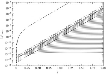
, the theoretical model captures the essential physics); (iii) for each mode one ‘linear’ simulation is conducted, where the initial condition is composed of the mean flow and the particular mode extracted from the TDNS after one time step; (iv) by combining the theoretical model for the nonlinear forcing with the linear eigenbehaviour the amplitude for each mode can be calculated by superposition; and (v) if the agreement with the results obtained from TDNS is good, it can be concluded that both nonlinear forcing and eigenbehaviour are relevant for the amplitude of the nonlinearly generated modes.
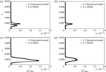
Comparison of the wall-normal amplitude distribution of the disturbance density for each nonlinearly generated mode, (
 $0,0$
), (
 $0,2$
), (
 $2,0$
) and (
 $2,2$
) (a–d), between the TDNS and the theoretical model after one Runge–Kutta time step,
 $\unicode[STIX]{x0394}t=1\times 10^{-5}$
.

Steps (i) and (ii) are easily performed and the resulting wall-normal amplitude distribution of the disturbance density for each mode is shown in figure 13. The comparison between the theoretical model and the TDNS is good, although minor differences are apparent for the modes (
 $0,0$
), (
 $0,2$
) and (
 $2,2$
). Therefore, it can be concluded that after one time step the resulting wall-normal amplitude and phase distribution of the nonlinearly generated modes, (
 $0,0$
), (
 $0,2$
), (
 $2,0$
) and (
 $2,2$
), are purely due to the nonlinear forcing of mode (
 $1,1$
). Hence the theoretical model captures the relevant physics for small times,
 $t\ll 1$
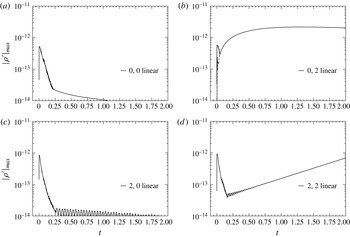
. In step (iii) the linear (or eigen) response to the wall-normal amplitude distributions that are due to (and only due to) the nonlinear forcing are used as initial condition for four subsequent simulations, in which the linear behaviour of each of the four nonlinearly generated modes is simulated. The resulting amplitude development for each mode is plotted in figure 14. All four nonlinearly generated modes exhibit the common feature that the linear development of the disturbances forced into each particular mode experiences a strong increase in amplitude followed by strong decay. Using mode (
 $0,2$
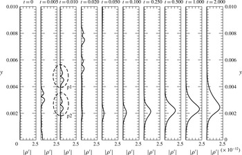
) as an example, the results displayed in figure 15 imply that the amplitude peak can be attributed to acoustic waves. These waves develop because the nonlinear generated disturbances that are seeded into mode (
 $0,2$
) do not only contain boundary layer modes but have also contributions from the entire spectrum, i.e. also from the acoustic waves. After being generated, these acoustic waves (the acoustic wave packet p1 highlighted at
 $t=0.010$
) travel in the radial direction away from the wall and eventually leave the computational domain through the free-stream boundary. Note that there is a second acoustic wave packet (p2 highlighted at
 $t=0.010$
), which initially travels towards the wall. The distance this wave packet can travel in the direction of the wall is, however, rather short (of the order of the boundary layer thickness) and once it reaches the wall (at
 $t=0.005$
) it is reflected and also travels toward the free stream. The decay experienced by these two packets is at least in parts due to the grid stretching, that is the wall-normal grid is getting coarser with distance from the wall. For the following analysis, the development of large acoustic waves is acknowledged, but because the main interest is in the boundary layer, the amplitude peak in each mode is disregarded for the time being and the focus is turned to examining the amplitude development in the boundary layer, i.e. after the decay of these peaks.
Linear evolution of the disturbance density maximum versus time of the nonlinearly generated modes (
 $0,0$
), (
 $0,2$
), (
 $2,0$
) and (
 $2,2$
) (a–d). Note that for mode (
 $0,2$
), in addition to the disturbance density maximum, the disturbance maximum in the interval
 $0<y<0.004$
is also plotted (
 $--$
).

Linear evolution of the wall-normal disturbance density profiles for the nonlinearly generated mode (
 $0,2$
). At time
 $t=0.010$
the acoustic wave packets p1 and p2, which travel in radial direction away from the wall, are highlighted by dashed ellipses. Note that the time intervals between subsequent profiles are not identical.

Figure 14 shows that mode (
 $0,0$
), as expected, decays with time. Mode (
 $2,0$
) also shows initially a strong decay followed by a more gradual decay, which exhibits oscillations in the amplitude. These oscillations, which may be attributed to the superposition of multiple decaying normal modes, are, however, not of primary importance to the present analysis. The important fact is that mode (
 $2,0$
) decays. Mode (
 $2,2$
) initially also decays, but eventually grows exponentially. Referring to the stability diagram (figure 6) where mode (
 $2,2$
) corresponds to a wave with the streamwise wavenumber
 $\unicode[STIX]{x1D6FC}=287.42$
and the azimuthal wavenumber based on the surface arc length
 $\unicode[STIX]{x1D6FD}=562.66$
, this result does not come as a surprise since mode (
 $2,2$
) is located in the unstable region.
In contrast to the modes (
 $0,0$
), (
 $2,0$
) and (
 $2,2$
), mode (
 $0,2$
) does not decay initially. Instead it shows a strong rise in amplitude and is also the only mode that surpasses, in the simulated time interval, the amplitude of the acoustic wave packet (see figure 15). In order to highlight the steep rise in amplitude, the disturbance density maximum disregarding the acoustic wave components (dashed line) is plotted in figure 14, in addition to the linear evolution of mode (
 $0,2$
) based on the disturbance density maximum. After the steep rise in amplitude, mode (
 $0,2$
) remains for a significant time at a high amplitude level before it starts to gradually decay at
 $t\approx 1.25$
. Since the growth of mode (
 $0,2$
) is by no means exponential, it must be due to non-modal or transient growth. Therefore the conjecture of Schmid & Henningson (Reference Schmid and Henningson1992) is supported by the present findings. Moreover, it is interesting to note that the wall-normal position of the disturbance density maximum moves away from the wall as time increases (see figure 15). This explains the difference in the position of the wall-normal maximum between (4.8) and the TDNS as shown in figure 12.
Using the linear behaviour of an individual disturbance, the theoretical model can be significantly improved. Because the amplitude evolution of each individual disturbance is linear, this can be done by linear superposition.
The corresponding formulae are for the steady modes:
 $$\begin{eqnarray}\unicode[STIX]{x1D70C}_{0,k}^{\prime }(t)=\int _{0}^{t}{\displaystyle \frac{\unicode[STIX]{x2202}\unicode[STIX]{x1D70C}_{0,k,nl}^{\prime }}{\unicode[STIX]{x2202}\tilde{t}}}(\tilde{t})\unicode[STIX]{x1D70C}_{0,k,lin}^{\prime }(t-\tilde{t})\,\text{d}\tilde{t},\end{eqnarray}$$
and for the unsteady modes,
 $$\begin{eqnarray}\unicode[STIX]{x1D70C}_{2,k,c}^{\prime }(t)=\int _{0}^{t}{\displaystyle \frac{\unicode[STIX]{x2202}\unicode[STIX]{x1D70C}_{2,k,nl}^{\prime }}{\unicode[STIX]{x2202}\tilde{t}}}(\tilde{t})\unicode[STIX]{x1D70C}_{2,k,lin}^{\prime }(t-\tilde{t})\cos (\unicode[STIX]{x1D719}_{2,k,lin}(t-\tilde{t})-2\unicode[STIX]{x1D714}\tilde{t})\,\text{d}\tilde{t},\end{eqnarray}$$
 $$\begin{eqnarray}\unicode[STIX]{x1D70C}_{2,k,s}^{\prime }(t)=\int _{0}^{t}{\displaystyle \frac{\unicode[STIX]{x2202}\unicode[STIX]{x1D70C}_{2,k,nl}^{\prime }}{\unicode[STIX]{x2202}\tilde{t}}}(\tilde{t})\unicode[STIX]{x1D70C}_{2,k,lin}^{\prime }(t-\tilde{t})\sin (\unicode[STIX]{x1D719}_{2,k,lin}(t-\tilde{t})-2\unicode[STIX]{x1D714}\tilde{t})\,\text{d}\tilde{t},\end{eqnarray}$$
 $\unicode[STIX]{x1D719}_{n,k,lin}(t)$
and
 $$\begin{eqnarray}\unicode[STIX]{x1D70C}_{n,k,lin}^{\prime }(t)={\displaystyle \frac{\unicode[STIX]{x1D70C}_{n,k,lin,simu}^{\prime }(\unicode[STIX]{x0394}t,t)}{\unicode[STIX]{x1D70C}_{n,k,nl}^{\prime }(\unicode[STIX]{x0394}t)}}\end{eqnarray}$$
represent the linear wall-normal phase and wall-normal amplitude evolution of each mode.
The wall-normal amplitude evolution obtained by the simulation,
 $\unicode[STIX]{x1D70C}_{n,k,lin,simu}^{\prime }(\unicode[STIX]{x0394}t,t)$
, with a certain time step
 $\unicode[STIX]{x0394}t$
has been normalized by the initial amplitude of the nonlinearly generated disturbances in order to eliminate the dependency on the numerical time step. Note that due to the phase velocity of the primary pair of oblique waves, mode (
 $1,1$
), the formulae for the unsteady modes have to account for the phase shift,
 $-2\unicode[STIX]{x1D714}t$
, between the subsequently imposed disturbances. Since (4.13) and (4.14b
) cannot be evaluated analytically, because the functions
 $\unicode[STIX]{x1D719}_{2,k,lin}(t)$
and
 $\unicode[STIX]{x1D70C}_{n,k,lin,simu}^{\prime }(\unicode[STIX]{x0394}t,t)$
were obtained by the numerical simulations shown in figure 14, the following discretized form was employed to solve these equations, i.e. for the steady modes:
 $$\begin{eqnarray}\unicode[STIX]{x1D70C}_{0,k}^{\prime }(t(n))=\mathop{\sum }_{i=1}^{n}\unicode[STIX]{x1D70C}_{0,k,lin,simu}^{\prime }(i)\text{e}^{2\unicode[STIX]{x1D70E}t(n-i+1)},\end{eqnarray}$$
and for the unsteady modes:
 $$\begin{eqnarray}\unicode[STIX]{x1D70C}_{2,k,c}^{\prime }(t(n))=\mathop{\sum }_{i=1}^{n}\unicode[STIX]{x1D70C}_{2,k,lin,simu}^{\prime }(i)\cos (\unicode[STIX]{x1D719}_{2,k,lin}(i)-2\unicode[STIX]{x1D714}\unicode[STIX]{x0394}t(n-i))\text{e}^{2\unicode[STIX]{x1D70E}t(n-i+1)},\end{eqnarray}$$
 $$\begin{eqnarray}\unicode[STIX]{x1D70C}_{2,k,s}^{\prime }(t(n))=\mathop{\sum }_{i=1}^{n}\unicode[STIX]{x1D70C}_{2,k,lin,simu}^{\prime }(i)\sin (\unicode[STIX]{x1D719}_{2,k,lin}(i)-2\unicode[STIX]{x1D714}\unicode[STIX]{x0394}t(n-i))\text{e}^{2\unicode[STIX]{x1D70E}t(n-i+1)},\end{eqnarray}$$
 $t(i)=\text{i}\unicode[STIX]{x0394}t$
with
 $\text{i}=1,2,\ldots ,200\,000$
is the time array that assigns a certain time to each Runge–Kutta time step.
The underlying considerations can be explained with the help of figure 16, for which mode (
 $0,2$
) is used as an example. After each time step,
 $\unicode[STIX]{x0394}t=1\times 10^{-5}$
, mode (
 $1,1$
) forces (or ‘seeds’) a disturbance into the mode (
 $0,2$
). These individual disturbances are, except for their amplitude, identical to each other and evolve therefore in the same manner. The dashed line in figure 16 indicates the amplitude, at which the disturbances are forced from mode (
 $1,1$
) into mode (
 $0,2$
), and the solid lines indicate the linear behaviour of each individual disturbance. For visualization purposes, the linear behaviour of mode (
 $0,2$
) is plotted only every 5000 forcing intervals, which is equivalent to 5000 time steps. Due to the fact that the evolution of each disturbance is linear, it is possible to superimpose them. For example, in order to reproduce the amplitude of mode (
 $0,2$
) obtained by nonlinear TDNS at time
 $t=1.0$
, the amplitudes of all curves at this time instance have to be added up. If this is done for every time instance, the dash–dotted curve is obtained. It is worth noting that the dashed line in figure 16, in contrast to the solid line in figure 11, does not represent the amplitude of the nonlinearly generated mode (if only nonlinear interaction is considered) but rather the amplitude of the disturbance that is seeded at every time step into the longitudinal mode (
 $0,2$
). Therefore the sum over all past time steps would be equivalent to the solid line in figure 11.
Schematic of the superposition procedure considering both the forcing of disturbances from the primary pair of oblique waves (mode
 $1,1$
) and their linear evolution. In this example the linear evolution of mode
 $0,2$
(—) is plotted versus time, where the initial amplitude is determined by the nonlinear forcing from mode (
 $1,1$
) indicated by the dashed line. After each time interval/step (
 $\unicode[STIX]{x0394}t=1\times 10^{-5}$
) the disturbances forced onto mode (
 $0,2$
) exhibit the same linear behaviour. Note that for visualization purposes the curves indicating the linear eigenbehaviour are only plotted every 5000 time intervals/steps. By adding at each time step all of the linear curves, the superposition curve (
 $-\cdot$
) is obtained.

Because the curves in figure 16 represent the evolution of the disturbance density maximum they are only used to schematically demonstrate the procedure. In the following, this procedure was performed at all wall-normal grid points and only afterwards the disturbance density maximum was determined.
It remains to check if this improved model is capable of accurately predicting the correct amplitude levels for each nonlinearly generated mode. Hence figure 17 provides the comparison between the improved model and the TDNS. The agreement for each mode is excellent. By looking at the graph showing the comparison of mode (
 $0,2$
), it can be observed that even the amplitude development prior to mode (
 $0,2$
) reaching the predicted growth rate (
 $2\unicode[STIX]{x1D70E}$
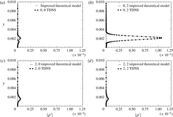
) is captured accurately by the model. The excellent agreement is further confirmed by figure 18, where the wall-normal amplitude distributions extracted at
 $t=1.0$
are compared. Having a closer look at the wall-normal amplitude distributions, it is worth noting the following observation. While large acoustic waves were present for the linear evolution of each disturbance, neither the superposition model nor the TDNS shows evidence of those acoustic waves. This implies that acoustic waves are cancelled out in the superposition process.
Comparison of the temporal development of the disturbance density maximum for the nonlinearly generated modes (
 $0,0$
), (
 $0,2$
), (
 $2,0$
) and (
 $2,2$
) (a–d), between TDNS and the improved theoretical model. Note that in each graph the TDNS mode that is compared to the improved theoretical model is plotted with solid symbols.

Comparison of the wall-normal amplitude distribution of the disturbance density for the nonlinearly generated modes (
 $0,0$
), (
 $0,2$
), (
 $2,0$
) and (
 $2,2$
) (a–d), between TDNS and the improved theoretical model.

The above results suggest that although the growth rates of the nonlinearly generated waves can be predicted by a purely nonlinear model, one has to account for the linear eigenbehaviour of the nonlinearly imposed disturbances to also predict the exact amplitudes. The main finding of this investigation is that the signature mode (
 $0,2$
) of oblique breakdown is at a significantly higher amplitude than the other nonlinearly generated modes, because its amplitude level is elevated by a constantly forced transient (or non-modal) growth. In other words, at each time step the primary pair of oblique waves acts as an ‘actuator’ and imposes non-modal unstable disturbances into mode (
 $0,2$
), which then are ultimately responsible for raising the amplitude level. Hence, the linear eigenbehaviour is also of significant importance in the nonlinear transition regime.
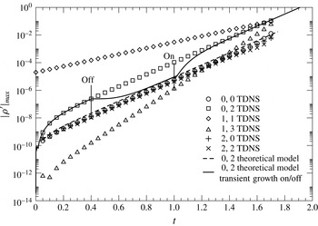
To further support these findings, the following thought experiment is explored. It is motivated by the question: what would happen to mode (
 $0,2$
) if the transient growth could be switched on and off? For this experiment the timeline prescribing the time intervals when the transient growth is switched on and off is given as
 $$\begin{eqnarray}\text{Transient growth }\left\{\begin{array}{@{}ll@{}}\text{on} & \text{for}~0.0\leqslant t<0.4,\\ \text{off} & \text{for}~0.4\leqslant t<1.0,\\ \text{on} & \text{for}~1.0\leqslant t\leqslant 2.0.\end{array}\right.\end{eqnarray}$$
As discussed previously, a model for the development of mode (
 $0,2$
) is readily available for both cases including and excluding transient growth. Therefore, the development according to the above timeline can be calculated by incorporating an additional term that accounts for the initial condition into (4.16) and (4.8). For the specific example, the evolution of the amplitude is given by
 $$\begin{eqnarray}\displaystyle \unicode[STIX]{x1D70C}_{0,2}^{\prime }(t(n))=\left\{\begin{array}{@{}ll@{}}\displaystyle \mathop{\sum }_{i=1}^{n}\unicode[STIX]{x1D70C}_{0,2,lin}(i)\text{e}^{2\unicode[STIX]{x1D70E}t(n-i+1)} & \text{for }1\leqslant n<n_{1},\\ \unicode[STIX]{x1D70C}_{0,2}^{\prime }(t(n_{1}))-{\displaystyle \frac{(A_{0}\text{e}^{\unicode[STIX]{x1D70E}(t(n_{1}))})^{2}}{8\unicode[STIX]{x1D70E}}}\hat{\unicode[STIX]{x1D70C}}_{0,2,nl}(y)(\text{e}^{2\unicode[STIX]{x1D70E}(t(n)-t(n_{1}))}-1) & \text{for }n_{1}\leqslant n<n_{2},\\ \displaystyle \unicode[STIX]{x1D70C}_{0,2}^{\prime }(t(n_{2}))+\mathop{\sum }_{i=1}^{n-n_{2}}\unicode[STIX]{x1D70C}_{0,2,lin}(i)\text{e}^{2\unicode[STIX]{x1D70E}t(n-n_{2}-i+1)} & \text{for }n_{2}\leqslant n\leqslant n_{3},\end{array}\right. & & \displaystyle \nonumber\\ \displaystyle & & \displaystyle\end{eqnarray}$$
where the same time array already used for (4.16) was incorporated with
 $n_{1}=40\,000$
(
 $t(n_{1})=0.4$
),
 $n_{2}=100\,000$
(
 $t(n_{2})=1.0$
) and
 $n_{3}=200\,000$
(
 $t(n_{3})=2.0$
). The result is presented in figure 19, where the solid line indicates the evolution of mode (
 $0,2$
) calculated with (4.19). Up to
 $t=0.4$
, the development of mode (
 $0,2$
) is identical to the development shown in figure 19. Then the transient growth is switched off at
 $t=0.4$
. As a result, the amplitude curve immediately levels off (zero slope) and asymptotically approaches the curve representing the purely nonlinear generation of mode (
 $0,2$
). Then at time
 $t=1.0$
the transient growth is turned on again and the amplitude curve experiences a sharp rise until it eventually falls back onto the amplitude curve from the TDNS in an asymptotic fashion. It is appropriate at this point to explain the evolution of the amplitude curve after both events, i.e. after the transient growth is switched off and after the transient growth is switched on, in more detail. The sharp kink at
 $t=0.4$
implies a discontinuity in the first derivative. That is due to the rather strong (unphysical) intervention of turning off any eigenbehaviour after
 $t=0.4$
. If the disturbances seeded prior to
 $t=0.4$
would be allowed to continue with their linear eigenbehaviour, the transition would be significantly smoother. After the transient growth is turned on again (at
 $t=1.0$
), the adjustment is also rather abrupt for similar reasons. The outcome of this experiment suggests that there are two theoretical amplitude levels: the first is due to purely nonlinear interaction, whereas the second is related to the nonlinear interaction combined with transient growth, which will be reached after a short adjustment period. This is also evidence for the fact that the amplitudes of the nonlinear generated modes do not depend on their initial amplitude, but only on the amplitude of the primary mode.
Thought experiment. What would happen if transient growth could be switched off and on?

5 Conclusion
A key feature of oblique breakdown is the dominance of the longitudinal mode (
 $0,2$
) in the early nonlinear regime. This has been known since the work of Fasel et al. (Reference Fasel, Thumm, Bestek, Kral and Zang1993) for a
 $M=1.6$
boundary layer and by Schmid & Henningson (Reference Schmid and Henningson1992) for an incompressible boundary layer, but the underlying physical mechanisms have never been fully explained. Using temporal simulations and theoretical considerations, it was shown that the high amplitude of this mode is due to a constantly forced transient growth mechanism. The primary pair of oblique waves (mode
 $1,1$
) hereby acts like an ‘actuator’, which is permanently seeding disturbances into mode (
 $0,2$
). Once seeded, these disturbances eventually exhibit a non-modal unstable behaviour that is ultimately responsible for raising the amplitude level of mode (
 $0,2$
). In contrast, the other modes from the first level of nonlinearly generated modes (modes
 $0,0$
,
 $2,0$
and
 $2,2$
), initially experience no growth, but decay instead. As a consequence, the amplitude levels of these modes are below the amplitude levels predicted by the simpler model that did not account for the linear eigenbehaviour of the nonlinearly generated disturbances. It is important to note that, on the other hand, the exponential growth rate of the nonlinearly generated modes is unaffected by their linear eigenbehaviour but is only a consequence of the nonlinear interactions. This finding is essential for making a connection to oblique transition (the incompressible counterpart of oblique breakdown), where transient growth was established to be the primary mechanism leading to turbulence. The difference between both scenarios is that in oblique transition, the nonlinearly generated mode (
 $0,2$
) exhibits transient growth by itself, whereas in oblique breakdown only the disturbances seeded into mode (
 $0,2$
) are non-modal unstable and the mode (
 $0,2$
) itself grows nonlinearly with twice the growth rate of the primary pair of oblique waves (mode
 $1,1$
). Therefore, transient growth does play an important role in the transition process of oblique breakdown even if the disturbances grow exponentially. Additionally, the same study demonstrated that after a certain time interval the amplitude of mode (
 $0,2$
) is independent of the initial amplitude of mode (
 $0,2$
). Hence the asymptotic state is solely determined by the amplitude of the primary pair of oblique waves. Thus, the research presented in this paper supports and confirms the conjecture by Schmid & Henningson (Reference Schmid and Henningson1992), that non-modal growth is responsible for the predominant role of the longitudinal mode in oblique breakdown.
Acknowledgements
This research was funded by the Supersonics Project of NASA’s Fundamental Aeronautics Program under cooperative agreement NNX07AC66A, with Dr M. Choudhari, NASA Langley Research Center, serving as the Technical Monitor and the AFOSR/NASA National Center of Hypersonic Laminar-Turbulent Transition Research at the Texas A&M University. The authors gratefully acknowledge the support of C. Hader in editing the paper.