1. Introduction
A wide range of physical problems, from nanophotonic crystals (Borisnika Reference Borisnika2006) and molecules (Creighton Reference Creighton1982) to giant stars (Lavely Reference Lavely1983), take place in tori or disks: they contain rotating symmetries and can therefore exhibit azimuthal/transverse oscillations such as electromagnetic waves (Pang, Tetz & Fainman Reference Pang, Tetz and Fainman2007), acoustic waves (Krebs et al.
Reference Krebs, Flohr, Prade and Hoffmann2002; Noiray, Bothien & Schuermans Reference Noiray, Bothien and Schuermans2011; Parmentier et al.
Reference Parmentier, Salas, Wolf, Staffelbach, Nicoud and Poinsot2012; Bauerheim et al.
Reference Bauerheim, Parmentier, Salas, Nicoud and Poinsot2014c
), surface waves (Feng & Sethna Reference Feng and Sethna1989; Simonelli & Gollub Reference Simonelli and Gollub1989), magnetostatic spin waves (i.e. propagating disturbances in the ordering of magnetic materials) (Hoffmann et al.
Reference Hoffmann, Woltersdorf, Perzlmaier, Slavin, Tiberkevich, Bischof, Weiss and Back2007; Guslienko et al.
Reference Guslienko, Slavin, Tiberkevich and Kim2008; Barman et al.
Reference Barman, Barman, Kimura, Fukuma and Otani2010; Kammerer et al.
Reference Kammerer, Weigand, Curcic, Sproll, Vansteenkiste, Waeyenberge, Stoll, Woltersdorf, Back and Schuetz2011) or solid vibrations (Perrin & Charnley Reference Perrin and Charnley1973; Creighton Reference Creighton1982; Lin & Parker Reference Lin and Parker2000a
,Reference Lin and Parker
b
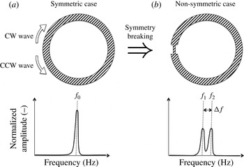
; Kumar & Krousgrill Reference Kumar and Krousgrill2012). When the rotating symmetry is perfect, these modes occur in doubly degenerate pairs with two independent oscillations (a clockwise (CW) and a counter-clockwise (CCW) wave) at the same frequency (figure 1
a). However, when systems with rotational symmetry are modified either in their geometry or by spatially varying their properties or their boundary conditions, degenerate pairs can split into two distinct modes with different yet close frequencies (figure 1
b). In some applications, the splitting frequency
 ${\rm\Delta}f$
can be fairly large and therefore cannot be ignored (e.g.
 ${\rm\Delta}f=0.25\ \text{GHz}$
for spin-wave modes in small ferromagnetic elements (Hoffmann et al.
Reference Hoffmann, Woltersdorf, Perzlmaier, Slavin, Tiberkevich, Bischof, Weiss and Back2007)).
(a) Sketch of a configuration with rotating symmetries (top) and its associated spectrum (bottom). Two waves (CW and CCW) can exist and have the same frequency
 $f_{0}$
: the mode is ‘degenerate’. When the rotating symmetry is broken (b), the degenerate mode at
 $f_{0}$
is split into two distinct waves with different yet close frequencies
 $f_{1}$
and
 $f_{2}$
(bottom).

In many applications, this splitting can lead to catastrophic effects, requiring studies to understand their underlying nature and methods to suppress them. For instance, photonic crystals (i.e. devices where several electromagnetic microcavities are coupled with a specific pattern to form ‘photon molecules’) with high quality factors are essential for the development of the next generation of optoelectronic components, but undesired symmetry breaking and associated non-degenerate modes reduce their overall performance. To tackle this problem, Borisnika (Reference Borisnika2006) proposed arrangement patterns with enhanced symmetry characteristics which reduce the effects of non-degenerate modes and improve the quality factors of the devices.
In applications based on magnetic disks which exhibit spin waves (Hoffmann et al. Reference Hoffmann, Woltersdorf, Perzlmaier, Slavin, Tiberkevich, Bischof, Weiss and Back2007; Guslienko et al. Reference Guslienko, Slavin, Tiberkevich and Kim2008; Barman et al. Reference Barman, Barman, Kimura, Fukuma and Otani2010; Kammerer et al. Reference Kammerer, Weigand, Curcic, Sproll, Vansteenkiste, Waeyenberge, Stoll, Woltersdorf, Back and Schuetz2011), theoretical models show that the splitting is a consequence of the interaction of the azimuthal mode with the vortex-core gyrotropic motion. Both simulations and experiments have confirmed that removing the vortex core from the disk suppresses mode splitting (Hoffmann et al. Reference Hoffmann, Woltersdorf, Perzlmaier, Slavin, Tiberkevich, Bischof, Weiss and Back2007). This suggests that theory, simulations or experiments can unveil the splitting origins and offer methods to suppress them.
In configurations where symmetry breaking is well described theoretically (Mazzei et al. Reference Mazzei, Gotzinger, Menezes, Zumofen, Benson and Sandoghdar2007), scientists can readily perform symmetry breaking to analyse the phenomenon responsible for this splitting. For example, in ultra-high-quality-factor whispering-gallery-mode resonators (WGMs), a small imperfection (similar to the case b in figure 1) or a deposited particle can scatter light from one of the two cavity modes (CCW for instance) into free space as well as in the opposite direction (i.e. CW). Scientists can then exploit this splitting to accurately determine particle sizes (Mazzei et al. Reference Mazzei, Gotzinger, Menezes, Zumofen, Benson and Sandoghdar2007; Kippenberg Reference Kippenberg2010). A similar methodology is used in helioseismology (Lavely Reference Lavely1983; Kosovichev Reference Kosovichev1999; Tripathy, Jain & Bhatnagar Reference Tripathy, Jain and Bhatnagar2000), where the internal solar structure and dynamics can be inferred from observed frequencies which can be split by either rotation, asphericity or the magnetic field of the star.
In the particular field of fluid mechanics, symmetry breaking phenomena are less studied due to complex geometries, high nonlinear levels and complex physics. In simple configurations (square and quasi-square channels), such a splitting effect has been studied for surface waves (Feng & Sethna Reference Feng and Sethna1989; Simonelli & Gollub Reference Simonelli and Gollub1989). Results show that the symmetry of the configuration has dramatic effects on the dynamics. The degenerate case yields no time-dependent patterns. However, set-ups where the two components are separated in frequency, even by a small amount (approximately 1 %), can lead to chaotic states (Simonelli & Gollub Reference Simonelli and Gollub1989). Similarly, Davey et al. (Davey & Salwen Reference Davey and Salwen1994) investigated the linear stability of the first circumferential mode in both a circular and an elliptic pipe. They showed analytically that the circular problem has a doubly degenerate eigenvalue
 $f_{0}$
while the ellipticity of the latter configuration splits the doublets into two distinct eigenvalues
 $f_{0}\pm {\rm\Delta}f/2$
. The imaginary part of the splitting frequency
 ${\rm\Delta}f$
is non-zero and thus the ellipticity of the cross-sectional area always makes the flow less stable. This splitting mechanism induced by the symmetry reduction (from the axisymmetry group
 $S^{1}$
of the circular problem to the mirror symmetry group
 $Z_{2}$
associated with the elliptic cross-section) is briefly discussed in its fundamental mathematical aspects in Guckenheimer & Mahalov (Reference Guckenheimer and Mahalov1992) and applied to the instability of a vortex filament in a non-circular cylinder. Such a symmetry reduction also plays a crucial role on the oscillations of droplets due to asphericity (Cummings & Blackburn Reference Cummings and Blackburn1991) and/or Coriolis forces if the droplet is rotating (Busse Reference Busse1984).
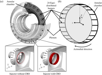
Recently, symmetry breaking has also been investigated in complex annular gas turbines (figure 2) (Noiray et al. Reference Noiray, Bothien and Schuermans2011; Parmentier et al. Reference Parmentier, Salas, Wolf, Staffelbach, Nicoud and Poinsot2012), which exhibit azimuthal acoustic waves produced by thermo-acoustic instabilities (O’Connor & Lieuwen Reference O’Connor and Lieuwen2014). Such combustion instabilities remain a severe problem in the development of modern gas turbines. Lean premixed combustors, designed to reduce nitric oxide emissions significantly, are especially prone to these oscillations which can lead to vibrations and structural damage (Krebs et al. Reference Krebs, Flohr, Prade and Hoffmann2002; Schuermans, Bellucci & Paschereit Reference Schuermans, Bellucci and Paschereit2003; Lieuwen & Yang Reference Lieuwen and Yang2005). These unsteady phenomena come from the interaction between acoustics and heat-release fluctuations which act as a volume acoustic source (Strahle Reference Strahle1972). In annular combustion chambers (figure 2), these instabilities often take the form of azimuthal modes (Krebs et al. Reference Krebs, Flohr, Prade and Hoffmann2002; Schuermans et al. Reference Schuermans, Bellucci and Paschereit2003; Parmentier et al. Reference Parmentier, Salas, Wolf, Staffelbach, Nicoud and Poinsot2012; Worth & Dawson Reference Worth and Dawson2013a ,Reference Worth and Dawson b ; Bauerheim et al. Reference Bauerheim, Parmentier, Salas, Nicoud and Poinsot2014c ).
(a) A typical 3D configuration of an industrial annular combustion chamber equipped with a number
 $N=24$
of burners with or without cylindrical burner outlets (CBOs) and (b) network model of the annular chamber (—–) with
 $N=24$
burners. The annular plenum (- - -) is removed for the sake of simplicity.

In real engines, usually, identical burners are distributed regularly along the azimuthal direction (figure 2). Therefore, perfectly axisymmetric configurations have been intensively investigated using theoretical (Stow & Dowling Reference Stow and Dowling2001; Pankiewitz & Sattelmayer Reference Pankiewitz and Sattelmayer2003; Stow & Dowling Reference Stow and Dowling2003; Parmentier et al. Reference Parmentier, Salas, Wolf, Staffelbach, Nicoud and Poinsot2012; Bauerheim et al. Reference Bauerheim, Parmentier, Salas, Nicoud and Poinsot2014c ), acoustic and large eddy simulation (LES) tools (Evesque & Polifke Reference Evesque and Polifke2002; Kopitz et al. Reference Kopitz, Huber, Sattelmayer and Polifke2005; Staffelbach et al. Reference Staffelbach, Gicquel, Boudier and Poinsot2009; Wolf et al. Reference Wolf, Staffelbach, Gicquel, Muller and Poinsot2012) and more rarely experiments (Krebs et al. Reference Krebs, Flohr, Prade and Hoffmann2002; Bourgouin et al. Reference Bourgouin, Durox, Moeck, Schuller and Candel2013; Worth & Dawson Reference Worth and Dawson2013a ,Reference Worth and Dawson b ). Annular chambers exhibit specific azimuthal modes which can be standing or spinning in the azimuthal direction (Evesque, Polifke & Pankiewitz Reference Evesque, Polifke and Pankiewitz2003; Sensiau, Nicoud & Poinsot Reference Sensiau, Nicoud and Poinsot2009). Azimuthal modes are often ‘degenerate’: two modes are found at the same frequency (two counter-rotating spinning modes, for example). These two modes can combine and switch, leading to combustors that exhibit standing, spinning or mixed modes for various times, changing from one mode to another one at random instants. The simultaneous existence of these modes has been observed numerically (Wolf et al. Reference Wolf, Staffelbach, Gicquel, Muller and Poinsot2012) and experimentally in laboratory set-ups (Bourgouin et al. Reference Bourgouin, Durox, Moeck, Schuller and Candel2013; Worth & Dawson Reference Worth and Dawson2013b ) and even in real gas turbines (Krebs et al. Reference Krebs, Flohr, Prade and Hoffmann2002). Mode switching has been postulated to be due to random turbulent fluctuations (Noiray & Schuermans Reference Noiray and Schuermans2013). Azimuthal modes are not necessarily degenerate, leading to a more complicated situation where the configuration is strongly affected by symmetry modifications, as shown by studies of sound produced by bells (Perrin & Charnley Reference Perrin and Charnley1973), where non-degenerate but very close azimuthal modes (also called ‘non-degenerate singlets’) lead to ‘warble’, an undesired modulation due to the coupling of two modes with different but very close frequencies.
The effect of asymmetry on the eigenfrequencies and nature of azimuthal modes in annular chambers is still an open question. Earlier work by Oefelein & Yang (Reference Oefelein and Yang1993) focused on symmetry breaking using baffles to prevent combustion instabilities in the F-1 rocket engines. They suggested that asymmetry can be introduced to control unstable modes using passive techniques. Stow & Dowling (Reference Stow and Dowling2003) applied azimuthal variations using Helmholtz resonators on an annular academical test bench. Similarly, Krueger et al. (Reference Krueger, Hueren, Hoffmann, Krebs, Flohr and Bohn2000) and Berenbrink & Hoffmann (Reference Berenbrink and Hoffmann2001) (reviewed by Culick & Kuentzmann (Reference Culick and Kuentzmann2006)) broke the symmetry of an annular engine by using CBOs (figure 2
a, bottom) to modify the time delay
 ${\it\tau}_{i}$
of some of the 24 flames and control instabilities in an
 $N=24$
burner industrial combustor. They varied the number of CBOs installed among the 24 burners, showing that the addition of CBOs improved stability. However, it was not clear whether the stabilization was due to the CBO devices rather than, as argued by the authors, symmetry breaking in this particular case. Recently, Moeck, Paul & Paschereit (Reference Moeck, Paul and Paschereit2010) and Gelbert et al. (Reference Gelbert, Moeck, Paschereit and King2012) carried out an annular Rijke experiment with heating grids acting like flames. They introduced circumferential variations through asymmetric power distributions of the grids to modify the azimuthal mode behaviour and noticed that the staging pattern can split degenerate azimuthal modes (doublets) into non-degenerate pairs (singlets), as suggested in Perrin & Charnley (Reference Perrin and Charnley1973) for bells, if the system’s symmetry is changed. Recently, experimental (Worth & Dawson Reference Worth and Dawson2013a
,Reference Worth and Dawson
b
) and theoretical (Bauerheim, Cazalens & Poinsot Reference Bauerheim, Cazalens and Poinsot2014a
) studies have shown that the azimuthal flow itself can break the rotating symmetry. This flow gyration can be generated by the compressor or diffuser outlet, by the swirlers or even by effusive plates in modern gas turbines. Worth & Dawson (Reference Worth and Dawson2013a
,Reference Worth and Dawson
b
) have shown that changing the rotating direction of some swirlers can modify the stability and the structure of the observed acoustic mode. This mean flow effect has been analytically unveiled by Bauerheim et al. (Reference Bauerheim, Cazalens and Poinsot2014a
), demonstrating that the mean azimuthal Mach number is one parameter controlling the symmetry breaking affecting both the stability and the mode nature.
A few theories consider the effect of asymmetry on the existence and nature of azimuthal modes (standing, spinning or mixed). Schuermans, Paschereit & Monkewitz (Reference Schuermans, Paschereit and Monkewitz2006) suggested that standing modes are observed for low amplitudes but that, at higher amplitudes, one of the two rotating modes eventually dominates. However, Sensiau et al. (Reference Sensiau, Nicoud and Poinsot2009) have shown that even in the linear regime, any change in symmetry can lead to the appearance of one rotating mode dominating the other one: when the symmetry of the configuration is broken, the standing azimuthal mode is changed into two counter-rotating azimuthal modes with different growth rates so that one of them eventually dominates the other. Noiray et al. (Reference Noiray, Bothien and Schuermans2011) have proved that the
 $2p$
th Fourier coefficient of the heat release, temperature or even acoustic loss azimuthal distribution (where
 $p$
is the order of the azimuthal mode considered) strongly impacts the frequency as well as the mode nature on an annular rig. Dawson et al. (Worth & Dawson Reference Worth and Dawson2013a
,Reference Worth and Dawson
b
) have also shown that the mode nature can result from the interaction with the mean flow by breaking symmetry thanks to CW/CCW swirlers: they observed a strong correlation between the bulk swirl direction and the direction of spin.
Noiray et al. (Reference Noiray, Bothien and Schuermans2011) used an analytical formulation to study the effect of asymmetry on a annular rig with a circumferential distribution of heat release, temperature and acoustic losses. However, for the sake of simplicity, this annular rig was simplified and contained no burner at all: no study was conducted on annular chambers connected to burners, a configuration which is more realistic for real gas turbines but more difficult to formulate analytically.
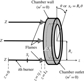
The present paper describes an analytical approach to investigate the effects of symmetry breaking on azimuthal modes in an annular chamber fed by
 $N$
identical or non-identical burners. This configuration, called BC (burner
 $+$
chamber, figure 3), allows the investigation of the effect of asymmetry on eigenfrequencies and the nature of circumferential modes. The model is based on a network description (figure 2) of the combustion chamber where only plane acoustic waves travel and interact with flames (Parmentier et al.
Reference Parmentier, Salas, Wolf, Staffelbach, Nicoud and Poinsot2012). It allows one to take into account the effects of burners and of complex flame models while providing a solution that remains almost fully analytical. This analytical formulation reveals which parameters control the growth and the nature of the modes, something which would be impossible with a numerical approach.
The BC configuration to study unstable modes in annular chambers.

This paper is organized as follows. Section 2 briefly describes the principle of the acoustic network model called ‘analytical tool to analyse and control azimuthal modes in annular combustors’ (ATACAMAC) and how an analytical dispersion relation can be obtained in such a configuration (Parmentier et al.
Reference Parmentier, Salas, Wolf, Staffelbach, Nicoud and Poinsot2012). In § 3, analytical calculations of eigenfrequencies are presented for both an ‘unperturbed’ case (an annular cavity without flames) and a general non-symmetric BC configuration (figure 3). Section 4 describes the test cases as well as the 3D Helmholtz solver used to validate the ATACAMAC results. Two application cases are presented: an academic chamber with
 $N=3$
burners and a real configuration with
 $N=24$
burners (figure 2). In § 5, ATACAMAC is applied to a BC configuration with
 $N=3$
identical burners (§ 5.1) and then
 $N=3$
different burners (§ 5.2), highlighting the effect of circumferential patterns on eigenfrequencies and mode nature. ATACAMAC results are systematically compared with those provided by a 3D acoustic code solving the complete acoustic equations in three dimensions in the low-Mach-number case (Selle et al.
Reference Selle, Benoit, Poinsot, Nicoud and Krebs2006; Nicoud et al.
Reference Nicoud, Benoit, Sensiau and Poinsot2007; Sensiau et al.
Reference Sensiau, Nicoud and Poinsot2009; Silva et al.
Reference Silva, Nicoud, Schuller, Durox and Candel2013). Finally, § 6 presents the effects of asymmetry on instabilities in an
 $N=24$
burner configuration typical of real engines. The results are compared with observations made in real gas turbine engines (Krueger et al.
Reference Krueger, Hueren, Hoffmann, Krebs, Flohr and Bohn2000; Berenbrink & Hoffmann Reference Berenbrink and Hoffmann2001).
2. A network model for a BC non-symmetric configuration
2.1. Model description
This study focuses on a BC configuration where an annular chamber is fed by
 $N$
burners (figure 3). An impedance
 $Z$
is imposed at the upstream end of each burner. The mean density and sound speed are denoted
 ${\it\rho}^{0}$
and
 $c^{0}$
in the annular chamber and
 ${\it\rho}_{u}^{0}$
and
 $c_{u}^{0}$
for the unburnt mixture in the
 $N$
burners. The perimeter and the cross-sectional area (perpendicular to the azimuthal direction) of the annular chamber are denoted
 $2L_{c}=2{\rm\pi}R_{c}$
and
 $S_{c}$
respectively. The length and section of the
 $i$
th burner are
 $L_{i}$
and
 $S_{i}$
. The position along the annular cavity is given by the angle
 ${\it\theta}$
, defining an abscissa
 $x_{c}=R_{c}{\it\theta}$
. The location of the flame is similar in all burners and is given by the normalized abscissa
 ${\it\alpha}=z_{f,i}/L_{i}$
(figure 3).
This model corresponds to situations where pressure fluctuations in the combustion chamber depend on the angle
 ${\it\theta}$
(or the azimuthal position
 $x$
) but not on the axial direction
 $z$
in the chamber (they depend on the coordinate
 $z$
only in the burners). This case can be observed in combustors terminated by choked nozzles which acoustically behave almost like a rigid wall (i.e.
 $u^{\prime }=0$
under the low-upstream-Mach-number assumption (Marble & Candel Reference Marble and Candel1977)). Since the chamber inlet is also close to a velocity node, modes which have no variation along
 $z$
can develop in the chamber, as shown by recent LES in real engines (Wolf et al.
Reference Wolf, Staffelbach, Roux, Gicquel, Poinsot and Moureau2009).
The model provides the analytical expression of eigenfrequencies for a general asymmetric case for any mode order
 $p$
and any number of burners
 $N$
as well as general rules on stability for annular combustors. Results on the structure and nature of azimuthal modes (spinning, standing or mixed) will be derived using this analytical study to show how asymmetry can promote specific modes and control instabilities (Moeck et al.
Reference Moeck, Paul and Paschereit2010; Noiray et al.
Reference Noiray, Bothien and Schuermans2011; Gelbert et al.
Reference Gelbert, Moeck, Paschereit and King2012; Worth & Dawson Reference Worth and Dawson2013a
,Reference Worth and Dawson
b
).
2.2. Annular network reduction
Network models that account for one annular cavity connected to
 $N$
burners usually require a large number of unknown variables (acoustic pressure and velocity in each network tube) and a large matrix describing the system (typically a
 $2N\times 2N$
matrix). To reduce the size of the system (i.e. a matrix of size
 $2\times 2$
, independent of the number
 $N$
of burners), the ANR (annular network reduction) methodology proposed in Bauerheim et al. (Reference Bauerheim, Parmentier, Salas, Nicoud and Poinsot2014c
) is applied: the full annular combustor is split into
 $N$
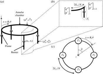
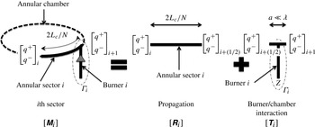
sectors which differ only in the burner/chamber junction (figures 4 and 5). Between each sector, the propagation of azimuthal waves (along
 ${\it\theta}$
or
 $x$
) can be modelled by a transfer matrix
 $\unicode[STIX]{x1D64D}_{i}$
, as proposed by Parmentier et al. (Reference Parmentier, Salas, Wolf, Staffelbach, Nicoud and Poinsot2012) (figure 5, propagation),
 $$\begin{eqnarray}\left[\begin{array}{@{}c@{}}q^{+}\\ q^{-}\end{array}\right]_{i+1/2}=\left[\begin{array}{@{}c@{}}\unicode[STIX]{x1D64D}_{i}\end{array}\right]\left[\begin{array}{@{}c@{}}q^{+}\\ q^{-}\end{array}\right]_{i},\quad \text{where}\;\left[\begin{array}{@{}c@{}}\unicode[STIX]{x1D64D}_{i}\end{array}\right]=\left[\begin{array}{@{}cc@{}}W & 0\\ 0 & \displaystyle \frac{1}{W}\end{array}\right].\end{eqnarray}$$
Here,
 $q^{\pm }=p^{\prime }\pm {\it\rho}^{0}c^{0}u^{\prime }$
,
 $W=\text{e}^{2jkL_{c}/N}$
and the wavenumber
 $k={\it\omega}/c^{0}$
.
3D view of a BC configuration with
 $N=4$
burners (a), zoom on the
 $i$
th sector (b) and model of the whole BC configuration (c), where
 ${\rm\Gamma}_{i}$
represents the burner/chamber interaction (Parmentier et al.
Reference Parmentier, Salas, Wolf, Staffelbach, Nicoud and Poinsot2012).

The ANR methodology: each sector is decomposed into a free propagation of azimuthal waves (characteristic length
 $2L_{c}/N$
) and a compact burner/chamber interaction (characteristic length
 $a\ll {\it\lambda}$
) modelled by the coupling parameter
 ${\rm\Gamma}_{i}$
.

The area where the
 $i$
th burner is connected to the annular chamber (- - - in figure 4
b) was investigated by O’Connor et al. (O’Connor & Lieuwen Reference O’Connor and Lieuwen2012a
,Reference O’Connor and Lieuwen
b
,Reference O’Connor and Lieuwen
c
) and can be assumed to be compact:
 $a\ll {\it\lambda}$
, where
 $a=2\sqrt{S_{i}/{\rm\pi}}$
is the burner diameter and
 ${\it\lambda}=2L_{c}/p$
is the acoustic wavelength, leading to the compactness criterion
 $p\ll L_{c}\sqrt{{\rm\pi}/S_{c}}\simeq 116$
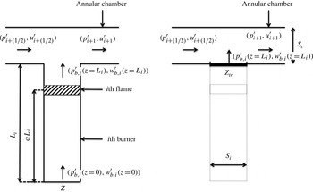
. As shown in figure 6, using the equations of acoustic propagation in the cold (
 $0<z<{\it\alpha}L_{i}$
) and hot (
 ${\it\alpha}L_{i}<z<L_{i}$
) parts of the burner as well as the jump conditions through the
 $i$
th flame (
 $z={\it\alpha}L_{i}$
), the effect of the whole
 $i$
th burner on the annular chamber can be obtained by a translated impedance from
 $z=0$
(impedance
 $Z$
) to the burner/chamber junction at
 $z=L_{i}$
(impedance
 $Z_{tr}=(p_{b,i}^{\prime }(z=L_{i})/{\it\rho}^{0}c^{0}w_{b,i}^{\prime }(z=L_{i}))$
(Blimbaum et al.
Reference Blimbaum, Zanchetta, Akin, Acharya, O’Connor, Noble and Lieuwen2012; Bauerheim et al.
Reference Bauerheim, Parmentier, Salas, Nicoud and Poinsot2014c
):
 $$\begin{eqnarray}Z_{tr}=\frac{\mathbb{F}S_{1-{\it\alpha}}^{k}[\,jC_{{\it\alpha}}^{k_{u}}-S_{{\it\alpha}}^{k_{u}}Z]+C_{1-{\it\alpha}}^{k}[C_{{\it\alpha}}^{k_{u}}Z+jS_{{\it\alpha}}^{k_{u}}]}{\mathbb{F}C_{1-{\it\alpha}}^{k}[\,jS_{{\it\alpha}}^{k_{u}}Z+C_{{\it\alpha}}^{k_{u}}]+S_{1-{\it\alpha}}^{k}[\,jC_{{\it\alpha}}^{k_{u}}Z-S_{{\it\alpha}}^{k_{u}}]},\end{eqnarray}$$
where
 $\mathbb{F}=({\it\rho}^{0}c^{0}/{\it\rho}_{u}^{0}c_{u}^{0})(1+n_{i}\text{e}^{\,j{\it\omega}{\it\tau}_{i}})$
, the notations for the sine and cosine functions are
 $C_{{\it\alpha}}^{k_{u}}=\cos ({\it\alpha}k_{u}L_{i}),S_{{\it\alpha}}^{k_{u}}=\sin ({\it\alpha}k_{u}L_{i}),C_{1-{\it\alpha}}^{k}=\cos ((1-{\it\alpha})kL_{i}),S_{1-{\it\alpha}}^{k}=\sin ((1-{\it\alpha})kL_{i})$
and the wavenumbers are
 $k={\it\omega}/c^{0}$
and
 $k_{u}={\it\omega}/c_{u}^{0}$
. It should be noted that the
 $n$
–
 ${\it\tau}$
model can be replaced by more complex flame descriptions such as flame describing functions (FTFs) (Noiray et al.
Reference Noiray, Durox, Schuller and Candel2008) or transfer matrices (Polifke et al.
Reference Polifke, Poncet, Paschereit and Doebbeling2001).
Equivalent impedance of the whole
 $i$
th burner (which includes the
 $i$
th active flame) near the burner/chamber interaction zone (figure 5). The translated impedance
 $Z_{tr}$
at
 $z=L_{i}$
takes into account the upstream impedance
 $Z$
at
 $z=0$
, the propagation in the cold (
 $0<z<{\it\alpha}L_{i}$
) and hot (
 ${\it\alpha}L_{i}<z<L_{i}$
) parts of the burner as well as the active flame effect via the FTF (
 $n_{i},{\it\tau}_{i}$
).

The jump conditions at the burner/chamber junction at null Mach number read (Davies Reference Davies1988; Dowling Reference Dowling1995; Poinsot & Veynante Reference Poinsot and Veynante2011; Bauerheim, Nicoud & Poinsot Reference Bauerheim, Nicoud and Poinsot2014b )
 $$\begin{eqnarray}\displaystyle & \displaystyle p_{i+1/2}^{\prime }=p_{i+1}^{\prime }=p_{b,i}^{\prime }(z=L_{i}) & \displaystyle\end{eqnarray}$$
 $$\begin{eqnarray}\displaystyle & \displaystyle u_{i+1/2}^{\prime }S_{c}+\underbrace{w_{b,i}^{\prime }(z=L_{i})}_{=\frac{p_{i+1/2}^{\prime }}{{\it\rho}^{0}c^{0}Z_{tr}}}S_{i}=u_{i+1}^{\prime }S_{c}. & \displaystyle\end{eqnarray}$$
Consequently, a transfer matrix
 $\unicode[STIX]{x1D64F}_{i}^{\ast }$
for the interaction part of figure 5 can be deduced:
 $$\begin{eqnarray}\left[\begin{array}{@{}c@{}}p^{\prime }\\ {\it\rho}^{0}c^{0}u^{\prime }\end{array}\right]_{i+1}=\left[\begin{array}{@{}c@{}}\unicode[STIX]{x1D64F}_{i}^{\ast }\end{array}\right]\left[\begin{array}{@{}c@{}}p^{\prime }\\ {\it\rho}^{0}c^{0}u^{\prime }\end{array}\right]_{i+1/2}=\left[\begin{array}{@{}cc@{}}1 & 0\\ 2j{\rm\Gamma}_{i} & 1\end{array}\right]\left[\begin{array}{@{}c@{}}p^{\prime }\\ {\it\rho}^{0}c^{0}u^{\prime }\end{array}\right]_{i+1/2},\end{eqnarray}$$
where the coupling parameter
 ${\rm\Gamma}_{i}$
(Palies Reference Palies2010; Parmentier et al.
Reference Parmentier, Salas, Wolf, Staffelbach, Nicoud and Poinsot2012; Schuller et al.
Reference Schuller, Durox, Palies and Candel2012; Bauerheim et al.
Reference Bauerheim, Parmentier, Salas, Nicoud and Poinsot2014c
) (figure 5, burner/chamber interaction) is directly linked to the equivalent admittance
 $1/Z_{tr}$
of the whole
 $i$
th burner:
 $$\begin{eqnarray}{\rm\Gamma}_{i}=-\frac{j}{2}\frac{S_{i}}{S_{c}Z_{tr}}.\end{eqnarray}$$
When a velocity node (
 $Z=\infty$
) or a pressure node (
 $Z=0$
) is imposed at the upstream end of each burner and flames are located at the burner/chamber junction (
 ${\it\alpha}=1$
), the coupling parameters
 ${\rm\Gamma}_{i}$
reduce to (using (2.2) and (2.6))
 $$\begin{eqnarray}{\rm\Gamma}_{i}=\frac{1}{2}\frac{S_{i}{\it\rho}^{0}c^{0}}{S_{c}{\it\rho}_{u}^{0}c_{u}^{0}}\tan (k_{u}L_{i})\left(1+n_{i}\text{e}^{\,j{\it\omega}{\it\tau}_{i}}\right)\quad \text{when }Z=\infty\end{eqnarray}$$
or
 $$\begin{eqnarray}{\rm\Gamma}_{i}=-\frac{1}{2}\frac{S_{i}{\it\rho}^{0}c^{0}}{S_{c}{\it\rho}_{u}^{0}c_{u}^{0}}\;\text{cotan}(k_{u}L_{i})\left(1+n_{i}\text{e}^{\,j{\it\omega}{\it\tau}_{i}}\right)\quad \text{when }Z=0,\end{eqnarray}$$
where
 $k_{u}={\it\omega}/c_{u}$
and
 $(n_{i},{\it\tau}_{i})$
are the interaction index and the time delay of the FTF for the
 $i$
th flame (Crocco Reference Crocco1951). It should be noted that the coupling term in (2.5) is
 $2j{\rm\Gamma}_{i}p_{i+1/2}^{\prime }$
, thus burners and flames located at a pressure node have no effect on the acoustic mode, except in specific situations where
 ${\rm\Gamma}_{i}$
takes infinite values. For instance,
 ${\rm\Gamma}_{i}\rightarrow \infty$
in (2.8) when the burner length
 $L_{i}$
goes to zero. This corresponds to the Blimbaum exception case (Blimbaum et al.
Reference Blimbaum, Zanchetta, Akin, Acharya, O’Connor, Noble and Lieuwen2012) where the burner impedance attempts to force a pressure node at the burner/chamber junction. These specific situations require 3D acoustic considerations and are out of the scope of this study: since
 ${\rm\Gamma}_{i}\rightarrow \infty$
, the low-coupling-factor assumption
 $\Vert {\rm\Gamma}_{i}\Vert \ll 1$
(further described in (3.3)) is not satisfied meaning that no analytical solution can be provided.
Finally, (2.5) can be recast to relate characteristic waves
 $q^{\pm }=p^{\prime }\pm {\it\rho}^{0}c^{0}u^{\prime }$
instead of primitive variables
 $p^{\prime }$
and
 $u^{\prime }$
leading to the scattering matrix
 $\unicode[STIX]{x1D64F}_{i}$
:
 $$\begin{eqnarray}\left[\begin{array}{@{}c@{}}q^{+}\\ q^{-}\end{array}\right]_{i+1}=\left[\begin{array}{@{}c@{}}\unicode[STIX]{x1D64F}_{i}\end{array}\right]\left[\begin{array}{@{}c@{}}q^{+}\\ q^{-}\end{array}\right]_{i+1/2},\quad \text{where }\left[\begin{array}{@{}c@{}}\unicode[STIX]{x1D64F}_{i}\end{array}\right]=\left[\begin{array}{@{}cc@{}}1+j{\rm\Gamma}_{i} & j{\rm\Gamma}_{i}\\ -j{\rm\Gamma}_{i} & 1-j{\rm\Gamma}_{i}\end{array}\right].\end{eqnarray}$$
The waves at both ends of the
 $i$
th sector are connected by the
 $\unicode[STIX]{x1D648}_{i}=\unicode[STIX]{x1D64F}_{i}\unicode[STIX]{x1D64D}_{i}$
scattering matrix using (2.1) and (2.9) (figure 5):
 $$\begin{eqnarray}\left[\begin{array}{@{}c@{}}q^{+}\\ q^{-}\end{array}\right]_{i+1}=\left[\begin{array}{@{}c@{}}\unicode[STIX]{x1D64F}_{i}\end{array}\right]\left[\begin{array}{@{}c@{}}q^{+}\\ q^{-}\end{array}\right]_{i+1/2}=\underbrace{\left[\begin{array}{@{}c@{}}\unicode[STIX]{x1D64F}_{i}\end{array}\right]\left[\begin{array}{@{}c@{}}\unicode[STIX]{x1D64D}_{i}\end{array}\right]}_{\unicode[STIX]{x1D648}_{i}}\left[\begin{array}{@{}c@{}}q^{+}\\ q^{-}\end{array}\right]_{i}.\end{eqnarray}$$
Use of the periodicity condition
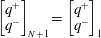 $\left[\begin{array}{@{}c@{}}q^{+}\\ q^{-}\end{array}\right]_{N+1}=\left[\begin{array}{@{}c@{}}q^{+}\\ q^{-}\end{array}\right]_{1}$
and (2.10) leads to
 $$\begin{eqnarray}\left(\mathop{\prod }\limits_{i=N}^{1}\unicode[STIX]{x1D648}_{i}\right)\left[\begin{array}{@{}c@{}}q^{+}\\ q^{-}\end{array}\right]_{1}=\left[\begin{array}{@{}c@{}}q^{+}\\ q^{-}\end{array}\right]_{1}.\end{eqnarray}$$
The system defined by (2.11) has non-trivial solutions only if its determinant is null. Therefore, the ANR methodology provides an implicit analytical dispersion relation for the pulsation
 ${\it\omega}$
for a general non-symmetric BC configuration:
 $$\begin{eqnarray}\det \left(\mathop{\prod }\limits_{i=N}^{1}\unicode[STIX]{x1D648}_{i}-\unicode[STIX]{x1D644}_{d}\right)=0,\end{eqnarray}$$
where
 $\unicode[STIX]{x1D644}_{d}$
is the
 $2\times 2$
identity matrix.
3. Analytical calculation of eigenfrequencies and mode structures
The analytical dispersion relation (2.12) provides the frequencies and the structure of the modes of the annular chamber. It allows the study of symmetry breaking by investigating the effects of the
 $N$
burner responses (modelled by the
 $N$
parameters
 ${\rm\Gamma}_{i},i\in [1,N]$
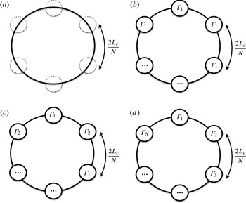
defined by (2.6)) on the growth rate and the nature of the azimuthal modes. Several configurations are considered here (figure 7) to understand the effect of symmetry breaking on combustion instabilities.
Typical configurations: unperturbed (a), symmetric with identical burners (b), pseudo-symmetric configuration (c) and the general non-symmetric configuration (d).

3.1. Unperturbed annular cavity (without burners and flames)
First, an annular chamber with no burner (i.e.
 ${\rm\Gamma}_{i}=0$
, for all
 $i\in [1,N]$
) is studied as a reference case (figure 7
a). The sound speed field corresponds to a reactive case:
 $c=c^{0}$
in the annular chamber. The transfer matrix of each sector (2.10) reduces to
 $\unicode[STIX]{x1D648}_{i}=\unicode[STIX]{x1D64D}_{i}$
since
 $\unicode[STIX]{x1D64F}_{i}=\unicode[STIX]{x1D644}_{d}$
: only azimuthal propagation occurs. Consequently (2.11) reduces to
 $$\begin{eqnarray}\left[\begin{array}{@{}cc@{}}W^{N} & 0\\ 0 & \displaystyle \frac{1}{W^{N}}\end{array}\right]\left[\begin{array}{@{}c@{}}q^{+}\\ q^{-}\end{array}\right]_{1}=\left[\begin{array}{@{}c@{}}q^{+}\\ q^{-}\end{array}\right]_{1}.\end{eqnarray}$$
The dispersion relation is therefore
 $W^{N}=1$
, where
 $W=\text{e}^{2jkL_{c}/N}$
. The
 $N$
solutions of (3.1) are
 $W_{0}=\text{e}^{2jp{\rm\pi}/N}$
and correspond to real eigenfrequencies of the unperturbed problem:
 $$\begin{eqnarray}kL_{c}=p{\rm\pi},\quad \text{so that }f=\frac{pc^{0}}{2L_{c}},\text{ for all }p\in \mathbb{N}.\end{eqnarray}$$
As expected, (3.2) corresponds to a family of azimuthal modes where the first one (
 $p=1$
) is the first azimuthal mode at frequency
 $c^{0}/2L_{c}$
which is the mode observed in many practical cases. Equation (3.1) also provides the eigenvectors
 $V$
associated with the eigenfrequencies
 $f$
given by (3.2). In this situation, the generated eigenspace
 $\{V\}$
is two-dimensional: all azimuthal modes are degenerate and can be either standing, spinning or mixed. All modes are neutral since no acoustic dissipation is included (zero growth rate:
 $\text{Im}(\,f)=0$
).
3.2. Non-symmetric BC configuration with active flames in the low-coupling limit
The use of a combustor with non-identical burners is a promising approach for the control of azimuthal modes (figure 7
d). An asymptotic expansion of the dispersion relation (2.12) can be used to study this case. Since all burners can be different, all coupling parameters
 ${\rm\Gamma}_{i}$
(2.6) can be different. A fully analytical solution can be formulated when the solution is ‘close’ to the unperturbed annular cavity case of § 3.1. This is obtained by assuming small coupling parameters
 ${\rm\Gamma}_{i}$
:
 $$\begin{eqnarray}{\rm\Gamma}_{i}\ll 1,\quad \text{for all }i\in [1,N].\end{eqnarray}$$
Under this assumption, a Taylor expansion of the transfer matrix of the whole system (
 $\unicode[STIX]{x1D648}=\prod _{i=N}^{1}\unicode[STIX]{x1D64F}_{i}\unicode[STIX]{x1D64D}_{i}$
) at second order gives
 $$\begin{eqnarray}\unicode[STIX]{x1D648}=\left[\begin{array}{@{}cc@{}}\displaystyle W^{N}[1+j{\rm\Sigma}-Q(1)]+Q(W)+o({\rm\Gamma}_{i}^{2}) & \displaystyle j\mathop{\sum }\limits_{i=1}^{N}{\rm\Gamma}_{i}\left(\frac{1}{W}\right)^{N-2i+2}+o({\rm\Gamma}_{i})\\ \displaystyle -j\mathop{\sum }\limits_{i=1}^{N}{\rm\Gamma}_{i}W^{N-2i+2}+o({\rm\Gamma}_{i}) & \displaystyle \frac{1}{W^{N}}[1-j{\rm\Sigma}-Q(1)]+Q\left(\frac{1}{W}\right)+o({\rm\Gamma}_{i}^{2})\end{array}\right],\end{eqnarray}$$
where
 $$\begin{eqnarray}\left.\begin{array}{@{}c@{}}\displaystyle {\rm\Sigma}=\mathop{\sum }\limits_{i=1}^{N}{\rm\Gamma}_{i},\\ \displaystyle Q(x)=\mathop{\sum }\limits_{i=1}^{N-1}\mathop{\sum }\limits_{j=i+1}^{N}{\rm\Gamma}_{i}{\rm\Gamma}_{j}x^{N-2(j-i)}\end{array}\right\}\end{eqnarray}$$
and the Landau notation
 $o(x)$
, called ‘little-o’, is used to designate any quantity that is negligible compared with
 $x$
.
From (3.4), the dispersion relation at second order is
 $$\begin{eqnarray}\displaystyle \det \left(M-Id\right) & {\approx} & \displaystyle -\frac{W^{2N}-2W^{N}+1}{W^{N}}-\frac{j{\rm\Sigma}(W^{2N}-1)}{W^{N}}\nonumber\\ \displaystyle & & \displaystyle +\,\mathop{\sum }\limits_{i=1}^{N-1}\mathop{\sum }\limits_{j=i+1}^{N}{\rm\Gamma}_{i}{\rm\Gamma}_{j}[W^{2N}-W^{N-2(j-i)}-W^{2(j-i)}+1]=0.\end{eqnarray}$$
Equation (3.6) is a dispersion relation which involves terms (
 $W=\text{e}^{2jkL_{c}/N}$
and
 ${\rm\Gamma}_{i}(k)$
) depending on the wavenumber
 $k={\it\omega}/c^{0}$
. Under the low-coupling assumption (3.3), the wavenumber
 $k$
is close to the wavenumber of the unperturbed problem
 $k^{0}=p{\rm\pi}/L_{c}$
(§ 3.1):
 $k\approx k^{0}+{\it\epsilon}/L_{c}$
. A proper asymptotic expansion of
 $W^{\pm }=\text{e}^{2jkL_{c}/N}=\text{e}^{2j(p{\rm\pi}+{\it\epsilon}^{\pm })/N}\approx \text{e}^{2jp{\rm\pi}}(1+2j{\it\epsilon}^{\pm }/N)$
in terms of the wavenumber perturbations
 ${\it\epsilon}^{+}$
and
 ${\it\epsilon}^{-}$
gives
 $$\begin{eqnarray}W^{\pm }=(1+\mathscr{E}^{\pm })W_{0}+o(\mathscr{E}^{\pm }),\quad \text{ i.e. }kL_{c}=p{\rm\pi}+{\it\epsilon}^{\pm }\text{or }f^{\pm }=\frac{pc^{0}}{2L_{c}}+\frac{c^{0}}{2{\rm\pi}L_{c}}{\it\epsilon}^{\pm }.\end{eqnarray}$$
Here,
 $W_{0}=\text{e}^{2jp{\rm\pi}/N}$
is the solution of the unperturbed problem and corresponds to
 $kL_{c}=p{\rm\pi}$
(i.e.
 $f=pc^{0}/2L_{c}$
), where
 $p$
is the mode order,
 $\mathscr{E}^{\pm }=2j({\it\epsilon}^{\pm }/N)$
and
 $j^{2}=-1$
. It should be noted that the two components
 $V^{+}$
and
 $V^{-}$
of the azimuthal mode do not necessarily have the same wavenumber perturbation
 ${\it\epsilon}^{\pm }$
. Therefore, the notation
 $W^{\pm }$
is used since the azimuthal propagation of waves
 $W$
depends on the wavenumber perturbation
 ${\it\epsilon}^{\pm }$
.
The coupling parameters
 ${\rm\Gamma}_{i}$
also depend on the frequency and therefore on
 $W^{\pm }$
(or
 ${\it\epsilon}^{\pm }$
) and can be approximated by
 $$\begin{eqnarray}{\rm\Gamma}_{i}(W)\approx \underbrace{{\rm\Gamma}_{i}(W=W_{0})}_{{\rm\Gamma}_{i}^{0}}+\;\mathscr{E}^{\pm }W_{0}\underbrace{\left(\frac{\partial {\rm\Gamma}_{i}}{\partial W}\right)_{W=W_{0}}}_{{\rm\Gamma}_{i}^{1}}\approx {\rm\Gamma}_{i}^{0}+\frac{2j{\it\epsilon}^{\pm }W_{0}}{N}{\rm\Gamma}_{i}^{1}.\end{eqnarray}$$
Using (3.7) and (3.8), a Taylor expansion of the terms
 $W({\it\epsilon}^{\pm })$
and
 ${\rm\Gamma}_{i}({\it\epsilon}^{\pm })$
in the dispersion relation (3.6) at second order (
 $o({\it\epsilon}^{2})$
, knowing that
 ${\rm\Gamma}_{i}^{0}$
is of order
 ${\it\epsilon}^{\pm }$
) gives
 $$\begin{eqnarray}A-4B{\it\epsilon}^{\pm }+4C{{\it\epsilon}^{\pm }}^{2}=0,\end{eqnarray}$$
where
 $$\begin{eqnarray}\left.\begin{array}{@{}rcl@{}}A\, & =\, & \displaystyle -[W_{0}^{2N}-2W_{0}^{N}+1]-j{\rm\Sigma}_{0}\left[W_{0}^{2N}-1\right]\\ \, & \, & +\,\displaystyle \mathop{\sum }\limits_{i=1}^{N-1}\mathop{\sum }\limits_{j=i+1}^{N}{\rm\Gamma}_{i}^{0}{\rm\Gamma}_{j}^{0}[W_{0}^{2N}-W_{0}^{N-2(j-i)}-W_{0}^{2(j-i)}+1],\\ B\, & =\, & \displaystyle \frac{j}{2}\left[W_{0}^{2N}-1\right]\left[1+\frac{{\rm\Sigma}_{1}}{N}\right]-\frac{{\rm\Sigma}_{0}}{2}\left[W_{0}^{2N}+1\right],\\ C\, & =\, & \displaystyle \frac{1}{N^{2}}\left[\binom{N}{N-2}W_{0}^{2N}+\binom{N+1}{N-1}\right].\end{array}\right\}\end{eqnarray}$$
Here,
 ${\rm\Sigma}_{0}=\sum _{i=1}^{N}{\rm\Gamma}_{i}^{0}$
and
 ${\rm\Sigma}_{1}=\sum _{i=1}^{N}{\rm\Gamma}_{i}^{1}$
, knowing that
 ${\rm\Gamma}_{i}^{\pm }({\it\omega})\simeq {\rm\Gamma}_{i}^{0}+(2j{\it\epsilon}^{\pm }/N)W_{0}{\rm\Gamma}_{i}^{1}$
(see (3.8)). It should be noted that the analytical resolution of the dispersion relation will lead to the solution
 ${\it\epsilon}^{\pm }\propto {\rm\Gamma}_{i}^{0}$
, which proves that
 ${\rm\Gamma}_{i}^{0}$
is a first-order term and
 ${\rm\Gamma}_{i}^{0}{\rm\Gamma}_{j}^{0}$
and
 ${\rm\Gamma}_{i}^{0}{\it\epsilon}^{\pm }$
are second-order terms.
From § 3.1,
 $W_{0}^{N}=1$
, which leads to simplifications of the coefficients
 $A,B$
and
 $C$
:
 $$\begin{eqnarray}\left.\begin{array}{@{}c@{}}A=\displaystyle 4\mathop{\sum }\limits_{i=1}^{N-1}\mathop{\sum }\limits_{j=i+1}^{N}{\rm\Gamma}_{i}^{0}{\rm\Gamma}_{j}^{0}\left[\sin \left(\frac{2p{\rm\pi}}{N}(j-i)\right)\right]^{2},\\ B=-{\rm\Sigma}_{0},\\ C=1.\end{array}\right\}\end{eqnarray}$$
Eigenfrequencies are deduced from the quadratic equation (3.9):
 $$\begin{eqnarray}{\it\epsilon}^{\pm }=\frac{B\pm \sqrt{B^{2}-AC}}{2C},\end{eqnarray}$$
which leads to a simple expression for the wavenumber perturbations in the case of a general non-symmetric BC configuration:
 $$\begin{eqnarray}{\it\epsilon}^{\pm }=-\frac{1}{2}\left({\rm\Sigma}_{0}\pm \sqrt{{\rm\Sigma}_{0}^{2}-A}\right),\end{eqnarray}$$
where
 ${\rm\Sigma}_{0}=\sum _{i=1}^{N}{\rm\Gamma}_{i}^{0}$
will be called the ‘coupling strength’ while
 $A$
is the non-symmetric part defined in (3.11) depending on the number of burners
 $N$
and the mode order
 $p$
.
The term
 $\mathscr{S}_{0}=\sqrt{{\rm\Sigma}_{0}^{2}-A}$
in (3.13) is called the ‘splitting strength’ because it separates the two eigenvalues
 ${\it\epsilon}^{+}$
and
 ${\it\epsilon}^{-}$
. It can be recast for simplification (see appendix A) and highlights the key role of the
 $2p$
th complex Fourier coefficients
 ${\it\gamma}(\pm 2p)$
of the azimuthal coupling factor distribution
 ${\rm\Gamma}^{0}=[{\rm\Gamma}_{1}^{0},\dots ,{\rm\Gamma}_{N}^{0}]$
:
 $$\begin{eqnarray}\mathscr{S}_{0}^{2}={\rm\Sigma}_{0}^{2}-A=\mathop{\sum }\limits_{i,j=1}^{N}{\rm\Gamma}_{i}^{0}{\rm\Gamma}_{j}^{0}\cos \left(\frac{4p{\rm\pi}}{N}(\,j-i)\right)={\it\gamma}(2p)\times {\it\gamma}(-2p),\end{eqnarray}$$
where
 ${\it\gamma}(k)=\sum _{i=1}^{N}{\rm\Gamma}_{i}^{0}\text{e}^{-j2k{\rm\pi}i/N}$
is the
 $k$
th Fourier coefficient of the coupling factor azimuthal distribution
 ${\rm\Gamma}^{0}$
.
Equation (3.13) is a generalization of the results of Noiray et al. (Reference Noiray, Bothien and Schuermans2011) and Parmentier et al. (Reference Parmentier, Salas, Wolf, Staffelbach, Nicoud and Poinsot2012) to an annular chamber connected by
 $N$
burners with active flames. It shows the following.
-
(i) The stability of the
 $N$
burner combustor is controlled to first order by the imaginary part of the coupling strength
${\rm\Sigma}_{0}=\sum _{i=1}^{N}{\rm\Gamma}_{i}^{0}$
. This coupling strength depends only on the sum of the individual coupling parameters
${\rm\Gamma}_{i}$
, not on the pattern used to distribute these burners when they differ.
-
(ii) The splitting strength
$\mathscr{S}_{0}$
defined by (3.14) controls the nature of the modes: if
$\mathscr{S}_{0}=0$
the modes are degenerate (i.e.
${\it\epsilon}^{+}={\it\epsilon}^{-}$
) and if
$\mathscr{S}_{0}\neq 0$
they are not.


Noiray et al. (Reference Noiray, Bothien and Schuermans2011) obtained a similar result where the mode was controlled by
 ${\it\gamma}_{HR}(2p)$
, the
 $2p$
th Fourier coefficient of the heat-release distribution. Equation (3.14) is a generalization of such a result: the present network model developed in this paper shows that the mode is controlled by the azimuthal distribution of the coupling parameter
 ${\rm\Gamma}_{i}^{0}$
, which includes the active flame (
 $n$
–
 ${\it\tau}$
model), but also by the geometry characteristics, the upstream impedance
 $Z$
of the burners as well as the density and temperature differences between cold and burnt gases. All these features can affect the asymmetry of the system and therefore the stability; they cannot be neglected when studying combustion instabilities in annular chambers.
A summary of this analytical method providing the frequencies and the stability map of the
 $p$
th azimuthal mode in a chamber with
 $N$
burners is given in appendix B.
4. Application to a simplified multi burner annular chamber
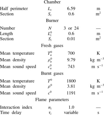
Analytical expressions of the eigenfrequencies (3.13) of azimuthal modes are compared with results obtained with AVSP (Nicoud et al. Reference Nicoud, Benoit, Sensiau and Poinsot2007), a full 3D Helmholtz solver, for two cases:
-
(i) a simplified academic configuration with
$N=3$
burners (§ 5): -
(ii) a realistic case with
$N=24$
burners (§ 6).


4.1. Description of the configurations
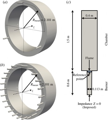
The 3D geometries correspond to BC set-ups with
 $N=3$
or
 $N=24$
burners (figure 8), similar to figure 3 (the physical and geometrical parameters are defined in table 1). The burner/chamber interfaces are placed at
 $z=0$
and the flames are on the burner side. The flame width is equal to 2 mm, which guarantees its compactness with respect to the acoustic wavelength. The boundary conditions correspond to impermeable walls everywhere except at the upstream end of the burners where an impedance
 $Z=0$
(i.e.
 $p^{\prime }=0$
) is imposed to mimic a connection to a large plenum. For the
 $N=3$
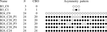
burner configuration, two cases are investigated (table 2): first with identical burners and then with two types of burners with different time delays
 ${\it\tau}_{1}$
and
 ${\it\tau}_{2}$
. The interaction index of the flames is set to the same value
 $n=1.0$
(knowing that typical low-frequency values for
 $n$
are around
 $T^{0}/T_{u}^{0}-1\simeq 1.57$
here (Poinsot & Veynante Reference Poinsot and Veynante2011)) in each burner.
Toy models to validate the ATACAMAC methodology. (a) Perfect annular chamber with
 $N=3$
, (b)
 $N=24$
cylindrical burners, (c) burner/chamber configuration.

The parameters used for numerical applications. They correspond to a typical large-scale industrial gas turbine.

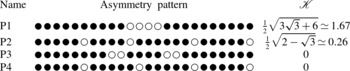
The BC configurations investigated with both the 3D Helmholtz solver AVSP and the analytical approach ATACAMAC. ○: burner without CBO; ●: burner with CBO.

For the
 $N=24$
configuration (figure 8
b), two types of burners with different time delays are mixed to mimic the combustion chamber where burners can be equipped (or not) with CBOs to modify their flame response (Krueger et al.
Reference Krueger, Hueren, Hoffmann, Krebs, Flohr and Bohn2000; Berenbrink & Hoffmann Reference Berenbrink and Hoffmann2001). Table 2 displays the circumferential patterns (● for CBO burners and ○ for burners without CBOs) that are considered.
4.2. Description of the 3D acoustic code
The assumptions and results of ATACAMAC can be validated using a full 3D acoustic solver called AVSP (Selle et al.
Reference Selle, Benoit, Poinsot, Nicoud and Krebs2006; Nicoud et al.
Reference Nicoud, Benoit, Sensiau and Poinsot2007; Sensiau et al.
Reference Sensiau, Nicoud and Poinsot2009; Silva et al.
Reference Silva, Nicoud, Schuller, Durox and Candel2013), which solves the Helmholtz equation in a reactive flow without the assumptions used in ATACAMAC (Nicoud et al.
Reference Nicoud, Benoit, Sensiau and Poinsot2007), but of course at a higher cost. The AVSP solver takes into account the interaction between combustion and acoustics. It solves the eigenvalue problem issued from the discretization on unstructured meshes of the Helmholtz equation at zero Mach number. The meshes contain approximately two million cells (corresponding to the ratio of the wavelength to the longest cell length
 ${\it\lambda}/{\rm\Delta}h_{max}\simeq 250$
), which is sufficient considering the simplicity of the geometry and the wavelength of the first azimuthal mode. Source terms due to flames are modelled using FTFs (Crocco Reference Crocco1951). The local heat-release fluctuations in the burner
 $i$
are expressed as
 $$\begin{eqnarray}q_{i}^{\prime }=n_{u,i}\,\text{e}^{j{\it\omega}{\it\tau}_{i}}\,\boldsymbol{u}^{\prime }(\boldsymbol{x}_{ref,i})\boldsymbol{\cdot }\boldsymbol{n}_{ref,i},\end{eqnarray}$$
where
 $\boldsymbol{x}_{ref,i}$
is a reference point upstream of the flame in burner
 $i$
.
The local interaction index
 $n_{u,i}$
describes the local flame–acoustic interactions. The values of
 $n_{u,i}$
are assumed to be constant in the flame zone
 $i$
(figure 8) and are chosen to recover the global value of the interaction index
 $n_{i}$
corresponding to the infinitely thin flame when integrated over the flame zone
 $i$
(Nicoud et al.
Reference Nicoud, Benoit, Sensiau and Poinsot2007). For the sake of simplicity, they are also assumed to be independent of frequency. These assumptions allow one to use AVSP to check the precision of the analytical techniques developed in ATACAMAC.
In annular configurations with multiple burners, the heat-release fluctuations in burner
 $i$
are assumed to be driven by velocity fluctuations at the reference point
 $\boldsymbol{x}_{\mathit{ref},\mathit{i}}$
. This assumption, called ISAAC (independence sector assumption in annular combustor) in Sensiau et al. (Reference Sensiau, Nicoud and Poinsot2009), was validated by an LES of a full annular combustor (Staffelbach et al.
Reference Staffelbach, Gicquel, Boudier and Poinsot2009) and is used in the present study. In the infinitely thin flame model used in ATACAMAC the reference points are chosen at the flame locations
 $z_{f,i}$
. The normalized abscissa of the flame is set to
 ${\it\alpha}\simeq 0.91$
(Bauerheim et al.
Reference Bauerheim, Parmentier, Salas, Nicoud and Poinsot2014c
). Three-dimensional effects near the burner/chamber junctions can be accounted for (Pierce Reference Pierce1981) using a standard length correction in the low-frequency range for a flanged tube (Silva et al.
Reference Silva, Guillemain, Kergomard, Mallaroni and Norris2009), which is applied at the downstream burner end (
 ${\rm\Delta}L_{i}=0.4\sqrt{4S_{i}/{\rm\pi}}$
). In AVSP, the reference points are placed a few millimetres upstream of the flames (figure 8) due to numerical accuracy issues (Silva et al.
Reference Silva, Nicoud, Schuller, Durox and Candel2013).
5. Symmetry breaking with
$N=3$
burners

Analytical expressions for the frequency of azimuthal modes (3.13) can be obtained for a generic annular BC configuration with
 $N$
burners. First, the symmetric case (figure 9
a) with
 $N=3$
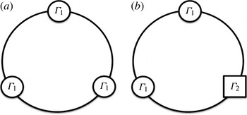
identical burners is studied (§ 5.1). Then, the effect of circumferential variations on combustion instabilities is investigated (§ 5.2) and validated on an asymmetric BC configuration where one type 1 burner is replaced by a type 2 (figure 9
b).
Schematic view of the BC configuration with
 $N=3$
burners for the validation of numerical and analytical resolutions of (2.12); (a) symmetric case (all interaction terms
 ${\rm\Gamma}_{i}$
(2.6) are equal); (b) asymmetric case (two identical burners with the same
 ${\rm\Gamma}_{1}$
and one burner with
 ${\rm\Gamma}_{2}$
).

5.1. Symmetric case with
$N=3$
identical burners

In an axisymmetric configuration where the burners are the same for all sectors (i.e.
 ${\rm\Gamma}_{i}={\rm\Gamma}$
, for all
 $i\in [1,3]$
), only two different mode types exist. Indeed, the splitting strength
 $\mathscr{S}_{0}$
in (3.14) simplifies depending on the mode order
 $p$
and the number of burners
 $N$
(appendix A):
 $$\begin{eqnarray}\left.\begin{array}{@{}l@{}}\text{if }p=3m,\quad \text{for}\ m\in \mathbb{N}\text{ then }\mathscr{S}_{0}=3{\rm\Gamma}^{0},\\ \text{for any other mode of order }p\!:\mathscr{S}_{0}=0.\end{array}\right\}\end{eqnarray}$$
Consequently, only two different classes of modes can develop in annular BC configurations with
 $N=3$
identical burners.
-
(i) Non-degenerate singlets. If
$p=3m,m\in \mathbb{N}$
the splitting strength is not null (
$\mathscr{S}_{0}={\rm\Sigma}_{0}=3{\rm\Gamma}^{0}$
, (3.14)) and the azimuthal mode is split into two components
$V^{-}$
and
$V^{+}$
with different wavenumber perturbations (
${\it\epsilon}^{\pm }$
) and frequencies (
$f^{\pm }$
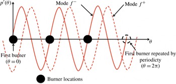
) (3.7): (5.2)Figure 10 displays the mode structure associated with
$$\begin{eqnarray}\left.\begin{array}{@{}c@{}}{\it\epsilon}^{-}=0,\\ {\it\epsilon}^{+}=-3{\rm\Gamma}^{0},\end{array}\right\}\quad \text{corresponding to }\left.\begin{array}{@{}c@{}}f^{-}=\displaystyle \frac{pc^{0}}{2L_{c}},\\ f^{+}=\displaystyle \frac{pc^{0}}{2L_{c}}-\frac{3}{2}\frac{c^{0}{\rm\Gamma}^{0}}{{\rm\pi}L_{c}}.\end{array}\right\}\end{eqnarray}$$
$f^{+}$
and
$f^{-}$
: due to symmetry considerations, these modes (e.g.
$p=3$
) can lock on burners (
$N=3$
) (see Bauerheim et al. (Reference Bauerheim, Cazalens and Poinsot2014a
) for an analytical proof). Their wavelength corresponds to the chamber perimeter (or half of it in the case of a configuration with an even number of burners). The first mode
$V^{-}$
with frequency
$f^{-}$
is standing and imposes a pressure node at every burner; therefore, it is unperturbed by them (
${\it\epsilon}^{-}=0$
); the mode is neutral. The second mode
$V^{+}$
at the frequency
$f^{+}$
is also standing but imposing an azimuthal velocity node (i.e. a pressure anti-node) at every burner (
${\it\epsilon}^{+}=-3{\rm\Gamma}^{0}$
).
-
(ii) Degenerate doublets. All other azimuthal modes (
$p\neq 3m,m\in \mathbb{N}$
) are composed of two eigenmodes
$V^{\pm }$
which have the same frequencies (degenerate modes) because the splitting strength
$\mathscr{S}_{0}=0$
: (5.3)
$$\begin{eqnarray}\left.\begin{array}{@{}c@{}}{\it\epsilon}^{-}=\displaystyle -\frac{3}{2}{\rm\Gamma}^{0},\\ {\it\epsilon}^{+}=\displaystyle -\frac{3}{2}{\rm\Gamma}^{0},\end{array}\right\}\quad \text{corresponding to }\left.\begin{array}{@{}c@{}}f^{-}=\displaystyle \frac{pc^{0}}{2L_{c}}-\frac{3}{4}\frac{c^{0}{\rm\Gamma}^{0}}{{\rm\pi}L_{c}},\\ f^{+}=\displaystyle \frac{pc^{0}}{2L_{c}}-\frac{3}{4}\frac{c^{0}{\rm\Gamma}^{0}}{{\rm\pi}L_{c}}.\end{array}\right\}\end{eqnarray}$$
In this configuration, the transfer matrix of the whole system (
$\unicode[STIX]{x1D648}$
defined in (3.4)) is equivalent to the null matrix. The mode nature is undetermined, as pointed out by Noiray et al. (Reference Noiray, Bothien and Schuermans2011): a standing, spinning or mixed mode can develop. Noiray et al. (Reference Noiray, Bothien and Schuermans2011) have shown that nonlinearities on the FTF can, however, promote one of these natures, a phenomenon that cannot be described by ATACAMAC since it is based on linear FTFs.


The pressure structure of the two components of the azimuthal mode in an
 $N=3$
burner configuration: a standing mode imposing a pressure node at every burner location (—–,
 $f^{-}$
) and a standing mode imposing a pressure anti-node at every burner location (- - -,
 $f^{+}$
).

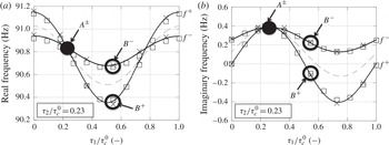
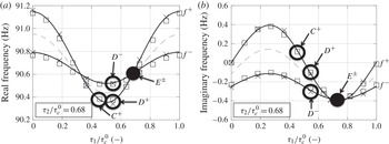
Figures 11 and 12 provide two validation points (marked by ●) of ATACAMAC for symmetric configurations using the full 3D acoustic solver AVSP: modes denoted
 $A^{\pm }$
when
 ${\it\tau}_{1}/{\it\tau}_{c}^{0}={\it\tau}_{2}/{\it\tau}_{c}^{0}=0.23$
and
 $E^{\pm }$
when
 ${\it\tau}_{1}/{\it\tau}_{c}^{0}={\it\tau}_{2}/{\it\tau}_{c}^{0}=0.68$
. Good agreement is obtained between the acoustic code (AVSP) and ATACAMAC.
(a) Real and (b) imaginary parts of the frequencies
 $f^{+}$
and
 $f^{-}$
of the two components of the first mode (
 $p=1$
) in the B3_C1 configuration with the pattern 121 (○ ● ○) and a fixed
 ${\it\tau}_{2}/{\it\tau}_{c}^{0}=0.23$
. —–: ATACAMAC (numerical resolution of (2.12));
 $\Box$
: ATACAMAC (analytical formula (5.6));
 $\times$
: AVSP; - - -: trajectory of the mode average
 $(\,f^{+}+f^{-})/2$
; ●: symmetric case where
 ${\it\tau}_{1}/{\it\tau}_{c}^{0}={\it\tau}_{2}/{\it\tau}_{c}^{0}=0.23$
,
 ${\it\tau}_{c}^{0}$
corresponds to
 $1/f_{0}\simeq 11\ \text{ms}$
.

(a) Real and (b) imaginary parts of the frequencies
 $f^{+}$
and
 $f^{-}$
of the two components of the first mode (
 $p=1$
) in the B3_C1 configuration with the pattern 121 (○ ● ○) and a fixed
 ${\it\tau}_{2}/{\it\tau}_{c}^{0}=68$
. —–: ATACAMAC (numerical resolution of (2.12));
 $\Box$
: ATACAMAC (analytical formula (5.6));
 $\times$
: AVSP; - - -: trajectory of the mode average
 $(\,f^{+}+f^{-})/2$
; ●: symmetric case where
 ${\it\tau}_{1}/{\it\tau}_{c}^{0}={\it\tau}_{2}/{\it\tau}_{c}^{0}=0.68$
,
 ${\it\tau}_{c}^{0}$
corresponds to
 $1/f_{0}\simeq 11\ \text{ms}$
.

5.2. Symmetry breaking with
$N=3$
different burners

This section discusses the behaviour of azimuthal modes when one of the three burners has a different FTF corresponding to a different value of
 ${\rm\Gamma}_{i}^{0}$
(see figure 9
b). In particular, the observation in Perrin & Charnley (Reference Perrin and Charnley1973) and Sensiau et al. (Reference Sensiau, Nicoud and Poinsot2009) will be investigated: circumferential variations with specific patterns obtained by distributing different burner types along the azimuthal direction could split nominally degenerate doublets into non-degenerate singlets, as observed by Sensiau et al. (Reference Sensiau, Nicoud and Poinsot2009). If two burners have a coupling factor
 ${\rm\Gamma}_{1}^{0}$
and the third one
 ${\rm\Gamma}_{2}^{0}$
, (3.13) can be solved with
 $N=3$
and gives the following solution.
-
(i) Non-degenerate singlets. Azimuthal modes with
$p=3m,m\in \mathbb{N}$
are non-degenerate singlets characterized by
$\mathscr{S}_{0}={\rm\Sigma}_{0}=2{\rm\Gamma}_{1}^{0}+{\rm\Gamma}_{2}^{0}$
(3.14) with wavenumber perturbations: (5.4)where
$$\begin{eqnarray}\left.\begin{array}{@{}c@{}}{\it\epsilon}^{-}=0,\\ {\it\epsilon}^{+}=-{\rm\Sigma}_{0}=-2{\rm\Gamma}_{1}^{0}-{\rm\Gamma}_{2}^{0},\end{array}\right\}\quad \text{corresponding to }\left.\begin{array}{@{}c@{}}f^{-}=\displaystyle \frac{pc^{0}}{2L_{c}},\\ f^{+}=\displaystyle \frac{pc^{0}}{2L_{c}}-\frac{c^{0}(2{\rm\Gamma}_{1}^{0}+{\rm\Gamma}_{2}^{0})}{2{\rm\pi}L_{c}},\end{array}\right\}\end{eqnarray}$$
${\rm\Sigma}_{0}=\sum _{i=1}^{N}{\rm\Gamma}_{i}^{0}$
. These modes, as in the symmetric cases, impose a pressure node or pressure anti-node at each burner location leading to two modes with different frequencies:
$f^{+}\neq f^{-}$
.
-
(ii) Nearly degenerate singlets. For other azimuthal modes (
$p\neq 3m,m\in \mathbb{N}$
), (3.13) leads to nearly degenerate singlets (Perrin & Charnley Reference Perrin and Charnley1973): the degenerate doublet encountered in symmetric configurations (denoted DD with
${\it\epsilon}_{DD}=-{\rm\Sigma}_{0}/2=-{\rm\Gamma}_{1}^{0}-{\rm\Gamma}_{2}^{0}/2$
, (5.3)) is split depending on the splitting strength
$\mathscr{S}_{0}={\rm\Gamma}_{1}^{0}-{\rm\Gamma}_{2}^{0}$
(3.14) for the
$N=3$
case with the pattern 121 (○ ● ○, table 2): (5.5)so that
$$\begin{eqnarray}{\it\epsilon}^{\pm }=\underbrace{-{\textstyle \frac{1}{2}}{\rm\Sigma}_{0}}_{{\it\epsilon}_{DD}}\ \pm \underbrace{{\textstyle \frac{1}{2}}\mathscr{S}_{0}}_{\text{Splitting}},\end{eqnarray}$$
(5.6a,b )
$$\begin{eqnarray}{\it\epsilon}^{-}=-{\textstyle \frac{1}{2}}\left({\rm\Gamma}_{1}^{0}+2{\rm\Gamma}_{2}^{0}\right)\quad \text{and}\quad {\it\epsilon}^{+}=-{\textstyle \frac{3}{2}}{\rm\Gamma}_{1}^{0}.\end{eqnarray}$$







These results were validated in figures 11 and 12 for the first azimuthal mode (
 $p=1$
) of the configuration B3_C1 with the pattern 121 (○ ● ○, table 2), where the coupling parameters are defined by (2.8).
When
 $\mathscr{S}_{0}\neq 0$
, the nominally doublet mode is split into two dissimilar azimuthal modes (e.g. modes denoted
 $B^{+}$
and
 $B^{-}$
in figure 11, corresponding to
 ${\it\tau}_{1}/{\it\tau}_{c}^{0}=0.55$
and
 ${\it\tau}_{2}/{\it\tau}_{c}^{0}=0.23$
) with close frequencies and different growth rates, as mentioned in Perrin & Charnley (Reference Perrin and Charnley1973) and Sensiau et al. (Reference Sensiau, Nicoud and Poinsot2009). The term
 $\mathscr{S}_{0}={\rm\Gamma}_{1}^{0}-{\rm\Gamma}_{2}^{0}$
for the pattern 121 (○ ● ○) measures the differences in flame response between the two burner types and controls the degree of degeneracy of the azimuthal mode. It should be noted that some asymmetry could still give degenerate doublets (i.e.
 $\mathscr{S}_{0}=0$
); for instance, the first-order mode (
 $p=1$
) of an
 $N=6$
burner BC configuration with the pattern (● ○ ● ○ ● ○) or (● ● ● ○ ○ ○) is a doublet with
 ${\it\epsilon}=-{\textstyle \frac{3}{2}}({\rm\Gamma}_{1}^{0}+{\rm\Gamma}_{2}^{0})$
.
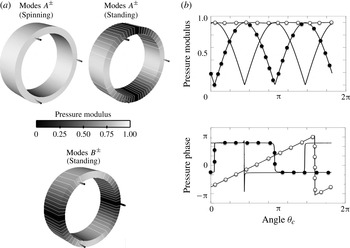
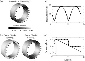
Figure 13 displays the associated mode structure of the symmetric (mode
 $A$
) and asymmetric (mode
 $B$
) cases. For symmetric configurations, the mode structure is undetermined so that both spinning and standing modes can occur (figure 13
a, top). However, breaking the symmetry using two different burner types (e.g. mode
 $B$
with
 ${\it\tau}_{1}/{\it\tau}_{c}^{0}=0.55$
and
 ${\it\tau}_{2}/{\it\tau}_{c}^{0}=0.23$
) leads to standing modes only (figure 13
a, bottom).
Three-dimensional representation and isolines of the pressure modulus (a) and modulus and phase of the acoustic pressure (b) of the first azimuthal modes (
 $p=1$
) of the asymmetric case B3_C1 with the pattern 121 (○ ● ○, table 2) in two situations: mode
 $A$
(
 ${\it\tau}_{1}/{\it\tau}_{c}^{0}={\it\tau}_{2}/{\it\tau}_{c}^{0}=0.23$
) and mode
 $B$
(
 ${\it\tau}_{1}/{\it\tau}_{c}^{0}=0.55$
and
 ${\it\tau}_{2}/{\it\tau}_{c}^{0}=0.23$
). ○:
 $A^{\pm }$
(spinning); ●:
 $A^{\pm }$
(standing); —–:
 $B^{\pm }$
(standing).

5.3. Conclusion on symmetry breaking in the
$N=3$
case

Sections 5.1 and 5.2 show that the splitting strength
 $\mathscr{S}_{0}$
defined by (3.14) controls both the stability and the mode structure of an annular chamber (
 $N=3$
) where two types of burners are installed. Nevertheless, a ‘necessary condition’ for stability can be derived independently of the splitting strength value. Indeed, the imaginary part of the mode average
 $\text{Im}({\it\epsilon}^{+}+{\it\epsilon}^{-})/2$
does not depend on the splitting strength
 $\mathscr{S}_{0}$
but only on the total coupling strength
 ${\rm\Sigma}_{0}=\sum _{i=1}^{N}{\rm\Gamma}_{i}^{0}$
, yielding a necessary condition for stability:
 $$\begin{eqnarray}{\textstyle \frac{1}{2}}\text{Im}({\it\epsilon}^{+}+{\it\epsilon}^{-})=-{\textstyle \frac{1}{2}}\text{Im}({\rm\Sigma}_{0})<0.\end{eqnarray}$$
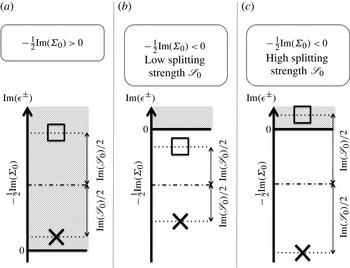
If this condition is not fulfilled (figure 14
a), there is no hope of stabilizing the mode since at least one of the two components of the azimuthal mode (
 $V^{+}$
or
 $V^{-}$
) will remain unstable (e.g.
 $A^{\pm }$
and
 $B^{+}$
in figure 11).
Mode stability for an annular chamber with
 $N$
burners depending on the condition (5.7) and the splitting strength
 $\text{Im}(\mathscr{S}_{0})/2$
.
 $\times$
:
 ${\it\epsilon}^{-}$
;
 $\Box$
:
 ${\it\epsilon}^{+}$
. The splitting strength is
 $\mathscr{S}_{0}^{2}=\sum _{i,j=1}^{N}{\rm\Gamma}_{i}^{0}{\rm\Gamma}_{j}^{0}\cos ((4p{\rm\pi}/N)(j-i))$
(3.14) and measures the difference between the two burner types 1 and 2. Shaded areas correspond to unstable zones. (a) All modes are unstable, (b) all modes are stable and (c) symmetry breaking makes one mode unstable: the splitting strength
 $\mathscr{S}_{0}$
must be reduced to stabilize both modes as in the situation (b).

For a symmetric case where the splitting strength
 $\mathscr{S}_{0}$
is zero, (5.7) is a necessary and sufficient condition to have a stable mode. However, when the symmetry is broken, satisfying condition (5.7) cannot guarantee stability (figure 14
b,c). In this case, the necessary and sufficient condition becomes
 $$\begin{eqnarray}\max (\text{Im}({\it\epsilon}^{+}),\text{Im}({\it\epsilon}^{-}))<0,\end{eqnarray}$$
because the splitting introduced by symmetry breaking (measured by the splitting strength
 $\mathscr{S}_{0}$
) has to be taken into account. For weak splitting (figure 14
b) the two modes
 $V^{+}$
and
 $V^{-}$
remain stable (e.g. eigenmodes
 $D^{\pm }$
in figure 12), but for higher splitting (figure 14
c) one mode can become unstable (e.g. mode
 $C^{+}$
in figure 12). It should be noted that
 $\max (\text{Im}({\it\epsilon}^{+}),\text{Im}({\it\epsilon}^{-}))>\text{Im}({\it\epsilon}^{+}+{\it\epsilon}^{-})/2$
and for a symmetric configuration
 ${\it\epsilon}^{+}={\it\epsilon}^{-}$
.
6. Symmetry breaking in an
$N=24$
burner BC configuration

The conclusions of § 5.3 obtained with
 $N=3$
burners suggest a strategy to stabilize the
 $p$
th mode of a general
 $N$
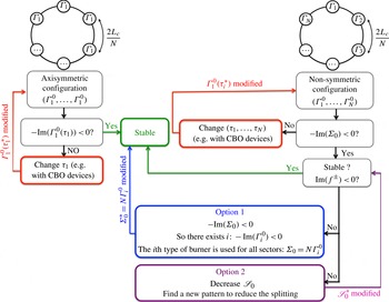
burner configuration, as described in figure 15. Axisymmetric configurations (left part of figure 15) only have one degree of freedom to stabilize the
 $p$
th mode, which is the time delay
 ${\it\tau}_{1}$
: if
 ${\it\tau}_{1}$
is such that condition (5.7) is met, then the configuration is stable.
Strategy to stabilize an annular combustor.

For non-symmetric configurations (right part of figure 15), however, satisfying (5.7) does not guarantee the stabilization of the configuration. In this case, the asymmetry pattern is an additional degree of freedom and two options are available to ensure the stability of the
 $p$
th azimuthal mode.
-
(i) Symmetrize the configuration (option 1). If the condition (5.7) is satisfied, at least one kind of injector satisfies
$-\text{Im}({\rm\Gamma}_{i}^{0})<0$
: this kind of burner can be used for all sectors which leads to stabilization of the mode. This option is the most efficient method to stabilize an azimuthal mode since no splitting occurs. -
(ii) Reduce the asymmetry effect (option 2). Another solution is to keep the same kind of burners (
${\rm\Gamma}_{1}^{0},\dots ,{\rm\Gamma}_{N}^{0}$
) but rearrange them to reduce the splitting of the azimuthal mode and stabilize it. Optimization can be performed to find the best pattern which leads to the smallest value of the splitting strength
$\mathscr{S}_{0}$
.


As an example, symmetry breaking is studied here for an
 $N=24$
burner configuration (Krueger et al.
Reference Krueger, Hueren, Hoffmann, Krebs, Flohr and Bohn2000; Berenbrink & Hoffmann Reference Berenbrink and Hoffmann2001) representative of real industrial gas turbines. First, the stability of the first azimuthal mode (
 $p=1$
) of the symmetric configuration is studied as a function of the time delay
 ${\it\tau}$
(which is the same for all burners), with the interaction index
 $n=1.0$
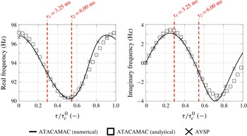
. The results (figure 16) show a very good agreement between the numerical and analytical solutions given by the 3D Helmholtz solver AVSP and ATACAMAC.
Stability map depending on the
 ${\it\tau}$
of the first azimuthal mode (
 $p=1$
) of the symmetric BC configuration with 24 burners. Here,
 ${\it\tau}_{c}^{0}$
is the period of the first azimuthal mode,
 ${\it\tau}_{c}^{0}=1/f^{0}=(2L_{c}/pc^{0})\simeq 11\ \text{ms}$
.

To break the symmetry two different burners are then mixed, characterized by different time delays,
 ${\it\tau}_{1}$
and
 ${\it\tau}_{2}$
(figure 16). A time delay
 ${\it\tau}_{1}=3.25\ \text{ms}$
corresponds approximately to the most unstable burner (
 $\text{Im}(\,f_{AVSP})=2.98\ \text{s}^{-1}$
in figure 16
b), which is assimilated here to the baseline case, a burner without CBO (○ in table 2). Cylindrical burner outlet devices can be mounted on some of the burners (Krueger et al.
Reference Krueger, Hueren, Hoffmann, Krebs, Flohr and Bohn2000; Berenbrink & Hoffmann Reference Berenbrink and Hoffmann2001) to modify the flame time delay and to stabilize the chamber. The length of the cylinder is such that the time lag
 ${\it\tau}_{2}$
from the injection port to the flame front is increased by approximately a quarter of an acoustic period:
 ${\it\tau}_{2}={\it\tau}_{1}+(1/4f^{0})\simeq 6\ \text{ms}$
(since the first azimuthal mode has a frequency
 $f^{0}\simeq 90\ \text{Hz}$
). This corresponds to a stable burner where
 $\text{Im}(\,f_{AVSP})=-1.01\ \text{s}^{-1}$
in figure 16 (● in table 2). It should be noted that the use of 20 burners with
 ${\it\tau}_{2}=6\ \text{ms}$
and four burners with
 ${\it\tau}_{1}=3.25\ \text{ms}$
respects the necessary stability condition given by (5.7) (- - - for the configuration
 $C_{20}$
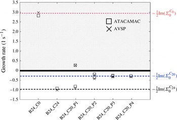
in figure 17). The stability of the four patterns proposed in table 2 is studied using ATACAMAC and AVSP. The results are plotted in figure 17 (growth rates).
Growth rate of the first azimuthal mode (
 $p=1$
) for various asymmetry combinations of burners with and without CBOs: B24_C0 (24 no-CBO burners), B24_C24 (24 CBO burners) and the four patterns B24_C20 (see table 2); - - -: imaginary part of the mode average
 $-\text{Im}({\rm\Sigma}_{0})/2$
depending on the configuration (
 $C_{0}$
,
 $C_{20}$
and
 $C_{24}$
).

-
(i) B24_C0. This configuration corresponds to the unstable baseline case: the necessary condition (5.7) is not satisfied. Some burners have to be changed in order to get a stable combustor.
-
(ii) B24_C20_P1. Twenty CBO devices have been mounted to try to stabilize the mode. The necessary condition (5.7) is satisfied. However, this pattern has a large splitting strength
$\mathscr{S}_{0}$
. Consequently it splits azimuthal modes into two singlets with different growth rates, making the first azimuthal mode unstable. This case is an excellent example of how, for asymmetric circumferential patterns, one can use stable burners that match the condition
$-\text{Im}({\rm\Sigma}_{0})/2<0$
and yet, due to the asymmetry term
$\mathscr{S}_{0}$
, have an unstable mode, as shown in figure 14(c). -
(iii) B24_C20_P2. As suggested by figure 15, a solution to stabilize the mode is to find asymmetry patterns like B24_C20_P2 with a lower splitting strength
$\mathscr{S}_{0}$
for which both singlets remain stable, as shown in figure 14(b). -
(iv) B24_C20_P3 and B24_C20_P4. The pattern B24_C20_P2 induces a low splitting strength and stabilizes the mode. However, optimal asymmetry patterns can be found which lead to no or very low splitting and therefore ensure the mode stabilization. The patterns B24_C20_P3 and B24_C20_P4 give stable degenerate doublets. In these cases,
$\mathscr{S}_{0}=0$
and therefore (5.7) becomes a necessary and sufficient condition for stability. The mode is stable:
$\text{Im}(\,f^{\pm })\simeq -0.25\ \text{s}^{-1}$
. -
(v) B24_C24. As explained in figure 15, the most efficient option to stabilize a mode is to symmetrize the annular combustor with burners that all satisfy the necessary condition (5.7), i.e. 24 burners with a CBO. The mode is very stable:
$\text{Im}(\,f^{\pm })\simeq -1.0\ \text{s}^{-1}$
(figure 17).




Considering the average imaginary part of the modes
 $-\text{Im}({\rm\Sigma}_{0})/2$
(- - - in figure 17), it is interesting to notice that, independently of the asymmetry patterns, combining 20 CBO and four no-CBO burners gives potentially less stable modes than using 24 CBOs: breaking symmetry has a limited interest here compared with adding CBOs to all burners. Nevertheless, if for any reason (ignition, pollution, construction, etc.) one must keep the two types of burner, the present analytical model offers an easy way to optimize the circumferential distribution of the burners by minimizing the imaginary part of the splitting strength
 $\text{Im}(\mathscr{S}_{0})$
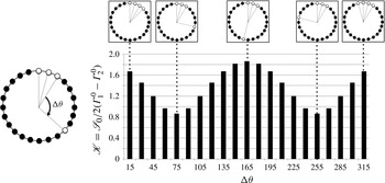
. To illustrate this idea, figure 18 displays the effect of several asymmetry patterns on the splitting strength (
 $\mathscr{S}_{0}$
) using a configuration with 20 CBO–four no-CBO burners. Appendix A shows that the use of two kinds of burners (with coupling parameters
 ${\rm\Gamma}_{1}^{0}$
and
 ${\rm\Gamma}_{2}^{0}$
respectively) yields a splitting strength of the form
 $$\begin{eqnarray}\mathscr{S}_{0}=\hspace{-26.39996pt}\overbrace{2\mathscr{K}}^{\text{Imposed by the pattern}}\hspace{-87.60004pt}\underbrace{({\rm\Gamma}_{1}^{0}-{\rm\Gamma}_{2}^{0})}_{\text{Imposed by the difference between burner types 1 and 2}}\hspace{-62.39996pt},\end{eqnarray}$$
where the reduced splitting strength
 $\mathscr{K}$
depends only on the asymmetry pattern (see table 3 for the analytical expression of
 $\mathscr{K}$
for the four patterns studied). In (6.1),
 ${\rm\Gamma}_{1}^{0}$
and
 ${\rm\Gamma}_{2}^{0}$
are fixed by the burner characteristics so that minimizing
 $\mathscr{S}_{0}$
to increase stability is equivalent to minimizing
 $\mathscr{K}$
.
The reduced splitting strength (
 $\mathscr{K}$
) for several patterns where three no-CBO burners are kept together at the same place and the last no-CBO burner’s place is changed azimuthally. The splitting is then moderately affected by the asymmetry pattern.

Analytical expressions of the reduced splitting strength
 $\mathscr{K}$
for the four patterns described in table 2.

Consequently, an optimization process appears to be a promising approach to find patterns with the minimal value of the reduced splitting strength
 $\mathscr{K}$
. This also highlights the potential of low-order models to perform optimization processes of large problems (here, approximately 1800 patterns are possible at very low cost).
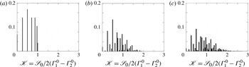
Finally, the enumeration and distributions of the reduced splitting strengths
 $\mathscr{K}$
(obtained numerically using (3.14) and (6.1) for the first azimuthal mode
 $p=1$
) are displayed in figure 19 depending on
 $N_{no\text{-}CBO}$
, the number of no-CBO burner types (
 $N_{no\text{-}CBO}=2,4$
and 6). All possible asymmetry patterns are computed, where
 $N_{no\text{-}CBO}$
burners are chosen as burners without CBOs while the
 $N-N_{no\text{-}CBO}$
other ones correspond to burners with CBOs. The first burner of the pattern is always without a CBO to avoid circular similarities. Figure 19 shows that more numerous and higher reduced splitting strength values are obtained when the number of no-CBO burners (
 $N_{no\text{-}CBO}$
) is increased; these situations are more complex to analyse and optimize. Moreover, only a few patterns lead to a small splitting strength.
Distribution of the reduced splitting strength
 $\mathscr{K}$
versus
 $N_{no\text{-}CBO}$
, the number of burners without CBOs. All possible asymmetry patterns are used to compute each distribution: 23 patterns for
 $N_{no\text{-}CBO}=2$
(a), 2275 for
 $N_{no\text{-}CBO}=4$
(b) and 77 804 for
 $N_{no\text{-}CBO}=6$
(c).

Symmetry breaking can also modify the dynamic nature of the acoustic modes. The modulus and phase of the acoustic pressure of the first azimuthal mode (
 $p=1$
) are plotted in figure 20 for the four studied patterns (table 2), showing two distinct behaviours. It should be noted that only one of the two components of a given azimuthal mode is shown in figure 20.
Effect of the asymmetry pattern on the azimuthal mode nature. Three-dimensional representation and isolines of the pressure modulus (a,c) and modulus and phase of the acoustic pressure over the circumference (b,d). P1 or P3: necessarily standing (●); P3 or P4: any combination of standing (●) or spinning (—–).

-
(i) Patterns P1 and P2. Patterns P1 and P2 give non-degenerate doublets: the two components
$V^{+}$
and
$V^{-}$
of the azimuthal mode are standing (● in figure 20) and oscillate in opposite phase with different (yet very close) frequencies (e.g. 90.3 and 91.3 Hz for the pattern P1). Figure 17 shows that for pattern P1, one mode is amplified whereas the other one is damped, resulting in an unstable standing mode. -
(ii) Patterns P3 and P4. On the other hand, asymmetry patterns leading to degenerate doublets have an undetermined mode structure: the two components
$V^{+}$
and
$V^{-}$
of the azimuthal modes have the same frequencies so that they can be combined to obtain either a spinning (—– in figure 20), a standing (● in figure 20) or a mixed mode.


7. Conclusion
The present work describes a fully analytical approach, completed by a 3D numerical validation, to study the stability of azimuthal thermo-acoustic modes in annular chambers. The analytical model is based on a quasi-one-dimensional zero-Mach-number natural formulation where
 $N$
burners are connected to a downstream annular chamber. Flames are supposed to be compact and are modelled using an FTF, characterized by a coupling factor and a phase shift. Manipulation of the corresponding acoustic equations yields a simple dispersion relation which can be solved analytically in specific situations where the coupling factors are small (weak coupling). This analytical approach allows one to predict the stability of azimuthal modes in symmetric cases where all burners are identical but also to study cases where different burner types are mixed in a chamber, using a predefined pattern. The analytical method highlights the importance of two parameters:
-
(i) a ‘coupling strength’
${\rm\Sigma}_{0}$
, which is the sum of the individual coupling factors
${\rm\Gamma}_{i}^{0}$
of each burner and controls the stability at first order; -
(ii) a ‘splitting strength’
$\mathscr{S}_{0}$
defined in (3.14), which affects the stability and the mode structure and depends on a combination of the coupling parameters of each burner.


First, a symmetric configuration with
 $N$
identical burners with null inlet impedances (i.e.
 $p^{\prime }=0$
) was studied. Only two mode behaviours were observed: degenerate doublets and non-degenerate singlets, the latter being capable of generating warbles (low-frequency oscillations due to a non-degenerate mode (Perrin & Charnley Reference Perrin and Charnley1973)). Then, a non-symmetric case where two different types of burners were distributed in the chamber was studied: symmetry breaking was proved to modify the azimuthal mode behaviour in a simple case with only three burners in an annular chamber. The staging patterns could split nominally degenerate azimuthal modes (doublets) into non-degenerate pairs (singlets), a situation already mentioned in the literature and observed in recent Helmholtz simulations (Sensiau et al.
Reference Sensiau, Nicoud and Poinsot2009).
Finally, the effect of the asymmetry pattern was investigated in an
 $N=24$
burner case representative of industrial gas turbines. Very good agreement was found for all cases between analytical and numerical results, obtained with a 3D Helmholtz solver. The results were compared with experimental observations where CBOs were added to certain burners to control combustion instabilities. A simple criterion was derived to provide a necessary condition to stabilize an annular combustor. Since the asymmetry pattern does not appear in this criterion and the splitting strength is the only control parameter, this shows that symmetry breaking can modify the mode nature but has no real impact on mitigating combustion instabilities in annular chambers. The best method to control a chamber with
 $N=24$
sectors is to use 24 identical burners with FTFs, leading to stable azimuthal modes. However, if keeping only one type of burner is not possible, a strategy to stabilize the mode is proposed: find an optimal pattern that leads to a low splitting of the corresponding azimuthal mode. The general character of this conclusion is limited by the low-coupling assumption, which implies no interaction between burners. (A summary of this method is provided in appendix B; this summary allows the computation of the ‘coupling strength’, the ‘splitting strength’, the frequency and the growth rate of all modes as soon as the FTF of each burner is known.) Strongly coupled situations where burners interfere (Worth & Dawson Reference Worth and Dawson2013b
; Bauerheim et al.
Reference Bauerheim, Parmentier, Salas, Nicoud and Poinsot2014c
) may lead to an effect of the asymmetry pattern on the overall stabilization of the annular engines.
Appendix A. Analytical expression of the splitting strength
The general analytical expression of the splitting strength
 $\mathscr{S}_{0}$
is
 $$\begin{eqnarray}\mathscr{S}_{0}^{2}=\mathop{\sum }\limits_{i,k=1}^{N}{\rm\Gamma}_{i}^{0}{\rm\Gamma}_{k}^{0}\cos \left(\frac{4p{\rm\pi}}{N}[k-i]\right).\end{eqnarray}$$
Using
 $\cos (a-b)=\cos (a)\cos (b)+\sin (a)\sin (b)$
, one may recast the splitting strength as
 $$\begin{eqnarray}\mathscr{S}_{0}^{2}=\left[\mathop{\sum }\limits_{i=1}^{N}{\rm\Gamma}_{i}^{0}\cos (4p{\rm\pi}i/N)\right]^{2}+\left[\mathop{\sum }\limits_{i=1}^{N}{\rm\Gamma}_{i}^{0}\sin (4p{\rm\pi}i/N)\right]^{2}.\end{eqnarray}$$
The above equation can be recast using the identity
 $a^{2}+b^{2}=(a+jb)(a-jb)$
where
 $j^{2}=-1$
:
 $$\begin{eqnarray}\mathscr{S}_{0}^{2}=\left[\mathop{\sum }\limits_{i=1}^{N}{\rm\Gamma}_{i}^{0}\text{e}^{j4p{\rm\pi}i/N}\right]\times \left[\mathop{\sum }\limits_{i=1}^{N}{\rm\Gamma}_{i}^{0}\text{e}^{-j4p{\rm\pi}i/N}\right]={\it\gamma}(-2p)\times {\it\gamma}(2p).\end{eqnarray}$$
Here,
 ${\it\gamma}(k)$
is the
 $k$
th Fourier coefficient of the asymmetry pattern
 ${\rm\Gamma}^{0}$
defined as
 ${\it\gamma}(k)=\sum _{i=1}^{N}{\rm\Gamma}_{i}^{0}\text{e}^{-j2{\rm\pi}ki/N}$
.
Finally, the splitting strength is
 $$\begin{eqnarray}\mathscr{S}_{0}=\sqrt{{\it\gamma}(2p)\times {\it\gamma}(-2p)}.\end{eqnarray}$$
The splitting strength obtained in (A 4) gives some useful results.
-
(i) Noiray et al. (Reference Noiray, Bothien and Schuermans2011) obtained a similar result where the splitting strength is controlled only by
${\it\gamma}_{HR}(2p)$
, the
$2p$
th Fourier coefficient of the heat-release distribution. Equation (A 4) is a generalization of such a result: the network model developed in this paper retains more geometry and flow features than the simple annular rig considered in Noiray et al. (Reference Noiray, Bothien and Schuermans2011). In particular, it is shown here that the mode is controlled by the azimuthal distribution of the coupling parameter (which includes the active flame (
$n$
–
${\it\tau}$
model) but also the geometry characteristics, the upstream impedance
$Z$
of the burners as well as the difference between cold and burnt gases). It appears that all these features can affect the whole asymmetry of the system and therefore the stability and, consequently, cannot be neglected when studying combustion instabilities. -
(ii) If all coupling factors are the same (symmetric configuration), then the spectrum
${\it\gamma}(k)$
is null everywhere except for
$k=0$
or
$k=N$
(where
${\it\gamma}(0)={\it\gamma}(N)={\rm\Sigma}^{0}=\sum _{i=1}^{N}{\rm\Gamma}_{i}^{0}$
is the total coupling of the system), which leads to two types of azimuthal modes.-
(a) If
$p$
is not
$N/2$
,
$N$
,
$3N/2$
etc., then
${\it\gamma}(\pm 2p)=0$
and the splitting strength is null: (A 5)These modes are characterized by no splitting: the two components of the azimuthal mode have the same frequencies and growth rates. They are called ‘degenerate doublets’.
$$\begin{eqnarray}\mathscr{S}_{0}=0.\end{eqnarray}$$
-
(b) However, if
$p=N/2$
,
$N$
,
$3N/2$
etc., then
${\it\gamma}(\pm 2p)=\sum _{i=1}^{N}{\rm\Gamma}_{i}^{0}=N{\rm\Gamma}^{0}$
, which gives (A 6)These modes are characterized by a strong splitting: the two components of the azimuthal mode have different frequencies and growth rates. They are called ‘non-degenerate singlets’.
$$\begin{eqnarray}\mathscr{S}_{0}=N{\rm\Gamma}^{0}.\end{eqnarray}$$
-
-
(iii) If only two types of burner are introduced into the combustion chamber (i.e. coupling factors can only take the value
${\rm\Gamma}_{1}^{0}$
or
${\rm\Gamma}_{2}^{0}$
for
$i\in [1,N]$
), then for a mode satisfying
$p\neq N/2,N,\dots$
, the splitting strength
$\mathscr{S}_{0}$
can be decomposed as (A 7)where the reduced splitting strength
$$\begin{eqnarray}\mathscr{S}_{0}=\hspace{-26.39996pt}\overbrace{2\mathscr{K}}^{\text{Imposed by the pattern}}\hspace{-87.60004pt}\underbrace{({\rm\Gamma}_{1}^{0}-{\rm\Gamma}_{2}^{0})}_{\text{Imposed by the difference between burner types 1 and 2}}\hspace{-62.39996pt},\end{eqnarray}$$
$\mathscr{K}$
depends only on the asymmetry pattern and (
${\rm\Gamma}_{1}^{0}-{\rm\Gamma}_{2}^{0}$
) is fixed by the burner characteristics.








Proof. The Fourier coefficient
 ${\it\gamma}(k)$
can be viewed as a polynomial of degree one with
 $N$
indeterminates (or variables)
 ${\rm\Gamma}_{i}^{0}$
and coefficients depending on the asymmetry pattern. When considering only two burner types (corresponding to coupling factors
 ${\rm\Gamma}_{1}^{0}$
and
 ${\rm\Gamma}_{2}^{0}$
),
 ${\it\gamma}(k)$
reduces to a polynomial of only two variables. The previous point (ii) proves that for modes satisfying
 $p\neq N/2,N,\dots$
, the splitting strength and therefore
 ${\it\gamma}(\pm 2p)$
is null when
 ${\rm\Gamma}_{1}^{0}={\rm\Gamma}_{2}^{0}$
. As
 ${\rm\Gamma}_{1}^{0}-{\rm\Gamma}_{2}^{0}$
is a common root of
 ${\it\gamma}(\pm 2p)$
, which are one-degree polynomials, they can be recast as
 $$\begin{eqnarray}{\it\gamma}(2p)={\it\alpha}_{2p}({\rm\Gamma}_{1}^{0}-{\rm\Gamma}_{2}^{0})\quad \text{and}\quad {\it\gamma}(-2p)={\it\alpha}_{-2p}({\rm\Gamma}_{1}^{0}-{\rm\Gamma}_{2}^{0}),\end{eqnarray}$$
where
 ${\it\alpha}_{2p}$
and
 ${\it\alpha}_{-2p}$
depend only on the asymmetry pattern. Consequently, using (A 4), the splitting strength reads
 $$\begin{eqnarray}\mathscr{S}_{0}=\sqrt{{\it\alpha}_{2p}({\rm\Gamma}_{1}^{0}-{\rm\Gamma}_{2}^{0})\times {\it\alpha}_{N-2p}({\rm\Gamma}_{1}^{0}-{\rm\Gamma}_{2}^{0})}=\underbrace{\sqrt{{\it\alpha}_{2p}{\it\alpha}_{N-2p}}}_{2\mathscr{K}}({\rm\Gamma}_{1}^{0}-{\rm\Gamma}_{2}^{0}).\end{eqnarray}$$
Appendix B. Summary of the analytical method providing the stability map of the
$p$
th azimuthal mode

This appendix summarizes the analytical method to provide the stability map of the
 $p$
th azimuthal mode of a chamber with
 $N$
burners.
-
(i) Compute the coupling factors of each burner:
(B 1)where
$$\begin{eqnarray}{\rm\Gamma}_{i}^{0}=-\frac{j}{2}\frac{S_{i}}{S_{c}}\frac{\mathbb{F}^{0}C_{1-{\it\alpha}}^{k^{0}}[jS_{{\it\alpha}}^{k_{u}^{0}}Z+C_{{\it\alpha}}^{k_{u}^{0}}]+S_{1-{\it\alpha}}^{k^{0}}[jC_{{\it\alpha}}^{k_{u}^{0}}Z-S_{{\it\alpha}}^{k_{u}^{0}}]}{\mathbb{F}^{0}S_{1-{\it\alpha}}^{k^{0}}[jC_{{\it\alpha}}^{k_{u}^{0}}-S_{{\it\alpha}}^{k_{u}^{0}}Z]+C_{1-{\it\alpha}}^{k^{0}}[C_{{\it\alpha}}^{k_{u}^{0}}Z+jS_{{\it\alpha}}^{k_{u}^{0}}]},\end{eqnarray}$$
$\mathbb{F}^{0}=(c^{0}{\it\rho}^{0}/c_{u}^{0}{\it\rho}_{u}^{0})(1+n_{i}\text{e}^{\,j{\it\omega}^{0}{\it\tau}_{i}})$
,
$C_{x}^{y}=\cos (xyL_{i})$
,
$S_{x}^{y}=\sin (xyL_{i})$
,
$k^{0}={\it\omega}^{0}/c^{0}$
,
$k_{u}^{0}={\it\omega}^{0}/c_{u}^{0}$
,
$Z$
is the upstream impedance and
${\it\omega}^{0}=p{\rm\pi}c^{0}/L_{c}$
.
-
(ii) Compute the total ‘coupling strength’
${\rm\Sigma}_{0}=\sum _{i=1}^{N}{\rm\Gamma}_{i}^{0}$
. -
(iii) Compute the ‘splitting strength’
$\mathscr{S}_{0}$
: (B 2)where
$$\begin{eqnarray}\mathscr{S}_{0}=\sqrt{\mathop{\sum }\limits_{i,j=1}^{N}{\rm\Gamma}_{i}^{0}{\rm\Gamma}_{j}^{0}\cos \left(\frac{4p{\rm\pi}}{N}(j-i)\right)}=\sqrt{{\it\gamma}(-2p){\it\gamma}(2p)},\end{eqnarray}$$
${\it\gamma}(k)$
is the
$k$
th Fourier coefficient of the asymmetry pattern.
-
(iv) The
$p$
th azimuthal mode is composed of two modes
$V^{+}$
and
$V^{-}$
with the same order
$p$
but different wavenumber perturbations
${\it\epsilon}^{\pm }$
given by (B 3a,b )
$$\begin{eqnarray}{\it\epsilon}^{+}=-{\textstyle \frac{1}{2}}\left({\rm\Sigma}_{0}+\mathscr{S}_{0}\right)\quad \text{and}\quad {\it\epsilon}^{-}=-{\textstyle \frac{1}{2}}\left({\rm\Sigma}_{0}-\mathscr{S}_{0}\right).\end{eqnarray}$$
-
(v) Then compute the complex frequency of the system from the definition of the wavenumber perturbation (
$k^{\pm }L_{c}=((2{\rm\pi}f^{\pm })/c^{0})L_{c}=p{\rm\pi}+{\it\epsilon}^{\pm }$
) and (B 3): (B 4)
$$\begin{eqnarray}f^{\pm }=\frac{pc^{0}}{2L_{c}}-\frac{c^{0}\left({\rm\Sigma}_{0}\pm \mathscr{S}_{0}\right)}{4{\rm\pi}L_{c}}.\end{eqnarray}$$
-
(vi) Finally, the two components of the
$p$
th azimuthal mode can have different frequencies (
$f^{+}\neq f^{-}$
, non-degenerate singlets) if
$\mathscr{S}_{0}\neq 0$
or the same frequencies (
$f^{+}=f^{-}$
, degenerate doublets) if
$\mathscr{S}_{0}=0$
. The growth rate of each mode is obtained from the imaginary part of the complex frequency obtained in (B 4): (B 5)
$$\begin{eqnarray}\text{Growth rate}^{\pm }=\text{Im}(\,f^{\pm })=-\frac{c^{0}}{4{\rm\pi}L_{c}}\text{Im}({\rm\Sigma}_{0}\pm \mathscr{S}_{0}).\end{eqnarray}$$







Nomenclature
-
${\it\alpha}_{i}$
-
Normalized abscissa of the
$i$
th flame -
${\it\epsilon}$
-
Wavenumber perturbation
-
${\it\gamma}(\pm 2p)$
-
$\pm 2p$
th Fourier coefficient of the FTF distribution
-
${\rm\Gamma}_{i}$
-
Coupling parameter of the
$i$
th burner -
${\it\lambda}$
-
Acoustic wavelength
-
$\mathscr{K}$
-
Reduced splitting strength
-
$\mathscr{S}_{0}$
-
Splitting strength
-
${\it\omega}$
-
Angular frequency
-
${\it\rho}^{0}$
-
Mean density of the hot gas
-
${\it\rho}_{u}^{0}$
-
Mean density of the cold gas
-
${\rm\Sigma}_{0}$
-
Coupling strength
-
${\it\tau}_{i}$
-
FTF time delay of the
$i$
th burner -
${\it\theta}$
-
Azimuthal angle in the annular cavity
-
$c^{0}$
-
Mean sound speed in the hot gas
-
$c_{u}^{0}$
-
Mean sound speed in the cold gas
-
$f$
-
Complex frequency
-
$k={\it\omega}/c^{0}$
-
Wavenumber
-
$L_{c}$
-
Half perimeter of the annular chamber
-
$L_{i}$
-
Length of the
$i$
th burner -
$N$
-
Number of burners
-
$n_{i}$
-
FTF amplitude of the
$i$
th burner -
$p$
-
Azimuthal mode order
-
$p_{i}^{\prime }$
-
Pressure fluctuations in the annular cavity
-
$p_{b,i}^{\prime }$
-
Pressure fluctuations in the
$i$
th burner -
$q^{\pm }=p^{\prime }\pm {\it\rho}^{0}c^{0}u^{\prime }$
-
Acoustic propagating waves
-
$R_{c}$
-
Radius of the annular chamber
-
$\unicode[STIX]{x1D64D}_{i}$
-
Propagation matrix of the
$i$
th annular sector -
$S_{c}$
-
Cross-section of the annular chamber
-
$S_{i}$
-
Section of the
$i$
th burner -
$\unicode[STIX]{x1D64F}_{i}$
-
Interaction matrix
-
$u_{i}^{\prime }$
-
Azimuthal velocity fluctuations in the annular cavity
-
$w_{b,i}^{\prime }$
-
Axial velocity fluctuations in the
$i$
th burner -
$z$
-
Axial coordinate in the burners
-
$Z_{i}$
-
Upstream impedance of the
$i$
th burner -
$Z_{tr}$
-
Translated or equivalent impedance of the burner and flame
-
$\text{ANR}$
-
Annular network reduction
-
$\text{ATACAMAC}$
-
Analytical tool to analyse and control azimuthal modes in annular combustors
-
$\text{FTF}$
-
Flame transfer function