1. Introduction
In a recent paper (Choi Reference Choi2022a
), high-order strongly nonlinear (SNL) asymptotic models were considered for long surface gravity waves travelling on shallow water of constant depth
 $h_0$
assuming that the long wave parameter
 $\beta$
is small, where
 $\beta$
is defined as the ratio of
 $h_0$
to the characteristic wavelength
 $\lambda _0$
or
 $\beta :=h_0/\lambda _0$
. Depending on the choice of the order of approximation, it was shown that asymptotic long wave models for the depth-averaged horizontal velocity or the horizontal velocity at a fixed vertical level inside the fluid layer could be unstable for a range of wavenumbers or ill-posed in the sense that the growth rates of unstable short waves increase with the wavenumber (Matsuno Reference Matsuno2016; Madsen & Fuhrman Reference Madsen and Fuhrman2020). However, when the asymptotic long wave model is written for the bottom velocity, it was found linearly stable to all disturbances at any order of approximation. In addition, as
 $\beta$
is the only small parameter in the expansion, it was shown that the SNL model reasonably well describes the dynamics of relatively large-amplitude waves (Choi Reference Choi2022a
). A similar expansion has also been applied to large-amplitude internal waves in a two-fluid system (Choi Reference Choi2022b
). This work extends the high-order SNL model to a variable bottom.
Wave deformation over variable bottom has been investigated by a number of researchers using various nonlinear long wave models. Kakutani (Reference Kakutani1971) generalised the Korteweg-de Vries (KdV) equation to the case of a variable bottom, and Johnson (Reference Johnson1972) adopted a variable-coefficient KdV equation to study a solitary wave propagating over a shelf. Mei & Le Méhaute (Reference Mei and Le Méhaute1966), Peregrine (Reference Peregrine1967) and Madsen & Mei (Reference Madsen and Mei1969) derived bi-directional weakly nonlinear (WNL) long wave models for a variable bottom that are equivalent to the Boussinesq model for a flat bottom. Dingemans (Reference Dingemans1994) compared some Boussinesq-type models with the laboratory measurements of periodic waves propagating over a submerged bar whose vertical cross-section is trapezoid shaped. Wei et al. (Reference Wei, Kirby, Grilli and Subramanya1995) derived a SNL Boussinesq model, applied to a solitary wave shoaling on slopes, and compared the computed results with those of a boundary element method for the fully nonlinear (FNL) problem developed by Grilli, Skouruo & Svendsen (Reference Grilli, Skouruo and Svendsen1989). Madsen, Bingham & Liu (Reference Madsen, Bingham and Liu2002) presented a new Boussinesq-type model for highly nonlinear and dispersive waves over a variable bottom such that the linear dispersion relation is accurate for
 $kh_0 \leqslant 40$
, where
 $k$
denotes the characteristic wavenumber. Madsen, Fuhrman & Wang (Reference Madsen, Fuhrman and Wang2006) also generalised this model to cover rapidly varying bathymetry. Chazel, Lannes & Marche (Reference Chazel, Lannes and Marche2010) improved the Green–Naghdi (GN) equations (Green & Naghdi Reference Green and Naghdi1976) for the depth-averaged horizontal velocity valid to
 $O(\beta ^2)$
, proposed a new method of computation for it and compared the computed results with the experimental results of Dingemans (Reference Dingemans1994). Lannes & Marche (Reference Lannes and Marche2015) also introduced a new type of GN equation over a varying bottom that has a mathematical structure suitable for numerical computations. Unfortunately, when they are extended to the next order, or to
 $O(\beta ^4)$
, the Boussinesq or GN equations become unstable and are no longer relevant for numerical computations (Matsuno Reference Matsuno2016; Choi Reference Choi2022a
).
In this work, by generalising the high-order SNL models for a flat bottom, we derive those for a variable bottom written in terms of the bottom velocity by expanding systematically the velocity potential at the bottom in
 $\beta ^2$
. In addition to the fact that the use of the bottom velocity stabilises the asymptotic model, the high-order correction improves the linear dispersion relation, as shown in Choi (Reference Choi2022a
, § 2), and, therefore, better describes the generation of relatively shorter waves that are often inaccurately modelled under the leading-order long wave approximation. To test the proposed high-order model for a variable bottom, we solve numerically the first- and second-order SNL models for two examples: (i) cnoidal waves propagating over a time-independent variable bottom, and (ii) the forced generation of solitary waves by a submerged bottom moving steadily with a transcritical speed, for which a succession of solitary waves is known to be generated and propagate ahead of the disturbance (Wu & Wu Reference Wu and Wu1982; Wu Reference Wu1987; Lee, Yates & Wu Reference Lee, Yates and Wu1989; Grimshaw, Maleewong & Asavanant Reference Grimshaw, Maleewong and Asavanant2009). The numerical results of the SNL models are then compared with those of the WNL long wave model and the FNL computation using the boundary integral method developed by Baker, Meiron & Orszag (Reference Baker, Meiron and Orszag1982).
This paper is organised as follows. Based on the formulation for nonlinear long waves using the bottom velocity in § 2, we present a systematic asymptotic expansion for the velocity potential and the vertical velocity in § 3, from which a high-order SNL model for a variable bottom is derived in § 4. The computed results of the proposed SNL model for the two examples mentioned previously are shown and discussed in § 5. Concluding remarks are given in § 6.
2. Basic formulation for nonlinear long waves
For water waves propagating in two horizontal dimensions, the free surface boundary conditions can be written (Zakharov Reference Zakharov1968) as
 \begin{align} \zeta _t = -\boldsymbol{\nabla }\varPhi \boldsymbol{\cdot }\boldsymbol{\nabla }\zeta + \big(1 + |\boldsymbol{\nabla }\zeta |^2\big) W , \quad \varPhi _t = -\frac {1}{2} |\boldsymbol{\nabla }\varPhi |^2 - g \zeta + \frac {1}{2} \big(1 + |\boldsymbol{\nabla }\zeta |^2\big) W^2 , \end{align}
where
 $\zeta (\boldsymbol{x},t)$
is the surface elevation,
 $\varPhi (\boldsymbol{x},t) = \phi (\boldsymbol{x}, z = \zeta , t)$
is the velocity potential evaluated at the free surface,
 $W$
is the vertical velocity evaluated at the free surface defined by
 $W = \phi _z|_{z = \zeta }$
and
 $g$
is the gravitational acceleration. Here
 $\boldsymbol{x} = (x,y)$
, the subscripts
 $t$
and
 $z$
represent partial differentiations with respect to time
 $t$
and the vertical coordinate
 $z$
, respectively, and
 $\boldsymbol{\nabla}$
is the two-dimensional horizontal gradient given by
 $\boldsymbol{\nabla }= (\partial /\partial x, \partial /\partial y)$
.
There are several ways to write (2.1) as a closed system of two evolution equations for two dynamical variables. For example, one can express
 $W$
in terms of
 $\zeta$
and
 $\varPhi$
, as in the high-order spectral formulation (Dommermuth & Yue Reference Dommermuth and Yue1987; West et al. Reference West, Brueckner, Janda, Milder and Milton1987; Craig & Sulem Reference Craig and Sulem1993), and then find a system for
 $\zeta$
and
 $\varPhi$
, as commonly used for deep or intermediate water depth. Alternatively, for shallow water, one can find the expressions for
 $\varPhi$
and
 $W$
in terms of
 $\zeta$
and the bottom potential
 $\phi _b=\phi (\boldsymbol{x}, z = -h, t)$
and write (2.1) as the evolution equations for these two variables (Choi Reference Choi2022a
).
As the first step to close (2.1), the velocity potential
 $\phi (\boldsymbol{x}, z, t)$
and the vertical velocity
 $w(\boldsymbol{x}, z, t) = \partial \phi /\partial z$
are expanded in Taylor series about the variable bottom
 $z = -h(\boldsymbol{x}, t)$
:
 \begin{align} \phi (\boldsymbol{x}, z, t) & = {\sum _{\!j=0}^\infty } \left [ {\frac {(-1)^j (z + h)^{2j}}{(2j)!}} \phi _{2j} + {\frac {(-1)^j (z + h)^{2j+1}}{(2j+1)!}} w_{2j} \right ]\!, \end{align}
 \begin{align} w(\boldsymbol{x}, z, t) & = {\sum _{\!j=0}^\infty } \left [ -{\frac {(-1)^j (z + h)^{2j+1}}{(2j+1)!}} \phi _{2j+2} + {\frac {(-1)^j (z + h)^{2j}}{(2j)!}} w_{2j} \right ]\! . \end{align}
Here
 $\partial ^2 \phi /\partial z^2 = -{\nabla} ^2\phi$
has been used and
 $\phi _{2j}(\boldsymbol{x},t)$
and
 $w_{2j}(\boldsymbol{x},t)$
for
 $j = 0,1,2,{\cdots}$
are defined, respectively, as
 \begin{align} \phi _{2j} (\boldsymbol{x}, t)= \big ( {\nabla} ^{2j} \phi \big )_{z = -h} , \quad w_{2j} (\boldsymbol{x}, t) = \left ( {\nabla} ^{2j} {\frac {\partial \phi }{\partial z}} \right )_{z = -h} . \end{align}
Here we assume that the bottom is a known function in both space and time. In (2.3a
) note that
 $\phi _{2j}$
for
 $j=0$
is the velocity potential at
 $z=-h$
so that
 $\phi _{0} = \phi _b(\boldsymbol{x}, t)$
.
When
 $\phi$
and
 $w$
in (2.2) are evaluated at
 $z = \zeta$
, the expressions for the free surface variable
 $\varPhi (\boldsymbol{x},t)$
and
 $W(\boldsymbol{x},t)$
can be found as
 \begin{align} \varPhi (\boldsymbol{x}, t) & = {\sum _{\!j=0}^{\infty }} {\left [ {\frac {(-1)^j \eta ^{2j}}{(2j)!}} \phi _{2j} + {\frac {(-1)^j \eta ^{2j+1}}{(2j+1)!}} w_{2j} \right ]}, \end{align}
 \begin{align} W(\boldsymbol{x}, t) & = {\sum _{\!j=0}^\infty } {\left [ -{\frac {(-1)^j \eta ^{2j+1}}{(2j+1)!}} \phi _{2j+2} + {\frac {(-1)^j \eta ^{2j}}{(2j)!}} w_{2j} \right ]}, \end{align}
where
 $\eta$
is the local depth defined by
 \begin{equation} \eta (\boldsymbol{x}, t) = h(\boldsymbol{x}, t) + \zeta (\boldsymbol{x}, t). \end{equation}
When the bottom is flat, as shown in Choi (Reference Choi2022a
), (2.2) can be written, after imposing the bottom boundary condition given by
 $w_0 = 0$
and, therefore,
 $w_{2j} = 0$
, as
 \begin{align} \phi (\boldsymbol{x},z,t) = \cos [(z + h) \boldsymbol{\nabla }] \phi _b\ , \quad w(\boldsymbol{x},z,t) = -\sin [(z + h) \boldsymbol{\nabla }] \boldsymbol{\cdot }\boldsymbol{\nabla }\phi _b . \end{align}
Then, by substituting
 $z = \zeta$
into (2.6),
 $\varPhi$
and
 $W$
can be expressed, in terms of
 $\zeta$
and
 $\phi _b$
, as
 \begin{align} \varPhi = \cos (\eta \boldsymbol{\nabla }) \phi _b , \quad W = -\sin (\eta \boldsymbol{\nabla }) \boldsymbol{\cdot }\boldsymbol{\nabla }\phi _b . \end{align}
Substituting (2.7) into (2.1) yields formally a system of nonlinear evolution equations for
 $\zeta$
and
 $\phi _b$
although the cosine and sine functions in (2.7) need to be expanded in infinite series and, then, truncated for numerical evaluations. This has to be modified for a variable bottom and the derivation of the model will be presented in the following section.
3. Derivation of the long wave model for variable bottom
3.1. Bottom boundary condition
For the variable bottom located at
 $z = -h(x,t)$
, the boundary condition given by
 \begin{equation} -(h_t + \boldsymbol{\nabla }\phi \boldsymbol{\cdot }\boldsymbol{\nabla }h) = {\frac {\partial \phi }{\partial z}} \quad \mbox{at } z = -h(x,t) \end{equation}
can be rewritten, in terms of bottom variables
 $\phi _b$
and
 $w_0$
defined in (2.3), as
 \begin{equation} w_0 = -{\frac {\dot {h}}{1 + |\boldsymbol{\nabla }h|^2}} , \end{equation}
where
 $\dot {h}$
is defined as
 \begin{equation} \dot {h} = h_t + \boldsymbol{\nabla }\phi _b \boldsymbol{\cdot }\boldsymbol{\nabla }h . \end{equation}
As mentioned previously, to write the system given by (2.1) as the evolution equations for
 $\zeta$
and
 $\phi _b$
, one needs to find the expressions for
 $\varPhi$
and
 $W$
in terms of these two variables. This can be achieved using (2.4) once
 $\phi _{2j}$
and
 $w_{2j}$
are expressed in terms of
 $\zeta$
and
 $\phi _b$
, as described subsequently.
First, using the chain rule for differentiation,
 $\phi _2$
and
 $w_2$
can be expressed as
 \begin{align} \phi _2 = \big ( {\nabla} ^2 \phi \big )_{z = -h} & = {\frac {1}{1 + |\boldsymbol{\nabla }h|^2}}\! \left ( {\nabla} ^2 \phi _0 + 2 \boldsymbol{\nabla }w_0 \boldsymbol{\cdot }\boldsymbol{\nabla }h + w_0 {\nabla} ^2 h \right )\!, \end{align}
 \begin{align} w_2 = \big ( {\nabla} ^2 w \big )_{z = -h} & = {\frac {1}{1 + |\boldsymbol{\nabla }h|^2}}\! \left ( {\nabla} ^2 w_0 - 2 \boldsymbol{\nabla }\phi _2 \boldsymbol{\cdot }\boldsymbol{\nabla }h - \phi _2 {\nabla} ^2 h \right )\!. \end{align}
Once the bottom boundary condition given by (3.2) is used for
 $w_0$
, one has the expressions for
 $\phi _2$
and
 $w_2$
in terms of
 $\phi _0$
. The general expressions for
 $\phi _{2j}$
and
 $w_{2j}$
(
 $j = 1,2,{\cdots}$
) can be found recursively as
 \begin{align} \phi _{2j} = \big ( {\nabla} ^{2j} \phi \big )_{z = -h} & = {\frac {1}{1 + |\boldsymbol{\nabla }h|^2}}\! \left ( {\nabla} ^2 \phi _{2j-2} + 2 \boldsymbol{\nabla }w_{2j-2} \boldsymbol{\cdot }\boldsymbol{\nabla }h + w_{2j-2} {\nabla} ^2 h \right )\!,\end{align}
 \begin{align} w_{2j} = \big ( {\nabla} ^{2j} w \big )_{z = -h} & = {\frac {1}{1 + |\boldsymbol{\nabla }h|^2}}\! \left ( {\nabla} ^2 w_{2j-2} - 2 \boldsymbol{\nabla }\phi _{2j} \boldsymbol{\cdot }\boldsymbol{\nabla }h - \phi _{2j} {\nabla} ^2 h \right )\!. \end{align}
Then, substituting (3.4) and (3.5) into (2.4) and the resulting expressions for
 $\varPhi$
and
 $W$
into (2.1), one can find the closed system for the evolution equations for
 $\zeta (\boldsymbol{x},t)$
and
 $\phi _b(\boldsymbol{x},t)$
. The resulting system (2.1) written in infinite series is exact, but needs to be truncated for practical applications. To find a long wave model that is asymptotically consistent, we need to expand
 $\phi _{2j}$
and
 $w_{2j}$
in
 $\beta ^2$
, where
 $\beta = h_0/\lambda _0$
is the long wave parameter defined in § 1.
3.2. Systematic asymptotic expansion
We assume that
 $\phi _{2j}$
and
 $w_{2j}$
(
 $j \geqslant 0$
) in (3.5) can be expanded as
 \begin{align} \phi _{2j} = {\sum _{m=0}^\infty } \phi _{2j, 2m} , \quad w_{2j} = {\sum _{m=0}^\infty } w_{2j, 2m} . \end{align}
In (3.6),
 $\phi _{0, 2m}$
is given by
 \begin{align} \phi _{0, 0} = \phi _b , \quad \phi _{0, 2m} = 0 \quad \mbox{for} \quad m \geqslant 1 , \end{align}
while
 $w_{0, 2m}$
are given, from (3.2), by
 \begin{align} w_{0, 2m} = (-1)^{m+1} \, | \boldsymbol{\nabla }h |^{2m} \, \dot {h} \quad \mbox{for} \quad m \geqslant 0 , \end{align}
where we have used the fact that
 \begin{equation} (1 + | \boldsymbol{\nabla }h |^2 )^{-1} = {\sum _{m=0}^\infty } \, (-1)^m \, | \boldsymbol{\nabla }h |^{2m} , \end{equation}
with
 $| \boldsymbol{\nabla }h|^2 = O(\beta ^2)$
. On the other hand, for
 $j \geqslant 1$
,
 $\phi _{2j, 2m}$
and
 $w_{2j, 2m}$
are given, from (3.5), by
 \begin{align} \phi _{2j, 0} & = {\nabla} ^2 \phi _{2j-2, 0}, \end{align}
 \begin{align} \phi _{2j, 2m} & = {\sum _{l=0}^m} (-1)^{l} | \boldsymbol{\nabla }h |^{2l} \, {\nabla} ^2 \phi _{2j-2, 2(m-l)} \nonumber \\ & + {\sum _{l=0}^{m-1}} (-1)^{l} | \boldsymbol{\nabla }h |^{2l} \left ( 2 \boldsymbol{\nabla }w_{2j-2, 2(m-l-1)} \boldsymbol{\cdot }\boldsymbol{\nabla }h + w_{2j-2, 2(m-l-1)} {\nabla} ^2 h \right ) \, \, \, \, \mbox{for} \, \, m \geqslant 1 , \end{align}
 \begin{align} w_{2j, 2m} & = {\sum _{l=0}^m} (-1)^{l} | \boldsymbol{\nabla }h |^{2l} \left ( {\nabla} ^2 w_{2j-2, 2(m-l)} - 2 \boldsymbol{\nabla }\phi _{2j, 2(m-l)} \boldsymbol{\cdot }\boldsymbol{\nabla }h - \phi _{2j, 2(m-l)} {\nabla} ^2 h \right ) \nonumber \\ & \quad \mbox{for} \, \, m \geqslant 0. \end{align}
Note that
 $\phi _{2j, 2m}/\phi _b = O(\beta ^{2(j+m)})$
and
 $w_{2j, 2m}/|\boldsymbol{\nabla }\phi _b| = O(\beta ^{2(j+m)+1})$
as
 $|\boldsymbol{\nabla }h|^{2m} = O(\beta ^{2m})$
and
 $|w/\boldsymbol{\nabla }\phi | = O(\beta )$
for long waves. Although no small parameter is explicitly introduced, one can see that
 $\phi _{2j}$
and
 $w_{2j}$
are expanded in
 $\beta ^2$
in (3.6).
3.3.
Expansion for
 $\varPhi$
and
$W$
in terms of
$\zeta$
and
$\phi _b$


After substituting (3.6) with (3.7) and (3.9) into (2.4) and collecting terms at
 $O(\beta ^2)$
,
 $\varPhi$
and
 $W$
can be expanded as
 \begin{align} \varPhi = {\sum _{m=0}^\infty } \varPhi _{2m} , \quad W = {\sum _{m=0}^\infty } W_{2m} , \end{align}
where
 $\varPhi _{2m}$
and
 $W_{2m}$
are given by
 \begin{align} \varPhi _0 & = \phi _b, \end{align}
 \begin{align} \varPhi _{2m} & = {\sum _{n=0}^{m-1}} (-1)^n \left [ -{\frac {\eta ^{2n+2}}{(2n+2)!}} \phi _{2n+2, 2(m-n-1)} + {\frac {\eta ^{2n+1}}{(2n+1)!}} w_{2n, 2(m-n-1)} \right ] \, \, \, \, \mbox{for} \, \, m \geqslant 1 , \end{align}
 \begin{align} W_{2m} & = {\sum _{n=0}^m} (-1)^n \left [ -{\frac {\eta ^{2n+1}}{(2n+1)!}} \phi _{2n+2, 2(m-n)} + {\frac {\eta ^{2n}}{(2n)!}} w_{2n, 2(m-n)} \right ] \, \, \, \, \, \mbox{for} \, \, m \geqslant 0, \end{align}
where
 $\phi _{0, 2m} = 0$
for
 $m \geqslant 1$
has been imposed.
Note that both
 $\varPhi _{2m}$
and
 $W_{2m}$
explicitly depend only on
 $\zeta$
and
 $\phi _b$
. Assuming that
 $\eta \boldsymbol{\nabla }= O(h_0/\lambda _0) = O(\beta ) \ll 1$
with
 $\zeta /h = O(a_0/h_0) = O(\alpha ) = O(1)$
, one can notice that
 $\varPhi _{2m}/\varPhi = O(\beta ^{2m})$
and
 $W_{2m}/|\boldsymbol{\nabla }\varPhi | = O(\beta ^{2m+1})$
for
 $m \geqslant 0$
. Here
 $\alpha$
is the nonlinearity parameter defined by the ratio of the wave amplitude
 $a_0$
to the water depth
 $h_0$
, namely
 $\alpha := a_0/h_0$
, and note that no assumption on the magnitude of
 $\alpha$
is made. Therefore, as long as
 $\beta$
remains small, the amplitude
 $a_0$
can be comparable to
 $h_0$
. Of course, the assumption of
 $\beta \ll 1$
is no longer valid for short waves, for which a high-order correction is necessary.
4. High-order long wave model for the bottom potential
4.1. System of nonlinear evolution equations
By substituting (3.10) into (2.1), the nonlinear evolution equations for
 $\zeta$
and
 $\phi _b$
can be obtained as
 \begin{align} \zeta _t = {\sum _{m=0}^\infty } Q_{2m}(\zeta , \phi _b) , \quad \varPhi _t = {\sum _{m=0}^\infty } R_{2m}(\zeta , \phi _b) , \end{align}
where
 $\varPhi$
is given, in terms of
 $\zeta$
and
 $\phi _b$
, by (3.10a
). In (4.1),
 $Q_{2m}$
(
 $m \geqslant 0$
) are given by
 \begin{align} Q_0 = -\boldsymbol{\nabla }\zeta \boldsymbol{\cdot }\boldsymbol{\nabla }\varPhi _0 + W_0 , \quad Q_{2m} = -\boldsymbol{\nabla }\zeta \boldsymbol{\cdot }\boldsymbol{\nabla }\varPhi _{2m} + W_{2m} + |\boldsymbol{\nabla }\zeta |^2 W_{2(m-1)} \, \, \, \, \mbox{for} \, \, m \geqslant 1 , \end{align}
while
 $R_{2m}$
(
 $m \geqslant 0$
) are given by
 \begin{align} R_0 &= -g \zeta - \frac {1}{2} |\boldsymbol{\nabla }\varPhi _0|^2 , \quad R_2 = -\boldsymbol{\nabla }\varPhi _0 \boldsymbol{\cdot }\boldsymbol{\nabla }\varPhi _2 + \frac {1}{2} {W_0}^2 , \end{align}
 \begin{align} R_{2m} &= -\frac {1}{2} {\sum _{\!j=0}^m} \boldsymbol{\nabla }\varPhi _{2j} \boldsymbol{\cdot }\boldsymbol{\nabla }\varPhi _{2(m-j)} + \frac {1}{2} {\sum _{\!j=0}^{m-1}} W_{2j} W_{2(m-j-1)}\nonumber\\&\quad + \frac {1}{2} |\boldsymbol{\nabla }\zeta |^2 {\sum _{\!j=0}^{m-2}} W_{2j} W_{2(m-j-2)} \, \, \, \, \mbox{for} \, \, m \geqslant 2. \end{align}
Note that both
 $Q_{2m}$
and
 $R_{2m}$
are
 $O(\beta ^{2m})$
as
 $\varPhi _{2m}=O(W_{2m})=O(\beta ^{2m})$
.
Similarly to the case of a flat bottom, the evolution equation for
 $\zeta$
given by (4.1a
) can be written in terms of the depth-averaged velocity
 $\overline {\boldsymbol{u}}$
defined by
 \begin{equation} \eta \overline {\boldsymbol{u}} = {\int _{-h}^\zeta } \boldsymbol{\nabla }\phi \, \mathrm{d}z , \end{equation}
whose divergence can be shown, after some manipulation using (2.2a ), (2.4) and (3.5), to be
 \begin{equation} \boldsymbol{\nabla }\boldsymbol{\cdot }(\eta \overline {\boldsymbol{u}}) = \boldsymbol{\nabla }\varPhi \boldsymbol{\cdot }\boldsymbol{\nabla }\zeta - (1 + |\boldsymbol{\nabla }\zeta |^2) W - h_t = -{\sum _{m=0}^\infty } Q_{2m} - h_t . \end{equation}
Then, (2.1a ) can be reduced to
 \begin{equation} \zeta _t + \boldsymbol{\nabla }\boldsymbol{\cdot }(\eta \overline {\boldsymbol{u}}) = -h_t , \end{equation}
which implies conservation of mass when
 $h_t = 0$
.
4.2. Truncated systems
For practical applications, the system (4.1) needs to be truncated, after replacing the upper limit of the summation by
 $M$
, to
 \begin{align} \zeta _t = {\sum _{m=0}^M} Q_{2m}(\zeta , \phi _b) , \quad \varPhi _t = {\sum _{m=0}^M} R_{2m}(\zeta , \phi _b) . \end{align}
The truncated system (4.7) is valid to
 $O(\beta ^{2M})$
, which will be hereinafter referred to as the
 $M$
th-order system.
4.2.1. Zeroth-order model
Under the zeroth-order (
 $M = 0$
) approximation, the leading-order terms in (4.7) can be obtained as
 $\zeta _t = Q_0$
and
 $\varPhi _{0t} = R_0$
or
 \begin{align} \zeta _t + \boldsymbol{\nabla }\boldsymbol{\cdot }(\eta \boldsymbol{\nabla }\phi _b) = -h_t , \quad \phi _{b t} + g \zeta + \frac {1}{2} |\boldsymbol{\nabla }\phi _b|^2 = 0 , \end{align}
which is the (non-dispersive) shallow water equations and neglects any terms of
 $O(\beta ^2)$
or smaller.
4.2.2. First-order model
Under the first-order (
 $M=1$
) approximation, the system correct to
 $O(\beta ^2)$
can be found as
 \begin{align} \zeta _t = Q_0 + Q_2 , \quad (\varPhi _0 + \varPhi _2)_t = R_0 + R_2 , \end{align}
which can be written explicitly, for
 $\varPhi _{2m}$
,
 $Q_{2m}$
and
 $R_{2m}$
(
 $m=0,1$
), respectively, as
 \begin{align}&\qquad \zeta _t + \boldsymbol{\nabla }\boldsymbol{\cdot }\left [ \left ( \eta - {\frac {\eta ^3}{3!}} {\nabla} ^2 \right ) \boldsymbol{\nabla }\phi _b - {\frac {\eta ^2}{2}} \boldsymbol{\nabla }\dot {h} - \left ( {\frac {\eta ^2}{2}} {\nabla} ^2 \phi _b + \eta \dot {h} \right ) \boldsymbol{\nabla }h \right ] = -h_t, \end{align}
 \begin{align}& \left [ \left ( 1 - {\frac {\eta ^2}{2!}} {\nabla} ^2 \right ) \phi _b - \eta \dot {h} \right ]_t + g \zeta + {\frac {1}{2}} \boldsymbol{\nabla }\phi _b \boldsymbol{\cdot }\boldsymbol{\nabla }\phi _b = \boldsymbol{\nabla }\boldsymbol{\cdot }\left ( {\frac {\eta ^2}{2!}} {\nabla} ^2\phi _b \boldsymbol{\nabla }\phi _b + \eta \dot {h} \boldsymbol{\nabla }\phi _b \right ) + {\frac {1}{2}} {\dot {h}}^2, \end{align}
which is valid to
 $O(\beta ^2)$
.
When
 $h$
is independent of time
 $t$
so that
 $h_t = 0$
and
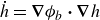 $\dot {h} = \boldsymbol{\nabla }\phi _b \boldsymbol{\cdot }\boldsymbol{\nabla }h$
, this system can be reduced to that derived by Wei et al. (Reference Wei, Kirby, Grilli and Subramanya1995) for the bottom velocity potential.
After taking the horizontal gradient, the first-order system (4.10) can be written, in terms of
 $\boldsymbol{v} = \boldsymbol{\nabla }\phi _b$
, as
 \begin{align}&\qquad\quad \zeta _t + \boldsymbol{\nabla }\boldsymbol{\cdot }\left [ \left ( \eta - {\frac {\eta ^3}{3!}} {\nabla} ^2 \right ) \boldsymbol{v} - {\frac {\eta ^2}{2}} \boldsymbol{\nabla }\dot {h} - \left ( {\frac {\eta ^2}{2}} \boldsymbol{\nabla }\boldsymbol{\cdot }\boldsymbol{v} + \eta \dot {h} \right ) \boldsymbol{\nabla }h \right ] = -h_t ,\end{align}
 \begin{align}& \left [ \boldsymbol{v} - \boldsymbol{\nabla }\left ( {\frac {\eta ^2}{2!}} \boldsymbol{\nabla }\boldsymbol{\cdot }\boldsymbol{v} + \eta \dot {h} \right )\! \right ]_t + \boldsymbol{\nabla }\left ( g \zeta + {\frac {1}{2}} \boldsymbol{v} \boldsymbol{\cdot }\boldsymbol{v} \right ) = \boldsymbol{\nabla }\left [ \boldsymbol{\nabla }\boldsymbol{\cdot }\left \{ {\frac {\eta ^2}{2!}} (\boldsymbol{\nabla }\boldsymbol{\cdot }\boldsymbol{v}) \boldsymbol{v} + \eta \dot {h} \boldsymbol{v} \right \} + {\frac {1}{2}} {\dot {h}}^2 \right ]\!, \end{align}
where
 $\dot {h} = h_t + \boldsymbol{v} \boldsymbol{\cdot }\boldsymbol{\nabla }h$
and
 $\boldsymbol{v}$
is referred to as the bottom velocity. Note that
 $\boldsymbol{v}$
is a tangential velocity at the bottom when it is divided by
 $(1+|\boldsymbol{\nabla }h|^2)^{1/2}$
.
For WNL waves of
 $\zeta /h = O(\beta ^2)$
, or
 $\alpha = O(\beta ^2)$
, the first-order system given by (4.11) can be further simplified to the following WNL model:
 \begin{align}&\qquad\qquad\qquad\qquad \zeta _t + \boldsymbol{\nabla }\boldsymbol{\cdot }\left [ \eta \boldsymbol{v} - \boldsymbol{\nabla }\left ( {\frac {h^3}{3!}} \boldsymbol{\nabla }\boldsymbol{\cdot }\boldsymbol{v} + {\frac {h^2}{2}} \dot {h} \right ) \right ] = -h_t, \end{align}
 \begin{align}& \left [ \boldsymbol{v} - \boldsymbol{\nabla }\left ( {\frac {h^2}{2!}} \boldsymbol{\nabla }\boldsymbol{\cdot }\boldsymbol{v} + h \dot {h} \right )\! \right ]_t + \boldsymbol{\nabla }\left ( g \zeta + {\frac {1}{2}} \boldsymbol{v} \boldsymbol{\cdot }\boldsymbol{v} \right )= \boldsymbol{\nabla }\left [ \boldsymbol{\nabla }\boldsymbol{\cdot }(h h_t \boldsymbol{v}) + {\frac {1}{2}} h_t (h_t + 2\boldsymbol{v}\boldsymbol{\cdot }\boldsymbol{\nabla }h) \right ]\! . \end{align}
Here we have assumed that
 $|\boldsymbol{\nabla }h| = O(h_t) = O(\beta )$
and have used the fact that
 $\boldsymbol{\nabla }(\boldsymbol{\nabla }\boldsymbol{\cdot }\boldsymbol{v}) = {\nabla} ^2\boldsymbol{v}$
with
 $\boldsymbol{\nabla }\times \boldsymbol{v} = \boldsymbol{\nabla }\times \boldsymbol{\nabla }\phi _b = 0$
.
By comparing (4.11a
) with (4.6), one can see that the depth-averaged velocity can be expressed, in terms of
 $\boldsymbol{v}$
, as
 \begin{equation} \overline {\boldsymbol{u}} = \left ( 1 - {\frac {\eta ^2}{3!}} {\nabla} ^2 \right ) \boldsymbol{v} - {\frac {\eta }{2}} \boldsymbol{\nabla }\dot {h} - \left ( {\frac {\eta }{2}} \boldsymbol{\nabla }\boldsymbol{\cdot }\boldsymbol{v} + \dot {h} \right ) \boldsymbol{\nabla }h + O(\beta ^4) , \end{equation}
which can be inverted, under the same order of approximation, to
 \begin{equation} \boldsymbol{v} = \left ( 1 + {\frac {\eta ^2}{3!}} {\nabla} ^2 \right ) \overline {\boldsymbol{u}} + {\frac {\eta }{2}} \boldsymbol{\nabla }\overline {\dot {h}} + \left ( {\frac {\eta }{2}} \boldsymbol{\nabla }\boldsymbol{\cdot }\overline {\boldsymbol{u}} + \overline {\dot {h}} \right ) \boldsymbol{\nabla }h + O(\beta ^4) , \end{equation}
where
 $\overline {\dot {h}}$
is defined by
 \begin{equation} \overline {\dot {h}} = h_t + \overline {\boldsymbol{u}} \boldsymbol{\cdot }\boldsymbol{\nabla }h . \end{equation}
The same result can be obtained from the definition of
 $\overline {u}$
given by (4.4) with (2.2a
) and (3.10a
), as shown in Appendix B. Then, by substituting (4.14) into (4.11) and neglecting terms higher than
 $O(\beta ^2)$
, one can find the first-order system for the depth-averaged velocity given, in conservative form, by
 \begin{equation} \begin{array}{l} \left [ \overline {\boldsymbol{u}} - {\dfrac {1}{\eta }} \boldsymbol{\nabla }\left ( {\dfrac {\eta ^3}{3}} \boldsymbol{\nabla }\boldsymbol{\cdot }\overline {\boldsymbol{u}} + {\dfrac {\eta ^2}{2}} \overline {\dot {h}} \right ) + \left ( {\dfrac {\eta }{2}} \boldsymbol{\nabla }\boldsymbol{\cdot }\overline {\boldsymbol{u}} + \overline {\dot {h}} \right ) \boldsymbol{\nabla }h \right ]_t + \boldsymbol{\nabla }\left ( g \zeta + {\dfrac {1}{2}} \overline {\boldsymbol{u}} \boldsymbol{\cdot }\overline {\boldsymbol{u}} \right ) \nonumber\\[2pt] \\ \quad = \, \boldsymbol{\nabla }\left [ {\dfrac {1}{2}} \left ( \eta \boldsymbol{\nabla }\boldsymbol{\cdot }\overline {\boldsymbol{u}} + \overline {\dot {h}} \right )^2 + {\dfrac {\overline {\boldsymbol{u}}}{\eta }} \boldsymbol{\cdot }\boldsymbol{\nabla }\left ( {\dfrac {\eta ^3}{3}} \boldsymbol{\nabla }\boldsymbol{\cdot }\overline {\boldsymbol{u}} + {\dfrac {\eta ^2}{2}} \overline {\dot {h}} \right ) - \overline {\boldsymbol{u}} \boldsymbol{\cdot }\left ( {\dfrac {\eta }{2}} \boldsymbol{\nabla }\boldsymbol{\cdot }\overline {\boldsymbol{u}} + \overline {\dot {h}} \right ) \boldsymbol{\nabla }h \right ]\! . \end{array} \end{equation}
Here we have used
 $\boldsymbol{\nabla }(\boldsymbol{\nabla }\boldsymbol{\cdot }\overline {\boldsymbol{u}}) = {\nabla} ^2 \overline {\boldsymbol{u}} + O(\beta ^2)$
from the fact that
 \begin{equation} \boldsymbol{\nabla }\times \overline {\boldsymbol{u}} = -\boldsymbol{\nabla }\eta \times \left ( {\frac {\eta }{3}} {\nabla} ^2\overline {\boldsymbol{u}} + {\frac {1}{2}} \boldsymbol{\nabla }\overline {\dot {h}} \right ) + \boldsymbol{\nabla }h \times \boldsymbol{\nabla }\left ({\frac {\eta }{2}} \boldsymbol{\nabla }\boldsymbol{\cdot }\overline {\boldsymbol{u}} + \overline {\dot {h}}\right ) + O(\beta ^4) = O(\beta ^2) , \end{equation}
which is obtained by taking the curl of (4.14) with
 $\boldsymbol{\nabla }\times \boldsymbol{v} = \boldsymbol{\nabla }\times \boldsymbol{\nabla }\phi _b = 0$
.
Using
 $\boldsymbol{\nabla }(\overline {\boldsymbol{u}}\boldsymbol{\cdot }\overline {\boldsymbol{u}}) = 2\overline {\boldsymbol{u}} \boldsymbol{\cdot }\boldsymbol{\nabla }\overline {\boldsymbol{u}} + 2\overline {\boldsymbol{u}}\times (\boldsymbol{\nabla }\times \overline {\boldsymbol{u}})$
with (4.17), one can rewrite (4.16), after some lengthy manipulation, as
 \begin{equation} \overline {\boldsymbol{u}}_t + \overline {\boldsymbol{u}} \boldsymbol{\cdot }\boldsymbol{\nabla }\overline {\boldsymbol{u}} + g \boldsymbol{\nabla }\zeta = {\frac {1}{\eta }} \boldsymbol{\nabla }\left ( {\frac {\eta ^3}{3}} G + {\frac {\eta ^2}{2}} F \right ) - \left ( {\frac {\eta }{2}} G + F \right ) \boldsymbol{\nabla }h , \end{equation}
where
 $G$
and
 $F$
are defined by
 \begin{align} G = \boldsymbol{\nabla }\boldsymbol{\cdot }\overline {\boldsymbol{u}}_t + \overline {\boldsymbol{u}} \boldsymbol{\cdot }\boldsymbol{\nabla }(\boldsymbol{\nabla }\boldsymbol{\cdot }\overline {\boldsymbol{u}}) - (\boldsymbol{\nabla }\boldsymbol{\cdot }\overline {\boldsymbol{u}})^2 , \quad F = (\partial _t + \overline {\boldsymbol{u}} \boldsymbol{\cdot }\boldsymbol{\nabla }) \overline {\dot {h}} . \end{align}
Equation (4.18) along with (4.6) yields the GN equations for a variable bottom correct to
 $O(\beta ^2)$
.
4.2.3. Second-order model
The second-order (
 $M=2$
) system for
 $\zeta$
and
 $\boldsymbol{v}$
that is correct to
 $O(\beta ^4)$
can be found, from (A3), (A5) and (A6) for
 $\varPhi _{2m}$
,
 $R_{2m}$
and
 $Q_{2m}$
(
 $m=0,1,2$
), respectively, as
 \begin{align} \zeta _t = Q_0 + Q_2 + Q_4 , \quad (\varPhi _0 + \varPhi _2 + \varPhi _4)_t = R_0 + R_2 + R_4 . \end{align}
Alternatively, by taking the gradient of (4.20b
), one can find the system for
 $\zeta$
and
 $\boldsymbol{v}$
as
 \begin{align} & \zeta _t + \boldsymbol{\nabla }\boldsymbol{\cdot }\left [ \left \{ \eta - {\frac {\eta ^3}{3!}} {\nabla} ^2 + {\frac {\eta ^5}{5!}} ({\nabla} ^2)^2 \right \} \boldsymbol{v} - {\frac {\eta ^2}{2!}} \boldsymbol{\nabla }\dot {h} - \left ( {\frac {\eta ^2}{2!}} \boldsymbol{\nabla }\boldsymbol{\cdot }\boldsymbol{v} + \eta \dot {h} \right ) \boldsymbol{\nabla }h \right . \nonumber \\[3pt] & \quad \left . + \, {\frac {\eta ^4}{4!}} \boldsymbol{\nabla }\varOmega + {\frac {\eta ^3}{3!}} \boldsymbol{\nabla }\varPi + {\frac {\eta ^2}{2!}} \boldsymbol{\nabla }\left ( |\boldsymbol{\nabla }h|^2 \dot {h} \right ) + \varPhi _4 \boldsymbol{\nabla }h \right ] = -h_t ,\end{align}
 \begin{align} & \left [ \boldsymbol{v} - \boldsymbol{\nabla }\left ( {\frac {\eta ^2}{2!}} \boldsymbol{\nabla }\boldsymbol{\cdot }\boldsymbol{v} + \eta \dot {h} \right ) + \boldsymbol{\nabla }\varPhi _4 \right ]_t + \boldsymbol{\nabla }\left ( g \zeta + {\frac {1}{2}} \boldsymbol{v} \boldsymbol{\cdot }\boldsymbol{v} \right ) \nonumber \\[3pt] & = \boldsymbol{\nabla }\left [ \boldsymbol{\nabla }\boldsymbol{\cdot }\left \{ {\frac {\eta ^2}{2!}} (\boldsymbol{\nabla }\boldsymbol{\cdot }\boldsymbol{v}) \boldsymbol{v} + \eta \boldsymbol{v} \dot {h} \right \} + {\frac {1}{2}} \dot {h}^2 \right ] \nonumber \\[3pt] & \quad - \boldsymbol{\nabla }\left [ \boldsymbol{v} \boldsymbol{\cdot }\boldsymbol{\nabla }\varPhi _4 + {\frac {1}{2}} \left | \boldsymbol{\nabla }\!\left ( {\frac {\eta ^2}{2!}} \boldsymbol{\nabla }\boldsymbol{\cdot }\boldsymbol{v} + \eta \dot {h} \right ) \right |^2 \!+ W_2 (\eta \boldsymbol{\nabla }\boldsymbol{\cdot }\boldsymbol{v} + \dot {h}) - {\frac {1}{2}} |\boldsymbol{\nabla }\zeta |^2 (\eta \boldsymbol{\nabla }\boldsymbol{\cdot }\boldsymbol{v} + \dot {h})^2 \!\right ]\!, \end{align}
where
 $W_2$
and
 $\varPhi _4$
are given by
 \begin{align} W_2 & = {\frac {\eta ^3}{3!}} \boldsymbol{\nabla }\boldsymbol{\cdot }{\nabla} ^2 \boldsymbol{v} + {\frac {\eta ^2}{2!}} \varOmega + \eta \varPi + |\boldsymbol{\nabla }h|^2 \dot {h}, \end{align}
 \begin{align} \varPhi _4 & = {\frac {\eta ^4}{4!}} {\nabla} ^2 \boldsymbol{\nabla }\boldsymbol{\cdot }\boldsymbol{v} + {\frac {\eta ^3}{3!}} \varOmega + {\frac {\eta ^2}{2!}} \varPi + \eta |\boldsymbol{\nabla }h|^2 \dot {h}, \end{align}
with
 $\varOmega$
and
 $\varPi$
defined by
 \begin{align} \varOmega = {\nabla} ^2 \dot {h} + 2{\nabla} ^2\boldsymbol{v} \boldsymbol{\cdot }\boldsymbol{\nabla }h + (\boldsymbol{\nabla }\boldsymbol{\cdot }\boldsymbol{v}) {\nabla} ^2 h , \quad \varPi = | \boldsymbol{\nabla }h |^2 \boldsymbol{\nabla }\boldsymbol{\cdot }\boldsymbol{v} + 2\boldsymbol{\nabla }\dot {h} \boldsymbol{\cdot }\boldsymbol{\nabla }h + \dot {h} {\nabla} ^2 h. \end{align}
In the absence of variable bottom topography (
 $h_t = |\boldsymbol{\nabla }h| = 0$
), the second-order system (4.21) can be reduced to
 \begin{align}&\qquad\quad \zeta _t + \boldsymbol{\nabla }\boldsymbol{\cdot }\left [ \left \{ \eta - {\frac {\eta ^3}{3!}} {\nabla} ^2 + {\frac {\eta ^5}{5!}} ({\nabla} ^2)^2 \right \} \boldsymbol{v} \right ] = 0, \end{align}
 \begin{align}& \left [ \boldsymbol{v} - \boldsymbol{\nabla }\left ( {\frac {\eta ^2}{2!}} \boldsymbol{\nabla }\boldsymbol{\cdot }\boldsymbol{v} - {\frac {\eta ^4}{4!}} \boldsymbol{\nabla }\boldsymbol{\cdot }{\nabla} ^2 \boldsymbol{v} \right ) \right ]_t + \boldsymbol{\nabla }\left ( g \zeta + {\frac {1}{2}} \boldsymbol{v} \boldsymbol{\cdot }\boldsymbol{v} \right )\nonumber\\&\quad = \boldsymbol{\nabla }\left [ \boldsymbol{\nabla }\boldsymbol{\cdot }\left ( {\frac {\eta ^4}{4!}} \boldsymbol{v} {\nabla} ^2 \boldsymbol{\nabla }\boldsymbol{\cdot }\boldsymbol{v} + {\frac {\eta ^4}{16}} \boldsymbol{\nabla }(\boldsymbol{\nabla }\boldsymbol{\cdot }\boldsymbol{v})^2 \right ) \right ]. \end{align}
Note that the original form on the right-hand side of (4.24b ) in Choi (Reference Choi2022a ) contained an error, which was corrected in Choi (Reference Choi2022c ). When linearised, both (4.11) and (4.24) have the real dispersion relation for any wavenumber and are therefore neutrally stable in the absence of bottom topography.
5. Numerical examples
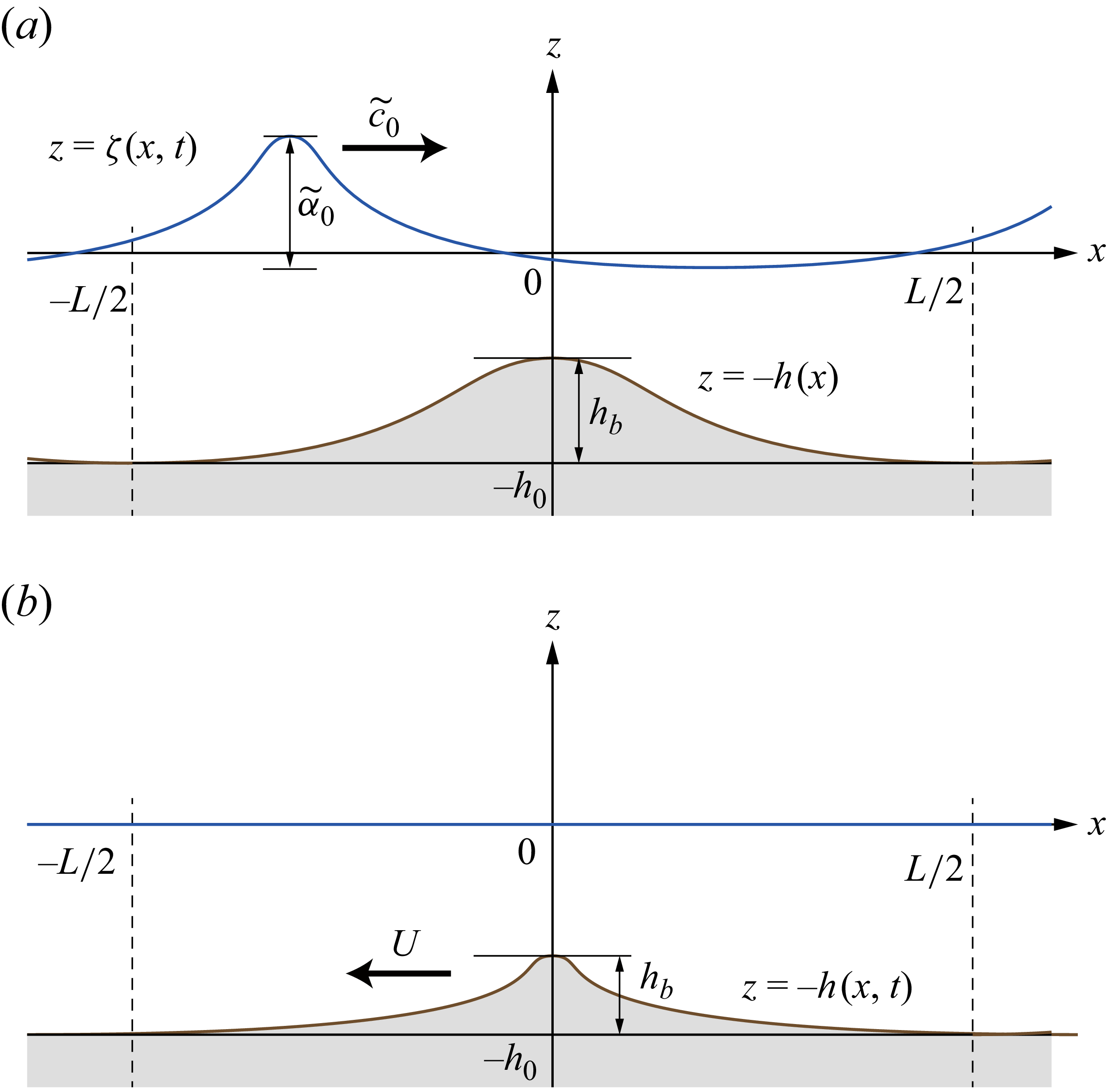
This section shows some computed results for two examples: (i) example : long waves propagating over a time-independent variable bottom
 $z = -h(x)$
; and (ii) example 2: the forced generation of solitary waves by a bottom topography
 $z = -h(x,t)$
moving to the left steadily with a transcritical speed, as shown in figures 1(
 $a$
) and 1(
 $b$
), respectively. The flow is two-dimensional in the vertical cross-section along the propagation direction of waves, and each variable is one-dimensional in space, such as
 $\zeta = \zeta (x,t)$
,
 ${\phi _b}_x = v = v(x,t)$
and
 $h = h(x,t)$
.
Schematic views of initial states for two numerical examples. (
 $a$
) Example 1: long waves propagating over a time-independent variable bottom
 $z = -h(x)$
. (
 $b$
) Example 2: the forced generation of solitary waves by a bottom topography
 $z = -h(x,t)$
moving to the left steadily with a transcritical speed. The blue line
 represents the water surface
 $z = \zeta (x,t)$
and the brown line
 the bottom topography
 $z = -h(x,t)$
.

For numerical computation, each variable is non-dimensionalised with the length scale
 $h_0$
and the time scale
 $\sqrt {h_0/g}$
as
 \begin{equation} (x_\ast , z_\ast , t_\ast , L_\ast , \zeta _\ast , h_\ast , \eta _\ast , v_\ast ) = \left ( {\frac {x}{h_0}}, {\frac {z}{h_0}}, {\frac {t}{\sqrt {h_0/g}}}, {\frac {L}{h_0}}, {\frac {\zeta }{h_0}}, {\frac {h}{h_0}}, {\frac {\eta }{h_0}}, {\frac {v}{\sqrt {g h_0}}} \right )\! . \end{equation}
Henceforth, the asterisks for dimensionless variables will be omitted for brevity. For this one-dimensional system in space, the first-order SNL model (4.11) can be rewritten in dimensionless form as
 \begin{align}&\qquad\quad \zeta _t = \left \{ -(\eta v - {\frac {\eta ^3}{3!}} v_{\textit{xx}}) + {\frac {\eta ^2}{2!}} (\dot {h}_x + v_x h_x) + \eta \dot {h} h_x \right \}_x - h_t, \end{align}
 \begin{align}& \left [ v - \partial _x \left ( {\frac {\eta ^2}{2}} v_x + \eta \dot {h} \right ) \right ]_t = \left \{ -\zeta - {\frac {1}{2}} v^2 + \left ( {\frac {\eta ^2}{2}} v v_x + \eta \dot {h} v \right )_x + {\frac {1}{2}} {\dot {h}}^2 \right \}_x, \end{align}
and the second-order SNL model (4.21) as
 \begin{align}& \zeta _t = \left \{ -( \eta v - {\frac {\eta ^3}{3!}} v_{\textit{xx}} + {\frac {\eta ^5}{5!}} v_{\textit{xxxx}}) + {\frac {\eta ^2}{2!}} (\dot {h}_x + v_x h_x) + \eta \dot {h} h_x \right . \nonumber \\[3pt] & \qquad \left . - \, {\frac {\eta ^4}{4!}} \varOmega _x - {\frac {\eta ^3}{3!}} \varPi _x - {\frac {\eta ^2}{2!}} ( {h_x}^2 \dot {h} )_x - \varPhi _4 h_x \right \}_x - h_t ,\end{align}
 \begin{align}& \left [v - \left ( {\frac {\eta ^2}{2!}} v_x + \eta \dot {h} \right )_x + {\varPhi _4}_x \right ]_t = \left [ -\zeta - {\frac {1}{2}} v^2 + \left ( {\frac {\eta ^2}{2!}} v_x v + \eta v \dot {h} \right )_x + {\frac {1}{2}} \dot {h}^2 \right . \nonumber \\[3pt] & \quad \left . - \, v {\varPhi _4}_x - {\frac {1}{2}} \left \{ \left ( {\frac {\eta ^2}{2!}} v_x + \eta \dot {h} \right )_x \right \}^2 - W_2 (\eta v_x + \dot {h}) + {\frac {1}{2}} {\zeta _x}^2 (\eta v_x + \dot {h})^2 \right ]_x, \end{align}
where
 \begin{align} \left .{\begin{array}{l} \varOmega = \dot {h}_{\textit{xx}} + 2 v_{\textit{xx}} h_x + v_x h_{\textit{xx}}, \quad \varPi = {h_x}^2 v_x + 2 \dot {h}_x h_x + \dot {h} h_{\textit{xx}} \\[5pt] \varPhi _4 = {\dfrac {\eta ^4}{4!}} v_{\textit{xxx}} + {\dfrac {\eta ^3}{3!}} \varOmega + {\dfrac {\eta ^2}{2!}} \varPi + \eta {h_x}^2 \dot {h}, \quad W_2 = {\dfrac {\eta ^3}{3!}} v_{\textit{xxx}} + {\dfrac {\eta ^2}{2!}} \varOmega + \eta \varPi + {h_x}^2 \dot {h}\end{array}} \right \}\!.\end{align}
After assuming the amplitude parameter
 $\alpha \ll 1$
with
 $\alpha =O(\beta ^2)$
,
 $h-h_0=O(\alpha )$
,
 $h_x=O(h_t)=O(\alpha \beta )$
, and neglecting terms higher than
 $O(\alpha \beta ^3,\alpha ^2\beta )$
, the WNL long wave model (4.12) for the one-dimensional system in space becomes
 \begin{align} \zeta _t = \left [ -\eta v + \left ( {\frac {h^3}{3!}} v \right )_{\textit{xx}} \right ]_x - h_t , \quad \left [ v - \left ( {\frac {h^2}{2!}} v \right )_{\textit{xx}} \right ]_t = \left ( -\zeta - {\frac {1}{2}} v^2 \right )_x. \end{align}
After rearranging dispersive terms for
 $h_t = 0$
, it can be shown that (5.4) is the WNL system of Mei & Le Méhaute (Reference Mei and Le Méhaute1966).
Suppose that the flow domain and the bottom topography are periodic in space as
 $\zeta (x,t) = \zeta (x + L,t)$
,
 $v(x,t) = v(x + L,t)$
and
 $h(x,t) = h(x + L,t)$
. We numerically solve the SNL models (5.2) and (5.3) and the WNL model (5.4) in the domain
 $-L/2 \leqslant x \leqslant L/2$
using a pseudo-spectral method with periodic boundary conditions, similarly to the previous work (Choi Reference Choi2022a
, § 6.2) for a flat bottom. The computed results are compared with the FNL computation based on the boundary integral method developed by Baker et al. (Reference Baker, Meiron and Orszag1982), which is summarised in Appendix D.
5.1. The computational method of long wave models
For the spectral approximation of
 $\zeta$
and
 $v$
in the first- and second-order SNL models (5.2) and (5.3) and the WNL model (5.4), the computational domain
 $-L/2 \lt x \lt L/2$
is transformed into
 $-\pi \lt \xi \lt \pi$
, namely
 \begin{equation} -{\frac {L}{2}} \lt x \lt {\frac {L}{2}} \, \, \, \Leftrightarrow \, \, \, -\pi \lt \xi \lt \pi \, \, \, \, \mbox{with} \, \, x = {\frac {L}{2\pi }} \xi \, , \end{equation}
and is divided at equal intervals as
 \begin{equation} x_j = -{\frac {L}{2}} + j \Delta x \, \, \, \Leftrightarrow \, \, \, \xi _j = -\pi + j \Delta \xi \, \, \, \, \mbox{with} \, \, \Delta x = {\frac {L}{N}} , \, \, \Delta \xi = {\frac {2\pi }{N}} \, \, \, \, (j = 0, 1, {\cdots} , N). \end{equation}
Then
 $\zeta$
and
 $v$
at
 $x = x_j = (L/(2\pi )) \xi _j$
can be approximated, respectively, as
 \begin{align} \zeta _j(t) & := \zeta (x_j,t) = {\sum _{k = -\frac {N}{2}}^{\frac {N}{2}-1}} \check {\zeta }_k(t) \mathrm{e}^{{i}k \xi _j} \quad \mbox{with} \quad \check {\zeta }_k(t) \, = {\frac {1}{N}} {\sum _{\!j = 0}^{N-1}} \zeta _j(t) \mathrm{e}^{-{i}k \xi _j}, \end{align}
 \begin{align} v_j(t) & := v(x_j,t) = {\sum _{k = -\frac {N}{2}}^{\frac {N}{2}-1}} \check {v}_k(t) \mathrm{e}^{{i}k \xi _j} \quad \mbox{with} \quad \check {v}_k(t) \, = {\frac {1}{N}} {\sum _{\!j = 0}^{N-1}} v_j(t) \mathrm{e}^{-{i}k \xi _j}. \end{align}
Here the Fourier coefficients
 $\check {\gamma }_k = \check {\zeta }_k$
or
 $\check {v}_k$
are numerically obtained using a fast Fourier transform. In addition, in order to reduce aliasing errors due to approximation of nonlinear terms using the finite Fourier series, the Fourier coefficients
 $\check {\gamma }_k = \check {\zeta }_k$
or
 $\check {v}_k$
are filtered as
 \begin{equation} \check {\gamma }_k = \left \{\!\! \begin{array}{ll} \check {\gamma }_k & \mbox{for} \, |k| \leqslant {\dfrac {N}{2}} - N_{\textit{filter}} , \\[8pt] 0 & \mbox{for} \, |k| \gt {\dfrac {N}{2}} - N_{\textit{filter}} . \end{array} \right . \end{equation}
The evolution equations in (5.2), (5.3) and (5.4) are integrated in time using the fourth-order Runge–Kutta scheme. Then, in order to determine
 $v$
at a new time step, we apply the same iterative scheme as in the previous work (Choi Reference Choi2022a
, (6.14)) to the second equations (5.2b
), (5.3b
) and (5.4b
). For the second-order SNL model, we solve (5.3b
) to obtain
 $\varPsi$
defined by
 \begin{equation} \varPsi \, := \, v - \left ( {\frac {\eta ^2}{2!}} v_x + \eta v h_x \right )_x + \varPhi _{4 x} , \end{equation}
and invert this to find
 $v$
at a new time step using the following iterative scheme:
 \begin{align}& \left ( 1 - {\frac {{\eta _{\textrm{max}}}^2}{2!}} {\frac {\partial ^2}{\partial x^2}} + {\frac {{\eta _{\textrm{max}}}^4}{4!}} {\frac {\partial ^4}{\partial x^4}} \right ) v^{(\mu +1)} = \varPsi ^{(\mu )} + \left \{ \left ( {\frac {\eta ^2}{2!}} - {\frac {{\eta _{\textrm{max}}}^2}{2!}} \right ) v^{(\mu )}_x \right . \nonumber\\& - \left .\left ( {\frac {\eta ^4}{4!}} - {\frac {{\eta _{\textrm{max}}}^4}{4!}} \right ) v^{(\mu )}_{\textit{xxx}} + \eta v^{(\mu )} h_x - {\frac {\eta ^3}{3!}} \varOmega ^{(\mu )} - {\frac {\eta ^2}{2!}} \varPi ^{(\mu )} - \eta v^{(\mu )} {h_x}^3 \right \}_x \quad\!\! (\mu = 0, 1, {\cdots} ) . \end{align}
Here
 $\mu$
denotes the iteration number and
 $\eta _{\textrm{max}} = {\max _{0 \leqslant j \leqslant N}} \eta (x_j,t)$
is a numerical parameter to accelerate the convergence rate (see Choi Reference Choi2022a
, Appendix C). Note that
 $\varPsi$
in (5.9) corresponds to the inside of the bracket on the left-hand side of (5.3b
). The stopping condition of this iteration (5.10) was set using the residual
 $r^{(\mu )}(t)$
as
 \begin{equation} r^{(\mu )}(t) \, := {\max _{0 \leqslant j \leqslant N}} |v^{(\mu )}(x_j,t) - v^{(\mu -1)}(x_j,t)| \, \lt \, 10^{-9} . \end{equation}
In the case of a variable bottom, the convergence rate of this iterative scheme (5.10) depends sensitively on the initial guess
 $v^{(0)}$
. We improve the convergence of (5.10) by adopting a solution of the finite difference approximation of (5.9) as the initial guess
 $v^{(0)}$
(see Appendix C). Similarly, we can obtain
 $v$
at a new time step in (5.2b
) of the first-order SNL model and (5.4b
) of the WNL model.
5.2.
Example 1: long waves propagating over a time-independent variable bottom (
$h_t = 0$
)

The initial state of this example is schematically depicted in figure 1(
 $a$
). The initial wave and the bottom topography are set as follows. First, the initial wave profile
 $z = \zeta (x, t=0)$
is the cnoidal wave solution of the KdV equation given by
 \begin{equation} \zeta (x, t=0) = -\tilde {\alpha }_0 \, B(\ell ) + \tilde {\alpha }_0 \, \mathrm{cn}^2 \left \{ {\frac {\sqrt {3\tilde {\alpha }_0}}{2\ell }} (x - x_0) \, \Big | \, \ell \right \} \! , \end{equation}
with
 \begin{equation} B(\ell ) \, := \, 1 - {\frac {1}{\ell ^2}} + {\frac {1}{\ell ^2}} {\frac {E(\ell )}{K(\ell )}} , \end{equation}
where
 $\ell$
denotes the modulus of the cnoidal function,
 $K(\ell )$
and
 $E(\ell )$
are the complete elliptic integrals of the first and second kind, respectively, and
 $\tilde {\alpha }_0 = H_0/h_0$
is the dimensionless height of the initial wave. The wave crest is located at
 $x = x_0$
. When the wavelength
 $L$
and the wave height
 $\tilde {\alpha }_0$
are given, the modulus
 $\ell$
can be determined by
 \begin{equation} \ell \boldsymbol{\cdot }K(\ell ) = {\frac {\sqrt {3 \tilde {\alpha }_0}}{4}} L . \end{equation}
The phase speed
 $\tilde {c}_0$
of the initial cnoidal wave in (5.12) is given by
 \begin{equation} \tilde {c}_0 = 1 + {\frac {1}{2}} \tilde {\alpha }_0 \left \{ 2 - {\frac {1}{\ell ^2}} - 3 B(\ell ) \right \}\!, \end{equation}
where
 $\tilde {c}_0$
is scaled by
 $\sqrt {g h_0}$
. Next, the time-independent bottom topography
 $z = -h(x)$
is set using the cnoidal function as
 \begin{equation} h(x) = 1 - h_b \, \mathrm{cn}^6 \left \{ {\frac {2}{L}} K(\ell _b) x \, \Big | \, \ell _b \right \}\!, \end{equation}
where
 $h_b$
is the height of the topography, as shown in figure 1(
 $a$
), and the modulus
 $\ell _b$
is related to the nome
 $q_{\ell _b}$
by
 \begin{equation} q_{\ell _b} = \mathrm{exp} \left ( -\pi {\frac {K^{\prime }(\ell _\textit{b})}{K(\ell _\textit{b})}} \right ) \, \, \, \, \, \mbox{with} \, \, K^{\prime }(\ell _b) = K(\ell _b^{\prime }) = K(\sqrt {1 - {\ell _b}^2}) . \end{equation}
Figures 2 and 3 show some computed results of the first- and second-order SNL long wave models (5.2) and (5.3) and the WNL long wave model (5.4) with
 $L = 60$
,
 $x_0 = -20$
in (5.12) and
 $h_b = 0.75$
and
 $q_{\ell _b} = 0.01$
in (5.16). The results are compared with the FNL computation. Figure 2(
 $d$
) shows the shape of the bottom topography
 $z = -h(x)$
. The total number
 $N$
of the spectral approximation in (5.7) and the time increment
 $\Delta t$
of the fourth-order Runge–Kutta scheme for the evolution equations are set to
 $N = 2048$
and
 $\Delta t = 0.05$
, respectively. The threshold
 $N_{\textit{filter}}$
for the de-aliasing filter in (5.8) is set to
 $N_{\textit{filter}} = 900$
for SNL and
 $N_{\textit{filter}} = 400$
for WNL and FNL.
Comparison of the time evolution of the wave profile
 $z = \zeta (x,t)$
of example 1. The wave profiles
 $z = \zeta (x,t)$
at
 $t = 0$
,
 $9$
,
 $18$
,
 $27$
,
 $36$
,
 $45$
and
 $54$
are plotted in each figure. The initial wave profile
 $\zeta (x, t=0)$
is given by (5.12) with
 $L = 60$
and
 $x_0 = -20$
for (
 $a$
)
 $\tilde {\alpha }_0 =0.05$
, (
 $b$
)
 $\tilde {\alpha }_0 =0.07$
and (
 $c$
)
 $\tilde {\alpha }_0 =0.09$
, where
 $\tilde {\alpha }_0 = H_0/h_0$
denotes the dimensionless wave height of the initial wave. The red line
 represents the first-order SNL long wave model, the blue line
 the second-order SNL model, the green line
 the WNL long wave model and the black dashed line
 the FNL computation. The brown line
 in (
 $d$
) shows the shape of the bottom topography
 $h(x)$
given by (5.16) with
 $h_b = 0.75$
and
 $q_{\ell _b} = 0.01$
. The time increment
 $\Delta t$
of the fourth-order Runge–Kutta scheme, the total number
 $N$
of the spectral approximation in (5.7) and the threshold
 $N_{\textit{filter}}$
for the de-aliasing filter in (5.8) are set to
 $\Delta t = 0.05$
,
 $N = 2048$
and
 $N_{\textit{filter}} = 900$
(SNL) and
 $400$
(WNL and FNL), respectively. Panels (b i) and (b ii) enlarge (
 $b$
) at
 $t = 45$
and
 $54$
, respectively. Panels (c i) and (c ii) enlarge (
 $c$
) at
 $t = 45$
and
 $54$
, respectively.

Three-dimensional plot for the time evolution of the wave profile
 $z = \zeta (x,t)$
of example 1 for
 $\tilde {\alpha }_0 = 0.09$
in the
 $(x,t,z)$
space. The time interval is 0.5. For further information, see the caption of figure 2. (
 $a$
) First-order SNL, (
 $b$
) second-order SNL, (
 $c$
) WNL, (
 $d$
) FNL.

Figures 2(
 $a$
), 2(
 $b$
) and 2(
 $c$
) show the computed results of time evolution of the wave profile
 $z = \zeta (x,t)$
for
 $\tilde {\alpha }_0 = 0.05$
,
 $0.07$
and
 $0.09$
, respectively, where
 $\tilde {\alpha }_0 = H_0/h_0$
denotes the wave height of the initial cnoidal wave (5.12). Figures 2(b i) and 2(b ii) enlarge (
 $b$
) at
 $t = 45$
and
 $54$
, respectively, and figures 2(c i) and 2(c ii) enlarge (
 $c$
) at
 $t = 45$
and
 $54$
, respectively. Figures 3(
 $a$
), 3(
 $b$
), 3(
 $c$
) and 3(
 $d$
) compare the three-dimensional plots in the
 $(x,t,z)$
space of time evolution of the wave profile
 $z = \zeta (x,t)$
for
 $\tilde {\alpha }_0 = 0.09$
using the first- and second-order SNL, WNL and FNL models, respectively. The wave height increases as the wave approaches the hump of the bottom, and the long cnoidal wave disintegrates into several shorter waves or rank-ordered solitary waves after travelling over the top of the hump at
 $x = 0$
. Compared with the FNL computation, it is found that the second-order SNL model produces more accurate solutions in this range of the height
 $\tilde {\alpha }_0$
than the first-order SNL and WNL models, which fail to capture the disintegration process correctly. It should be noted that the shorter waves generated by the first-order SNL model propagate faster than those of the second-order SNL model or the FNL solutions. This seems to be related to the linear dispersion relation of the SNL models. The full linear dispersion relation for small-amplitude sinusoidal waves with the wavenumber
 $k$
and the wave frequency
 $\omega$
propagating on water of constant depth
 $h_0$
is given by
 \begin{equation} \omega ^2 = g k \tanh kh_0 \quad \mbox{or} \quad {\frac {c^2}{gh_0}} = {\frac {\tanh kh_0}{kh_0}} \quad \mbox{with} \quad c = {\frac {\omega }{k}} . \end{equation}
For long waves with
 $kh_0 \ll 1$
, this dispersion relation is approximated by the
 $M$
th order SNL model as (Choi Reference Choi2022a
, (2.16))
 \begin{equation} \omega ^2 = gh_0 k^2 \boldsymbol{\cdot }{\dfrac {1 + {\sum _{m=1}^M} {\dfrac {(kh_0)^{2m}}{(2m+1)!}}} {1 + {\sum _{m=1}^M} {\dfrac {(kh_0)^{2m}}{(2m)!}}}} \quad \mbox{or} \quad {\dfrac {c^2}{gh_0}} = {\dfrac {1 + {\sum _{m=1}^M} {\dfrac {(kh_0)^{2m}}{(2m+1)!}}} {1 + {\sum _{m=1}^M} {\dfrac {(kh_0)^{2m}}{(2m)!}}}} . \end{equation}
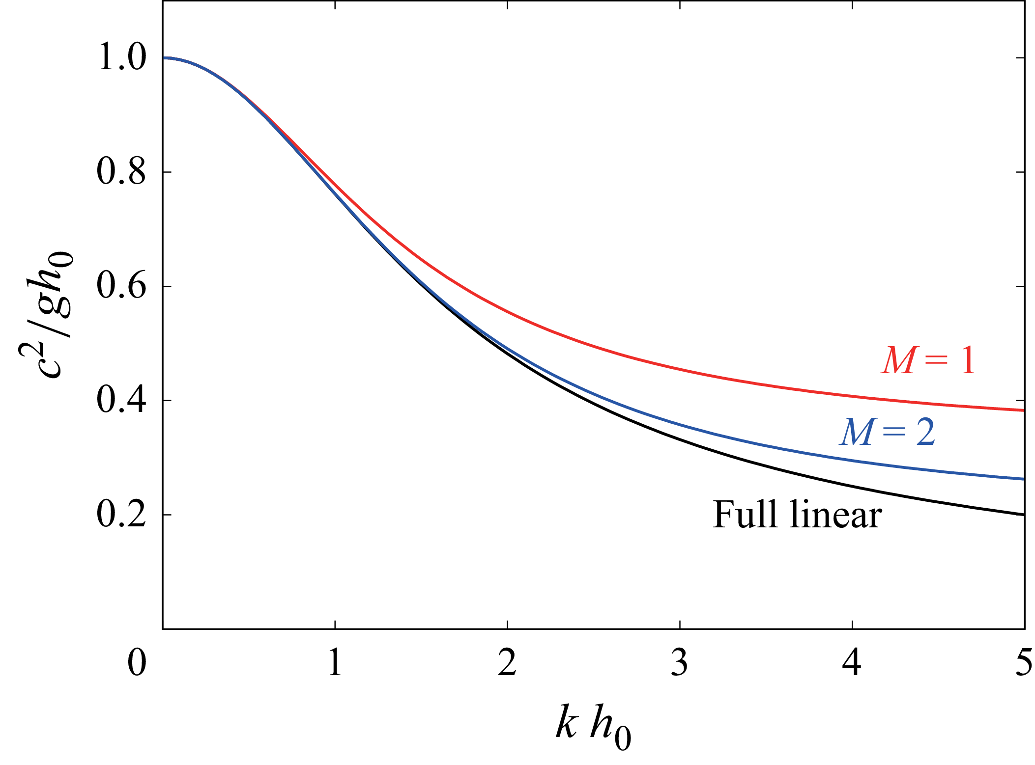
Figure 4 compares the variation of
 $c^2/(gh_0)$
with the dispersion parameter
 $kh_0$
in (5.18) and (5.19) with
 $M=1$
and
 $2$
. We can see that the linear wave speed for the second-order SNL model (
 $M=2$
) agrees with that of the Euler equations for
 $k h_0 \lt 2$
, while the agreement for the first-order SNL model (
 $M=1$
) is observed for
 $k h_0 \lt 1$
. The wave speed for the first-order model is always greater than that of the second-order or FNL model, as observed in our numerical results. Therefore, one can conclude that the short-wavelength behaviour is captured better by increasing the order of approximation.
Variation of the wave speed squared
 $c^2/g h_0$
with the dispersion parameter
 $k h_0$
in the linear dispersion relations. The black line
 represents the full linear dispersion relation (5.18). The red line
 and blue line
 denote the linear dispersion relation (5.19) with
 $M = 1$
(first-order SNL) and
 $M = 2$
(second-order SNL), respectively.

Figure 5 shows the variation of the shoaling rate
 $\| \zeta /h \|_{\textrm{max}}$
for
 $15 \leqslant t \leqslant 20$
when the crests of incident waves (
 $\tilde {\alpha }_0 = 0.09$
,
 $0.11$
,
 $0.13$
,
 $0.15$
and
 $0.17$
) are on the up-slope, where
 \begin{equation} \left \| \, {\frac {\zeta }{h}} \, \right \|_{\textrm{max}} \, := \, {\max _{-L/2 \,\leqslant\, x \,\leqslant\, L/2}} \left | {\frac {\zeta (x,t)}{h(x)}} \right | . \end{equation}
Variation of the shoaling rate
 $\| \zeta /h \|_{\textrm{max}}$
on the up-slope with time
 $t$
(example 1). Each numeral in the figure shows the value of the height
 $\tilde {\alpha }_0 = H_0/h_0$
of the initial wave (5.12). The shoaling rate
 $\| \zeta /h \|_{\textrm{max}}$
is defined by (5.20). The red line
 represents the first-order SNL long wave model, the blue line
 the second-order SNL model, the green line
 the WNL long wave model and the black dashed line
 the FNL computation. For further information, see the caption of figure 2.

The results show that, for the bottom topography given by (5.16), the second-order SNL model better approximates the shoaling rate
 $\| \zeta /h \|_{\textrm{max}}$
of the FNL solution for
 $\| \zeta /h \|_{\textrm{max}} \lt 0.8$
than the first-order SNL and WNL models.
5.3. Example 2: forced generation of solitary waves by a bottom topography moving steadily with a transcritical speed
As mentioned in § 1, a submerged hump moving steadily with a transcritical speed in a layer of shallow water, as shown in figure 1(
 $b$
), can generate a succession of solitary waves propagating ahead of the hump. In this example, we perform numerical computation for this phenomenon, namely the forced generation of solitary waves by a bottom topography moving to the negative
 $x$
direction with constant speed
 $U$
in water of finite depth
 $h_0$
, using the proposed SNL models. The bottom topography
 $z = -h(x,t)$
in the non-dimensional form is given by
 \begin{equation} h(x,t) = 1 - h_b \, \mathrm{ sech}^2 k_b X \, \, \, \, \mbox{with} \, \, X = x + F_r t, \end{equation}
where the Froude number
 $F_r$
is defined by
 \begin{equation} F_r = U/\sqrt {g h_0} . \end{equation}
Then it is convenient to consider this problem in the
 $(X, t)$
frame of reference moving with the bottom topography, instead of the
 $(x, t)$
frame, where
 $X = x + F_r t$
. The Froude number
 $F_r$
and
 $k_b$
in (5.21) are fixed to
 $F_r = 1.01$
and
 $k_b = 0.5$
, respectively. The
 $X$
domain for computation is set to
 $-250 \leqslant X \leqslant 250$
(
 $L = 500$
) and other parameters are
 $N = 2048$
and
 $\Delta t = 0.05$
.
Figures 6(
 $a$
), 6(
 $b$
) and 6(
 $c$
) show the computed results of the wave profiles
 $z = \zeta (X,t)$
at
 $t = 150$
for
 $h_b = 0.05$
,
 $0.075$
and
 $0.1$
, respectively, where
 $h_b$
denotes the height of the bottom topography in (5.21). The shape of the bottom topography is shown in figure 6(
 $d$
). Figures 7(
 $a$
), 7(
 $b$
), 7(
 $c$
) and 7(
 $d$
) compare the three-dimensional plots in the
 $(X,t,z)$
space of time evolution of the wave profile
 $z = \zeta (X,t)$
for
 $h_b = 0.1$
using the first- and second-order SNL, WNL and FNL models, respectively. All three long wave models predicts the generation of solitary waves propagating ahead of the hump, but, when compared with the FNL computations, the second-order SNL model produces the most accurate results.
Comparison of the wave profile
 $z = \zeta (X,t)$
at
 $t = 150$
for example 2. Here
 $X = x + F_r t$
. The height
 $h_b$
of the bottom topography
 $z = -h(x,t) = -h(X)$
in (5.21) is set as (
 $a$
) 0.05, (
 $b$
) 0.075 and (
 $c$
) 0.1. The Froude number
 $F_r$
and
 $k_b$
in (5.21) are fixed to
 $F_r = 1.01$
and
 $k_b = 0.5$
, respectively. The red line
 represents the first-order SNL long wave model, the blue line
 the second-order SNL model, the green line
 the WNL long wave model and the black dashed line
 the FNL. The brown line
 in (
 $d$
) shows the shape of the bottom topography moving to the left. Here
 $L = 500$
,
 $\Delta t = 0.05$
and
 $N = 2048$
with
 $N_{\textit{filter}} = 500$
(SNL),
 $320$
(WNL) and
 $400$
(FNL).

Three-dimensional plot of the time evolution of the wave profile
 $z = \zeta (X,t)$
for
 $F_r = 1.01$
and
 $h_b = 0.1$
in the
 $(X,t,z)$
space of example 2. Here
 $X = x + F_r t$
. The time interval is 2.0. For further information, see the caption of figure 6. (
 $a$
) First-order SNL, (
 $b$
) second-order SNL, (
 $c$
) WNL, (
 $d$
) FNL.

Table 1 summarises the CPU time of each model for example 1 (
 $\tilde {\alpha }_0 = 0.09$
) and example 2 (
 $h_b = 0.1$
) for the computations using a MacBook Pro with an Apple M4 Pro. Note that the CPU time for each long wave model (SNL and WNL) is less than 1/10 of that for the FNL model and no significant increase of the CPU time is observed for the second-order model compared with the first-order model.
Comparison of CPU time to solve each model. Numerical computations were performed using a MacBook Pro with an Apple M4 Pro. The unit of CPU time is seconds. Here SNL (1st) and SNL (2nd) denote the first- and second-order SNL long wave models, respectively. See captions of figures 2 and 6 for details of numerical computations.

From these two numerical examples, one can conclude that the high-order terms in the SNL models should be included to better describe the evolution of nonlinear long waves in the presence of a variable bottom.
6. Conclusions
We have developed the SNL long wave model for a variable bottom with generalising the model proposed by Choi (Reference Choi2022a
) for a flat bottom. Under the assumption that
 $\beta =h_0/\lambda _0\ll 1$
and
 $|\boldsymbol{\nabla }h|=O(\beta )$
, by expanding the velocity potential
 $\phi$
and the vertical velocity
 $w$
at the bottom
 $z = -h(\boldsymbol{x},t)$
, we have presented a system of nonlinear evolution equations (4.1) for the surface elevation
 $\zeta$
and the bottom velocity
 $\boldsymbol{v} = \boldsymbol{\nabla }\phi _b$
that is valid at any order of approximation in
 $\beta ^2$
.
In order to examine their performance with a variable bottom, the first- and second-order SNL models given by (5.2) and (5.3), respectively, are solved numerically using a pseudo-spectral method for the deformation and generation of long waves over a bottom topography. When compared with the FNL computations using the boundary integral method in Appendix D, the computed results in §§ 5.2 and 5.3 have shown that the second-order SNL model produces more accurate results than the first-order SNL model and the WNL model. This demonstrates the importance of high-order (both linear and nonlinear) dispersive effects that cannot be stably described by many of the widely used long wave models for the depth-averaged velocity or the velocity at a fixed vertical level due to the instability or the ill-posedness caused by truncation of the linear dispersion relation for water waves. Therefore, it can be concluded that the high-order SNL model for the bottom velocity removes these non-physical artefacts even in the presence of bottom topography.
Acknowledgements
The authors are grateful to the reviewers for their constructive feedback and insightful comments, which have significantly improved this work.
Funding
The work of W.C. was supported by the US National Science Foundation through grant number DMS-2108524. The work of S.M. was supported by JSPS KAKENHI Grant-in-Aid grant number JP23K22407.
Declaration of interests
The authors report no conflict of interest.
Appendix A. Explicit expressions for expanded variables
Here we present the explicit expressions for expanded variables that are necessary to write the evolution equations valid to
 $O(\beta ^4)$
. From (3.9a
) and (3.9b
), the expressions for
 $\phi _{2j, 2m}$
(
 $j,m = 0,1$
) are given by
 \begin{align} \phi _{0,0} & = \phi _b , \, \, \phi _{0,2} = 0 , \, \, \phi _{0,4} = 0 , \end{align}
 \begin{align} \phi _{2,0} & = {\nabla} ^2 \phi _{0,0} = {\nabla} ^2 \phi _b , \, \, \phi _{4,0} = {\nabla} ^2 \phi _{2,0} = {\nabla} ^4 \phi _b , \end{align}
 \begin{align} \phi _{2,2} & = {\nabla} ^2 \phi _{0,2} - |\boldsymbol{\nabla }h|^2 {\nabla} ^2\phi _{0,0} + 2 \boldsymbol{\nabla }w_{0,0} \boldsymbol{\cdot }\boldsymbol{\nabla }h + w_{0,0} {\nabla} ^2 h \nonumber \\ & = -|\boldsymbol{\nabla }h|^2 {\nabla} ^2 \phi _b - 2 \boldsymbol{\nabla }\dot {h} \boldsymbol{\cdot }\boldsymbol{\nabla }h - \dot {h} {\nabla} ^2 h = -\varPi , \end{align}
while those for
 $w_{2j,2m}$
are given, from (3.9
 $c$
), by
 \begin{align} w_{0,0} & = -\dot {h} , \, \, w_{0,2} = |\boldsymbol{\nabla }h|^2 \dot {h} , \, \, w_{0,4} = -|\boldsymbol{\nabla }h|^4 \dot {h}, \end{align}
 \begin{align} w_{2,0} & = {\nabla} ^2 w_{0,0} - 2 \boldsymbol{\nabla }\phi _{2,0} \boldsymbol{\cdot }\boldsymbol{\nabla }h - \phi _{2,0} |\boldsymbol{\nabla }h|^2 \nonumber \\ & = -{\nabla} ^2 \dot {h} - 2{\nabla} ^2(\boldsymbol{\nabla }\phi _b) \boldsymbol{\cdot }\boldsymbol{\nabla }h -({\nabla} ^2\phi _b)({\nabla} ^2 h) = -\varOmega . \end{align}
By substituting these into (3.11a
) and (3.11b
), the expressions for
 $\varPhi _{2m}$
(
 $m=0,1,2$
) can be found as
 \begin{align} \varPhi _0 & = \phi _b , \end{align}
 \begin{align} \varPhi _2 & = \phi _{0,2} - {\frac {\eta ^2}{2!}} \phi _{2,0} + \eta w_{0,0} = -{\frac {\eta ^2}{2!}} \boldsymbol{\nabla }\phi _b - \eta \dot {h}, \end{align}
 \begin{align} \varPhi _4 & = \phi _{0,4} - {\frac {\eta ^2}{2!}} \phi _{2,2} + {\frac {\eta ^4}{4!}} \phi _{4,0} + \eta w_{0,2} - {\frac {\eta ^3}{3!}} w_{2,0} \nonumber \\ & = {\frac {\eta ^4}{4!}} {\nabla} ^4 \phi _b + {\frac {\eta ^3}{3!}} \varOmega + {\frac {\eta ^2}{2!}} \varPi + \eta |\boldsymbol{\nabla }h|^2 \dot {h}. \end{align}
On the other hand, from (3.11c
),
 $W_{2m}$
(
 $m=0,1$
) are given by
 \begin{align} W_0 & = -\eta \phi _{2,0} + w_{0,0} = -\eta {\nabla} ^2\phi _b - \dot {h}, \end{align}
 \begin{align} W_2 & = -\eta \phi _{2,2} + w_{0,2} + {\frac {\eta ^3}{3!}} \phi _{4,0} - {\frac {\eta ^2}{2!}} w_{2,0} \nonumber \\ & = {\frac {\eta ^3}{3!}} {\nabla} ^4 \phi _b + {\frac {\eta ^2}{2!}} \varOmega + \eta \varPi + |\boldsymbol{\nabla }h|^2 \dot {h}. \end{align}
Then, the right-hand sides of the evolution equations, or
 $Q_{2m}$
and
 $R_{2m}$
, can be obtained from (4.2) and (4.3) although
 $Q_{2m}$
can be found more conveniently, from (4.5), as
 \begin{align} Q_0 = -\boldsymbol{\nabla }\boldsymbol{\cdot }(\eta \overline {\boldsymbol{u}}_0) - h_t , \quad Q_{2m} = -\boldsymbol{\nabla }\boldsymbol{\cdot }(\eta \overline {\boldsymbol{u}}_{2m}) , \end{align}
where
 $\overline {u}_{2m}$
are expressed, in terms of
 $\zeta$
and
 $v$
, in (B4). On the other hand,
 $R_{2m}$
(
 $m=0,1,2$
) can be obtained, from (4.3) with (A3) and (A4), as
 \begin{align} R_0 & = -g\zeta - {\frac {1}{2}} |\boldsymbol{\nabla }\varPhi _0|^2 = -g\zeta - {\frac {1}{2}} |\boldsymbol{\nabla }\phi _b|^2 , \end{align}
 \begin{align} R_2 & = -\boldsymbol{\nabla }\varPhi _0 \boldsymbol{\cdot }\boldsymbol{\nabla }\varPhi _2 + {\frac {1}{2}} {W_0}^2 = \boldsymbol{\nabla }\boldsymbol{\cdot }\left ( {\frac {\eta ^2}{2!}} {\nabla} ^2\phi _b \boldsymbol{\nabla }\phi _b \right ) + \boldsymbol{\nabla }\boldsymbol{\cdot }(\eta \dot {h} \boldsymbol{\nabla }\phi _b) + {\frac {1}{2}} \dot {h}^2, \end{align}
 \begin{align} R_4 & = -{\frac {1}{2}} (2 \boldsymbol{\nabla }\varPhi _0 \boldsymbol{\cdot }\boldsymbol{\nabla }\varPhi _4 + \boldsymbol{\nabla }\varPhi _2 \boldsymbol{\cdot }\boldsymbol{\nabla }\varPhi _2) + W_0 W_2 + {\frac {1}{2}} |\boldsymbol{\nabla }\zeta |^2 {W_0}^2 \nonumber \\ & = -\left [\! \boldsymbol{v} \boldsymbol{\cdot }\boldsymbol{\nabla }\varPhi _4 + {\frac {1}{2}} \left | \boldsymbol{\nabla }\!\left ( {\frac {\eta ^2}{2!}} \boldsymbol{\nabla }\boldsymbol{\cdot }\boldsymbol{v} + \eta \dot {h} \right ) \right |^2\! + W_2 (\eta \boldsymbol{\nabla }\boldsymbol{\cdot }\boldsymbol{v} + \dot {h}) - {\frac {1}{2}} |\boldsymbol{\nabla }\zeta |^2 (\eta \boldsymbol{\nabla }\boldsymbol{\cdot }\boldsymbol{v} + \dot {h})^2 \right ]\!, \end{align}
where
 $W_2$
and
 $\varPhi _4$
are defined in (4.22) with
 $\varOmega$
and
 $\varPi$
given by (4.23).
Appendix B. Expansion for the depth-averaged velocity
From (4.4), the depth-averaged velocity
 $\overline {\boldsymbol{u}}$
is given by
 \begin{align} \eta \overline {\boldsymbol{u}} & = \boldsymbol{\nabla }\left ( {\int _{-h}^\zeta } \phi \, \mathrm{d}z \right ) - \varPhi \boldsymbol{\nabla }\zeta - \phi _b \boldsymbol{\nabla }h \nonumber\\ & = \boldsymbol{\nabla }\left [ {\sum _{\!j=0}^\infty } \left \{ {\frac {(-1)^j \eta ^{2j}}{(2j)!}} \phi _{2j} + {\frac {(-1)^j \eta ^{2j+1}}{(2j+1)!}} w_{2j} \right \} \right ] - \varPhi \boldsymbol{\nabla }\zeta - \phi _b \boldsymbol{\nabla }h . \end{align}
As
 $\phi _{2j}$
,
 $w_{2j}$
and
 $\varPhi$
can be expanded in
 $\beta ^2$
, as shown in (3.6a
), (3.6b
) and (3.10a
), respectively,
 $\overline {\boldsymbol{u}}$
can also be expanded as
 \begin{equation} \overline {\boldsymbol{u}} = {\sum _{m=0}^\infty } \overline {\boldsymbol{u}}_{2m} , \end{equation}
where
 $\overline {\boldsymbol{u}}_{2m} = O(\beta ^{2m})$
can be found from
 \begin{align} \eta \overline {\boldsymbol{u}}_0 & = \boldsymbol{\nabla }(\eta \phi _b) - \phi _b \boldsymbol{\nabla }\eta = \eta \boldsymbol{\nabla }\phi _b = \eta \boldsymbol{v} , \end{align}
 \begin{align} \eta \overline {\boldsymbol{u}}_{2m} & = \boldsymbol{\nabla }\left [ {\sum _{n=0}^{m-1}} \left \{ {\frac {(-1)^{n+1}}{(2n+3)!}} \eta ^{2n+3} \phi _{2n+2, 2(m-n-1)} + {\frac {(-1)^{n}}{(2n+2)!}} \eta ^{2n+2} w_{2n, 2(m-n-1)} \right \} \right ] \nonumber \\[3pt] & \quad - \, \varPhi _{2m} \boldsymbol{\nabla }\zeta . \end{align}
By substituting (3.11b
) for
 $\varPhi _{2m}$
into (B3b
), one can find that
 $\overline {\boldsymbol{u}}_0 = \boldsymbol{v}$
while
 $\overline {\boldsymbol{u}}_{2m}$
(
 $m \geqslant 1$
) are given by
 \begin{align} \overline {\boldsymbol{u}}_{2m} & = {\sum _{n=0}^{m-1}} \left [ {\frac {(-1)^{n+1}}{(2n+3)!}} \eta ^{2n+2} \phi _{2n+2, 2(m-n-1)} + {\frac {(-1)^{n}}{(2n+2)!}} \eta ^{2n+1} w_{2n, 2(m-n-1)} \right ] \nonumber\\ &\quad + \, {\sum _{n=0}^{m-1}} \left [ {\frac {(-1)^{n+1}}{(2n+2)!}} \eta ^{2n+1} \phi _{2n+2, 2(m-n-1)} + {\frac {(-1)^{n}}{(2n+1)!}} \eta ^{2n} w_{2n, 2(m-n-1)} \right ] \boldsymbol{\nabla }h , \end{align}
where
 $\phi _{2n,2m}$
and
 $w_{2n,2m}$
are defined by (3.9). For example, the expressions for
 $\overline {\boldsymbol{u}}_{2m}$
for
 $m=0,1,2$
are given explicitly by
 \begin{align} \overline {\boldsymbol{u}}_0 & = \boldsymbol{v}, \end{align}
 \begin{align} \overline {\boldsymbol{u}}_2 & = -{\frac {\eta ^2}{3!}} \boldsymbol{\nabla }\phi _{2,0} + {\frac {\eta }{2!}} \boldsymbol{\nabla }w_{0,0} + \left ( -{\frac {\eta }{2}} \phi _{2,0} + w_{0,0} \right ) \boldsymbol{\nabla }h \nonumber \\[3pt] & = -{\frac {\eta ^2}{3!}} {\nabla} ^2 \boldsymbol{v} - {\frac {\eta }{2!}} \boldsymbol{\nabla }\dot {h} - \left ( {\frac {\eta }{2}} \boldsymbol{\nabla }\boldsymbol{\cdot }\boldsymbol{v} + \dot {h} \right ) \boldsymbol{\nabla }h, \end{align}
 \begin{align} \overline {\boldsymbol{u}}_4 & = {\frac {\eta ^4}{5!}} \boldsymbol{\nabla }\phi _{4,0} - {\frac {\eta ^2}{3!}} \boldsymbol{\nabla }\phi _{2,2} - {\frac {\eta ^3}{4!}} \boldsymbol{\nabla }w_{2,0} + {\frac {\eta }{2!}} \boldsymbol{\nabla }w_{0,2} \nonumber \\[3pt] &\quad + \, \left ( {\frac {\eta ^3}{4!}} \phi _{4,0} - {\frac {\eta }{2!}} \phi _{4,0} - {\frac {\eta ^2}{3!}} w_{2,0} + w_{0,2} \right ) \boldsymbol{\nabla }h \nonumber \\[3pt] & = {\frac {\eta ^4}{5!}} {\nabla} ^4 \boldsymbol{v} + {\frac {\eta ^3}{4!}} \boldsymbol{\nabla }\varOmega + {\frac {\eta ^2}{3!}} \boldsymbol{\nabla }\varPi + {\frac {\eta }{2!}} \boldsymbol{\nabla }( |\boldsymbol{\nabla }h|^2 \dot {h} ) + {\frac {1}{\eta }} \varPhi _4 \boldsymbol{\nabla }h, \end{align}
where
 $\varPhi _4$
are defined in (4.22b
) with
 $\varOmega$
and
 $\varPi$
given by (4.23).
For the flat bottom, the expressions for
 $\overline {\boldsymbol{u}}_{2m}$
(
 $m \geqslant 0$
) can be simplified (Choi Reference Choi2022a
) to
 \begin{equation} \overline {\boldsymbol{u}}_{2m} = {\frac {(-1)^m}{(2m+1)!}} \eta ^{2m} {\nabla} ^{2m} \boldsymbol{v} . \end{equation}
Appendix C. The initial guess
$\boldsymbol{v^{(0)}}$
for the iterative scheme (5.10)

It may be natural to set the initial value
 $v^{(0)}(x,t)$
by linear extrapolation using the two previous times
 $t - \Delta t$
and
 $t - 2 \Delta t$
as
 \begin{equation} v^{(0)}(x,t) = 2 v(x, t - \Delta t) - v(x, t - 2\Delta t) . \end{equation}
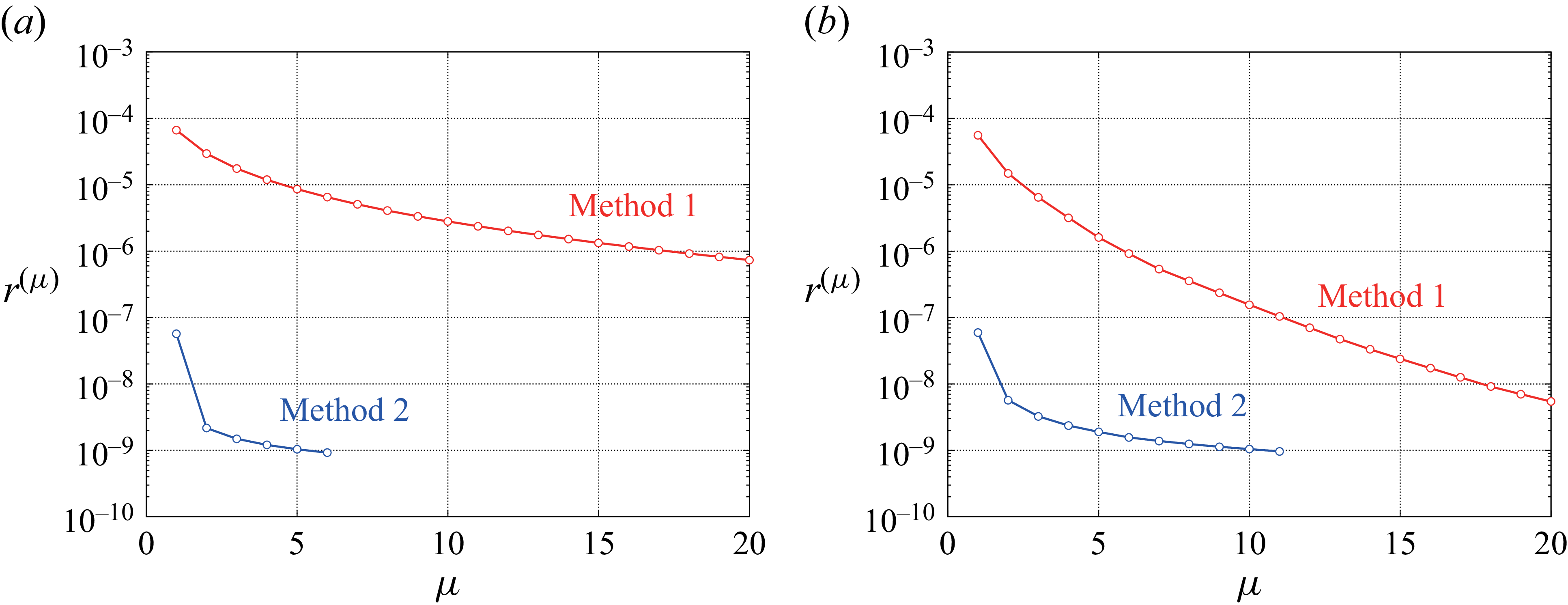
However, the convergence of the iterative scheme (5.10) using the initial guess
 $v^{(0)}$
in (C1) is very slow, as shown in method 1 of figure 8.
Convergence of the iterative scheme (5.10) for two different initial guesses
 $v^{(0)}$
: the residual
 $r^{(\mu )}(t)$
versus the iteration number
 $\mu$
. Method 1 (red line
 ):
 $v^{(0)}$
is given by the linear extrapolation (C1). Method 2 (blue line
 ):
 $v^{(0)}$
is given by the finite difference approximation of (5.9). The residual
 $r^{(\mu )}(t)$
is defined by (5.11). The computed results are obtained using the second-order SNL model for example 1 with
 $\tilde {\alpha }_0 = 0.09$
in § 5.2. See the caption of figure 2 for other parameter values. Results are shown for (
 $a$
)
 $t = 20$
and (
 $b$
)
 $t = 50$
.

On the other hand, we may approximate (5.9) by a system of simultaneous linear equations using the finite difference discretisation of the spatial differentiation of
 $v(x,t)$
with the error of
 $O(\Delta x^4)$
as
 \begin{align} \left . \begin{array}{rcl} v_x(x_j, t) &\!\! \simeq\!\!\! & {\dfrac {v_{\!j-2} - 8 v_{\!j-1} + 8 v_{\!j+1} - v_{\!j+2}}{12 \Delta x}} \\[9pt] v_{\textit{xx}}(x_j, t) &\!\! \simeq\!\!\! & {\dfrac {-v_{\!j-2} + 16 v_{\!j-1} - 30 v_{\!j} + 16 v_{\!j+1} - v_{\!j+2}}{12 \Delta x^2}} \\[9pt] v_{\textit{xxx}}(x_j, t) &\!\! \simeq\!\!\! & {\dfrac {v_{\!j-3} - 8 v_{\!j-2} + 13 v_{\!j-1} - 13 v_{\!j+1} + 8 v_{\!j+2} - v_{\!j+3}}{8 \Delta x^3}} \\[9pt] v_{\textit{xxxx}}(x_j, t) &\!\! \simeq\!\!\! & {\dfrac {-v_{\!j-3} + 12 v_{\!j-2} - 39 v_{\!j-1} + 56 v_j - 39 v_{\!j+1} + 12 v_{\!j+2} - v_{\!j+3}}{6 \Delta x^4}}\end{array} \right \}\!, \end{align}
with
 $v_j = v(x_j, t)$
. Then we adopt a numerical solution of the simultaneous linear equations with the initial guess
 $v^{(0)}$
for the iterative scheme (5.10). Figure 8 shows that method 2 using this initial guess
 $v^{(0)}$
improves convergence of (5.10) considerably.
Appendix D. Fully nonlinear computation using a boundary integral method
This appendix summarises the method of FNL computation for free surface flow over a variable bottom, which is based on a boundary integral method developed by Baker et al. (Reference Baker, Meiron and Orszag1982). Here we assume that the bottom topography is time independent as
 $h = h(x)$
in (5.16) for example 1 and
 $h = h(x,t) = h(X)$
with
 $X = x + F_r t$
in (5.21) for example 2.
First, for the computational domain bounded by
 $-L/2 \lt x \lt L/2$
and
 $-h(x) \lt z \lt \zeta (x,t)$
, we introduce the new complex spatial variables
 $Z = x + \mathrm{i}z$
and
 $\hat {\zeta } = \hat {\xi } + \mathrm{i}\hat {\eta }$
defined by
 \begin{equation} \hat {\zeta } = {\frac {2\pi }{L}} Z \, \, \, \, \, \mbox{with} \, \, \hat {\xi } = {\frac {2\pi }{L}} x , \, \, \hat {\eta } = {\frac {2\pi }{L}} z. \end{equation}
Then the computational domain is given by
 \begin{equation} -\pi \lt \hat {\xi } \lt \pi \, \, \, \, \mbox{and} \, \, \, \, -\check {\eta }(x) \lt \hat {\eta } \lt \tilde {\eta }(x,t) \, , \end{equation}
where
 $\check {\eta }(x) = (2\pi /L) h(x)$
and
 $\tilde {\eta }(x,t) = (2\pi /L) \zeta (x,t)$
. From periodicity, we may parameterise each variable at the free surface
 $z = \zeta (x,t)$
and the bottom
 $z = -h(x)$
and write them, respectively, as
 \begin{align} \hat {\zeta }_{{F}}(p, t) & = \hat {\zeta } \, \, \, \, \mbox{at} \, \, z = \zeta (x,t) \, \, \, \, (-\pi \leqslant p \leqslant \pi ), \end{align}
 \begin{align} \hat {\zeta }_{{B}}(p) & = \hat {\zeta } \, \, \, \, \mbox{at} \, \, z = -h(x) \, \, \, \, (-\pi \leqslant p \leqslant \pi ), \end{align}
where
 $\hat {\zeta }_{{B}}(p) = \hat {\xi }_{{B}}(p) + \mathrm{i} \hat {\eta }_{{B}}(p) = p - \mathrm{i} \check {\eta }_{{B}}(p)$
, namely
 \begin{equation} \hat {\xi }_{{B}}(p) = p, \, \, \hat {\eta }_{{B}}(p) = -\check {\eta }_{{B}}(p) = -\check {\eta }(x = x_{{B}}(p)) \, \, \, \, \mbox{with} \, \, x_{{B}}(p) = {\frac {L}{2\pi }} \hat {\xi }_{{B}}(p) . \end{equation}
Hereafter, the time dependence of each variable is omitted, such as
 $\hat {\zeta }_{{F}}(p)$
instead of
 $\hat {\zeta }_{{F}}(p, t)$
, just for notational brevity if its explicit expression is not necessary. From Cauchy’s integral formula and periodicity, we can write the complex velocity
 $w = w(\hat {\zeta })$
using the vortex-sheet strengths
 $\gamma _{{F}}(p)$
at the free surface and
 $\gamma _{{B}}(p)$
at the bottom, similarly to Baker et al. (Reference Baker, Meiron and Orszag1982, (4.2)), as
 \begin{align} w(\hat {\zeta }) & = {\dfrac {1}{4\pi \mathrm{i}}} {\dfrac {2\pi }{L}} \left \{ {\int _{-\pi }^\pi } \gamma _{{F}}(p^{\prime }) \cot \left [\dfrac {1}{2} \{\hat {\zeta } - \hat {\zeta }_{{F}}(p^{\prime })\}\right ] \mathrm{d}p^{\prime } \right . \nonumber\\ & \quad \left . + \, \mathrm{i} {\int _{-\pi }^\pi } \gamma _{{B}}(p^{\prime }) \cot \left [\dfrac {1}{2} \{\hat {\zeta } - \hat {\zeta }_{{B}}(p^{\prime })\}\right ] \mathrm{d}p^{\prime } \right \}\! . \end{align}
Here note that
 $\gamma _{{F}}(p)$
and
 $\gamma _{{B}}(p)$
are both real and
 \begin{equation} w \, = {\frac {\partial f}{\partial Z}} \, = {\frac {\partial f/\partial p}{\partial Z/\partial p}} \, = {\frac {2\pi }{L}} {\frac {\partial f/\partial p}{\partial \hat {\zeta }/\partial p}} \, , \end{equation}
where
 $f = \phi + \mathrm{i}\psi$
denotes the complex velocity potential. Equation (D5) yields the complex velocities
 $w_{{F}}(p)$
at the free surface and
 $w_{{B}}(p)$
at the bottom, respectively, as
 \begin{align} w_{{F}}(p) = w(\hat {\zeta }_{{F}}(p)) & = {\frac {2\pi }{L}} \left \{ I_{{F}1}(p) + I_{{B}1}(p) + {\frac {1}{2}} {\frac {\gamma _{{F}}(p)}{\partial \hat {\zeta }_{{F}}/\partial p(p)}} \right \}\!, \end{align}
 \begin{align} w_{{B}}(p) = w(\hat {\zeta }_{{B}}(p)) & = {\frac {2\pi }{L}} \left \{ I_{{F}2}(p) + I_{{B}2}(p) - \mathrm{i} {\frac {1}{2}} {\frac {\gamma _{{B}}(p)}{\partial \hat {\zeta }_{{B}}/\partial p(p)}} \right \} , \end{align}
with
 \begin{align} I_{{F}1}(p) & = {\frac {1}{4\pi \mathrm{i}}} \mathrm{P.V.}{\int _{-\pi }^\pi } \gamma _{{F}}(p^{\prime }) \cot \left [\frac {1}{2} \{\hat {\zeta }_{{F}}(p) - \hat {\zeta }_{{F}}(p^{\prime })\}\right ] \mathrm{d}p^{\prime }, \end{align}
 \begin{align} I_{{B}1}(p) & = {\frac {1}{4\pi }} {\int _{-\pi }^\pi } \gamma _{{B}}(p^{\prime }) \cot \left [\frac {1}{2} \{\hat {\zeta }_{{F}}(p) - \hat {\zeta }_{{B}}(p^{\prime })\}\right ] \mathrm{d}p^{\prime }, \end{align}
 \begin{align} I_{{F}2}(p) & = {\frac {1}{4\pi \mathrm{i}}} {\int _{-\pi }^\pi } \gamma _{{F}}(p^{\prime }) \cot \left [\frac {1}{2} \{\hat {\zeta }_{{B}}(p) - \hat {\zeta }_{{F}}(p^{\prime })\}\right ] \mathrm{d}p^{\prime }, \end{align}
 \begin{align} I_{{B}2}(p) & = {\frac {1}{4\pi }} \mathrm{P.V.}{\int _{-\pi }^\pi } \gamma _{{B}}(p^{\prime }) \cot \left [\frac {1}{2} \{\hat {\zeta }_{{B}}(p) - \hat {\zeta }_{{B}}(p^{\prime })\}\right ] \mathrm{d}p^{\prime }, \end{align}
where P.V. denotes Cauchy’s principal value.
The kinematic condition at the free surface is given by
 \begin{equation} {\frac {\partial Z_{{F}}}{\partial t}} = \overline {w}_{{F}} \, \, \, \, \mbox{or} \, \, \, \, {\frac {\partial \hat {\zeta }_{{F}}}{\partial t}} \, = {\frac {2\pi }{L}} \overline {w}_{{F}} \, , \end{equation}
where
 $Z_{{F}} = Z_{{F}}(p,t) = x_{{F}}(p,t) + \mathrm{i} \, z_{{F}}(p,t)$
,
 $\hat {\zeta }_{{F}} = \hat {\zeta }_{{F}}(p,t) = \hat {\xi }_{{F}}(p,t) + \mathrm{i} \, \hat {\eta }_{{F}}(p,t)$
and
 $\overline {w}$
denotes the complex conjugate of
 $w$
. Taking the derivative of the dynamic condition at the free surface given by Bernoulli’s equation with respect to
 $p$
along the free surface, we obtain
 \begin{equation} {\frac {\partial }{\partial t}} \left ( {\frac {\partial \phi _{{F}}}{\partial p}} \right ) - {\frac {1}{2}} {\frac {\partial }{\partial p}}(w_{{F}} \overline {w}_{{F}}) + {\frac {L}{2\pi }} {\frac {\partial \hat {\eta }_{{F}}}{\partial p}} = 0 \, , \end{equation}
where
 $\phi _{{F}}$
denotes the velocity potential at the free surface and
 \begin{equation} {\frac {\partial \phi _{{F}}}{\partial p}} = \mathrm{Re}\left \{ {\frac {\partial f_{{F}}}{\partial p}} \right \} = \mathrm{Re}\left \{ {\frac {\partial Z_{{F}}}{\partial p}} \boldsymbol{\cdot }w_{{F}} \right \} \! . \end{equation}
The bottom condition is given by
 \begin{equation} {\frac {\partial \psi _{{B}}}{\partial p}} = 0, \end{equation}
where
 $\psi _{{B}}$
denotes the streamfunction at the bottom and
 \begin{equation} {\frac {\partial \psi _{{B}}}{\partial p}} = \mathrm{Im}\left \{ {\frac {\partial f_{{B}}}{\partial p}} \right \} = \mathrm{Im}\left \{ {\frac {\partial Z_{{B}}}{\partial p}} \boldsymbol{\cdot }w_{{B}} \right \}. \end{equation}
Note that (D7a ) and (D11) yield
 \begin{equation} \begin{array}{ccl} \gamma _{{F}}(p) & = 2 \left [ {\frac {\partial \phi _{{F}}}{\partial p}} - \mathrm{Re}\left \{ {\frac {\partial \hat {\zeta }_{{F}}}{\partial p}} \boldsymbol{\cdot }\left \{ I_{{F}1}(p) + I_{{B}1}(p) \right \} \right \} \right ] \! . \end{array} \end{equation}
Similarly, (D7b ) and (D13) with (D12) produce
 \begin{equation} \begin{array}{ccl} \gamma _{{B}}(p) & = 2 \boldsymbol{\cdot }\mathrm{Im} \left \{ {\dfrac {\partial \hat {\zeta }_{{B}}}{\partial p}} \boldsymbol{\cdot }\left \{ I_{{F}2}(p) + I_{{B}2}(p) \right \} \right \} \! . \end{array} \end{equation}
In this work, we choose
 $\hat {\zeta }_{{F}}$
and
 $\partial \phi _{{F}}/\partial p$
as the dependent variables, and apply a pseudo-spectral method to the numerical computation of (D9) and (D10), similarly to that for the long wave models in § 5.1. For this, we need to obtain
 $w_{{F}}$
included in (D9) and (D10), which is determined by
 $\gamma _{{F}}$
and
 $\gamma _{{B}}$
, as shown in (D7a
). After solving the evolution equations (D9) for
 $\hat {\zeta }_{{F}}$
and (D10) for
 $\partial \phi _{{F}}/\partial p$
, we can find
 $\gamma _{{F}}$
and
 $\gamma _{{B}}$
at a new time step as follows. The integrals in (D8) can be approximated using the trapezoidal rule and, in particular, Cauchy’s principal value integrals in
 $I_{{F}1}(p)$
and
 $I_{{B}2}(p)$
can be approximated using the alternating trapezoidal rule (Beale, Hou & Lowengrub Reference Beale, Hou and Lowengrub1996, (6)). Then (D14) and (D15) are approximated by a system of simultaneous linear equations for
 $\gamma _{{F}}$
and
 $\gamma _{{B}}$
, which we numerically solve using the successive over-relaxation method.
To estimate the accuracy of this method of FNL computation, we monitor the wave energy
 $E(t)$
, which is the sum of kinetic and potential energies, for the initial cnoidal wave (5.12) with a flat bottom
 $h = h_0$
(
 $L = 60$
,
 $x_0 = -20$
,
 $\Delta t = 0.05$
,
 $N = 2048$
and
 $N_{\textit{filter}} = 400$
). Then it is found that, for the dimensionless wave height
 $\tilde {\alpha }_0 \leqslant 0.18$
, the cnoidal waves propagates in almost permanent form with constant speed
 $\tilde {c}_0$
in (5.15) and the relative error
 $|E(t) - E(0)|/E(0) \lt 0.04\,\%$
.