



1. Introduction
The complex behaviour of fluid–fluid interfaces moving over solid surfaces has captivated the physics community over the past decades (de Gennes Reference de Gennes1985; Bonn et al. Reference Bonn, Eggers, Indekeu, Meunier and Rolley2009; Snoeijer & Andreotti Reference Snoeijer and Andreotti2013), intrigued by the elegant physics of the problem and the multitude of relevant practical applications, such as solid surface coating, CO $_2$ sequestration (MacMinn, Szulczewski & Juanes Reference MacMinn, Szulczewski and Juanes2010, Reference MacMinn, Szulczewski and Juanes2011; Szulczewski et al. Reference Szulczewski, MacMinn, Herzog and Juanes2012), geologic storage of hydrogen (Heinemann et al. Reference Heinemann2021) and design of electrolysers (Lee et al. Reference Lee, Zhao, Abouatallah, Wang and Bazylak2019). One of the important contributions to the problem dates back to 1971 when Huh & Scriven (Reference Huh and Scriven1971) pointed theoretically to a stress-singularity paradox at the intersection of the fluid–fluid interface with the solid (i.e. the contact line). The surge of experimental studies that followed aimed to replicate the physical setting envisioned by Huh and Scriven, where the solid surface was perfectly smooth and homogeneous. Researchers adopted meticulous surface-cleaning protocols intended to minimize chemical and physical defects (de Gennes, Brochard-Wyart & Quéré Reference de Gennes, Brochard-Wyart and Quéré2004), culminating in the experiments of Hoffman (Reference Hoffman1975) that revealed a robust relationship between the shape of the fluid–fluid interface and the displacement rate. This relationship was subsequently rationalized successfully by the hydrodynamic models of Voinov (Reference Voinov1977) and Cox (Reference Cox1986), where a unique interface shape could be inferred from a given displacement rate (a regime henceforth termed steady sliding).
However, most real-world solid surfaces exhibit physical and chemical defects, and fluid–fluid interfaces moving over them can undergo complex intermittent dynamics (Quéré Reference Quéré2008; Zuo et al. Reference Zuo, Zheng, Zhao, Chen, Yan, Ni and Wang2012; Guo et al. Reference Guo, Gao, Xiong, Wang, Wang, Sheng and Tong2013; Varagnolo et al. Reference Varagnolo, Ferraro, Fantinel, Pierno, Mistura, Amati, Biferale and Sbragaglia2013; Perrin et al. Reference Perrin, Lhermerout, Davitt, Rolley and Andreotti2016; Wang et al. Reference Wang, Guo, Chen and Tong2016; Gao et al. Reference Gao, Geyer, Pilat, Wooh, Vollmer, Butt and Berger2018; Hatipogullari et al. Reference Hatipogullari, Wylock, Pradas, Kalliadasis and Colinet2019; Butt et al. Reference Butt2022; Zhang & Xu Reference Zhang and Xu2022; Lindeman & Nagel Reference Lindeman and Nagel2023). The contact line can occasionally pin near strong defects, producing distinct stick–slip motion of the interface, where one-to-one mapping between the interface shape and the displacement rate is no longer possible. The force–velocity scaling of such motion is also distinct from one on smooth substrates; it depends on whether the displacement is driven at a constant rate or with a constant force (Raphaël & De Gennes Reference Raphaël and De Gennes1989; Joanny & Robbins Reference Joanny and Robbins1990).
A viscous slug moving inside a capillary tube can exhibit both stick–slip and steady sliding motion, depending on the displacement rate (figure 1). The slug dynamics resemble the frictional sliding of a solid block, where the transition from stick–slip to steady sliding has been researched thoroughly (Brace & Byerlee Reference Brace and Byerlee1966; Rice & Tse Reference Rice and Tse1986; Alghannam & Juanes Reference Alghannam and Juanes2020), and the results have been used to inform our understanding of earthquakes. The rate effects on stick–slip motion have also been examined in adhesive tapes (Maugis & Barquins Reference Maugis and Barquins1988) and granular materials (Nasuno et al. Reference Nasuno, Kudrolli, Bak and Gollub1998). In contrast, no simple relation is known that marks the transition from stick–slip to steady sliding in a viscous slug – a physical situation abundant in multiphase flow in porous media and microfluidics applications. Filling this gap is the primary objective of our theoretical study.
(a) Schematic of a viscous slug, where only the water–oil meniscus is partially wetting and therefore interacts with surface defects. (b) The constant-force experiment can be realized by imposing a fixed pressure difference across the viscous slug (neglecting the pressure gradient in water) by controlling the reservoir height  $\Delta {h}$. (c) The constant-rate experiment can be realized by supplying water through a syringe at a prescribed flow rate. (d) A slug of viscous oil displaced by water inside an NOA81-coated capillary tube crosses over from stick–slip motion (left) to steady sliding (right) as the displacement rate increases. Both experiments were driven at a constant rate. The low-velocity experiment was at
 ${Ca}=2.35\times 10^{-3}$, while the high-velocity experiment was at
 ${Ca}=2.31\times 10^{-2}$. Here, we define a capillary number as
 ${Ca}={\mu \dot {z}_c}/{\gamma _{ow}}$. See the Appendix for experimental details.

Here, we reduce the dynamics of a viscous slug motion to a system of coupled ordinary differential equations, whose form is equivalent to equations of motion by Raphaël & De Gennes (Reference Raphaël and De Gennes1989) and Joanny & Robbins (Reference Joanny and Robbins1990). We recast these equations in a periodic domain, connecting them to a fluid-filled drum analogue of Adler (Reference Adler1946). While the link between constant-force displacement and Adler's analogue has been recognized by Thiele & Knobloch (Reference Thiele and Knobloch2006a,Reference Thiele and Knoblochb), we extend Adler's analogue to the constant-rate displacement setting. Doing so allows the reduction of the complexity of stick–slip dynamics to a few key parameters, elucidating both constant-force and constant-rate displacement regimes. While the work of Raphaël & De Gennes (Reference Raphaël and De Gennes1989) and Joanny & Robbins (Reference Joanny and Robbins1990) focused on the force–velocity scaling at diminishing displacement rates, ours provides a rationale for the crossover between stick–slip and steady sliding motion at high displacement rates. This transition is characterized by a simple scaling relation between the spacing of the defects, the characteristic size of the fluid–fluid interface, and the capillary number – a scaling relation that can help to explain disparate stick–slip phenomenology from recent experimental studies.
We develop the equations of motion for the viscous slug in § 2. We examine the transition from stick–slip to steady sliding in constant-force (§ 3) and constant-rate (§ 4) settings, presenting the scaling relation for the crossover, and discussing implications for total force (§ 5), energy dissipation (§ 6) and motion over disordered pinning landscapes (§ 7). We compare our results to a phase-field simulation in § 8 and conclude in § 9 by discussing the connection of our theoretical results to recent experimental studies.
2. Physical set-up and governing equations
Consider a viscous silicone oil slug of length  $l$ being displaced by water inside a capillary tube with inner radius
 $R$, whose surface is not perfectly smooth or homogeneous (figure 1a). Here,
 $\theta _b$ and
 $\theta _f$ are water–oil and oil–air contact angles, and
 $z_b$ and
 $z_c$ are the positions of the water–oil meniscus centre and the contact line along the tube. We chose a silicone oil with viscosity much greater than the viscosity of water (
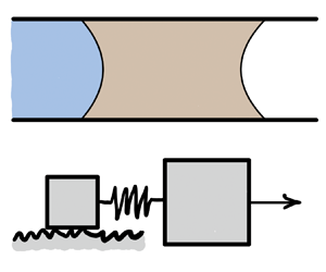
 $\mu _o \gg \mu _w$), which allows neglecting pressure gradients outside the slug. Furthermore, only the partially wetting water–oil interface interacts with the surface imperfections; the oil–air interface is in complete wetting, where a precursor film (or hemi-wicking front) masks surface defects (Joanny & Robbins Reference Joanny and Robbins1990). One can drive the viscous slug at either constant force (figure 1b) or constant rate (figure 1c). At low velocity, the slug moves through stick–slip motion, while at high velocity, it experiences steady sliding (figure 1d). This is reminiscent of a solid block being pulled through a spring (a spring–slider model, figure 1a). However, while the transition from stick–slip to steady sliding is controlled by the stiffness of the spring in the spring–slider, the analogous transition in viscous slugs seems to be controlled by the displacement rate.
To rationalize the transition from stick–slip to steady sliding, we simplify the system in figure 1(a), producing governing equations identical to the ones in the depinning dynamics framework by Raphaël & De Gennes (Reference Raphaël and De Gennes1989) and Joanny & Robbins (Reference Joanny and Robbins1990). In fact, by forcing the viscous slug at either constant force (figure 1b) or constant rate (figure 1c), one can probe experimentally the seminal force–velocity scaling relations proposed by Raphaël & De Gennes (Reference Raphaël and De Gennes1989) and Joanny & Robbins (Reference Joanny and Robbins1990). Here, we examine how the governing equations behave away from the depinning limit, and rationalize the transition from stick–slip to steady motion for both constant-rate and constant-force settings.
The overall motion results from a balance of several forces. We express the externally applied force through the pressure difference  $\Delta {p}$ at the two ends of the slug as
 \begin{equation} F_{ext}=\Delta{p}\,{\rm \pi} R^2. \end{equation}
The bulk viscous force exerted on the slug due to Poiseuille flow is
 \begin{equation} F_{v.bulk}=8{\rm \pi}\mu_o l \dot{z}_b. \end{equation}
Here, we assume that the length of the slug  $l$ is independent of time, as was the case in Primkulov et al. (Reference Primkulov, Chui, Pahlavan, MacMinn and Juanes2020a). This implies that the oil slug does not leave behind a film of oil on the tube walls (see the Appendix). Since the front meniscus is completely wetting, its capillary force can be approximated with
 \begin{equation} F_f \approx 2{\rm \pi} R \gamma_o, \end{equation}
where we neglected the dynamic contribution of  $F_f$, assuming a sufficiently long slug (Primkulov et al. Reference Primkulov, Chui, Pahlavan, MacMinn and Juanes2020a). We model the chemical heterogeneity of the solid surface by a spatially periodic perturbation
 $h(z_c)$ to a spreading coefficient (Raphaël & De Gennes Reference Raphaël and De Gennes1989; Joanny & Robbins Reference Joanny and Robbins1990), which is equivalent to
 \begin{equation} \cos\theta_b=\cos\theta_{b0}+h(z_c)/\gamma_{ow}, \end{equation}
where  $\theta _{b0}$ is the contact angle on an ideally smooth and homogeneous surface. For simplicity, we assume
 $\theta _{b0}={\rm \pi} /2$ and neglect the viscous bending of the interface in both the front and back menisci. We can then treat the water–oil interface as a linear spring, with
 \begin{equation} F_{sp} = 2{\rm \pi} R k(z_b-z_c), \end{equation}
and the spring constant can be approximated as  $k=\gamma _{ow}/R$. Finally, we approximate the local viscous force of the back meniscus as a cumulative force of moving wedge-shaped fluid slices with contact angle
 $\theta _{b0}$ (de Gennes Reference de Gennes1985; Joanny & Robbins Reference Joanny and Robbins1990; Golestanian Reference Golestanian2004):
 \begin{equation} F_{v.b} \approx 2{\rm \pi} R\,\frac{3\varGamma\mu_o}{{\rm \pi}-\theta_{b0}}\,\dot{z_c} \approx 2{\rm \pi} R\, \frac{6\varGamma\mu_o}{\rm \pi}\,\dot{z_c}, \end{equation}
where  $\varGamma$ is the logarithmic factor of order one (de Gennes Reference de Gennes1985). In (2.6),
 $F_{v.b} \sim \dot {z_c}$ means that the water–oil contact line acts similarly to a viscous dashpot in the classic spring–slider model. We can then write down the coupled dynamics of the slug and the back contact line as
 $$\begin{gather} F_{v.bulk} = F_f + F_{ext} - F_{sp}, \end{gather}$$
 $$\begin{gather}F_{v.b} = F_{sp} + 2{\rm \pi} R\,h(z_c). \end{gather}$$
Equations (2.7)–(2.8) reduce to
 $$\begin{align} \overbrace{b_b \dot{z_b}}^{\textit{slug dashpot}} &=\overbrace{f}^{\textit{applied force}}-\overbrace{k(z_b-z_c)}^{\textit{coupling spring}}, \end{align}$$
 $$\begin{align}\underbrace{b_c \dot{z_c}}_{\textit{contact-line dashpot}} &=k(z_b-z_c)+\underbrace{h(z_c)}_{\textit{pinning force}}, \end{align}$$
where  $b_b=4\mu _o l/R$,
 $b_c=6\varGamma \mu _o/{\rm \pi}$ and
 $f=\gamma _o +\Delta {p}\,R/2$.
Following Joanny & Robbins (Reference Joanny and Robbins1990), we model heterogeneity in the spreading coefficient with a sine function as this minimal model still allows us to capture the essential physics of interest here. Therefore,
 \begin{equation} h(z_c) ={-}\epsilon\gamma_{ow}\sin(2{\rm \pi} z_c/q), \end{equation}
where  $\epsilon <1$, and
 $q$ is the distance between consecutive peaks of the sine function. We write down the system (2.9)–(2.10) in a reduced form by defining
 $\alpha =2{\rm \pi} z/q$ as
 $$\begin{gather} \dot{\alpha_b} = \overbrace{\omega_0}^{\textit{force term}} - \overbrace{K(\alpha_b-\alpha_c)}^{\textit{spring term}}, \end{gather}$$
 $$\begin{gather}\lambda\dot{\alpha}_c = K(\alpha_b-\alpha_c) - \underbrace{B\sin\alpha_c}_{\textit{pinning term}}, \end{gather}$$
where  $\lambda =b_c/b_b$,
 $\omega _0=2{\rm \pi} f/b_b q$,
 $K=k/b_b$ and
 $B=2{\rm \pi} \gamma _{ow}\epsilon /b_b q$. This dynamical system has two interacting parts: bulk motion of the slug and the local motion of the water–oil contact line. These two parts interact through a spring (water–oil interface). One can drive this system either at a constant force (by fixing
 $\omega _0$) or at a constant rate (by imposing
 $\dot {\alpha }_b=\omega _u$). It is important to note that
 $\lambda \sim R/l$ (see table 1) is a small parameter since we assumed that our viscous slug is slender.
Conversions between key parameters of the drum analogue and physical parameters in a capillary tube, where coefficients have been dropped for clarity.

The connection of our model to the models of Raphaël & De Gennes (Reference Raphaël and De Gennes1989) and Joanny & Robbins (Reference Joanny and Robbins1990) deserves a note. Our (2.9)–(2.10) are identical to the governing equations in Raphaël & De Gennes (Reference Raphaël and De Gennes1989) (Eqs 2.4 and 2.7, respectively, in their paper). Therefore, it is not surprising that our model is able to reproduce key results from Raphaël & De Gennes (Reference Raphaël and De Gennes1989) and Joanny & Robbins (Reference Joanny and Robbins1990); we do so for completeness in our work. However, we take one step further – recasting the governing equations in the form (2.12)–(2.13) allows us to connect our system to mechanical analogues in figure 2, and express the dynamics in only three dimensionless groups in §§ 3 and 4. In § 3, we first reproduce the force–velocity scaling results from the adiabatic approximation of Raphaël & De Gennes (Reference Raphaël and De Gennes1989) and Joanny & Robbins (Reference Joanny and Robbins1990). We then relax the adiabatic approximation and explore how the system behaves in this yet unexplored parameter regime. Similarly, we begin § 4 by reproducing the force–velocity scaling results of Raphaël & De Gennes (Reference Raphaël and De Gennes1989) and Joanny & Robbins (Reference Joanny and Robbins1990) for the constant-rate setting in the presence of disanchoring events. We extend this analysis by including the force–velocity relations in the absence of disanchoring events. However, this work's central contribution is exploring the transition from stick–slip to steady sliding motion in both constant-force (§ 3) and constant-rate (§ 4) settings, where the analogues depicted in figure 2 provide a natural framework.
Mechanical analogue of the spring oscillator model in a constant-force regime (a) moves through either stick–slip (b) or steady motion (c). This analogue can be extended to a constant displacement regime by introducing a spring that is pulled at constant angular velocity  $\omega _u$ (d). Here, the pendulum also moves through either stick–slip (e) or steady motion ( f). The shading of the pendulum represents a time sequence, where lighter colours refer to past pendulum positions.

3. Constant-force analogue
When the system is driven at a constant force,  $\omega _0$ is fixed in (2.12). We can then rescale the time as
 $\tau =\omega _0 t$ to obtain a dimensionless form of the governing equations,
 $$\begin{gather} \dot{\alpha_b} = 1 - \frac{K}{\omega_0}\,(\alpha_b-\alpha_c), \end{gather}$$
 $$\begin{gather}\lambda\dot{\alpha}_c = \frac{K}{\omega_0}\,(\alpha_b-\alpha_c) - \frac{B}{\omega_0}\sin\alpha_c, \end{gather}$$
where three dimensionless groups ( $\lambda$,
 $K/\omega _0$ and
 $B/\omega _0$) emerge. Here,
 $\lambda$ is the ratio of contact-line to slug damping coefficients, while
 $K/\omega _0$ and
 $B/\omega _0$ represent the importance of spring and pinning forces relative to the driving force.
3.1. Special case ( $\lambda \ll 1$ and $B/K \ll 1$)


We first consider a special case that offers valuable physical insights into the problem. When  $\lambda \ll 1$ (contact-line damping
 $\ll$ slug damping), we can neglect the
 $\lambda \dot {\alpha }_c$ term, so (3.1)–(3.2) reduce to
 $\dot {\alpha }_b = 1 - ({B}/{\omega _0})\sin \alpha _c$ and
 $\dot {\alpha }_b = (1+({B}/{K})\cos \alpha _c)\dot {\alpha }_c$. By eliminating
 $\dot {\alpha }_b$, one can obtain
 \begin{equation} \dot{\alpha}_c = \frac{1 - \dfrac{B}{\omega_0}\sin\alpha_c}{1+\dfrac{B}{K}\cos\alpha_c}, \end{equation}
which simplifies to
 \begin{equation} \dot{\alpha}_c = 1 - \frac{B}{\omega_0}\sin\alpha_c \end{equation}
when  $B/K \ll 1$ (pinning
 $\ll$ spring term). This corresponds to the adiabatic approximation of Raphaël & De Gennes (Reference Raphaël and De Gennes1989) and Joanny & Robbins (Reference Joanny and Robbins1990). In fact, (3.4) emerges in many dynamical systems; Strogatz (Reference Strogatz2018) discusses this equation in relation to firefly synchronization and Josephson junction problems, while Adler (Reference Adler1946) examined it in the context of locking phenomena in electric oscillators. Adler (Reference Adler1946) proposed an overdamped pendulum analogue that we will use to understand our system.
Consider a pendulum inside a drum filled with viscous fluid, where the drum is rotated at a fixed angular velocity  $\omega _0$, and
 $-B\sin \alpha _c$ is the gravity term acting on the pendulum (figure 2a). As one increases
 $\omega _0$ gradually, the system undergoes several distinct regimes.
3.1.1. Static limit ($B/\omega _0 \geq 1$)

The pendulum acquires a static angle  $\alpha _c$ when the applied force is insufficient to overcome gravity (
 $B/\omega _0>1$). Here, (3.4) has one stable and one unstable fixed point:
 \begin{equation} \alpha_c^* = \arcsin(B/\omega_0) \quad \text{and} \quad \alpha_c^* = {\rm \pi}-\arcsin(B/\omega_0). \end{equation}
The stable fixed point represents a pinned state of the viscous slug, where local imperfections match the driving force. These two fixed points coalesce to  $\alpha _c={\rm \pi} /2$ at
 $B/\omega _0 = 1$, and disappear as
 $B/\omega _0$ decreases below
 $1$.
3.1.2. Dynamic limit ($B/\omega _0 \rightarrow 1^-$)

When  $\omega _0$ is infinitesimally greater than
 $B$, the pendulum goes through distinct stick–slip motion; it is slower when moving against gravity, and faster when moving in the direction of gravity (figure 2b). We can rearrange and integrate (3.4) to calculate the period of the pendulum (Strogatz Reference Strogatz2018):
 \begin{equation} T=\int_0^{2{\rm \pi}}\frac{{\rm d}\alpha_c}{1-\dfrac{B}{\omega_0}\sin{\alpha_c}} = \frac{2{\rm \pi}}{\sqrt{1-B^2/\omega_0^2}}, \end{equation}
which blows up as  $B/\omega _0$ approaches 1. The pendulum spends most of its period near
 $\alpha _c = {\rm \pi}/2$, corresponding to the maximum of the gravity term. This regime corresponds to the stick–slip motion of the viscous slug near the depinning limit.
The average frequency of the pendulum is (Adler Reference Adler1946)
 \begin{equation} \frac{\bar{\omega}}{\omega_0}=\sqrt{1-B^2/\omega_0^2}. \end{equation}
When  $B/\omega _0 \rightarrow 1^-$,
 \begin{align}
\frac{\bar{\omega}}{\omega_0}&=\sqrt{\bigg[\bigg(1-\frac{B}{\omega_0}\bigg)+\frac{B}{\omega_0}\bigg]^2
-\frac{B^2}{\omega_0^2}} =
\sqrt{\frac{2B}{\omega_0}\bigg(1-\frac{B}{\omega_0}\bigg)+\bigg(1-\frac{B}{\omega_0}\bigg)^2}\nonumber\\
&\approx \sqrt{\frac{2B}{\omega_0}\bigg(1-\frac{B}{\omega_0}\bigg)}.
\end{align}
We can therefore write the force–velocity relation near the depinning limit as
 \begin{equation} \frac{\omega_0-B}{B} = \frac{1}{2}\left(\frac{\bar{\omega}}{B}\right)^2, \end{equation}
which is equivalent to the expressions obtained by Raphaël & De Gennes (Reference Raphaël and De Gennes1989) and Joanny & Robbins (Reference Joanny and Robbins1990). In fact, (3.9) can be obtained from (3.6) after realizing that when  $B/\omega _0 \rightarrow 1^-$, the dominant contribution to the integral in (3.6) comes from the neighbourhood of the strongest pinning site.
3.1.3. Transition to steady sliding ($B/\omega _0 \ll 1$)

When  $\omega _0 \gg B$, (3.7) simply reduces to
 $\bar {\omega } = \omega _0$, which we can rewrite in a form analogous to (3.9):
 \begin{equation} \frac{\omega_0-B}{B} \sim \frac{\bar{\omega}}{B}. \end{equation}
Away from the depinning limit, force scales linearly with speed. The numerical results of the force–velocity scaling for the constant-force analogue are shown in figure 4(a).
When  $\omega _0 \gg B$, the viscous fluid within the drum sweeps up the pendulum (figure 2c), and its mean angular velocity
 $\bar {\omega }$ approaches
 $\omega _0$. Figures 3(a,b) show that as one moves away from the depinning limit, the amplitude of oscillations diminishes in a frame moving at
 $\bar {\omega }/\omega _0$. In fact, if we take
 $\tilde {\alpha }_c = \alpha _c - ({\bar {\omega }}/{\omega _0})\tau$, then we can rewrite (3.4) in this moving frame as
 \begin{equation} \frac{{\rm d}\tilde{\alpha}_c}{{\rm d}\tau} = 1 - \frac{\bar{\omega}}{\omega_0} - \frac{B}{\omega_0}\sin\left(\widetilde{\alpha_c}+\frac{\bar{\omega}}{\omega_0}\,\tau\right) \approx{-}\frac{B}{\omega_0}\sin(\tau), \end{equation}
where we took the limit  ${\bar {\omega }}/{\omega _0} \rightarrow 1$ and assumed
 $\tilde {\alpha }_c \ll \tau$. This allows approximating the oscillations about the moving frame as
 \begin{equation} \tilde{\alpha}_c(\tau) \approx \overbrace{\frac{B}{\omega_0}}^{{amplitude}}\cos(\tau) + C. \end{equation}
In other words, we expect the amplitude of oscillations to decay with increasing  $\omega _0$, following
 $B/\omega _0$ scaling, which is indeed what we observe in the numerical solution to (3.4) (figure 5).
Evolution of (a)  $\alpha _c$ and (b)
 $\dot {\alpha }_c$ for the special case (§ 3.1) of the constant-force analogue. Here,
 $\omega _0/B \in (1,2]$,
 $B/K \ll 1$, and the motion is governed by (3.4). Evolution of (c)
 $\alpha _c$ and (d)
 $\dot {\alpha }_c$ for the general case (§ 3.2) of the constant-force analogue. Here,
 $\omega _0/B \in (1,2]$,
 $B/K = 0.9$, and the motion is governed by (3.1)–(3.2).

3.2. General case
If we relax the condition that  $B/K \ll 1$, then we see that the pendulum speed
 $\dot {\alpha }_c$ can blow up as
 $B/K \rightarrow 1$ in (3.3). Hence neglecting the
 $\lambda \dot {\alpha }_c$ term is no longer justified, and one has to consider (3.1)–(3.2) to resolve the dynamics.
Fixed points ( $\alpha _b^*,\alpha _c^*$) of the general case are identical to those in § 3.1 and correspond to
 $$\begin{gather} 0= 1 - \frac{K}{\omega_0}\,(\alpha_b^*-\alpha_c^*), \end{gather}$$
 $$\begin{gather}0= \frac{K}{\omega_0}\,(\alpha_b^*-\alpha_c^*) - \frac{B}{\omega_0}\sin\alpha_c^*, \end{gather}$$
or simply  $({B}/{\omega _0})\sin \alpha _c^* = 1$. Therefore, as in § 3.1, the system is static whenever
 $B/\omega _0 \geq 1$, and undergoes a depinning transition when
 $B/\omega _0 \rightarrow 1^-$, which produces distinct stick–slip events of the contact line (figures 3c,d). Increasing
 $\omega _0$ away from the depinning limit reduces the amplitude of contact-line oscillations in the frame moving at the mean displacement rate
 $\bar {\omega }/\omega _0$ (see figure 3c). Here,
 $\bar {\omega }$ no longer follows (3.7), and is instead evaluated numerically from the period of
 $\alpha _c(\tau )$. Interestingly, the force–velocity scaling relations from § 3.1 hold up for arbitrary
 $B/K$ (figure 4b). Figure 4 demonstrates that both simplified and general cases of the constant-force analogue cross over to a linear force–velocity regime when
 \begin{equation} \frac{\omega_0-B}{B} \sim 1. \end{equation}
This, however, does not correspond to the transition from stick–slip to steady sliding, as the relation between the amplitude of oscillations depends non-trivially on the parameter  $B/K$ (see figure 5b). In figure 5(b), the amplitude of oscillations for fixed
 $B/K$ initially decays rapidly, then undergoes a plateau region starting at
 $\omega _0/B \sim {1}/{(B/K)}$, and ultimately decays again after
 $\omega _0/B \sim {1}/{(\lambda B/K)}$. This trend can be rationalized readily by considering two limits of the governing equations (3.1)–(3.2).


Diminishing amplitude of oscillations with  $\omega _0/B$ in (a) the special case (§ 3.1) and (b) the general case (§ 3.2) of the constant-force setting. (c) The amplitude data from part (b) are replotted as a function of
 $\lambda \omega _0/K$, where the dashed line corresponds to the crossover from stick–slip to steady sliding. Data correspond to numerical solutions of (a) (3.4) and (b) (3.1)–(3.2) at varying
 $\omega _0/B$.

When the term  $\lambda \dot {\alpha }_c$ is negligible in (3.1)–(3.2), one can approximate the dynamics with (3.3). In this case, an argument analogous to one in § 3.1.3 leads to
 \begin{equation} \tilde{\alpha}_c(\tau) = \frac{B}{K}\sqrt{1+\frac{K^2}{\omega_0^2}}\sin(\tau+\arctan(\omega_0/K)). \end{equation}
This equation shows that the amplitude of oscillations would first decay following  $B/\omega _0$ scaling and then settle into a
 $B/K$ plateau as
 $\omega _0/B$ increases in figure 5(b). The onset of this plateau coincides with
 ${K}/{\omega _0} \sim 1$, which is equivalent to
 $\omega _0/B \sim {1}/{(B/K)}$.
The extent of the plateau region in figure 5(b) can be estimated by considering a limit where  $({B}/{\omega _0})\sin \alpha _c$ becomes negligible compared to all other terms in (3.1)–(3.2). In this limit, the governing equations can be reduced to
 \begin{equation} \frac{{\rm d}}{{\rm d}\tau}(\alpha_b-\alpha_c) + \frac{K}{\lambda\omega_0}\,(\alpha_b-\alpha_c) = 1, \end{equation}
whose solution is
 \begin{equation} \alpha_b-\alpha_c = \frac{\lambda \omega_0}{K} + C \,{\rm e}^{-({K}/{\lambda\omega_0})\tau}. \end{equation}
In other words, the distance between  $\alpha _b$ and
 $\alpha _c$ starts increasing with
 $\omega _0$. This effect becomes significant when
 $\lambda \omega _0/K \sim 1$ or, equivalently,
 $\omega _0/B \sim {1}/{(\lambda B/K)}$. In this limit, (3.2) can be approximated as
 \begin{equation} \lambda\dot{\alpha}_c = \lambda - \frac{B}{\omega_0}\sin\alpha_c, \end{equation}
whose solution decays with  $\omega _0/B$. This corresponds to the post-plateau decay of amplitude in figure 5(b).
A non-trivial dependence of the amplitude of oscillations on  $B/K$ in figure 5(b) makes it challenging to pinpoint a single condition for the transition from stick–slip to steady sliding motion for the general case of the constant-force analogue. If, however, the parameter
 $B/K \sim O(1)$, then one can take
 \begin{equation} \frac{\lambda\omega_0}{K} \sim 1 \end{equation}
as a condition for the crossover from stick–slip to steady sliding (i.e. the end of the plateau region). In fact, replotting the data in figure 5(b) with  ${\lambda \omega _0}/{K}$ on a horizontal axis confirms that the amplitude of oscillations decays for all
 $B/K$ when
 ${\lambda \omega _0}/{K} > 1$ (figure 5c). On the other hand, if
 $B/K \ll O(1)$, then the amplitude of oscillations becomes negligible before even reaching the plateau in figure 5(b). Hence condition (3.20) is too conservative for this case.
4. Constant-rate analogue
When the viscous slug is driven at a constant rate  $\dot {\alpha }_b=\omega _u$, a modified version of the drum analogue still holds. In the constant-rate analogue, the drum is free, while the pendulum is pulled at a fixed angular velocity
 $\omega _u$ through a spring (figures 2d–f). It is useful to switch to a frame moving with the viscous slug. In this coordinate system,
 ${{\rm d}\tilde {\alpha }_b}/{{\rm d}t}=0$ and we can choose the frame in a way such that
 $\tilde {\alpha }_b=0$, so (2.12)–(2.13) transform to
 $$\begin{gather} \omega_0-\omega_u ={-}K\tilde{\alpha}_c, \end{gather}$$
 $$\begin{gather}\underbrace{\lambda\,\frac{{\rm d}\tilde{\alpha}_c}{{\rm d}t}}_{\textit{dynamic term}} + \underbrace{K\tilde{\alpha}_c}_{\textit{spring}} ={-}\underbrace{B\sin(\tilde{\alpha}_c+\omega_u t)}_{\textit{pinning}}, \end{gather}$$
where  $\omega _0-\omega _u$ is the force term due to loading of the spring, and the pendulum motion is governed by (4.2). The dimensionless form of the above equations is obtained by scaling the time as
 $\tau =\omega _u t$:
 $$\begin{gather} \frac{\omega_0}{\omega_u}-1 ={-}\frac{K}{\omega_u}\,\tilde{\alpha}_c, \end{gather}$$
 $$\begin{gather}\lambda\,\frac{{\rm d}\tilde{\alpha}_c}{{\rm d}\tau} + \frac{K}{\omega_u}\,\tilde{\alpha}_c ={-}\frac{B}{\omega_u}\sin(\tilde{\alpha}_c+\tau), \end{gather}$$
where three dimensionless groups ( $\lambda$,
 $K/\omega _u$,
 $B/\omega _u$) set the dynamics (see table 1). Unlike the constant-force displacement, as long as the prescribed rate is not zero, the pendulum does not have a static state.
4.1. Quasi-static limit
In the quasi-static limit, we can neglect  $\lambda ({{\rm d}\tilde {\alpha }_c}/{{\rm d}\tau })$, and (4.4) reduces to
 \begin{equation} \frac{K}{\omega_u}\,\tilde{\alpha}_{c.qs} ={-}\frac{B}{\omega_u}\sin(\tilde{\alpha}_{c.qs}+\tau). \end{equation}
Therefore, the position of the pendulum is determined by the balance of a linear spring and a sinusoidal gravity term, where the graphical solution for  $\tilde {\alpha }_c$ is the intersection of the respective functions (Raphaël & De Gennes Reference Raphaël and De Gennes1989) (see figures 6a,d). Here, two distinct modes of motion emerge. If the slope of
 $K\tilde {\alpha }_c$ is greater than the maximal slope of
 $-B\sin (\tilde {\alpha }_c+\tau )$ (or
 $K>B$), then the red line (which shifts to the left with time) and the blue line in figure 6(d) intersect only once at any given time. This results in a relatively smooth motion of the pendulum. On the other hand, when
 $K< B$, the two functions intersect more than once. An abrupt change in
 $\tilde {\alpha }_c$ takes place whenever the system moves past the point where spring and pinning functions are tangent to each other (i.e. the disanchoring configuration depicted in figure 6a).
(a) Quasi-static motion of the pendulum in the constant-rate displacement is governed by the balance between spring and gravity terms, where the latter shifts left with time. When  $B>K$, two lines occasionally intersect more than once, which results in disanchoring events depicted here. (b) Evolution of
 $\tilde {\alpha }_c$ from the numerical solution of (4.4) for
 $\omega _u/B \in [10^{-1},10^{2}]$ and
 $B/K=2.3$ shows that the amplitude of
 $\tilde {\alpha }_c$ vanishes as the rate
 $\omega _u$ increases. (c) The speed of the pendulum
 $\dot {\tilde {\alpha }}_c$ can significantly exceed
 $O(1)$ near the quasi-static limit. (d) When
 $B< K$ (
 $B/K = 0.57$), spring and pinning functions can intersect only once. (e) This produces smooth motion of the pendulum (
 $\omega _u/B \in [10^{-1},10^{2}]$ and
 $B/K=0.6$), where ( f)
 $\dot {\tilde {\alpha }}_c \sim O(1)$.

We can calculate the average force term of the quasi-static displacement as
 \begin{equation} \frac{\bar{\omega}_{0.qs}}{\omega_u} = 1 - \frac{1}{T} \int_0^{T} \frac{K}{\omega_u}\, \tilde{\alpha}_{c.qs}(\tau) \,{\rm d}\tau, \end{equation}
where  $T=2{\rm \pi}$ is the period of motion and
 $\tilde {\alpha }_{c.qs}(\tau )$ is calculated from (4.5).
4.2. Dynamic limit for moderate/strong pinning ($K< B$)

We now examine how the average force term evolves as we increase  $\omega _u$ and therefore moves away from the quasi-static approximation when
 $K< B$. Figure 7(a) shows the typical
 $\tilde {\alpha }_c(\tau )$ profile obtained by solving (4.4). We are particularly interested in the dynamics near the disanchoring event highlighted in green. Here, in the quasi-static limit,
 $\tilde {\alpha }_{c.qs}(\tau )$ experiences a jump discontinuity. In the dynamic model, this discontinuity is regularized by the viscous term in (4.4). In fact, the solution of (4.4) deviates from the quasi-static solution only immediately after these disanchoring events (see figure 7b). This deviation is responsible for the force–velocity scaling near the depinning limit of Raphaël & De Gennes (Reference Raphaël and De Gennes1989) and Joanny & Robbins (Reference Joanny and Robbins1990).
(a) Typical motion near the depinning limit, where the quasi-static solution experiences a jump discontinuity in  $\tilde {\alpha }_c$. (b) Expanded view of the region highlighted in green in (a). Solution of (4.4) (blue curve,
 ${\omega _u/B=10^{-2}}$,
 $B/K=2.3$) deviates from the quasi-static profile
 $\tilde {\alpha }_{c.qs}$ (red curve) only near the disanchoring event; area between the curves (grey) corresponds to the integral in (4.8). (c) Solution to (4.14) (blue) as well as the quasi-static solution
 $\hat {\alpha }_{q.s}(\hat {t}) = -\sqrt {-\hat {t}}$ (red). Here,
 $\hat {t}_1$ is the first root of (4.17), and
 $\hat {t}_2$ is its first singularity.

We can write the average force term from (4.3) as
 \begin{equation} \frac{\bar{\omega}_{0}}{\omega_u} = 1 - \frac{1}{T} \int_0^T \frac{K}{\omega_u}\, \tilde{\alpha}_{c}(\tau) \,{\rm d}\tau, \end{equation}
or alternatively we can use (4.6) to rewrite the above equation as
 \begin{equation} \frac{\bar{\omega}_{0} - \bar{\omega}_{0.qs}}{\omega_u} ={-} \frac{1}{T} \int_0^T \frac{K}{\omega_u}\, [\tilde{\alpha}_{c}(\tau)-\tilde{\alpha}_{c.qs}(\tau)] \,{\rm d}\tau. \end{equation}
The value of this integral is equal to the area between the two curves in figure 7(b), and can be approximated as an area of a rectangle if one finds its characteristic width in  $\tau$. This is what we do next.
To understand how  $\tilde {\alpha }_c$ evolves near the disanchoring point
 $(\tau _d,\alpha _d)$, we substitute
 $\tau =\tau _d+\tau _\epsilon$ and
 $\tilde {\alpha }_c = \alpha _d + \alpha _\epsilon$ into (4.4) and obtain
 \begin{equation} \lambda\,\frac{{\rm d}\alpha_\epsilon}{{\rm d}\tau_\epsilon} + \frac{K}{\omega_u}\,(\alpha_d+\alpha_\epsilon) ={-}\frac{B}{\omega_u}\sin(\alpha_d+\tau_d + \alpha_\epsilon+ \tau_\epsilon). \end{equation}
We then note that  $\sin (\alpha _d+\tau _d + \alpha _\epsilon +\tau _\epsilon )=\sin (\alpha _d+\tau _d)\cos (\alpha _\epsilon +\tau _\epsilon )+\cos (\alpha _d+\tau _d)$
 $\sin (\alpha _\epsilon +\tau _\epsilon ) \approx \sin (\alpha _d+\tau _d)\,(1-(\alpha _\epsilon +\tau _\epsilon )^2/2) + \cos (\alpha _d+\tau _d)\,(\alpha _\epsilon +\tau _\epsilon )$. We also note that at the disanchoring point,
 $-B\sin (\alpha _d+\tau _d)=K\alpha _d$ and
 $-B\cos (\alpha _d+\tau _d)=K$. Therefore, (4.9) simplifies to
 \begin{equation} \lambda\,\frac{{\rm d}\alpha_\epsilon}{{\rm d}\tau_\epsilon} = \frac{K}{\omega_u}\,\tau_\epsilon -\frac{K\alpha_d}{2\omega_u}\,(\alpha_\epsilon+\tau_\epsilon)^2, \end{equation}
or if we assume that for very slow displacement  $\tau _\epsilon \ll \alpha _\epsilon$, then
 \begin{equation} \lambda\,\frac{{\rm d}\alpha_\epsilon}{{\rm d}\tau_\epsilon} = \frac{K}{\omega_u}\,\tau_\epsilon -\frac{K\alpha_d}{2\omega_u}\,\alpha_\epsilon^2. \end{equation}
We can rescale the above equation with  $\hat {\alpha }=a\alpha _\epsilon$ and
 $\hat {t}=b \tau _\epsilon$, where taking
 $$\begin{gather} a = \biggl( \frac{K\alpha_d^2}{4\omega_u\lambda} \biggr)^{1/3}, \end{gather}$$
 $$\begin{gather}b = \left(\frac{K^2(-\alpha_d)}{2\omega_u^2\lambda^2} \right)^{1/3}, \end{gather}$$
reduces (4.11) to
 \begin{equation} \frac{{\rm d}\hat{\alpha}}{{\rm d}\hat{t}} = \hat{t}+\hat{\alpha}^2, \end{equation}
which is a Riccati equation. Our solution should approach the quasi-static profile  $\hat {\alpha }_{q.s}(\hat {t}) = -\sqrt {-\hat {t}}$ when
 $\hat {t}\rightarrow -\infty$ (see figure 7c). Note that figure 7(c) is a zoom-in of figure 7(b) near the disanchoring point (
 $\tau _d/T$,
 $\alpha _d$), with the coordinate system centred around it. Therefore, negative
 $\hat {t}$ corresponds to the time before the disanchoring event. In the quasi-static limit, we have
 ${{\rm d}\hat {\alpha }}/{{\rm d}\hat {t}}=0$, so the above equation reduces to
 \begin{equation} 0 = \hat{t}+\hat{\alpha}^2, \end{equation}
which one can solve for negative  $\hat {t}$ and obtain
 \begin{equation} \tilde{\alpha}(t) ={-}\sqrt{-t}. \end{equation}
Before the disanchoring event takes place ( $\hat {t}\rightarrow -\infty$), pinning and spring terms in the governing equations are closely balanced, so
 ${{\rm d}\hat {\alpha }}/{{\rm d}\hat {t}}$ is expected to be very small. As a result, one should expect the blue curve in figure 7(c) to be very close to the quasi-static solution (red curve). This condition is satisfied by
 \begin{equation} \hat{\alpha}(\hat{t}) = \text{Ai}'(-\hat{t})/\text{Ai}(-\hat{t}), \end{equation}
where Ai is the Airy function of the first kind.
We plot (4.17) along with the quasi-static profile in figure 7(c). Here, point  $(0,0)$ corresponds to
 $(\tau _d,\alpha _d)$ in figure 7(c); the solution
 $\hat {\alpha }(\hat {t})$ crosses the abscissa at
 $\hat {t}_1$, and it is singular at
 $\hat {t}_2$. The contact line detaches from the pinning site somewhere between
 $\hat {t}_1$ and
 $\hat {t}_2$, and relaxes exponentially towards the new quasi-static state. Therefore, the disanchoring event takes place at
 $\hat {t}=O(1)$ or
 $\tau _\epsilon \sim 1/b$. Then we can approximate the integral in (4.8) as
 ${(\bar {\omega }_{0} - \bar {\omega }_{0.qs})}/{\omega _u} \approx ({1}/{2{\rm \pi} }) ({K}/{\omega _u}) (\alpha _{d+}-\alpha _{d}) ({1}/{b})$. In other words, at very slow displacement rates, the average extra force term (compared to quasi-static displacement) needed to move the slug scales as
 \begin{equation} \frac{\bar{\omega}_{0} - \bar{\omega}_{0.qs}}{K} \sim \left(\frac{\omega_u}{K}\right)^{2/3}. \end{equation}
This scaling, however, relies on the  $\tau _\epsilon \ll \alpha _\epsilon$ and
 $B/K>1$ assumptions that we have made to arrive at (4.11). The scaling indeed holds whenever these two conditions are satisfied (see figure 8a).
(a) Scaling of force–velocity terms in a constant-velocity setting. (b) Change in the amplitude of oscillations of  $\tilde {\alpha }_c$ with increasing
 $\omega _u/B$. (c) The amplitude data from (b) are replotted as a function of
 $\lambda \omega _u/K$, where the dashed line corresponds to the crossover from stick–slip to steady sliding. Data are obtained through the numerical solution of (4.4).

4.3. Dynamic limit for weak pinning ($K>B$)

When  $K>B$, the graphical solution of (4.4) in the quasi-static limit has only one intercept at any given
 $\tau$ (see figure 6d). As a result, the pendulum's motion does not have disanchoring events. Hence the integral in (4.6) is identically zero, and the force term in (4.8) can be expressed as
 ${(\bar {\omega }_{0} - \bar {\omega }_{0.qs})}/{\omega _u} = - ({1}/{T}) \int _0^T ({K}/{\omega _u})\,\tilde {\alpha }_{c}(\tau ) \,{\rm d}\tau$, or
 \begin{equation} \frac{\bar{\omega}_{0} - \bar{\omega}_{0.qs}}{\omega_u} = \frac{1}{T}\int_0^T \lambda\, \frac{{\rm d}\tilde{\alpha}_c}{{\rm d}t}\,{\rm d}\tau + \frac{1}{T}\int_0^T \frac{B}{\omega_u} \sin(\tilde{\alpha}_c + \tau) \,{\rm d}\tau, \end{equation}
after substituting in  $({K}/{\omega _u})\,\tilde {\alpha }_{c}(\tau )$ from (4.4). Here, the second integral is also zero since
 $T$ is the period of
 $\tilde {\alpha }_c(\tau )$. Therefore, when
 $K>B$, the force expression scales as
 ${(\bar {\omega }_{0} - \bar {\omega }_{0.qs})}/{\omega _u} \sim \lambda$ or
 \begin{equation} \frac{\bar{\omega}_{0} - \bar{\omega}_{0.qs}}{K} \sim \frac{\lambda\omega_u}{K}, \end{equation}
which is indeed what we get from the numerical solution in figure 8(a) for  $K>B$.
4.4. Transition to steady sliding
Numerical solution of (4.4) shows that the amplitude of the pendulum oscillations  $\tilde {\alpha }_c(\tau )$ diminishes with increasing angular velocity
 $\omega _u$ (figure 6). In fact, when
 $\omega _u$ is sufficiently large, so that
 $\tilde {\alpha }_c \ll \omega _u t$ (
 $\tilde {\alpha }_c \ll \tau$), we can approximate (4.4) as
 \begin{equation} \lambda\,\frac{{\rm d}\tilde{\alpha}_c}{{\rm d}\tau} + \frac{K}{\omega_u}\,\tilde{\alpha}_c ={-}\frac{B}{\omega_u}\sin(\tau), \end{equation}
which is a first-order ordinary differential equation with constant coefficients and periodic forcing. Then the solution to (4.21) can be written as
 \begin{equation} \tilde{\alpha}_c(\tau) ={-}\overbrace{\frac{B/\omega_u}{\sqrt{K^2/\omega_u^2+\lambda^2}}}^{\textit{amplitude}}\sin(\tau - \phi) + \overbrace{C \,{\rm e}^{-{K\tau}/{\lambda\omega_u}}}^{\textit{transient solution}}, \end{equation}
where  ${(B/\omega _u)}/{\sqrt {K^2/\omega _u^2+\lambda ^2}}$ is the amplitude of oscillations,
 $\phi =\text {Arg}(K/\omega _u+{\rm i}\lambda )$ and the transient solution constant
 $C$ is determined by the initial conditions. Here, the amplitude of oscillations scales as
 $B/\omega _u$ when
 $\lambda \omega _u/K \gg 1$, which is consistent with the simulation results (see figure 8b). This solution reveals two characteristic time scales of our system:
 $1/\omega _u$ is the time interval between disanchoring events, and
 $\lambda /K$ is the time scale for relaxation of the contact line. When
 $\omega _u \gg K/\lambda$, the contact line is unable to keep up with the local changes in the forcing by surface imperfections, so the amplitude of oscillations diminishes. This corresponds to the steady sliding of the water–oil contact line at high displacement rates in figure 1. Therefore, one can use
 \begin{equation} \frac{\lambda\omega_u}{K} \sim 1\end{equation}
as the condition for the crossover from stick–slip to steady sliding. In fact, one can rewrite (4.22) as
 \begin{equation} \tilde{\alpha}_c(\tau) ={-}{\frac{B/K}{\sqrt{1+\lambda^2\omega_u^2/K^2}}}\sin(\tau - \phi) + {C \,{\rm e}^{-{K\tau}/{\lambda\omega_u}}}, \end{equation}
which makes it clear that the amplitude of oscillations decays sharply once  $\lambda \omega _u/K$ increases beyond 1 for all
 $B/K$. This is indeed what takes place if one replots figure 8(b) with
 $\lambda \omega _u/K$ on a horizontal axis (see figure 8c).
5. Total force
The force–velocity scaling relations that we showed until now do not represent the total force that one would need to apply to move a viscous slug inside a capillary tube (figure 1): (i) (3.9)–(3.10) describe the force above the static threshold in the constant-force setting ( ${(\omega _0-B)}/{B}$), while (ii) (4.18)–(4.20) describe the force above the quasi-static limit in the constant-rate setting (
 ${(\bar {\omega }_{0} - \bar {\omega }_{0.qs})}/{K}$). However, evaluating the total force in both constant-force and constant-rate settings numerically is straightforward, and we do precisely that in figure 9. In the constant-force setting (figure 9a), the force–velocity relation appears to be independent of
 $B/K$; the dominant contribution to the total force comes from the contact-line interaction with surface imperfections until
 $\bar {\omega }/B=O(1)$. In the constant-rate setting (figure 9b), the force–velocity relation is sensitive to parameter
 $B/K$ (pinning strength to spring stiffness). When
 $B/K < 1$, the total force scales linearly with velocity, while disanchoring events dominate the force–velocity relation when
 $B/K>1$, and figure 9(b) resembles the plot obtained for the constant-force setting (figure 9a). Interestingly, figure 9 demonstrates that a smaller force is needed to move the slug at a constant rate compared to the constant-force setting for the same
 $\lambda$ and
 $B/K$, just as anticipated by Raphaël & De Gennes (Reference Raphaël and De Gennes1989) and Joanny & Robbins (Reference Joanny and Robbins1990).
Total force scaling for both (a) constant-force and (b) constant-velocity settings in a drum analogue. The vertical axes stand for the rescaled force applied across the viscous slug; the horizontal axes stand for the speed of the slug. Here,  ${\bar {\omega }}/{B} = ({\mu _o\bar {\dot {z}}_b}/{\gamma _{ow}})({4l}/{R})$, where
 $\bar {\dot {z}}_b$ is the average slug speed, and
 ${\bar {\omega }_0}/{B}={\bar {f}}/{\gamma _{ow}\epsilon }$, where
 $\bar {f}$ is the average applied force. See table 1 for the relations between the key drum analogue and viscous slug parameters.

6. Energy dissipation
The transition from stick–slip to steady sliding signifies a change in the dominant dissipation mechanisms. In the constant-rate analogue, the fraction of the total dissipation due to stick–slip motion of the contact line reads as
 \begin{equation} \varXi = \frac{\langle-K\tilde{\alpha}_c\rangle}{\langle-K\tilde{\alpha}_c\rangle+\omega_u}. \end{equation}
This is equivalent to
 \begin{equation} \varXi = \frac{\langle k(z_b-z_c)\rangle}{\langle k(z_b-z_c)\rangle +b_b\dot{z}_b} = \frac{\langle k(z_b-z_c)\rangle}{\langle\, f\rangle}, \end{equation}
where the numerator is the mean spring force, and  $\langle\, f\rangle$ is the mean total driving force in the spring–dashpot analogue in (2.9). Multiplying both the numerator and denominator by the prescribed displacement rate of the slug
 $\dot {z}_b$ converts (6.2) to an estimate of the energy dissipation ratio.
Figure 10(b) shows that the contribution to the total energy dissipation due to contact-line oscillations depends on both the displacement rate and the relative magnitudes of  $K$ and
 $B$. When
 $B>K$, most of the energy dissipation takes place near the oscillating contact line. This state can be achieved on dirty surfaces (large
 $B$). In contrast, systems with clean surfaces (small
 $B$) dissipate most of the energy away from the contact line. Another practical way of reducing contact-line oscillations and dissipation is reducing the radius
 $R$ of the tube in figure 1, which results in a higher stiffness parameter
 $K$. Ultimately, the fraction of contact-line dissipation diminishes for all
 $B/K$ at high displacement rates, where
 $\omega _u \gg K/\lambda$ is satisfied (to the right of the dashed line in figure 10b).
Fraction of the total dissipation  $\varXi$ due to stick–slip motion of the contact line in (a) constant-force and (b) constant-rate settings. The dashed line represents the crossover relation (4.23). (c) Phase-field simulations at a constant rate reveal a similar
 $\varXi$ trend to (b), where the dashed line represents the crossover relation (8.7). All phase-field simulations were conducted for
 $R=290$
 $\mathrm {\mu }$m and roughness wavelength
 ${q=50}$
 $\mathrm {\mu }$m, which was greater than the phase-field interface thickness
 $\tilde {\epsilon }$.

In the constant-force analogue, the total dissipation due to stick–slip motion of the contact line can be expressed as
 \begin{equation} \varXi = \frac{\langle K(\alpha_b - \alpha_c) \rangle - \lambda \omega_0}{\omega_0}. \end{equation}
Figure 10(a) plots  $\varXi$ as a function of the excess force relative to the static limit. When this excess force is small (
 $(\omega _0-B)/B \ll 1$), most of the dissipation is due to oscillations of the contact line, independently of
 $B/K$.
7. Disordered pinning landscape
Finally, since (4.22) is the solution of a linear equation, our analysis can be extended to arbitrary pinning landscapes (Savva, Pavliotis & Kalliadasis Reference Savva, Pavliotis and Kalliadasis2011). Many natural surfaces exhibit fractal features, from nanometre to geologic scales (Sparrow & Mandelbrot Reference Sparrow and Mandelbrot1984; Chiarello et al. Reference Chiarello, Panella, Krim and Thompson1991), and one can model the power-law distribution of the roughness landscape through the Weierstrass–Mandelbrot fractal function (Majumdar & Tien Reference Majumdar and Tien1990). Then (4.4) would read as
 \begin{equation} \lambda\,\frac{{\rm d} \tilde{\alpha}_c}{{\rm d}\tau} + \frac{K}{\omega_u}\,\tilde{\alpha}_c ={-} \sum_{n=1}^{\infty} \frac{A^{D-1}}{\omega_u\gamma^{(2-D)n}}\sin(\gamma^n \tau), \end{equation}
where  $A$ is the scaling constant,
 $1< D<2$ is the fractal dimension and
 $\gamma >1$ is the parameter of the Weierstrass–Mandelbrot function (Majumdar & Tien Reference Majumdar and Tien1990). Since (7.1) is linear, its solution can be written as
 \begin{equation} \tilde{\alpha}_c(\tau) ={-} \sum_{n=1}^{\infty} \frac{A^{D-1}/\omega_u}{\gamma^{(2-D)n}\sqrt{K^2/\omega_u^2+\lambda^2 \gamma^{2n}}}\sin(\gamma^n \tau-\phi_n) + C \,{\rm e}^{-{K\tau}/{\lambda\omega_u}}. \end{equation}
This suggests that in contact-line experiments on natural (fractal) surfaces, one can use the mean distance between the strongest defects for  $q$ in (8.7) to estimate the crossover from stick–slip to steady sliding. Here, the longer wavelength modes exhibit the strongest effective pinning (amplitude
 ${A^{D-1}}/{\gamma ^{(2-D)n}}$ in (7.1) decreases with
 $n$) and therefore dictate when a fluid–fluid interface crosses over from stick–slip to steady sliding dynamics. Shorter wavelength modes are often in either the weak pinning or the steady sliding regime of the phase diagram in figure 10.
8. Phase-field simulations: back to the capillary tube set-up
We now return to the capillary tube set-up and re-examine some of our central findings. Here, it is useful to recall how some of the key drum analogue parameters are related to the physical parameters in the capillary tube; we summarize these relations in table 1. Parameter  $\lambda$ represents the ratio of contact-line to bulk damping coefficients, and it scales as the ratio of tube radius to slug length,
 $R/l$. Parameter
 $B/K$ represents the ratio of pinning force to spring stiffness, and it scales as the ratio of the characteristic surface roughness parameter to the characteristic interface curvature, or
 ${(\epsilon /q)}/{(1/R)}$. Finally,
 ${\omega _0}/{B}$ is the ratio of applied force to pinning force
 ${f}/{(\gamma _{ow}\epsilon )}$, and
 ${\lambda \omega _u}/{K}$ is simply a scaled capillary number
 ${Ca}({R}/{q})$. Hence, in figure 9, one should simply interpret the vertical axis as a scaled applied force across the tube, and the horizontal axis as a scaled capillary number.
To verify that our simplified equations of motion and the drum analogue predict the main displacement regimes on heterogeneous surfaces accurately, we will reproduce the energy dissipation outcomes in figure 10(b) with two-dimensional (2-D) phase-field simulations. We limit our comparison to the constant-rate setting.
8.1. Details of the phase-field simulation
Figure 11 shows a typical 2-D phase-field simulation of fluid–fluid displacement, where invading fluid is marked with phase-field variable  $\phi =1$, defending fluid with
 $\phi =-1$, and the diffuse interface has values of
 $\phi$ in between. Spatio-temporal changes in
 $\phi$ are governed by the Cahn–Hilliard equation (Cahn & Hilliard Reference Cahn and Hilliard2004) in the form
 \begin{equation}
\frac{\partial \phi}{\partial t} +
\underbrace{\boldsymbol{u}\boldsymbol{\cdot}
\boldsymbol{\nabla} \phi}_{\substack{\textit{transport
from}\\ \textit{flow field}}} =
\underbrace{\boldsymbol{\nabla}\boldsymbol{\cdot}
\frac{\tilde{\gamma}\tilde{\lambda}}{\tilde{\epsilon}^2}\,\boldsymbol{\nabla}
(\phi(\phi^2-1)-\boldsymbol{\nabla}\boldsymbol{\cdot}
\tilde{\epsilon}^2\,\boldsymbol{\nabla}\phi)}_{\substack{\textit{transport
from}\\ \textit{chemical
potential}}},
\end{equation}
where  $\tilde {\gamma }$ is the mobility,
 $\tilde {\lambda }$ is the mixing energy density and
 $\tilde {\epsilon }$ is the interface thickness. We set
 $\tilde {\gamma }=10^{-10}$,
 $\tilde {\epsilon } = 10$
 $\mathrm {\mu }$m and
 $\tilde {\lambda }=3\tilde {\epsilon }\gamma _{ow}/2\sqrt {2}$ for all our simulations. Furthermore, in our phase-field simulation, the imposed roughness wavelength
 $q$ had to exceed the width of the interface; it was set to 50
 $\mathrm {\mu }$m. The coupled flow field
 $\boldsymbol {u}$ was obtained using the creeping flow approximation
 \begin{equation} \rho\,\frac{\partial \boldsymbol{u}}{\partial t} = \boldsymbol{\nabla} \boldsymbol{\cdot} [{-}p\boldsymbol{I}+\mu (\boldsymbol{\nabla}\boldsymbol{u}+(\boldsymbol{\nabla}\boldsymbol{u})^{\rm T})]+ \underbrace{\frac{\tilde{\lambda}}{\tilde{\epsilon}^2}\, (\phi(\phi^2-1)-\tilde{\epsilon}^2\,{\nabla}^2\phi)\,\boldsymbol{\nabla}\phi}_{\textit{interfacial tension term}}, \end{equation}
where  $p$,
 $\rho$ and
 $\mu$ are the fluid pressure, density and viscosity. We set the constant flow rate on the left boundary and constant pressure on the right boundary (figure 11). All of the simulations were performed in COMSOL over a triangular grid, where the biggest element size was set to 8
 $\mathrm {\mu }$m in the domain and 2
 $\mathrm {\mu }$m near the solid surface.
Phase-field simulation of constant-rate fluid–fluid displacement in a 2-D channel ( $R=290$
 $\mathrm {\mu }$m), where the top boundary is the plane of symmetry.

The model equations are solved numerically using the finite-element method. The Stokes flow equations are discretized using stabilized linear finite elements with streamline diffusion, and the fourth-order Cahn–Hilliard equation is split into a set of two second-order partial differential equations by solving for an auxiliary variable (the chemical potential  $G$). The second-order equations are then discretized using standard linear elements. The semi-discrete equations are advanced in time adaptively using the implicit second-order backward differentiation formula method. The fully discrete equations are solved monolithically using Newton's method and a sparse linear solver (MUMPS or PARDISO, depending on the problem size).
We model microscopic roughness on the walls by setting a space-varying contact angle  $\theta _b(z)$ at the impermeable wall (bottom), such that
 \begin{equation} \cos\theta_b(z)=\cos\theta_{b0}-\epsilon\sin(2{\rm \pi} z/q). \end{equation}
This was done by imposing
 \begin{equation} -\boldsymbol{\nabla}\phi\boldsymbol{\cdot}\boldsymbol{n} =|\boldsymbol{\nabla}\phi|\,(\cos\theta_{b0}-\epsilon\sin(2{\rm \pi} z/q)), \end{equation}
as well as a no-slip boundary condition at the wall, where  $\boldsymbol {n}$ is the wall's unit normal vector.
Phase-field modelling of a viscous oil slug that is preceded by air and displaced by water would require a relatively long channel with a reasonably fine mesh. That would translate into a significant computational cost. Since we are interested only in the dynamics of the stick–slip motion near the contact line, we instead model viscosity-matched displacement inside the 2-D channel. This way, the total pressure drop  $\Delta {p_{total}}(t)$ across the channel has three components for any given simulation: time-dependent pressure due to stick–slip dynamics
 $\Delta {p_{slip}}(t)$, time-independent pressure due to Poiseuille flow in the bulk of the channel
 $\Delta {p_{pois}}$, and the time-independent pressure due to sharp velocity gradients near the mean contact-line geometry
 $\Delta {p_{c.l.}}$. A similar approach has been justified in Liu & Chen (Reference Liu and Chen2017). Thus, for a given capillary number
 ${Ca}$, we find
 $\Delta {p_{pois}}+\Delta {p_{c.l.}}$ by running a simulation on a smooth surface (
 $\epsilon =0$ in (2.11)). Then we can isolate
 $\Delta {p_{slip}}(t)$ through
 \begin{equation} \Delta{p_{slip}}(t) = \Delta{p_{total}}(t) - (\Delta{p_{pois}}+\Delta{p_{c.l.}}) \end{equation}
for any combination of  $\epsilon$ and
 ${Ca}$ of interest. This is equivalent to isolating the contact-line dynamics in (4.4).
8.2. Partial comparison of drum analogue to capillary tube set-up
Figure 12 shows how a typical pressure signal due to pinning dynamics of the contact line evolves as the system's key parameters are altered. When pinning is stronger than the interface stiffness ( $B/K \sim \epsilon R/q >1$), phase-field simulations exhibit a sharp drop in
 $\Delta {p}_{slip}$ near disanchoring events at low
 $Ca$ (blue line in figure 12a). As
 $Ca$ increases, the pressure signal becomes smoother, and the amplitude of
 $\Delta {p}_{slip}$ decays. When
 $B/K \sim \epsilon R/q <1$ motion of the contact line is relatively smooth and the pressure signal's amplitude still decays with increasing
 $Ca$. Note that trends similar to those in figure 12 have been observed in a continuum model of Ren & Weinan (Reference Ren and Weinan2011); all of these trends align with the drum analogue's behaviour in figure 6.
Evolution of  $\Delta {p}_{slip}$ in phase-field simulations when (a)
 $B/K>1$ (
 $B/K = 2{\rm \pi} R\epsilon /q = 3.6$) and (b)
 $B/K<1$ (
 $B/K = 2{\rm \pi} R\epsilon /q = 0.9$). A noise in the pressure signal is an artefact that decreases with finer meshing of the fluid domain and smaller time steps.

Furthermore, we can compute the fraction of dissipation due to oscillatory motion of the contact line in figure 10(c) as
 \begin{equation} \varXi = \frac{\langle\Delta{p_{slip}}\rangle}{\langle\Delta{p_{total}}\rangle}, \end{equation}
where  $\langle \Delta {p_{total}}\rangle =({1}/{T})\int _0^{T}\Delta {p_{total}}(t) \,{\rm d}t$. We set the static contact
 $\theta _{b0}$ to
 ${\rm \pi} /2$ (see (2.4)) to match our assumptions in the analytic model. This equation is equivalent to (6.2).
Phase-field simulations reproduce qualitatively the transition from stick–slip motion at low flow rates to steady sliding at high flow rates (see supplementary movie 1 available at https://doi.org/10.1017/jfm.2023.718). The condition for the dynamic transition from stick–slip to steady sliding in (4.23) is equivalent to
 \begin{equation} {Ca}\,\frac{R}{q} \sim 1. \end{equation}
In fact, after running a sweep of phase-field simulations for a range of pinning force strengths (controlled through  $\epsilon$) and
 ${Ca}$, we can characterize the contribution of contact-line oscillations to the overall dynamics. We do so by tracking
 $\varXi$ through phase-field pressure measurements (see (8.6)), which essentially reproduces the trends from the rotating-drum analogue (figure 10c).
While our phase-field simulations reported in figure 10(c) reproduce the main dynamic regimes of the drum analogue (figure 10b), the mean value of the contact angle  $\theta _{b0}$ increases with
 ${Ca}$ due to viscous bending of the fluid–fluid interface. We marked a
 ${Ca}$ region where this angle reaches
 ${\rm \pi}$ on a smooth surface with green shading in figure 10(c). A film of defending fluid is deposited on the channel walls in this region (Levaché & Bartolo Reference Levaché and Bartolo2014; Zhao, MacMinn & Juanes Reference Zhao, MacMinn and Juanes2016; Qiu et al. Reference Qiu, Xu, Pahlavan and Juanes2023). We neglected the dependence of the wetting transition on
 $\epsilon$ in figure 10 (Golestanian Reference Golestanian2004).
9. Discussion
Previous studies on contact-line motion have focused predominantly on smooth and clean surfaces, disregarding the presence of defects commonly found on real-world solid surfaces. Consequently, the intricate dynamics of contact-line motion over heterogeneous surfaces has remained largely unexplored. This study addresses this knowledge gap by presenting an instance of such complexity, wherein fluid–fluid interfaces display a noticeable stick–slip motion when undergoing slow displacement across a heterogeneous surface. Our study demonstrates a universal transition from stick–slip to steady sliding behaviour as the velocity of the motion increases. To elucidate this transition, we develop a theory that employs a straightforward scaling relation, drawing an analogy between moving contact lines and a pendulum enclosed within a fluid-filled rotating drum. This allows describing the dynamics through only a few key physical parameters.
Our model provides a simple scaling relation (8.7) for the dynamic crossover between stick–slip and steady sliding motion for a viscous slug depicted in figure 1, which is a fluid counterpart to the classic frictional spring–slider. The relation (8.7) shows that the crossover depends on the product of the capillary number and the ratio of meniscus size to the spacing of pinning sites. As a result, one can suppress the stick–slip motion in a given experiment ( ${Ca}\,({R}/{q}) \gg 1$) by simply increasing the displacement rate. Alternatively, one can suppress the stick–slip motion by decreasing the relative magnitude of pinning strength to interface stiffness; lower values of
 $B/K$ can produce negligible dissipation due to stick–slip (figure 10).
While our model was developed for a viscous slug in a capillary tube, its outcomes can provide insights into many recent experimental observations related to stick–slip dynamics of moving contact lines in other relevant physical settings. For example, figure 10 shows that stick–slip dynamics accounts for nearly all of the dissipation under strong pinning. This is in agreement with numerical simulations of Liu & Chen (Reference Liu and Chen2017) and experiments of Varagnolo et al. (Reference Varagnolo, Ferraro, Fantinel, Pierno, Mistura, Amati, Biferale and Sbragaglia2013), where droplets move an order of magnitude more slowly on surfaces with hydrophilic/hydrophobic stripes compared to smooth surfaces. Additionally, our approximation leading up to (4.22) is consistent with temporal modulation of the contact angle on electrowetting surfaces. Therefore,  $\omega _u$ in (4.22) can represent the frequency of AC signal. Equation (4.22) shows that the amplitude of oscillations decays with
 $\omega _u$, which is indeed what has been reported in experiments of Mannetje, Mugele & Van Den Ende (Reference Mannetje, Mugele and Van Den Ende2013).
Finally, (8.7) also suggests that one can trigger the transition between stick–slip and steady sliding by changing the spacing between defects (i.e.  $R/q$). Parameter
 $R/q$ corresponds effectively to two relaxation times:
 $R/\dot {z}$ is the slug relaxation time, and
 $q/\dot {z}$ is the contact-line relaxation time. When
 $q/\dot {z} \ll R/\dot {z}$, i.e.
 $q/R \ll 1$, the contact-line relaxation time is negligible, and the surface is seen as smooth. This appears to be happening in experiments of Zuo et al. (Reference Zuo, Zheng, Zhao, Chen, Yan, Ni and Wang2012), where the authors generate surfaces with varying spatial correlation lengths of defects by increasing the concentration of impurities in a polymer substrate. Closer spacing of defects corresponds to the decreased amplitude of stick–slip in their experiments. This is also consistent with the numerical simulations of Hatipogullari et al. (Reference Hatipogullari, Wylock, Pradas, Kalliadasis and Colinet2019), who reported that the amplitude of contact-line oscillations reduces with
 $R/q$. This trend, however, is not guaranteed for arbitrary pinning landscapes. While figure 10 shows that one can cross over the stick–slip threshold by increasing
 $R/q$, an increase in
 $R/q$ would also effectively increase the parameter
 $B/K$ (one would switch to curves with higher
 $B/K$). There is a trade-off between tuning the relevant time scales and an increase in the effective pinning strength (
 $B/K$).
Overall, we capture the complex motion of partially wetting contact lines over heterogeneous surfaces with a system of ordinary differential equations, and connect these equations to a mechanical analogue in figure 2. This allows reducing the complexity of the motion to a few key parameters. We present a simple model that connects the stick–slip amplitudes of contact-line motion with the strength and spacing of surface defects, explaining the rate-dependent transition from stick–slip to steady sliding shown in figure 1. The experimental set-up that we show in figure 1 has three features that are useful for studying moving contact lines in partial wetting: (i) only the partially wetting contact line interacts with surface imperfections, while the fully wetting meniscus curvature follows the well-studied Cox–Voinov relation (Voinov Reference Voinov1977; Cox Reference Cox1986); (ii) the oil slug moves at a fixed mean velocity in a constant-force displacement regime (Primkulov et al. Reference Primkulov, Chui, Pahlavan, MacMinn and Juanes2020a), where the fraction of bulk viscous dissipation can be tuned through the slug length; and (iii) negligible viscous pressure losses in the water phase (compared to the slug) allow measuring the pressure difference across the slug in the constant-rate displacement regime. Therefore, we hope that our work will motivate a slew of experiments in partial wetting that examine the crossover from slick–slip to steady sliding and allow connecting these dynamics to experimentally observed macroscopic force–velocity relations in porous environments (Sinha et al. Reference Sinha, Hansen, Bedeaux and Kjelstrup2013, Reference Sinha, Bender, Danczyk, Keepseagle, Prather, Bray, Thrane, Seymour, Codd and Hansen2017).
Supplementary material
A supplementary movie is available at https://doi.org/10.1017/jfm.2023.718.
Acknowledgements
This work was funded by the KFUPM-MIT collaborative agreement ‘Multiscale Reservoir Science’. R.J. acknowledges funding from the US Department of Energy (grant DE-SC0018357). The authors thank J. Chui, C. MacMinn, M. Alghannam and Y. Qiu for fruitful discussions.
Declaration of interests
The authors report no conflict of interest.
Appendix. Experimental details
Many of the previous studies of moving liquid–liquid interfaces in capillary tubes would aim to reduce the interaction of the contact line with the surface imperfections. This was achieved typically either by pre-wetting solid surfaces with a thin film of displacing fluid (Eley & Pepper Reference Eley and Pepper1946; Mumley, Radke & Williams Reference Mumley, Radke and Williams1986; Walls Reference Walls, Dequidt and Bird2016) or using very clean solid surfaces (André & Okumura Reference André and Okumura2020; Primkulov et al. Reference Primkulov, Chui, Pahlavan, MacMinn and Juanes2020a). In our case, the aim of the study was to examine the interactions of the contact line with surface imperfections. Therefore, instead of reducing these interactions, we amplified them by introducing a rough landscape to the walls of the capillary tube.
This study used capillary tubes with inner radius  $R=290$
 $\mathrm {\mu }$m (Hilgenberg GmbH borosilicate glass 3.3). We spin-coated the inner walls of the tubes with the NOA81 photocurable polymer (Primkulov et al. Reference Primkulov, Pahlavan, Bourouiba, Bush and Juanes2020b). We cured the NOA81 polymer with high-intensity UV light; this was followed by spontaneous nucleation and growth of crystals on an initially smooth surface (figure 13). These crystals cover the cured polymer within several hours, generating a carpet of surface roughness.
Crystalline structures growing on cured NOA81 surfaces are reminiscent of the images obtained in the context of coarsening solidification via solvent-annealing in thin liquid films (Yu, Bulović & Hosoi Reference Yu, Bulović and Hosoi2013). Liquid droplets, visible at the centre of the image (blue box), are replaced by growing crystal structures as time advances.

Introducing a rough pinning landscape may, in fact, induce the deposition of the displaced liquid on the solid surface (Schäffer & Wong Reference Schäffer and Wong2000). In our experiments, however, the length of the slug appeared to remain constant, as was the case in the previous variation of our experiment (Primkulov et al. Reference Primkulov, Chui, Pahlavan, MacMinn and Juanes2020a). This implies that no oil film was deposited behind the oil slug.



