Viscoelastic flow around a confined cylinder: 2-D linear stability analysis leading to asymmetric flow

A. Spyridakis; P. Moschopoulos; S. Varchanis; Y. Dimakopoulos; J. Tsamopoulos

doi:10.1017/jfm.2024.1113

Viscoelastic flow around a confined cylinder: 2-D linear stability analysis leading to asymmetric flow

Published online by Cambridge University Press: 13 December 2024

and

A. Spyridakis: Affiliation:
Department of Chemical Engineering, University of Patras, Patras, 26504 Greece
P. Moschopoulos: Affiliation:
Department of Chemical Engineering, University of Patras, Patras, 26504 Greece
S. Varchanis: Affiliation:
Center for Computational Biology, Flatiron Institute, New York, NY 10004 USA
Y. Dimakopoulos: Affiliation:
Department of Chemical Engineering, University of Patras, Patras, 26504 Greece
J. Tsamopoulos*: Affiliation:
Department of Chemical Engineering, University of Patras, Patras, 26504 Greece
*: †Email address for correspondence: tsamo@chemeng.upatras.gr

Article contents

Abstract
Introduction
Problem formulation
Numerical implementation
Results
Conclusions
Funding
Declaration of interests
References

Rights & Permissions

Abstract

We study the two-dimensional creeping flow of a viscoelastic fluid around a cylinder confined between two plates parallel to its axis. First, we solve the governing equations under steady state with our novel stabilized finite-element formulation to obtain converged solutions even at very high Weissenberg numbers. Then, we examine the stability of this solution by perturbing all flow variables and solving the corresponding eigenvalue problem. At critical conditions, a stable asymmetric flow arises, in which more fluid passes from either the upper or the lower gap between the cylinder and the channel wall. Both shear-thinning and elasticity play a crucial role on the onset and subsequent evolution of the instability. Energy analysis shows that the terms of the constitutive equation corresponding to apparent strain-rate thinning and material extensibility are responsible for the flow destabilization. The instability is present at a wider range of flow conditions when the material is more elastic and when the solvent contribution is smaller. The instability is also promoted by increasing the confinement. Beyond the critical conditions, asymmetric flow profiles vanish when the flow is so intense that thinning effects are not important anymore. The critical Weissenberg number for instability inception and cessation depends on material properties and geometry exponentially and linearly, respectively. Furthermore, the instability arises even in a seemingly non-shear-thinning fluid, i.e. one with constant shear viscosity in simple shear, when the solvent contribution is minimal, because of the apparent thinning effect that is created by the convection of the viscoelastic stresses. Finally, models with extension-rate thinning trigger the instability at limited flow conditions, when the shear viscosity decreases with the shear rate, and the normal stresses at the wake of the cylinder are still important. These results agree with previous experiments and simulations, and give new insights on the physical mechanism that triggers this flow instability.

JFM classification

Non-Newtonian Flows: Viscoelasticity

Information

Type: JFM Papers
Information: Journal of Fluid Mechanics , Volume 1001 , 25 December 2024, A40
DOI: https://doi.org/10.1017/jfm.2024.1113 [Opens in a new window]
Creative Commons: This is an Open Access article, distributed under the terms of the Creative Commons Attribution licence (http://creativecommons.org/licenses/by/4.0), which permits unrestricted re-use, distribution and reproduction, provided the original article is properly cited.
Copyright: © The Author(s), 2024. Published by Cambridge University Press.

1. Introduction

The flow around a circular cylinder confined by two plates parallel to its axis of symmetry and at equal distance from it is a common benchmark problem in non-Newtonian fluid mechanics, which has been studied extensively in the past. The plethora of experimental works (McKinley, Armstrong & Brown Reference McKinley, Armstrong and Brown1993; Shiang et al. Reference Shiang, Öztekin, Lin and Rockwell2000; Verhelst & Nieuwstadt Reference Verhelst and Nieuwstadt2004; Pipe & Monkewtiz Reference Pipe and Monkewtiz2006; Moss & Rothstein Reference Moss and Rothstein2010; Ribeiro et al. Reference Ribeiro, Coelho, Pinho and Alves2014; James, Shiau & Aldridge Reference James, Shiau and Aldridge2016; Zhao, Shen & Haward Reference Zhao, Shen and Haward2016; Haward, Toda-Peters & Shen Reference Haward, Toda-Peters and Shen2018; Haward et al. Reference Haward, Kitajima, Toda-Peters, Takahashi and Shen2019; Haward, Hopkins & Shen Reference Haward, Hopkins and Shen2020) allows comparison with numerical simulations (Varchanis et al. Reference Varchanis, Hopkins, Shen, Tsamopoulos and Haward2020a), and testing of new constitutive models (Chilcott & Rallison Reference Chilcott and Rallison1988) and numerical schemes (Alves, Pinho & Oliveira Reference Alves, Pinho and Oliveira2001a; Oliveira & Miranda Reference Oliveira and Miranda2005; Coronado et al. Reference Coronado, Arora, Behr and Pasquali2006; Ribeiro et al. Reference Ribeiro, Coelho, Pinho and Alves2014; Varchanis et al. Reference Varchanis, Syrakos, Dimakopoulos and Tsamopoulos2019). This seemingly simple arrangement includes distinct and complex kinematics in different regions of the flow. It starts with planar Poiseuille flow in the entrance and then turns into compressive flow at the upstream stagnation point on the cylinder, which diverts liquid to either gap between the cylinder and the plates where shear and extension increase, as in contraction flow. The level of increase depends on the blockage ratio, ${B_R}$, the ratio of the cylinder radius to half the distance between the plates. At the downstream stagnation point, extension arises, which intensifies with increasing material elasticity. Finally, far downstream of the cylinder, the flow becomes one-dimensional again. This geometry is useful to understand flow in more complicated configurations arising in numerous applications such as polymer processing, microfluidics and flow in porous media (Kawale et al. Reference Kawale, Marques, Zitha, Kreutzer, Rossen and Boukany2017; Carlson et al. Reference Carlson, Toda-Peters, Shen, Haward, Carlson, Toda-Peters, Shen and Haward2022; Browne et al. Reference Browne, Huang, Zheng and Datta2023).

Although the stable flow of a viscoelastic fluid around a confined cylinder is well understood, the stability of the problem is still under investigation. In viscoelastic flows, the combination of elasticity and curved streamlines (such as those that develop around the cylinder) can give rise to purely elastic instabilities (McKinley, Pakdel & Öztekin Reference McKinley, Pakdel and Öztekin1996; Pakdel & McKinley Reference Pakdel and McKinley1996). These instabilities occur even in the absence of inertia, as in microfluidics, and in conditions under which generalized Newtonian fluids would remain stable. Several elastic instabilities have been reported in the flow around a cylinder problem under creeping flow conditions (Kenney et al. Reference Kenney, Poper, Chapagain and Christopher2013; Shi et al. Reference Shi, Kenney, Chapagain and Christopher2015; Nolan et al. Reference Nolan, Agarwal, Lei and Shields2016; Shi & Christopher Reference Shi and Christopher2016; Zhao et al. Reference Zhao, Shen and Haward2016; Haward et al. Reference Haward, Toda-Peters and Shen2018, Reference Haward, Kitajima, Toda-Peters, Takahashi and Shen2019, Reference Haward, Hopkins and Shen2020; Qin et al. Reference Qin, Salipante, Hudson and Arratia2019; Hopkins, Haward & Shen Reference Hopkins, Haward and Shen2020; Varchanis et al. Reference Varchanis, Hopkins, Shen, Tsamopoulos and Haward2020a). In this work, we will examine the instability that leads to a lateral flow asymmetry in which more fluid passes from either the upper or the lower gap between the cylinder and the walls. At critical flow conditions, which depend on the fluid properties and the level of confinement, the symmetric flow state around the cylinder becomes unstable and local fluctuations of the flow field begin to grow in time, leading to a new asymmetric steady state. This asymmetric flow pattern has been reported experimentally (Haward et al. Reference Haward, Hopkins and Shen2020) and numerically (Varchanis et al. Reference Varchanis, Hopkins, Shen, Tsamopoulos and Haward2020a; Kumar & Ardekani Reference Kumar and Ardekani2022), but here we tackle it through linear stability analysis. In all previous works, a specific combination of viscoelasticity and shear-thinning was necessary for the development of the instability, while absence of either one of these properties (i.e. Boger or generalized Newtonian fluids) led to laterally symmetric flow. It was argued that random fluctuations at the wake of the cylinder, where extensional stresses are high, cause minute variation of the shear rate. This, in turn, affects the viscosity when the material is shear-thinning, and, finally, the flow rate increases at the gap between the cylinder and the walls where the resistance to flow is lower. Surprisingly, re-symmetrization of the flow was reported at extreme flow conditions when the flow rate (and the characteristic shear rate) was so large that shear-thinning was too weak to cooperate with elasticity in generating the asymmetric flow (Haward et al. Reference Haward, Hopkins and Shen2020).

In this work, we perform linear stability analysis to provide further insight on the conditions upon which the instability arises or vanishes. We solve the steady two-dimensional (2-D) problem with a recently developed finite-element methodology (Varchanis et al. Reference Varchanis, Syrakos, Dimakopoulos and Tsamopoulos2019, Reference Varchanis, Syrakos, Dimakopoulos and Tsamopoulos2020b, Reference Varchanis, Tsamopoulos, Shen and Haward2022). This approach is required because both critical conditions, leading to asymmetric and then back to symmetric flow, appear at high Weissenberg numbers $(Wi\sim O(10-100))$, which would lead to the high-Weissenberg-number problem (HWNP) and failure to obtain accurate solutions with other methods. After solving the steady problem, we apply a small perturbation to all flow variables and solve the corresponding linearized equations for the most dangerous eigenvalues and the corresponding eigenvectors. We examine three viscoelastic models: the linear PTT model (L-PTT), the modified L-PTT model (m-L-PTT) and the exponential PTT model (e-PTT) (Phan-Thien Reference Phan-Thien1978). The predictions of the two L-PTT models are similar in viscometric flows, except that the L-PTT model predicts shear-thinning in simple shear, while the m-L-PTT model does not. In uniaxial extension, both models predict extension-rate hardening followed by constant extensional viscosity at large extension rates. By comparing the two models, we can examine the significance of shear-thinning. The e-PTT model predicts elastic and shear-thinning effects in simple shear, and extension-rate hardening followed by extension-rate thinning in uniaxial extension. Thus, we can assess the importance of elastic extension by comparing the L-PTT with the e-PTT model.

In § 2, we present the formulation of the problem, the governing equations and the corresponding boundary conditions. In § 3, we briefly analyse the numerical implementation and the solution procedure for both the steady and the linearized problem. We discuss the results in § 4. The majority of the discussion involves the L-PTT model, and we directly compare our results with previous simulations in the work of Varchanis et al. (Reference Varchanis, Hopkins, Shen, Tsamopoulos and Haward2020a), which is denoted with the abbreviation SV. We first present the main case along with an energy analysis of the flow to examine the mechanism of the instability. Then, we perform a parametric study on the material properties. The effect of the geometrical confinement is also examined by varying the height of the channel. Additionally, we provide simple stability criteria to predict the critical conditions. Then, we use the m-L-PTT model to test whether shear-thinning as it is expressed in simple shear flow is necessary for the instability. Finally, we are also interested in the effect of extension-rate thinning and, thus, we present additional predictions with the e-PTT model. We draw conclusions and make suggestions for future work in § 5.

2. Problem formulation

A schematic of the problem is shown in figure 1. A circular cylinder of radius $\tilde{R}$ is positioned at the centre of a channel of length $2\tilde{L}$ and height $2\tilde{H}$. In the rest of the work, a tilde $(\widetilde {})$ denotes a dimensional variable or parameter, whereas its absence refers to a dimensionless quantity. The origin of the coordinate system is at the centre of the cylinder. The channel extends from $\tilde{x} ={-} \tilde{L}$ to $\tilde{x} = \tilde{L}$ and from $\tilde{y} ={-} \tilde{H}$ to $\tilde{y} = \tilde{H}$. We characterize the level of confinement through the blockage ratio, which is the ratio of the cylinder radius $\tilde{R}$ to half the channel height $\tilde{H}$, i.e. ${B_R} = \tilde{R}/\tilde{H}$. The axis of the cylinder extends along the neutral $\tilde{z}$ direction. Viscoelastic fluid of constant density $\tilde{\rho }$ enters the channel at $\tilde{x} ={-} \tilde{L}$ and moves in the $\tilde{x}$-direction due to the application of a pressure gradient. The volumetric flow rate per unit depth is $\tilde{Q} = \tilde{U}(2\tilde{H})$, where $\tilde{U}$ is the average fluid velocity in the channel far away from the cylinder. As the fluid approaches the cylinder, it passes through the upper and the lower gap between the cylinder and the walls, and the flow becomes two-dimensional.

Figure 1.

Schematic of the 2-D problem of the flow around a cylinder.

For simplicity and to reduce the computational cost, we assume that the viscoelastic material can be characterized by a single relaxation time ${\tilde{\lambda }_{rel}}$. The fluid viscosity is $\tilde{\eta }$ and it accounts for the solvent (Newtonian) viscosity ${\tilde{\eta }_s}$ and the polymeric viscosity ${\tilde{\eta }_p}$, i.e. $\tilde{\eta } = {\tilde{\eta }_s} + {\tilde{\eta }_p}$.

We solve the governing equations in dimensionless form. To this end, we choose the cylinder radius $\tilde{R}$, the average velocity $\tilde{U}$ and the flow time scale $\tilde{R}/\tilde{U}$ as characteristic quantities. Finally, we choose the viscous scale $\tilde{\eta }\tilde{U}/\tilde{R}$ for the stresses. We study the stability of the flow in the absence of inertia, because we are interested in microscale flows, where the Reynolds number is negligible even at high flow rates (Haward et al. Reference Haward, Hopkins and Shen2020; Varchanis et al. Reference Varchanis, Hopkins, Shen, Tsamopoulos and Haward2020a). Consequently, the dimensionless equations for the momentum and mass balance, and the constitutive model are

(2.1)

\begin{gather}\boldsymbol{\nabla }\boldsymbol{\cdot }{\boldsymbol{\mathsf{T}}} = {\bf 0},\end{gather}

(2.2)

\begin{gather}\boldsymbol{\nabla }\boldsymbol{\cdot }\boldsymbol{u} = 0,\end{gather}

(2.3)

\begin{gather}Wi\mathop{\boldsymbol{\tau }}\limits^\nabla + f\boldsymbol{\tau } - (1 - \beta )\dot{\boldsymbol{\gamma }} = {\bf 0},\end{gather}

where $\boldsymbol{\nabla }$ denotes the nabla operator, ${\boldsymbol{\mathsf{T}}} ={-} P{\boldsymbol{\mathsf{I}}} + \boldsymbol{\tau } + \beta \dot{\boldsymbol{\gamma }}$ is the total stress tensor, P is the thermodynamic pressure, $\boldsymbol{\tau }$ is the viscoelastic stress tensor and $\dot{\boldsymbol{\gamma }} = \boldsymbol{\nabla }\boldsymbol{u} + {(\boldsymbol{\nabla }\boldsymbol{u})^\textrm{T}}$ is the rate of strain tensor. Here, $^\textrm{T}$ denotes the transpose operator. Finally, the upper convected derivative is defined as

(2.4)

\begin{equation}\mathop{\boldsymbol{\tau }}\limits^\nabla = \frac{{\partial \boldsymbol{\tau }}}{{\partial t}} + \boldsymbol{u}\boldsymbol{\cdot }\boldsymbol{\nabla }\boldsymbol{\tau } - {(\boldsymbol{\nabla }\boldsymbol{u})^\textrm{T}}\boldsymbol{\cdot }\boldsymbol{\tau } - \boldsymbol{\tau }\boldsymbol{\cdot }(\boldsymbol{\nabla }\boldsymbol{u}).\end{equation}

The dimensionless numbers that arise are

(2.5)

\begin{equation}Wi = \frac{{{{\tilde{\lambda }}_{rel}}\tilde{U}}}{{\tilde{R}}}\left[ { = \frac{1}{{2(1 - \beta )}}\frac{{{{\tilde{\tau }}_{xx}} - {{\tilde{\tau }}_{yy}}}}{{{{\tilde{\tau }}_{xy}}}}} \right],\quad \beta = \frac{{{{\tilde{\eta }}_s}}}{{\tilde{\eta }}}.\end{equation}

The Weissenberg number $Wi$ quantifies elastic effects and scales the elastic forces to viscous forces. Additionally, ${\tilde{\lambda }_{rel}}$ is the material relaxation time and ${\widetilde {\dot{\gamma }}_{ch}} = \tilde{U}/\tilde{R}$ the characteristic shear rate. Furthermore, $\beta $ is the ratio of the solvent to the total viscosity.

The constitutive equation (2.3) is written and solved in terms of the viscoelastic stress tensor. Our robust numerical method can circumvent the HWNP and converge without the need to reformulate the viscoelastic equation (e.g. solving for the square root or the logarithm of the conformation tensor). Equation (2.3) is a general form of the constitutive equation in which we can use different viscoelastic models by changing the function $f = f(\boldsymbol{\tau })$. In the majority of this work, we will use the linear PTT (L-PTT) model which combines shear-thinning and extension-rate hardening followed by constant extensional viscosity at large extension rates $\dot{\varepsilon }$. The function $f(\boldsymbol{\tau })$ in dimensionless form for the L-PTT model is

(2.6)

\begin{equation}f(\boldsymbol{\tau }) = 1 + \frac{{\varepsilon \; Wi\,\textrm{tr}(\boldsymbol{\tau })}}{{(1 - \beta )}},\end{equation}

where $\varepsilon $ is a parameter of the model that quantifies shear-thinning and the extensibility of the polymer chains. With $\textrm{tr}(\boldsymbol{\tau })$, we denote the trace of the viscoelastic stress tensor. We will also use the m-L-PTT model, for which the function f is the same, but it also multiplies the last term of the left-hand side in (2.3):

(2.7)

\begin{equation}Wi\mathop{\boldsymbol{\tau }}\limits^\nabla + f\boldsymbol{\tau } - f(1 - \beta )\dot{\boldsymbol{\gamma }} = {\bf 0}.\end{equation}

In the final part of the work, we use the exponential PTT model (e-PTT), which predicts extension-rate thinning at large $\dot{\varepsilon }$, to elucidate the effect of this material response on the onset of the instability. For the e-PTT model, $f(\boldsymbol{\tau })$ in dimensionless form is

(2.8)

\begin{equation}f(\boldsymbol{\tau }) = exp \left[ {\frac{{\varepsilon \; Wi\,\textrm{tr}(\boldsymbol{\tau })}}{{(1 - \beta )}}} \right].\end{equation}

We are particularly interested in the interplay between shear and elongation around the cylinder. To this end, we compare the predictions of these three viscoelastic models in steady shear and steady uniaxial elongation in Appendix A.

Regarding the boundary conditions, we apply the no-slip and no-penetration conditions on the channel walls and on the cylinder:

(2.9)

\begin{equation}\boldsymbol{u} = {\bf 0},\;\textrm{on}\;y ={\pm} H,\;\textrm{and}\;r = R.\end{equation}

At the inlet $(x ={-} L)$, we calculate and impose the fully developed velocity and stress profiles by solving the one-dimensional (1-D) equations under the constant pressure gradient that is obtained by specifying the volumetric flow rate through the channel. At $x = L$, we apply the open boundary condition (Papanastasiou, Malamataris & Ellwood Reference Papanastasiou, Malamataris and Ellwood1992; Dimakopoulos et al. Reference Dimakopoulos, Karapetsas, Malamataris and Mitsoulis2012) to mitigate the effect of the outflow boundary.

First, we solve the steady 2-D equations (the base problem, (2.1)–(2.3)) by dropping the time derivative in the constitutive equation. The result is the base (steady state) solution. Then, we apply a small perturbation to all flow variables $\boldsymbol{a} = \{ {u_x},{u_y},P,{\tau _{xx}},{\tau _{xy}},{\tau _{yy}}\} $, in which the time dependence follows the usual ansatz, similarly to previous works (Karapetsas & Tsamopoulos Reference Karapetsas and Tsamopoulos2013; Pettas et al. Reference Pettas, Karapetsas, Dimakopoulos and Tsamopoulos2015; Pettas et al. Reference Pettas, Karapetsas, Dimakopoulos and Tsamopoulos2019; Marousis et al. Reference Marousis, Pettas, Karapetsas, Dimakopoulos and Tsamopoulos2021):

(2.10)

\begin{equation}\boldsymbol{a}(x,y,t) = {\boldsymbol{a}_b}(x,y) + {\boldsymbol{a}_p}(x,y,t),\quad {\boldsymbol{a}_p}(x,y,t) = \delta \,{\textrm{e}^{\lambda t}}{\boldsymbol{a}_d}(x,y).\end{equation}

The subscripts b and p denote the base and the perturbed variables, respectively, and ${\boldsymbol{a}_d}$ is the spatial disturbance of the variables (the terms that are calculated by solving the eigenvalue problem). The magnitude of the perturbation is $\delta \ll 1$ and $\lambda $ is the growth rate. Under this formulation, when $\textrm{Re}(\lambda ) < 0$, the perturbation decays in time and the base solution is stable. However, when $\textrm{Re}(\lambda ) > 0$ the perturbation grows, the system becomes unstable and a new solution arises. Applying (2.10) in (2.1)–(2.3) and subtracting the base solution, we obtain the linearized form of the equations for the stability problem:

(2.11)

\begin{gather}\boldsymbol{\nabla }\boldsymbol{\cdot }{{\boldsymbol{\mathsf{T}}}_{\; p}} = {\bf 0},\end{gather}

(2.12)

\begin{gather}\boldsymbol{\nabla }\boldsymbol{\cdot }{\boldsymbol{u}_p} = 0,\end{gather}

(2.13)

\begin{gather}Wi{\mathop{\boldsymbol{\tau }}\limits^\nabla}_p + {f_b}{\boldsymbol{\tau }_p} + {f_p}{\boldsymbol{\tau }_b} - (1 - \beta ){\dot{\boldsymbol{\gamma }}_p} = {\bf 0}.\end{gather}

Every term in the linearized equations is of order $O(\delta )$. Here, ${{\mathop{\boldsymbol{\tau}}\limits^\nabla}_p}$ is the linearized upper convected derivative, and ${f_b}$ and ${f_p}$ are the base and linearized functions $f(\boldsymbol{\tau })$, respectively. The details of the equations are given in § B.1. For the linearized problem, we apply the no-slip and no-penetration boundary conditions as in the base problem, and we set all perturbed variables to $0$ at the inlet and outlet, i.e. ${\boldsymbol{a}_p}(x ={-} L) = {\boldsymbol{a}_p}(x = L) = {\bf 0}$, because we have verified that the chosen channel length is long enough, and the inlet and outlet conditions do not affect the flow closer to the cylinder, which is the focus of our present examination.

3. Numerical implementation

3.1. Finite-element formulation

We solve the governing equations with our recently proposed stabilized finite-element formulation, which permits the use of linear interpolants for all variables (Varchanis et al. Reference Varchanis, Syrakos, Dimakopoulos and Tsamopoulos2019, Reference Varchanis, Syrakos, Dimakopoulos and Tsamopoulos2020b, Reference Varchanis, Tsamopoulos, Shen and Haward2022). The main advantages of the method are the decreased computational cost, the increased numerical stability and the simplicity of the code in comparison to mixed finite elements. The stabilization scheme is based on a Galerkin/least squares method (Hughes, Franca & Hulbert Reference Hughes, Franca and Hulbert1989) for viscoelastic flows (Castillo & Codina Reference Castillo and Codina2014; Varchanis et al. Reference Varchanis, Tsamopoulos, Shen and Haward2022; Wittschieber, Demkowicz & Behr Reference Wittschieber, Demkowicz and Behr2022), which handles the velocity–pressure coupling, copes with the hyperbolic nature of the constitutive equation and preserves the ellipticity of the momentum equation even in the absence of solvent viscosity. Finally, we use a YZβ shock-capturing scheme (Bazilevs et al. Reference Bazilevs, Calo, Tezduyar and Hughes2007) to accurately calculate abrupt stress changes due to the viscoelastic nature of the material especially at large $Wi$. We apply the same stabilization schemes in both the base and the linearized problem, as required by the standard procedure to derive the linear stability equations. The weak forms of the equations for the base and linearized problems are given in §§ B.2 and B.3, respectively, along with details regarding the added stabilization terms.

We discretize the computational domain with triangular linear elements. An example of the computational mesh is shown in figure 2 zoomed in at the rear stagnation point of the cylinder. The mesh is refined close both to the cylinder and the wake at $y = 0$, where we expect large normal stresses to arise. We choose a rather long channel (in proportion to its height) to avoid entrance and end effects. The size of the domain for the majority of the simulations is $x \in [ - L, + L],\;y \in [ - H, + H]$ with $L = 125,\;H = 10$. We have verified that the length L of the channel is sufficient for the base velocity and stresses to fully develop at the wake of the cylinder, even at very large values of $Wi$. This was done by solving the main case (discussed below) with different sizes of the domain L, where we found identical results. In the parametric study with respect to the blockage ratio ${B_R}$, the height of the channel changes and the distribution of the elements changes accordingly.

Figure 2.

Zoom-in of the computational mesh used for the simulations. The cylinder is depicted in white. The image refers to mesh M2, as defined in table 1.

3.2. Solution procedure

The solution procedure is as follows. At each Weissenberg number, we first solve the discretized base problem with the Newton–Raphson method and the resulting linear system with the direct solver MUMPS. We use the PETSc package for the computations (Balay et al. Reference Balay, Abhyankar, Adams, Benson, Brown, Brune and Buschelmann.d.; Balay et al. Reference Balay, Gropp, McInnes, Smith, Arge, Bruaset and Langtangen1997), which are terminated when the norms of the residual and the correction vector are less than ${10^{ - 8}}$. Then, we apply the perturbation to the base solution (2.10), we subtract the base solution and we discretize the linearized equations. This leads to a generalized eigenvalue problem ${\boldsymbol{\mathsf{A}}}\boldsymbol{x} = \lambda {\boldsymbol{\mathsf{B}}}\boldsymbol{x}$, where matrix ${\boldsymbol{\mathsf{B}}}$ is the mass matrix which contains the contributions from the time derivative terms. This matrix is singular because the time derivative of the pressure is absent from the incompressibility constraint and of the velocity from the momentum balance because of the creeping flow assumption. To overcome this problem, we apply the shift and invert technique (Christodoulou & Scriven Reference Christodoulou and Scriven1988; Natarajan Reference Natarajan1992), and we solve the equivalent problem:

(3.1)

\begin{equation}{({\boldsymbol{\mathsf{A}}} - \sigma {\boldsymbol{\mathsf{B}}})^{ - 1}}{\boldsymbol{\mathsf{B}}}\boldsymbol{x} = \theta \boldsymbol{x}.\end{equation}

Here, $\sigma $ is the shift value and $\theta = 1/(\lambda - \sigma )$. This technique is also efficient for calculating eigenvalues close to the selected shift position, $\sigma $. We solve the eigenvalue problem with SLEPc (Hernández, Roman & Vidal Reference Hernández, Roman and Vidal2003, Reference Hernández, Roman and Vidal2005) for the eigenvalues $\lambda $ that will determine the stability of the base solution. We use the default Krylov–Schur solver and we set the tolerance to ${10^{ - 10}}$. At each $Wi$, we follow a similar procedure as in previous works (Karapetsas & Tsamopoulos Reference Karapetsas and Tsamopoulos2013; Pettas et al. Reference Pettas, Karapetsas, Dimakopoulos and Tsamopoulos2015, Reference Pettas, Karapetsas, Dimakopoulos and Tsamopoulos2019; Marousis et al. Reference Marousis, Pettas, Karapetsas, Dimakopoulos and Tsamopoulos2021). Specifically, we perform a series of shifts, i.e. searches for eigenvalues along the imaginary axis, and we calculate $50$ eigenvalues at each shift. Initially, we search at the origin of the complex plane $(0.0,\; 0.0i)$ where we expect the real part of the most dangerous (leading) eigenvalue to become positive, i.e. $\textrm{Re}(\lambda ) > 0$. Consequent shifts occur at $(0.0,\; 0.8\textrm{max}(\textrm{Im}(\lambda )))$, where $\textrm{max}(\textrm{Im}(\lambda ))$ is the maximum imaginary part of all calculated eigenvalues. We are only interested in positive imaginary parts because the eigenvalues appear in conjugate pairs. We repeat the process for a maximum of $10$ shifts and as long as the calculated $\textrm{max}(\textrm{Im}(\lambda ))$ changes between shifts. In this way, we scan the whole eigenspectrum of interest.

4. Results

4.1. Main case, L-PTT model: $\beta = 0.05,\varepsilon = 0.05,{B_R} = 0.1$

We use the L-PTT model to characterize the viscoelastic material. Following the numerical simulations in SV (Varchanis et al. Reference Varchanis, Hopkins, Shen, Tsamopoulos and Haward2020a), we set the parameters $\beta = 0.05,\;\varepsilon = 0.05$ for the main case. Varchanis et al. (Reference Varchanis, Hopkins, Shen, Tsamopoulos and Haward2020a) also set ${\tilde{\eta }_s} = 0.015\;\textrm{Pa}\ \textrm{s}$, which, for $\beta = 0.05$, leads to ${\tilde{\eta }_p} = 0.285\;\textrm{Pa}\ \textrm{s}$. Finally, the measured relaxation time of their test fluid is ${\tilde{\lambda }_{rel}} = 0.145\;\textrm{s}$. The geometrical blockage ratio is ${B_R} = 0.1$, as in their experiments and simulations. We performed this study with three different meshes to assess the accuracy of our computations. In table 1, we provide details about each mesh.

Table 1.

Details of the computational meshes used throughout this study.

In figure 3, we present contours of the base solution for the ${u_{x,b}}$ velocity and the ${\tau _{xx,b}}$ stress component for $Wi = 20.5$. The base velocity remains symmetric with respect to $y = 0$. The ${\tau _{xx,b}}$ stress component extends for several radii along $y = 0$ at the wake of the cylinder. This base result is qualitatively similar in the whole range of parameters that we examined.

Figure 3.

(a) Contours of the base ${u_x}$ velocity component close to the cylinder, (b) contours of the base ${\tau _{xx}}$ stress component at the wake of the cylinder. Mesh M2 has been used.

In figure 4(a), we present the real part of the leading eigenvalue, $\textrm{Re}(\lambda )$, against the Weissenberg number. The results are almost identical for all three meshes. At small $Wi$, the eigenvalue is negative and the base (symmetric) solution is stable. The eigenvalue becomes positive at a critical Weissenberg number, $W{i_c} \approx 20.5$, exactly where the simulation by Varchanis et al. (Reference Varchanis, Hopkins, Shen, Tsamopoulos and Haward2020a) predicts the onset of the instability. We should note that, experimentally, the instability is observed later, and this is attributed to the multiple relaxation times that the material possesses. However, for simplicity and to reduce the computational cost, we employ a single relaxation time. Beyond $W{i_c}$, the eigenvalue increases, which means that the instability will evolve faster. In figure 4(b), we present the complex plane at $W{i_c}$, i.e. the real and corresponding imaginary part of each computed eigenvalue. We note that the eigenspectrum converges with mesh refinement, and, even more so, its more crucial part, $\textrm{Re}(\lambda ) \to 0$. The leading eigenvalue is the only positive one, equal to $\textrm{Re}(\lambda ) = 3.2 \times {10^{ - 4}}$. Ιts imaginary part is $\textrm{Im}(\lambda ) = 0$, indicating a bifurcation to another steady non-oscillating solution. This result also agrees with that of Varchanis et al. (Reference Varchanis, Hopkins, Shen, Tsamopoulos and Haward2020a), where they report a pitchfork bifurcation to another steady solution. Since the predictions of the critical condition with all three meshes coincide, a test more sensitive than examining convergence of just the base flow, the following analysis is performed with the mesh M2 to preserve accuracy and keep the computational cost relatively modest.

Figure 4.

(a) Real part of the leading eigenvalue against $Wi$ for three different meshes: M1, black line with triangles; M2, red line with circles; M3, blue line with stars. (b) Complex plane at $W{i_c}$ for three different meshes: M1, black triangles; M2, red circles; M3, blue stars. The properties of the material are $\varepsilon = 0.05, \beta = 0.05$. The blockage ratio is ${B_R} = 0.1$.

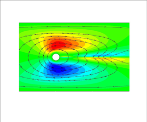
To understand the flow field of the new solution, we plot contours of the leading eigenvector of the ${u_x}$ velocity in figure 5(a) at $W{i_c} = 20.5$. Each component of the eigenvector is scaled with the L2-norm of the total vector. The eigenvector is positive at the upper gap and negative at the bottom gap between the cylinder and the wall. Hence, the velocity (and thus the flow rate) tends to increase at the upper gap, and this implies that more fluid passes from there. This is also evident from the streamlines of the perturbation solution which are shown with black lines and arrows. Of course, the sign of the eigenvector is arbitrary and the opposite configuration (of increasing velocity at the lower gap) is equally probable. However, the anti-symmetry of the eigenvector with respect to $y = 0$ will always lead to the asymmetric flow field.

Figure 5.

(a) Contours of the leading eigenvector of the ${u_x}$ velocity. (b) Contours of the superimposed solution of the ${u_x}$ velocity (2.10). (c) Contours of the leading eigenvector of the ${\tau _{xx}}$ stress component. (d) Contours of the superimposed solution of the ${\tau _{xx}}$ stress component (2.10) The properties of the material are $\varepsilon = 0.05, \beta = 0.05$. The blockage ratio is ${B_R} = 0.1$ and $Wi = 20.5$.

In figure 5(b), we plot contours of the ${u_x}$ velocity, which is a superposition of the base and the perturbed solution (see (2.10)). The contours correspond to a large dimensionless time $t = 20\;000$, so that we allow the perturbation to evolve significantly. We observe the desired result of flow asymmetry with respect to the y-axis, which resembles the result of Varchanis et al. (Reference Varchanis, Hopkins, Shen, Tsamopoulos and Haward2020a). We should note that the obtained flow profile is not identical with the results reported by Varchanis et al. (Reference Varchanis, Hopkins, Shen, Tsamopoulos and Haward2020a) because linear stability analysis provides information only about the onset and not the evolution of the instability.

The dominant term of the leading eigenvector is the ${\tau _{xx}}$ stress component (more than one order of magnitude larger than the velocity), which we plot in figure 5(c). The perturbed ${\tau _{xx,d}}$ component is also antisymmetric with respect to $y = 0$ and this causes the elastic birefringent strand to deviate from $y = 0$. This result is visualized in figure 5(d), where we plot the superimposed ${\tau _{xx}}$ component (see (2.10)), as we did for the velocity at $t = 20\;000$. The strand is distorted and the stress field becomes asymmetric at the wake of the cylinder. Similar results about the principle stress difference (PSD) are reported in the work by Varchanis et al. (Reference Varchanis, Hopkins, Shen, Tsamopoulos and Haward2020a).

To provide insight into the mechanism of the instability, we perform an energy analysis similar to previous works (Joo & Shaqfeh Reference Joo and Shaqfeh1991, Reference Joo and Shaqfeh1992; Byars et al. Reference Byars, Öztekin, Brown and McKinley1994; Ganpule & Khomami Reference Ganpule and Khomami1999; Grillet et al. Reference Grillet, Bogaerds, Peters and Baaijens2002; Smith et al. Reference Smith, Joo, Armstrong and Brown2003; Karapetsas & Tsamopoulos Reference Karapetsas and Tsamopoulos2013; Pettas et al. Reference Pettas, Karapetsas, Dimakopoulos and Tsamopoulos2015, Reference Pettas, Karapetsas, Dimakopoulos and Tsamopoulos2019). To this end, we take the inner product of the linearized momentum equation (i.e. (2.11)) with the perturbed velocity vector ${\boldsymbol{u}_p}$. Combining equations (2.11) and (2.13), we obtain an expression for the rate of change of the perturbed polymeric energy of the system, $\textrm{d}{E_p}/\textrm{d}t$, which is a combination of purely elastic energy production, $\textrm{d}{E_{el}}/\textrm{d}t$, and purely viscous dissipation, $\textrm{d}VD/\textrm{d}t$, of the material:

(4.1)

\begin{equation}\frac{{\textrm{d}{E_{el}}}}{{\textrm{d}t}} = \frac{{\textrm{d}VD}}{{\textrm{d}t}} + {\varphi _{pr}} + {\varphi _{p{s_1}}} + {\varphi _{p{u_1}}} + {\varphi _{p{s_2}}} + {\varphi _{p{u_2}}} + {\varphi _{rel}} + {\varphi _{vis}}.\end{equation}

The term $\textrm{d}{E_{el}}/\textrm{d}t$ indicates the onset of instability when it becomes positive so that when the perturbation grows in time, more elastic energy is stored. The definitions of all functionals and the methodology for obtaining (4.1) are analysed in Appendix C. In figure 6, we plot each term against the Weissenberg number. As expected, $\textrm{d}{E_{el}}/\textrm{d}t$ becomes positive at $W{i_c} = 20.5$. As a result of the increasing energy of the system, more energy can be dissipated by the viscous component so that $\textrm{d}VD/\textrm{d}t$ also increases. However, the two terms are not equal and their difference, i.e. $\textrm{d}{E_p}/\textrm{d}t$, remains positive for $Wi > W{i_c}$. For visualization purposes, we plot $\textrm{d}{E_{el}}/\textrm{d}t$ instead of $\textrm{d}{E_p}/\textrm{d}t$ as an indicator of instability, because it is much clearer when it becomes positive and how it increases with $Wi$ in the scale of figure 6.

Figure 6.

Energy terms (4.1) against $Wi$. The properties of the material are $\varepsilon = 0.05,\;\beta = 0.05$. The blockage ratio is ${B_R} = 0.1$.

The positive terms on the right-hand side of (4.1) are responsible for the onset of the instability (excluding $\textrm{d}VD/\textrm{d}t$):

(4.2a)

\begin{gather}{\varphi _{ps1}} ={-} \int {\left[ {\boldsymbol{\nabla }\boldsymbol{\cdot }\left( {\frac{{Wi}}{{{f_b}}}{\boldsymbol{u}_b}\boldsymbol{\cdot }\boldsymbol{\nabla }{\boldsymbol{\tau }_p}} \right)} \right]\boldsymbol{\cdot }{\boldsymbol{u}_p}\,\textrm{d}V} ,\end{gather}

(4.2b)

\begin{gather}{\varphi _{pu2}} = \int {\left\{ {\boldsymbol{\nabla }\boldsymbol{\cdot }\left[ {\frac{{Wi}}{{{f_b}}}(\boldsymbol{\nabla }\boldsymbol{u}_P^T\boldsymbol{\cdot }{\boldsymbol{\tau }_b} + {\boldsymbol{\tau }_b}\boldsymbol{\cdot }\boldsymbol{\nabla }{\boldsymbol{u}_p})} \right]} \right\}\boldsymbol{\cdot }{\boldsymbol{u}_p}\,\textrm{d}V} ,\end{gather}

(4.2c)

\begin{gather}{\varphi _{rel}} ={-} \int {\left[ {\boldsymbol{\nabla }\boldsymbol{\cdot }\left( {\frac{{{f_p}}}{{{f_b}}}{\boldsymbol{\tau }_b}} \right)} \right]\boldsymbol{\cdot }{\boldsymbol{u}_p}\,\textrm{d}V.} \end{gather}

All three terms arise from the constitutive model indicating that the instability is caused by the viscoelastic nature of the material. The second term, ${\varphi _{pu2}}$, is a coupling between base stresses and velocity gradient perturbations. It is physically related to material extensibility (the upper convected derivative terms introduce normal stresses in shear flows). The third term is derived from perturbations of the viscoelastic function, f, which in turn affect the effective material properties (polymeric viscosity and relaxation time). The first and most dominant term, ${\varphi _{ps1}}$, is a combination of base velocity and stress gradient perturbations. It is noteworthy that this term is negligible in commonly observed elastic instabilities, such as those in Taylor–Couette and Taylor–Dean geometries (Joo & Shaqfeh Reference Joo and Shaqfeh1992). Here, ${\varphi _{ps1}}$ is related to the convection of the viscoelastic stresses. As discussed by Varchanis & Tsamopoulos (Reference Varchanis and Tsamopoulos2022) and Yokokoji et al. (Reference Yokokoji, Varchanis, Shen and Haward2023), when a fluid parcel moves along a curved streamline, the convection of viscoelastic stresses causes the stress and strain rate to vary out of phase locally. The two quantities are not in equilibrium for some time which is proportional to the relaxation time, i.e. the time that is required for the material to adapt to the change. This lag creates an apparent shear-thinning effect in the flow past a confined cylinder. Thus, ${\varphi _{ps1}}$ can be seen as a measure of apparent viscoelastic thinning effects. According to this analysis, we also expect non-shear thinning fluid models (e.g. Oldroyd-B or FENE-CR) to exhibit steady asymmetric flow states as long as the value of the viscosity ratio $\beta $ is small (since $\beta $ is also related to the relaxation time ${\tilde{\lambda }_{rel}} = {\tilde{\eta }_p}/\tilde{G} = \tilde{\eta }(1 - \beta )/\tilde{G}$ which quantifies the apparent shear-thinning effect). At low $\beta $ values, variations in the flow resistance at the two sides of the cylinder can be significant in regions where the apparent shear-thinning effect is important, i.e. where strain rate changes are abrupt, and the stress must vary considerably to reach its new appropriate value. However, high $\beta $ values suppress any variations in flow resistance at the sides of the cylinder and only lead to symmetric steady states. This will be examined further in § 4.4. It should be noted that Boger fluids in experiments are usually characterized by large $\beta $, so the 2-D instability will be absent in these cases.

Moreover, we are interested in identifying the region around the cylinder where the instability arises. Thus, we also evaluate the terms of (4.1) at the two important parts of the domain: (a) at the upper gap between the cylinder and the channel wall (for $|x|< y \le H \textrm{and}\;{x^2} + {y^2} \ge 1$); and (b) close to the rear stagnation point $(|y|< x < 10R,\;{x^2} + {y^2} \ge 1)$. We plot the results in figure 7. In figure 7(a), we note that the terms at the gap between the cylinder and the wall are an order of magnitude smaller $(O({10^{ - 6}}))$ compared with their values at the whole domain. However, in figure 7(b), we can see that the terms at the wake of the cylinder are those that contribute the most to the total result. Consequently, the instability is triggered at the rear stagnation point where large perturbations of tensile stresses at the wake (figure 5c) cause fluctuations in the strain rate. The continuous interplay between imbalanced stress and strain rate can be sustained when the material is shear-thinning, because the viscosity is continuously changing as well. The process goes on until fluctuations propagate at the cylinder-wall gaps, where the result of the instability (the lateral flow asymmetry) becomes evident.

Figure 7.

Energy terms (4.1) against $Wi$ evaluated at (a) $|x|< y \le H\;\textrm{and}\;{x^2} + {y^2} \ge 1$ (upper gap between the cylinder and the wall), (b) $|y|< x < 10R,\;{x^2} + {y^2} \ge 1$ (downstream region). The properties of the material are $\varepsilon = 0.05,\;\beta = 0.05$. The blockage ratio is ${B_R} = 0.1$.

4.2. L-PTT model: parametric study

4.2.1. The effect of the viscosity ratio, β

The effect of the solvent is examined by varying the solvent to total viscosity ratio $\beta $. In figure 8(a), we plot the real part of the leading eigenvalue against the Weissenberg number for $\varepsilon = 0.05,\;{B_R} = 0.1$ and three different values of $\beta $. In all three cases, the eigenvalue is negative at small $Wi$ and it becomes positive at the respective $W{i_c}$ as seen in table 2. After reaching a maximum ($\textrm{Re}({\lambda _{max}}) = 0.019$ for $\beta = 0.05, \textrm{Re}({\lambda _{max}}) = 2.7 \times {10^{ - 4}}$ for $\beta = 0.07$), it decreases and eventually becomes negative again at a second critical $Wi$, see table 2. The appearance of $W{i_{{c_2}}}$ is expected at very intense flow conditions (at large $Wi$), where the shear rate is so large that the shear-thinning effect becomes negligible (solvent shear stresses >> viscoelastic shear stresses) and steady states with different flow resistance at the sides of the cylinder cannot be supported. Thus, the flow re-symmetrizes, even though elasticity increases. Flow re-symmetrization has also been reported experimentally in the viscoelastic flow around a cylinder by Haward et al. (Reference Haward, Hopkins and Shen2020).

Figure 8.

(a) Real part of the leading eigenvalue versus $Wi$ for $\beta = 0.05$, black line with triangles; $\beta = 0.06$, red line with circles; $\beta = 0.07$, blue line with stars. (b) $W{i_c}$ and $W{i_{{c_2}}}$ against $\beta $. $W{i_c}$ by SV (Varchanis et al. Reference Varchanis, Hopkins, Shen, Tsamopoulos and Haward2020a), black triangles. Present work (linear stability, denoted as LS): $W{i_c}$, red line with circles; $W{i_{{c_2}}}$, blue line with stars. In all cases, $\varepsilon = 0.05,\;{B_R} = 0.1$.

Table 2.

$W{i_c}$ and $W{i_{{c_2}}}$ at each simulated $\beta $ case.

With increasing $\beta $, the (Newtonian) solvent contribution is amplified and shear-thinning is reduced. As a result, larger $Wi$ is required for non-Newtonian characteristics (elasticity and shear-thinning) to become significant. Thus, $W{i_c}$ increases with $\beta $, while the leading eigenvalue is smaller at fixed $Wi$. Moreover, the symmetric flow restabilizes at smaller $W{i_{{c_2}}}$. In figure 8(b), we plot $W{i_c}$ and $W{i_{{c_2}}}$ against $\beta $. Again, we observe that $W{i_c}$ increases with $\beta $, but $W{i_{{c_2}}}$ decreases. We compare our results with those by SV (Varchanis et al. Reference Varchanis, Hopkins, Shen, Tsamopoulos and Haward2020a). Varchanis et al. (Reference Varchanis, Hopkins, Shen, Tsamopoulos and Haward2020a) did not report $W{i_{{c_2}}}$, but regarding $W{i_c}$, our predictions match their numerical values. In the limit $\beta \to 0.075$, the two critical Weissenberg numbers merge and the instability is not triggered at all at higher viscosity ratios. Overall, for higher $\beta $, the asymmetric flow instability is observed for a smaller range of $Wi$ (or flow rate experimentally), because elasticity and shear-thinning are equally important only at limited flow conditions and instability is triggered when both are present.

Additionally, we determine the wall shear rate at the minimum gap width between the cylinder and the walls by a simple mass balance:

(4.3)

\begin{equation}{\widetilde {\dot{\gamma }}_{w,gap}} = \frac{{6{{\widetilde {\dot{\gamma }}}_{ch}}{B_R}}}{{{{(1 - {B_R})}^2}}}.\end{equation}

In figure 9, we plot in log-linear scale the flow curve (i.e. shear viscosity versus shear rate) for $\beta = 0.06$ and $\beta = 0.07$. We obtain these plots by solving the constitutive equation (2.3) under steady shear. Naturally, the curves are very similar. We also provide the shear viscosity at the critical values ${\widetilde {\dot{\gamma }}_{w,gap,c}}$ (black triangles) and ${\widetilde {\dot{\gamma }}_{w,gap,{c_2}}}$ (red circles) at which the instability arises and vanishes, respectively. In both cases, at ${\widetilde {\dot{\gamma }}_{w,gap,c}}$, the viscosity decreases with the shear rate, but at ${\widetilde {\dot{\gamma }}_{{{w,gap,c}}_2}}$, the slope of the flow curve is significantly reduced. As noted before, shear-thinning is weak at this flow rate and the instability vanishes. Moreover, with increasing $\beta $, the two critical values of ${\widetilde {\dot{\gamma }}_{w,gap}}$ come closer, so that the symmetric flow is unstable at more limited conditions.

Figure 9.

Viscosity versus shear rate in log-linear plot. Predictions of the L-PTT model for $\varepsilon = 0.05$: $\beta = 0.06$ (blue line) and $\beta = 0.07$ (pink dashed line). Critical shear rate for the onset of the instability, ${\widetilde {\dot{\gamma }}_{w,gap,c}}$ (black triangles), and critical shear rate for re-stabilization, ${\widetilde {\dot{\gamma }}_{w,gap,{c_2}}}$ (red circles), for each case.

4.2.2. The effect of the extensibility parameter $\varepsilon $

The effect of elasticity is examined by varying the extensibility parameter $\varepsilon $. In the limit $\varepsilon \to 0$, the L-PTT model reduces to the Oldroyd-B model in which the macromolecular chains are infinitely extensible. In figure 10(a), we plot the real part of the leading eigenvalue against $Wi$ for $\beta = 0.05,\;{B_R} = 0.1$ and three different values of $\varepsilon $. The predictions are similar to those of increasing $\beta $. With increasing $\varepsilon $, the material is less extensible and more shear-thinning. It is only at large $Wi$ that elasticity introduces sufficient fluctuations at the rear pole of the cylinder. Thus, $W{i_c}$ increases. For larger $\varepsilon $, the leading eigenvalue is smaller and the symmetric flow is restabilized at smaller $W{i_{{c_2}}}$, see table 3. In figure 10(b), we plot $W{i_c}$ and $W{i_{{c_2}}}$ against $\varepsilon $. Here, $W{i_c}$ increases with $\varepsilon $, but $W{i_{{c_2}}}$ decreases so that the range of flow rates for which the instability is observed is smaller. Again, our results for $W{i_c}$ agree with SV (Varchanis et al. Reference Varchanis, Hopkins, Shen, Tsamopoulos and Haward2020a). In the limit $\varepsilon \to 0.09$ and beyond, elasticity is weak at small $Wi$, and it cannot contribute as required to generate the instability. For the same $\varepsilon $, at larger $Wi$ where elasticity is important, shear-thinning is weak, and their combined effect cannot induce the elastic instability. Thus, no flow asymmetry is observed.

Figure 10.

(a) Real part of the leading eigenvalue versus $Wi$ for $\varepsilon = 0.05$, black line with triangles; $\varepsilon = 0.07$, red line with circles; $\varepsilon = 0.08$, blue line with stars. (b) $W{i_c}$ and $W{i_{{c_2}}}$ against $\varepsilon $. $W{i_c}$ by SV (Varchanis et al. Reference Varchanis, Hopkins, Shen, Tsamopoulos and Haward2020a), black triangles. Present work (LS): $W{i_c}$, red line with circles; $W{i_{{c_2}}}$, blue line with stars. In both cases, $\beta = 0.05,\;{B_R} = 0.1$.

Table 3.

$W{i_c}$ and $W{i_{{c_2}}}$ at each simulated $\varepsilon $ case.

We refer to the flow curve again (figure 11) to justify the interplay between elasticity and shear-thinning. We show the predictions of the L-PTT model for $\varepsilon = 0.07$ and $\varepsilon = 0.085$, along with the critical values of the shear rate as in figure 9. We note again that the value of ${\widetilde {\dot{\gamma }}_{w,gap,{c_2}}}$ is such that the slope of the flow curve is small and shear-thinning is weak. With increasing $\varepsilon $, the critical shear rates tend to merge, and, in this case, the instability cannot be triggered at all.

Figure 11.

Viscosity versus shear rate in log-linear plot. Predictions of the L-PTT model for $\beta = 0.05$, $\varepsilon = 0.07$ (blue line) and $\varepsilon = 0.085$ (pink dashed line). ${\widetilde {\dot{\gamma }}_{w,gap,c}}$ (black triangles) and ${\widetilde {\dot{\gamma }}_{w,gap,{c_2}}}$ (red circles) for each case.

4.2.3. The effect of the confinement ${B_R} = R/H$

We investigate the effect of the geometry through the blockage ratio ${B_R}$. By decreasing the height of the channel H, ${B_R}$ increases and the flow becomes more confined between the cylinder and the plates increasing locally the shear rate and the extension rate at the rear stagnation point. In figure 12(a), we report $\textrm{Re}(\lambda )$ against $Wi$ for three different ${B_R}$. The material properties are $\beta = 0.05,\;\varepsilon = 0.05$. For larger ${B_R}$, the leading eigenvalue increases more abruptly and $W{i_c}$ is smaller. The leading eigenvalue also decreases faster after reaching a maximum so that $W{i_{{c_2}}}$ is smaller too, see table 4. In figure 12(b), we plot $W{i_c}$ and $W{i_{{c_2}}}$ against ${B_R}$, and we observe the same behaviour: both $W{i_c}$ and $W{i_{{c_2}}}$ and the range of flow rates leading to asymmetric fluxes decrease with ${B_R}$. Our results for both critical $Wi$ agree with SV (Varchanis et al. Reference Varchanis, Hopkins, Shen, Tsamopoulos and Haward2020a).

Figure 12.

(a) Real part of the leading eigenvalue versus $Wi$ for ${B_R} = 0.10$, red line with circles; ${B_R} = 0.15$, black line with triangles; ${B_R} = 0.20$, blue line with stars. (b) $W{i_c}$ and $W{i_{{c_2}}}$ against ${B_R}$. SV (Varchanis et al. Reference Varchanis, Hopkins, Shen, Tsamopoulos and Haward2020a): $W{i_c}$, black triangles; $W{i_{{c_2}}}$, green squares. Present work (LS): $W{i_c}$, red line with circles; $W{i_{{c_2}}}$, blue line with stars. The material properties are $\varepsilon = 0.05,\;\beta = 0.05$.

Table 4.

$W{i_c}$ and $W{i_{{c_2}}}$ at each simulated ${B_R}$ case.

In contrast to the cases of $\beta $ and $\varepsilon $, $W{i_c}$ decreases with ${B_R}$. From (4.3), the wall shear rate at the minimum gap between the cylinder and the wall increases with ${B_R}$, even though the critical characteristic shear rate decreases $({\widetilde {\dot{\gamma }}_{ch,c}} = W{i_c}/{\tilde{\lambda }_{rel}})$. As a result, shear-thinning is more intense at the gap when the flow is more confined and the instability is triggered earlier. In figure 12(b), we note that for ${B_R} = 0.25$, the critical $Wi$ increases slightly. In such confined flow conditions, shear-thinning is intense at small $Wi$, while elasticity is still weak. A slight increase of $Wi$ results in higher elasticity, while the slope of the flow curve decreases (see figure 13). Thus, there is a point beyond which elasticity produces sufficient fluctuations, and, simultaneously, the shear viscosity is effectively affected by these fluctuations. At even higher ${B_R}$, the perturbations are confined at the rear stagnation point. Then, even when elasticity is very important, shear-thinning is not because the shear rate is very large. As a result, the flow resistance and, consequently, the lateral asymmetry is minimal and the instability is absent.

Figure 13.

Viscosity versus shear rate in log-linear plot. Predictions of the L-PTT model for $\beta = 0.05, \varepsilon = 0.05$ (blue line). ${\widetilde {\dot{\gamma }}_{w,gap,c}}$ (black triangles) and ${\widetilde {\dot{\gamma }}_{w,gap,{c_2}}}$ (red circles) for every simulated ${B_R}$ case.

In figure 13, we plot in log-linear scale the flow curve of the L-PTT model for $\beta = 0.05,\;\varepsilon = 0.05$. With symbols, we denote ${\widetilde {\dot{\gamma }}_{w,gap,c}}$ (at the onset of the instability) and ${\widetilde {\dot{\gamma }}_{w,gap,{c_2}}}$ (at flow re-symmetrization) for every case of ${B_R}$. Therefore, when the instability is triggered (black triangles), the material is shear-thinning. However, the flow becomes symmetric again (red circles) when shear-thinning is not so strong. Qualitatively, the slope at the onset of the instability varies from $- 0.06$ to $- 0.034$, while at flow re-symmetrization, it is three times smaller in magnitude and ranges from $- 0.018$ to $- 0.013$.

4.3. L-PTT model: Dependence of $W{i_c}$ and $W{i_{c2}}$ on material properties and geometry

In this section, we provide simple formulae to estimate the conditions under which the instability arises. First, we provide an expression for $W{i_c}$ in terms of the material properties and the level of confinement. From figures 8(b), 10(b) and 12(b), we observe that $W{i_c}$ depends exponentially on $\beta ,\varepsilon $ and ${B_R}$. Thus, we propose the following expression:

(4.4)

\begin{equation}W{i_c} = {\textrm{e}^{({c_1}\beta + {c_2}\varepsilon + {c_3}{B_R})}} + {c_4},\end{equation}

where ${c_1},{c_2},{c_3}$ are the coefficients that measure the importance of $\beta ,\varepsilon $ and ${B_R}$, respectively, on $W{i_c}$. The coefficients are evaluated through nonlinear regression on the data points which we have already obtained through linear stability analysis. The values are summarized in table 5.

Table 5.

Values of coefficients of (4.4), obtained through nonlinear regression.

In figure 14, we present the predictions of (4.4) against the results from linear stability analysis. The agreement is excellent except for very small $\varepsilon $ (figure 14b), where shear-thinning is negligible at a large range of shear rates. Note that the equation is accurate for the L-PTT model, but its purpose is to provide a quick estimate for the critical conditions and not accurate values especially outside of the ranges that have been examined here. For other constitutive equations, similar expressions can be defined and tested against numerical and experimental results.

Figure 14.

$W{i_c}$ against: (a) $\beta $; (b) $\varepsilon $; (c) ${B_R}$. Predictions of (4.4) (black line, Fit) and results from linear stability analysis (red symbols, LS).

We follow a similar approach for the second critical Weissenberg number. In this case, a linear expression is more appropriate:

(4.5)

\begin{equation}W{i_{{c_2}}} ={-} {c_1}\beta - {c_2}\varepsilon - {c_3}{B_R} + {c_4}.\end{equation}

Again, ${c_1},{c_2},{c_3}$ are the coefficients that measure the importance of $\beta ,\varepsilon $ and ${B_R}$, respectively, on $W{i_{{c_2}}}$. Through nonlinear regression, we obtain the values of the coefficients (table 6).

Table 6.

Values of coefficients of (4.5), obtained through nonlinear regression.

The predictions of (4.5) nicely fit the numerical values of linear stability (figure 15).

Figure 15.

$W{i_{{c_2}}}$ against: (a) $\beta $; (b) $\varepsilon $; (c) ${B_R}$. Predictions of (4.5) (black line, Fit) and results from linear stability analysis (blue symbols, LS).

Next, we examine the predictions of the linear stability analysis against the criterion for elastic instabilities proposed by McKinley et al. (Reference McKinley, Pakdel and Öztekin1996) and Pakdel & McKinley (Reference Pakdel and McKinley1996). These authors argue that the combination of elastic extensional stresses along a streamline and the curvature of these streamlines can extend a macromolecular chain asymmetrically between streamlines. This is also affected by the intensity of the shearing part of the flow. In the case of the cylinder, at the rear stagnation point, where the streamlines are curved and material undergoes large extension, a perturbation of the stress field is likely to occur. This alters the local shear rate and, due to the shear thinning nature of the material, the shear viscosity is affected. Under certain conditions, when shear thinning is strong enough, the perturbation can grow and cause a global flow instability, in which local variations in the flow resistance propagate to the rest of the domain. The authors’ criterion finally involves an interplay between normal stresses and curved streamlines:

(4.6)

\begin{equation}{\left( {\frac{{{{\tilde{\lambda }}_{rel}}\tilde{U}}}{{{{\tilde{R}}_c}}}\frac{{{{\tilde{\tau }}_{xx}}}}{{{{\tilde{\eta }}_0}{{\widetilde {\dot{\gamma }}}_{Rc}}}}} \right)^{1/2}} \ge {M_c}.\end{equation}

Here, ${\tilde{R}_c}$ is the radius of curvature of the streamlines, ${\tilde{\eta }_0}$ is the zero-shear-rate viscosity and ${\widetilde {\dot{\gamma }}_{Rc}} = \tilde{U}/{\tilde{R}_c}$ is a characteristic local deformation rate. Additionally, ${M_c}$ is a critical value which must be surpassed so that local fluctuations grow and the instability is triggered. Following the authors’ suggestion (McKinley et al. Reference McKinley, Pakdel and Öztekin1996), we can describe ${\tilde{R}_c}$ as a function of the height of the channel and the radius of the cylinder:

(4.7)

\begin{equation}\frac{1}{{{{\tilde{R}}_c}}} = \frac{a}{{\tilde{R}}} + \frac{b}{{\tilde{H}}} = \frac{1}{{\tilde{R}}}(a + b{B_R}).\end{equation}

Here, a and b are constants which characterize the sensitivity of the curvature of the streamlines to the geometrical aspect ratio. We can define the zero-rate relaxation time, ${\tilde{\lambda }_{rel,0}}$, and the zero-rate first normal stress coefficient ${\tilde{\varPsi }_{1,0}} = 2(1 - \beta ){\tilde{\eta }_0}{\tilde{\lambda }_{rel,0}}$. For a more precise description of the criterion, we must take into account that the material properties are strain-rate dependent, so that ${\tilde{\lambda }_{rel}}(\widetilde {\dot{\gamma }}) = {\tilde{\varPsi }_1}(\widetilde {\dot{\gamma }})/2{\tilde{\eta }_p}(\widetilde {\dot{\gamma }})$ and ${\tilde{\varPsi }_1}(\widetilde {\dot{\gamma }}) = {\tilde{\tau }_{xx}}(\widetilde {\dot{\gamma }})/{\widetilde {\dot{\gamma }}^2}$ (${\tilde{\tau }_{yy}} = 0$ in the L-PTT model). Considering all the above, and that $Wi = {\tilde{\lambda }_{rel,0}}\tilde{U}/\tilde{R}$, the criterion becomes

(4.8)

\begin{equation}\begin{array}{ccccc} & {\left( {\dfrac{{{{\tilde{\lambda }}_{rel}}\tilde{U}}}{{\tilde{R}}}(a + b{B_R}){{\widetilde {\dot{\gamma }}}_{Rc}}\dfrac{{{{\tilde{\varPsi }}_1}}}{{{{\tilde{\eta }}_0}}}\dfrac{{{{\tilde{\varPsi }}_{1,0}}}}{{{{\tilde{\varPsi }}_{1,0}}}}} \right)^{1/2}} \ge {M_c}\\ & \quad \to {\left( {Wi(a + b{B_R})\dfrac{{{{\tilde{\lambda }}_{rel}}}}{{{{\tilde{\lambda }}_{rel,0}}}}Wi(a + b{B_R})\dfrac{{{{\tilde{\varPsi }}_1}2(1 - \beta )}}{{{{\tilde{\varPsi }}_{1,0}}}}\; } \right)^{1/2}} \ge {M_c}\\ & \quad \to Wi(a + b{B_R}){\left( {\dfrac{{{{\tilde{\lambda }}_{rel}}}}{{{{\tilde{\lambda }}_{rel,0}}}}\dfrac{{{{\tilde{\varPsi }}_1}}}{{{{\tilde{\varPsi }}_{1,0}}}}2(1 - \beta )} \right)^{1/2}} \ge {M_c}. \end{array}\end{equation}

This can be reformulated at the critical conditions to

(4.9a)

\begin{gather}\frac{1}{{W{i_c}}} = a^{\prime} + b^{\prime}{B_R},\end{gather}

(4.9b)

\begin{gather}a^{\prime} = \frac{{a\sqrt {2(1 - \beta )} }}{{{M^{\prime}_c}}},\end{gather}

(4.9c)

\begin{gather}b^{\prime} = \frac{{b\sqrt {2(1 - \beta )} }}{{{M^{\prime}_c}}},\end{gather}

(4.9d)

\begin{gather}{M^{\prime}_c} = {M_c}{\left[ {\frac{{{{\tilde{\varPsi }}_{1,0}}}}{{{{\tilde{\varPsi }}_1}({{\widetilde {\dot{\gamma }}}_{Rc}})}}\frac{{{{\tilde{\lambda }}_{rel,0}}}}{{{{\tilde{\lambda }}_{rel}}({{\widetilde {\dot{\gamma }}}_{Rc}})}}} \right]^{1/2}}.\end{gather}

In figure 16, we plot the inverse of $W{i_c}$ against ${B_R}$. We note that the points can indeed be approximated by a line, but nonlinearities arise for ${B_R} > 0.2$. This happens because $W{i_c}$ slightly increases at ${B_R} = 0.25$ (see discussion in § 4.2.3). By fitting the linear regime, we find $a^{\prime}=1.48\times 10^{-3}$ and $b^{\prime} = 0.437$.

Figure 16.

$1/W{i_c}$ against ${B_R}$. Numerical results (black triangles) and linear fitting (red line).

We can scale (4.7) by setting $a = 1$. In our case, the viscosity ratio is $\beta = 0.05$ and we find ${M^{\prime}_c} = 928.5$ (see (4.9b)) and $b = 294.2$ (see (4.9c)). Finally, we can calculate the local deformation rate for each ${B_R}$ and ${M_c}$ through (4.9d). To do this, we need the values of the material properties, ${\tilde{\varPsi }_1}({\widetilde {\dot{\gamma }}_{Rc}})$ and ${\tilde{\lambda }_{rel}}({\widetilde {\dot{\gamma }}_{Rc}})$, which can be calculated numerically or analytically (Alves, Pinho & Oliveira Reference Alves, Pinho and Oliveira2001b) from the steady shear predictions of the L-PTT model. We report the results in table 7. Here, ${M_c}$ increases with ${B_R}$, it reaches a maximum at ${B_R} = 0.1$ and then decreases again. The opposite is true for ${\widetilde {\dot{\gamma }}_{Rc}}$. In this way, we know the critical value for instability as a function of the geometry and the flow conditions of the problem.

Table 7.

Local deformation rate and the critical value for instability at a given ${B_R}$.

Local evaluation of the Pakdel–McKinley criterion can also be insightful in understanding the regions which are sensitive to elastic instabilities. Calculation of the local parameter $M_c^\ast $ has been performed previously by Cruz et al. (Reference Cruz, Poole, Afonso, Pinho, Oliveira and Alves2016) and particularly for the flow around a cylinder by Peng et al. (Reference Peng, Tang, Li, Zhang and Yu2023). Following these works, we define the dimensionless local Pakdel–McKinley parameter as a function of locally calculated quantities:

(4.10)

\begin{equation}\begin{array}{*{20}{c}} {M_c^\ast{=} {{\left( {\dfrac{{Wi|\boldsymbol{u}|}}{{{R_{c,loc}}}}\dfrac{{{\tau_{ss}}}}{{|\boldsymbol{\tau }{|_F}}}} \right)}^{1/2}},} \end{array}\end{equation}

where $|\boldsymbol{u}|$ is the velocity magnitude, ${R_{c,loc}} = |\boldsymbol{u}{|^3}/|\boldsymbol{u}\; \times (\textrm{D}\boldsymbol{u}/\textrm{D}t)|$ is the radius of curvature, ${\tau _{ss}} = {\boldsymbol{u}^T}\boldsymbol{\cdot }\boldsymbol{\tau }\boldsymbol{\cdot }\boldsymbol{u}/|\boldsymbol{u}{|^2}$ is the tensile stress in the streamwise direction and $|\boldsymbol{\tau }{|_F}$ is the Frobenius norm of the stress tensor. In figure 17, we present contours of $M_c^\ast $ at the region around the cylinder for the main case $(\beta = 0.05,\;\varepsilon = 0.05,\;{B_R} = 0.1)$, at $Wi = 20.5$, beyond the critical conditions. The quantities are calculated using the base solution. The parameter is large at the cylinder-wall gaps, due to the small radius of curvature of the streamlines. However, its largest values are located close to the rear stagnation point, because of the large shear and tensile stresses, as well as the small radius of curvature. Clearly, both regions are prone to instability, but, as suggested by the energy analysis, the perturbations are more pronounced at the stagnation point and the instability will be triggered there.

Figure 17.

Contours of the Pakdel–McKinley parameter around the cylinder. The material and geometric parameters are $\beta = 0.05,\;\varepsilon = 0.05,\;{B_R} = 0.1$ and $Wi = 20.5$.

4.4. Predictions of the m-L-PTT model: is a shear-thinning flow curve necessary?

In § 4.1, we revealed the energy terms that contribute to the instability, stating that the convection of the viscoelastic stresses is the most important one. This term creates an apparent shear-thinning effect because it forces the stresses to vary out of phase with the strain rate. Any seemingly non-shear-thinning model predicts this behaviour, despite predicting constant shear viscosity in simple shear, because the material derivative term is absent in this ideal flow. Because of this, we expect the asymmetric flow instability to arise under conditions where this apparent shear-thinning term is significant, i.e. when the solvent contribution is minimal. To test this hypothesis, we repeat the analysis, this time using the modified L-PTT model (m-L-PTT) (Coates, Armstrong & Brown Reference Coates, Armstrong and Brown1992; Oliveira Reference Oliveira2009). The governing equations are the same, except for (2.3) being replaced with (2.7). The predictions of the model in viscometric flows are similar to L-PTT, but the shear viscosity is constant in simple shear; see Appendix A. We examine the effect of the viscosity ratio $\beta $ for $\varepsilon = 0.05$ and ${B_R} = 0.1$. For small $\beta $, the model indeed predicts the asymmetric flow instability, but at larger $W{i_c}$ (figure 18). For example, for $\beta = 0$, $W{i_c} = 19.0$, while in the case of the L-PTT model, $W{i_c} = 12.6$. This is an expected result because the shear-thinning response is not as strong as in the L-PTT case. Here, $W{i_c}$ increases abruptly with $\beta $ and the instability vanishes beyond $\beta \approx 0.025$ when the solvent severely affects the apparent shear-thinning response. For the same $\varepsilon $ and ${B_R}$, the L-PTT model can reproduce the instability up to $\beta \approx 0.075$. The eigenvector of the leading eigenvalue at the critical conditions is similar to that of figure 5. The dominant energy terms are also the same as in the L-PTT case. Thus, the instability is the same in nature, but it is limited by the weak apparent shear-thinning response of the material.

Figure 18.

$W{i_c}$ against $\beta $ using the m-L-PTT model. In all cases, $\varepsilon = 0.05,\; {B_R} = 0.1$.

Since the instability is triggered only for small $\beta $, it should not be observed in typical experiments involving Boger fluids, because their solvent viscosity is usually large. For example, McKinley et al. (Reference McKinley, Armstrong and Brown1993) report in Boger fluids a three-dimensional (3-D) periodic flow instability at the wake of the cylinder, but no 2-D asymmetric flow. However, if such an instability can be triggered at small $\beta $, then we expect this 3-D instability to arise at $W{i_c}\sim O(1)$, well before the 2-D asymmetric flow instability $(W{i_c}\sim O(10))$. If additionally, the 3-D instability can be sustained at large $Wi$, we might observe both instabilities simultaneously; all these need to be examined.

4.5. Predictions of the e-PTT model: the effect of extension-rate thinning

In the final part of this study, we examine the effect of extension-rate thinning by replacing the L-PTT with the e-PTT model. An e-PTT material is slightly more shear-thinning, but more importantly, less elastic compared with an L-PTT material with the same remaining properties. Because of extension-rate thinning, normal stresses at the wake of the cylinder are significantly smaller and decrease with $Wi$. Thus, we expect lateral asymmetry to occur only when $Wi$ is large enough so that the material is shear-thinning, but simultaneously small enough for elastic tensile stresses to be important. We test the e-PTT model at $\beta = 0.05$ and ${B_R} = 0.1$ for different $\varepsilon $. At small $\varepsilon $, the two models predict similar $W{i_c}$. However, as we described above, the instability conditions for the e-PTT model are limited and the instability vanishes for $\varepsilon > 0.02$. The material is not elastic enough and normal stresses at the wake of the cylinder are unable to produce significant local fluctuations. In figure 19, we plot the leading eigenvector of the ${u_x}$ velocity for $\varepsilon = 0.03$ at $Wi = 30$. Note that the perturbations are confined at the wake of the cylinder. There is a slight tendency for the fluid to pass preferably through the lower gap between the cylinder and the wall. However, the magnitude of the velocity there is very small and the flow asymmetry is very weak. For larger $\varepsilon $ or larger $Wi$, the eigenvector is even more confined at the rear stagnation point and no asymmetry is evident.

Figure 19.

Leading eigenvector of the ${u_x}$ velocity for $\beta = 0.05,\;\varepsilon = 0.03,\;{B_R} = 0.1$ at $Wi = 30$ for a fluid following the e-PTT constitutive model.

5. Conclusions

In this work, we investigated the 2-D stability of the flow of a viscoelastic fluid around a confined cylinder. We reproduced the elastic instability leading to lateral flow asymmetry by means of linear stability analysis. This instability requires a combination of elasticity and shear-thinning, and it causes more fluid to pass through either the upper or the lower gap between the cylinder and the channel walls. Either one of the two configurations is equally probable. The transition occurs through a supercritical pitchfork bifurcation to the new steady solution. We performed an energy analysis, and we concluded that the instability is induced by coupling the base velocity with stress gradient perturbations and the base stress with velocity gradient perturbations. These terms arise from the upper convected derivative terms of the constitutive equation, indicating an instability which is absent in inelastic fluids. A third term that contributes mildly to the instability is the perturbation of the viscoelastic function, f, which is translated to perturbations of the effective material properties. The main contribution to these terms comes from the rear stagnation point, and that is where the instability is initiated, because of large tensile stress perturbations there.

We performed parametric studies on the material properties $\beta ,\varepsilon $ and the blockage ratio ${B_R}$. Larger $\beta $ (more Newtonian contribution) delays the instability and the critical $Wi$ increases. The same holds true for larger $\varepsilon $ because the polymer chains are less extensible, and it is rare for them to cross streamlines. With increasing ${B_R}$, the shear rate at the gap between the cylinder and the walls increases for a given $Wi$ (or flow rate). Thus, shear-thinning becomes important at smaller $Wi$ and $W{i_c}$ decreases. In general, a certain level of shear-thinning and elasticity is necessary for flow asymmetry to arise. Our results for $W{i_c}$ agree with previous studies (Varchanis et al. Reference Varchanis, Hopkins, Shen, Tsamopoulos and Haward2020a) in all cases.

Moreover, beyond a limiting value of the parameters $(\beta ,\varepsilon ,{B_R})$, the instability is not observed at all because the interplay between elasticity and shear-thinning is not established. Thus, we extended this work by reporting a second critical Weissenberg number, $W{i_{{c_2}}}$, at which the symmetric flow is re-stabilized. This happens at large $Wi$ where the flow is very intense and the shear rate is so large that the shear viscosity does not practically decrease anymore. For lower $\beta $ or $\varepsilon $, the material is more elastic and it can compensate for weaker shear thinning so that $W{i_{{c_2}}}$ increases. Here, $W{i_{{c_2}}}$ increases with decreasing ${B_R}$ as well, because the shear rate at the gap increases more mildly with the flow rate and shear-thinning is relevant at a wider range of Weissenberg numbers.

Additionally, we provided simple expressions for the critical Weissenberg numbers in terms of the material parameters and the level of confinement. Here, $W{i_c}$ depends exponentially on the parameters $(\beta ,\varepsilon ,{B_R})$, while $W{i_{{c_2}}}$ decreases linearly with $(\beta ,\varepsilon ,{B_R})$. The predictions match the numerical values that we obtained from linear stability. Similar expressions can be formulated for other viscoelastic models in the future. Moreover, we discussed the elastic instability criterion developed by McKinley et al. (Reference McKinley, Pakdel and Öztekin1996). We reported the critical value ${M_c}$ for the onset of the instability, depending on the blockage ratio ${B_R}$. Furthermore, we calculated the M value using local quantities and we found that the wake of the cylinder is more prone to instability, thus verifying the energy analysis result.

It is important to note that shear-thinning is not present only in models that predict decreasing shear viscosity in simple shear flow. An apparent shear-thinning effect is generated by the material derivative of the viscoelastic stresses even in models that are considered non-shear-thinning (Varchanis & Tsamopoulos Reference Varchanis and Tsamopoulos2022). Thus, these models can also predict asymmetric flows around a cylinder, though at limited flow conditions. We verified this statement with the modified L-PTT model which replicates a Boger fluid in simple shear. The instability arises at larger $W{i_c}$ and quickly vanishes with increasing $\beta $, because the apparent thinning effect is relatively weak and very sensitive to the contribution of the solvent.

Finally, we examined the predictions of the e-PTT model to assess the effect of extension-rate thinning. For small $\varepsilon $, both models predict similar results. With increasing $\varepsilon $, the instability vanishes in an e-PTT fluid, because tensile stresses at the rear of the cylinder decrease abruptly with $Wi$. At flow conditions where the shear viscosity decreases, elastic stresses are not strong enough to produce fluctuations at the wake of the cylinder. Thus, elasticity and shear-thinning cannot effectively interact, and the asymmetry in the flow is minimal.

In the future, we would like to extend this work to other elastic instabilities in the flow around a confined cylinder, such as those that arise due to the presence of inertia (Kenney et al. Reference Kenney, Poper, Chapagain and Christopher2013; Shi et al. Reference Shi, Kenney, Chapagain and Christopher2015) or more complex 3-D structures (McKinley et al. Reference McKinley, Armstrong and Brown1993). Additionally, it would be interesting to examine more complex and practical geometries such as arrays of cylinders (Smith et al. Reference Smith, Joo, Armstrong and Brown2003; Shi & Christopher Reference Shi and Christopher2016) or even instabilities in porous media (Kawale et al. Reference Kawale, Marques, Zitha, Kreutzer, Rossen and Boukany2017; Carlson et al. Reference Carlson, Toda-Peters, Shen, Haward, Carlson, Toda-Peters, Shen and Haward2022; Browne et al. Reference Browne, Huang, Zheng and Datta2023).

Funding

The research work was supported by the Hellenic Foundation for Research and Innovation (HFRI) under the Project ‘MOFLOWMAT’ (HFRI-FM17-2309), P.M. was supported by HFRI under the 3rd Call for HFRI PhD Fellowships (fellowship number 5854) and Y.D. was supported by HFRI under the Project ‘CARE’ (HFRI-FM17-876).

Declaration of interests

The authors report no conflict of interest.

Appendix A. Model predictions in viscometric flows

The predictions of the three viscoelastic models in steady shear and uniaxial elongation are presented in figure 20. The material parameters are $\beta = 0.05,\;\varepsilon = 0.05$ and ${\tilde{\lambda }_{rel}} = 0.145\;\textrm{s}$. In steady shear (figure 20a), the L-PTT and e-PTT models offer similar shear-thinning response, while the m-L-PTT predicts constant shear viscosity. However, the e-PTT model predicts extension rate hardening and then extensional rate thinning at large extension rate (figure 20b). The L-PTT and m-L-PTT models predict extension rate hardening and constant extensional viscosity at large $\dot{\varepsilon }$.

Figure 20.

(a) Shear viscosity in steady shear flow, (b) extensional viscosity in steady uniaxial flow. Predictions of the three models: L-PTT (black), m-L-PTT (red), e-PTT (blue). The material parameters are $\beta = 0.05,\;\varepsilon = 0.05$ and ${\tilde{\lambda }_{rel}} = 0.145\;\textrm{s}$.

Appendix B. Details of the equations

B.1. Strong form of the linearized equations

Equations (2.11)–(2.13) read in detail:

(B1)

\begin{equation}- \boldsymbol{\nabla }{P_p} + \boldsymbol{\nabla }\boldsymbol{\cdot }{\boldsymbol{\tau }_p} + \beta \boldsymbol{\nabla }\boldsymbol{\cdot }{\dot{\boldsymbol{\gamma }}_p} = {\bf 0},\end{equation}

with ${\dot{\boldsymbol{\gamma }}_p} = \boldsymbol{\nabla }{\boldsymbol{u}_p} + \boldsymbol{\nabla }\boldsymbol{u}_p^T$.

(B2)

\begin{gather}\boldsymbol{\nabla }\boldsymbol{\cdot }{\boldsymbol{u}_p} = 0,\end{gather}

(B3)

\begin{gather}\begin{array}{@{}l@{}} \displaystyle Wi[\lambda {\boldsymbol{\tau }_p} + {\boldsymbol{u}_b}\boldsymbol{\cdot }\boldsymbol{\nabla }{\boldsymbol{\tau }_p} + {\boldsymbol{u}_p}\boldsymbol{\cdot }\boldsymbol{\nabla }{\boldsymbol{\tau }_b} - \boldsymbol{\nabla }\boldsymbol{u}_b^T\boldsymbol{\cdot }{\boldsymbol{\tau }_p} - \boldsymbol{\nabla }\boldsymbol{u}_p^T\boldsymbol{\cdot }{\boldsymbol{\tau }_b} - \; {\boldsymbol{\tau }_b}\boldsymbol{\cdot }\boldsymbol{\nabla }{\boldsymbol{u}_p} - {\boldsymbol{\tau }_p}\boldsymbol{\cdot }\boldsymbol{\nabla }{\boldsymbol{u}_b}]\\ \displaystyle \quad + {f_b}{\boldsymbol{\tau }_p} + {f_p}{\boldsymbol{\tau }_b} - (1 - \beta ){{\dot{\boldsymbol{\gamma }}}_p} = {\bf 0}. \end{array}\end{gather}

The term $\lambda \tau_p $ corresponds to the time derivative ($\lambda $ is the eigenvalue). This term contributes to matrix ${\boldsymbol{\mathsf{B}}}$ of the eigenvalue problem (see (3.1)).

The viscoelastic functions ${f_b}$ and ${f_p}$ for the L-PTT are

(B4a,b)

\begin{equation}{f_b} = 1 + \frac{{\varepsilon Wi\,\textrm{tr}({\boldsymbol{\tau }_b}\textrm{)}}}{{(1 - \beta )}},\quad {f_p} = \frac{{\varepsilon Wi\,\textrm{tr}({\boldsymbol{\tau }_p}\textrm{)}}}{{(1 - \beta )}}.\end{equation}

While for the ePTT model, after linearization of the perturbed term:

(B5a,b)

\begin{equation}{f_b} = exp \left[ {\frac{{\varepsilon Wi\,\textrm{tr}({\boldsymbol{\tau }_b})}}{{(1 - \beta )}}} \right],\quad {f_p} = {f_b}\frac{{\varepsilon Wi\,\textrm{tr}({\boldsymbol{\tau }_p})}}{{(1 - \beta )}}.\end{equation}

B.2. Weak form of the base equations

The weak form of the base problem reads:

(B6)

\begin{gather}\begin{array}{@{}l@{}} \displaystyle\int {{\boldsymbol{\mathsf{T}}}:\boldsymbol{\nabla }\boldsymbol{w}\,\textrm{d}\varOmega } + {\tau _{LSIC}}\int {(\boldsymbol{\nabla }\boldsymbol{\cdot }\boldsymbol{w})(\boldsymbol{\nabla }\boldsymbol{\cdot }\boldsymbol{u})\,\textrm{d}\varOmega } \\ \displaystyle \quad + {\tau _{LSCE}}\int { - (1 - \beta )[(\boldsymbol{\nabla }\boldsymbol{w}) + {{(\boldsymbol{\nabla }\boldsymbol{w})}^\textrm{T}}]:[con,EQ]\,\textrm{d}\varOmega } = 0,\end{array}\end{gather}

(B7)

\begin{gather}\int {q(\boldsymbol{\nabla }\boldsymbol{\cdot }\boldsymbol{u})\,\textrm{d}\varOmega } + {\tau _{LSME}}\int {\boldsymbol{\nabla }q\boldsymbol{\cdot }( - \boldsymbol{\nabla }\boldsymbol{\cdot }{\boldsymbol{\mathsf{T}}})\,\textrm{d}\varOmega } = 0,\end{gather}

(B8)

\begin{gather}\begin{array}{@{}l@{}} \displaystyle\int {{\boldsymbol{\mathsf{M}}}:[con,EQ]\,\textrm{d}\varOmega } + {\tau _{LSME}}\int {( - \boldsymbol{\nabla }\boldsymbol{\cdot }{\boldsymbol{\mathsf{M}}})\boldsymbol{\cdot }( - \boldsymbol{\nabla }\boldsymbol{\cdot }{\boldsymbol{\mathsf{T}}})\,\textrm{d}\varOmega } \\ \displaystyle \quad + {\tau _{LSCE}}\int {[Wi(\boldsymbol{u}\boldsymbol{\cdot }\boldsymbol{\nabla }{\boldsymbol{\mathsf{M}}}) + f(\boldsymbol{\tau}){\boldsymbol{\mathsf{M}}}]:[con,EQ]\,\textrm{d}\varOmega } \\ \displaystyle \quad + {\tau _{DCS}}\int {\langle \boldsymbol{\nabla }{\boldsymbol{\mathsf{M}}}|\boldsymbol{\nabla }\boldsymbol{\tau }\rangle ||con,EQ||\,\textrm{d}\varOmega } = 0. \end{array}\end{gather}

Here, $con,EQ$ stands for the constitutive equation, (2.3). Additionally, $\boldsymbol{w},\; q,{\boldsymbol{\mathsf{M}}}$ are the basis functions for the velocity, pressure and viscoelastic stresses, respectively. Equations (B6)–(B8) represent a least-squares stabilization scheme and ${\tau _{LSIC}},{\tau _{LSME}},{\tau _{LSCE}},{\tau _{DCS}}$ are stabilization terms that depend on the element size and on the local element quantities. Such a least-squares stabilization generates terms which act similarly to standard stabilization terms used in viscoelastic flow problems. For example, the term ${\tau _{LSME}}\int {\boldsymbol{\nabla }q\boldsymbol{\cdot }( - \boldsymbol{\nabla }\boldsymbol{\cdot }{\boldsymbol{\mathsf{T}}})\,\textrm{d}\varOmega } $ resembles the PSPG term that is used to tackle the velocity–pressure coupling. The term ${\tau _{LSCE}}\int {[Wi(\boldsymbol{u}\boldsymbol{\cdot }\boldsymbol{\nabla }{\boldsymbol{\mathsf{M}}})]:[con,EQ]\,\textrm{d}\varOmega } $ acts as a SUPG stabilization for the hyperbolic constitutive equation. Additionally, the LSCE term ${\tau _{LSCE}}\int { - (1 - \beta )[(\boldsymbol{\nabla }\boldsymbol{w}) + {{(\boldsymbol{\nabla }\boldsymbol{w})}^\textrm{T}}]:[con,EQ]\,\textrm{d}\varOmega } $ preserves the elliptic nature of the momentum equation even in the absence of solvent viscosity $(\beta = 0)$. It acts as a DEVSS term without the need to introduce extra unknowns for the projection of the velocity gradient. Finally, the extra term ${\tau _{DCS}}\int {\langle \boldsymbol{\nabla }{\boldsymbol{\mathsf{M}}}|\boldsymbol{\nabla }\boldsymbol{\tau }\rangle ||con,EQ||\,\textrm{d}\varOmega } $ allows us to circumvent the HWNP by capturing abrupt viscoelastic stress changes without the need to reformulate the viscoelastic equation in terms of the log (or square root) of the conformation tensor. For more details, the interested reader may refer to Varchanis et al. (Reference Varchanis, Syrakos, Dimakopoulos and Tsamopoulos2019, Reference Varchanis, Syrakos, Dimakopoulos and Tsamopoulos2020b, Reference Varchanis, Tsamopoulos, Shen and Haward2022).

B.3. Weak form of the linearized equations

Similarly, the weak form of the linearized equations is

(B9)

\begin{gather}\begin{array}{@{}l@{}} \displaystyle \int {{{\boldsymbol{\mathsf{T}}}_p}:\boldsymbol{\nabla }\boldsymbol{w}\,\textrm{d}\varOmega } + {\tau _{LSIC}}\int {(\boldsymbol{\nabla }\boldsymbol{\cdot }\boldsymbol{w})(\boldsymbol{\nabla }\boldsymbol{\cdot }{\boldsymbol{u}_p})\,\textrm{d}\varOmega } \\ \displaystyle \quad + {\tau _{LSCE}}\int { - (1 - \beta )[(\boldsymbol{\nabla }\boldsymbol{w}) + {{(\boldsymbol{\nabla }\boldsymbol{w})}^\textrm{T}}]:(Wi\lambda {\boldsymbol{\tau }_p} + con,EQ,stab)\,\textrm{d}\varOmega } = 0, \end{array}\end{gather}

(B10)

\begin{gather}\int {q(\boldsymbol{\nabla }\boldsymbol{\cdot }{\boldsymbol{u}_p})\,\textrm{d}\varOmega } + {\tau _{LSME}}\int {\boldsymbol{\nabla }q\boldsymbol{\cdot }(\boldsymbol{\nabla }\boldsymbol{\cdot }{{\boldsymbol{\mathsf{T}}}_p})\,\textrm{d}\varOmega } = 0,\end{gather}

(B11)

\begin{gather}\begin{array}{@{}l@{}} \displaystyle\int {{\boldsymbol{\mathsf{M}}}:(Wi\lambda {\boldsymbol{\tau }_p} + con,EQ,stab)\,\textrm{d}\varOmega } + {\tau _{LSME}}\int { - (\boldsymbol{\nabla }\boldsymbol{\cdot }{\boldsymbol{\mathsf{M}}})\boldsymbol{\cdot }(\boldsymbol{\nabla }\boldsymbol{\cdot }{{\boldsymbol{\mathsf{T}}}_p})\,\textrm{d}\varOmega } \\ \displaystyle \quad + {\tau _{LSCE}}\int {[Wi({\boldsymbol{u}_b}\boldsymbol{\cdot }\boldsymbol{\nabla }{\boldsymbol{\mathsf{M}}}) + {f_b}{\boldsymbol{\mathsf{M}}}]:(Wi\lambda {\boldsymbol{\tau }_p} + con,EQ,stab)\,\textrm{d}\varOmega } \\ \displaystyle \quad + {\tau _{DCS}}\int {\langle \boldsymbol{\nabla }{\boldsymbol{\mathsf{M}}}|\boldsymbol{\nabla }{\boldsymbol{\tau }_b}\rangle ||Wi\lambda {\boldsymbol{\tau }_p} + con,EQ,stab||\,\textrm{d}\varOmega } = 0, \end{array}\end{gather}

$con,EQ,stab$ represents the constitutive equation for the stability problem (B3), excluding the time derivative term. The $Wi\lambda \tau_p$ terms correspond to the time derivative. These terms contribute to matrix ${\boldsymbol{\mathsf{B}}}$ of the eigenvalue problem (see (3.1)). The stabilization scheme is analogous to the base problem. Note that we use the base solution for the least squares stabilization terms (for example, the $LSCE$ term in (B11)) similar to previous works with stabilized finite elements (Mittal Reference Mittal1970, Reference Mittal2010).

Appendix C. Energy analysis terms

To obtain the terms for the energy analysis, we take the inner product between the linearized momentum equations (see (B1)) and the perturbed velocity:

(C1)

\begin{equation}- \int {\boldsymbol{\nabla }{P_p}\boldsymbol{\cdot }{\boldsymbol{u}_p}\,\textrm{d}V} + \int {(\boldsymbol{\nabla }\boldsymbol{\cdot }{\boldsymbol{\tau }_p})\boldsymbol{\cdot }{\boldsymbol{u}_p}\,\textrm{d}V} + \int {(\beta \boldsymbol{\nabla }\boldsymbol{\cdot }{{\dot{\boldsymbol{\gamma }}}_p})\boldsymbol{\cdot }{\boldsymbol{u}_p}\,\textrm{d}V} = 0.\end{equation}

Under creeping flow conditions, the time derivative only appears in the constitutive equation. Thus, we need a perturbation term that indicates stability or instability of the base flow if it decays or grows in time, respectively. To this end, write the constitutive equation (B3) as

(C2)

\begin{equation}\begin{array}{ccccc} {\boldsymbol{\tau }_p} & ={-} \dfrac{{Wi}}{{{f_b}}}[\lambda {\boldsymbol{\tau }_p} + {\boldsymbol{u}_b}\boldsymbol{\cdot }\boldsymbol{\nabla }{\boldsymbol{\tau }_p} + {\boldsymbol{u}_p}\boldsymbol{\cdot }\boldsymbol{\nabla }{\boldsymbol{\tau }_b} - \boldsymbol{\nabla }\boldsymbol{u}_b^\textrm{T}\boldsymbol{\cdot }{\boldsymbol{\tau }_p} - \boldsymbol{\nabla }\boldsymbol{u}_p^\textrm{T}\boldsymbol{\cdot }{\boldsymbol{\tau }_b} - {\boldsymbol{\tau }_b}\boldsymbol{\cdot }\boldsymbol{\nabla }{\boldsymbol{u}_p} \\ & \quad- {\boldsymbol{\tau }_p}\boldsymbol{\cdot }\boldsymbol{\nabla }{\boldsymbol{u}_b}] - \dfrac{{{f_p}}}{{{f_b}}}{\boldsymbol{\tau }_b} + \dfrac{{(1 - \beta )}}{{{f_b}}}{{\dot{\boldsymbol{\gamma }}}_p} = {\bf 0}. \end{array}\end{equation}

Combining equations (C1) and (C2), we obtain

(C3)

\begin{equation}\frac{{\textrm{d}{E_p}}}{{\textrm{d}t}} = {\varphi _{pr}} + {\varphi _{ps1}} + {\varphi _{pu1}} + {\varphi _{ps2}} + {\varphi _{pu2}} + {\varphi _{rel}} + {\varphi _{vis}},\end{equation}

where $\textrm{d}{E_p}/\textrm{d}t$ is the rate of change of the perturbed energy associated with the viscoelastic stresses. The functional terms on the right-hand side represent couplings between base and perturbed velocity and stress components and their gradients. Any terms that are positive contribute to the increase of the perturbed energy, thus promoting instability. However, any negative terms cause dissipation of the energy. The expression for each term is

(C4)

\begin{gather}\frac{{\textrm{d}{E_p}}}{{\textrm{d}t}} = \int {\left[ {\boldsymbol{\nabla }\boldsymbol{\cdot }\left( {\frac{{Wi}}{{{f_b}}}\frac{{\partial {\boldsymbol{\tau }_p}}}{{\partial t}}} \right)} \right]\boldsymbol{\cdot }{\boldsymbol{u}_p}\,\textrm{d}V} = \int {\left[ {\boldsymbol{\nabla }\boldsymbol{\cdot }\left( {\frac{{Wi}}{{{f_b}}}\lambda {\boldsymbol{\tau }_p}} \right)} \right]\boldsymbol{\cdot }{\boldsymbol{u}_p}\,\textrm{d}V} ,\end{gather}

(C5)

\begin{gather}{\varphi _{pr}} ={-} \int {\boldsymbol{\nabla }{P_p}\boldsymbol{\cdot }{\boldsymbol{u}_p}\,\textrm{d}V} ,\end{gather}

(C6)

(C7)

\begin{gather}{\varphi _{pu1}} ={-} \int {\left[ {\boldsymbol{\nabla }\boldsymbol{\cdot }\left( {\frac{{Wi}}{{{f_b}}}{\boldsymbol{u}_p}\boldsymbol{\cdot }\boldsymbol{\nabla }{\boldsymbol{\tau }_b}} \right)} \right]\boldsymbol{\cdot }{\boldsymbol{u}_p}\,\textrm{d}V}, \end{gather}

(C8)

\begin{gather}{\varphi _{ps2}} = \int {\left\{ {\boldsymbol{\nabla }\boldsymbol{\cdot }\left[ {\frac{{Wi}}{{{f_b}}}(\boldsymbol{\nabla }\boldsymbol{u}_b^\textrm{T}\boldsymbol{\cdot }{\boldsymbol{\tau }_p} + {\boldsymbol{\tau }_p}\boldsymbol{\cdot }\boldsymbol{\nabla }{\boldsymbol{u}_b})} \right]} \right\}\boldsymbol{\cdot }{\boldsymbol{u}_p}\,\textrm{d}V} ,\end{gather}

(C9)

\begin{gather}{\varphi _{pu2}} = \int {\left\{ {\boldsymbol{\nabla }\boldsymbol{\cdot }\left[ {\frac{{Wi}}{{{f_b}}}(\boldsymbol{\nabla }\boldsymbol{u}_p^\textrm{T}\boldsymbol{\cdot }{\boldsymbol{\tau }_b} + {\boldsymbol{\tau }_b}\boldsymbol{\cdot }\boldsymbol{\nabla }{\boldsymbol{u}_p})} \right]} \right\}\boldsymbol{\cdot }{\boldsymbol{u}_p}\,\textrm{d}V} ,\end{gather}

(C10)

(C11)

\begin{gather}{\varphi _{vis}} = \int {\left\{ {\boldsymbol{\nabla }\boldsymbol{\cdot }\left[ {\left( {\beta + \frac{{1 - \beta }}{{{f_b}}}} \right){{\dot{\boldsymbol{\gamma }}}_p}} \right]} \right\}\boldsymbol{\cdot }{\boldsymbol{u}_p}\,\textrm{d}V} ,\end{gather}

where ${f_b}$ and ${f_p}$ are given for the L-PTT and ePTT models by (B4) and (B5), respectively. All terms are calculated after integrating by parts and applying the divergence theorem. In our problem, the surface integrals vanish because ${\boldsymbol{u}_p} = {\bf 0}$ on all boundaries.

As argued by Ganpule & Khomami (Reference Ganpule and Khomami1999), $\textrm{d}{E_p}/\textrm{d}t$ is not the appropriate term to indicate instability when there is no solvent contribution $(\beta = 0)$ or when the problem involves a free surface. A more general approach is to split the viscoelastic stress tensor into a purely elastic and a purely viscous part:

(C12)

\begin{equation}{\boldsymbol{\tau }_p} = {\boldsymbol{\varSigma }_p} + (1 - \beta ){\dot{\boldsymbol{\gamma }}_p}.\end{equation}

The rate of change of the perturbed viscoelastic energy is then

(C13)

\begin{equation}\frac{{\textrm{d}{E_p}}}{{\textrm{d}t}} = \int {\left[ {\boldsymbol{\nabla }\boldsymbol{\cdot }\left( {\frac{{Wi}}{{{f_b}}}\frac{{\partial {\boldsymbol{\varSigma }_p}}}{{\partial t}}} \right)} \right]\boldsymbol{\cdot }{\boldsymbol{u}_p}\,\textrm{d}V} + (1 - \beta )\int {\left[ {\boldsymbol{\nabla }\boldsymbol{\cdot }\left( {\frac{{Wi}}{{{f_b}}}\frac{{\partial {{\dot{\boldsymbol{\gamma }}}_p}}}{{\partial t}}} \right)} \right]\boldsymbol{\cdot }{\boldsymbol{u}_p}\,\textrm{d}V} .\end{equation}

The first term on the right-hand side is the rate of change of the perturbed purely elastic energy:

(C14)

\begin{equation}\frac{{\textrm{d}{E_e}}}{{\textrm{d}t}} = \int {\left[ {\boldsymbol{\nabla }\boldsymbol{\cdot }\left( {\frac{{Wi}}{{{f_b}}}\frac{{\partial {\boldsymbol{\varSigma }_p}}}{{\partial t}}} \right)} \right]\boldsymbol{\cdot }{\boldsymbol{u}_p}\,\textrm{d}V} .\end{equation}

The second term on the right-hand side of (C13) is the rate of change of the perturbed purely viscous energy, which, after integration by parts and application of the divergence theorem, can be split into a surface and a volume integral:

(C15)

\begin{equation}\frac{{\textrm{d}{E_v}}}{{\textrm{d}t}} = {\varphi _{jump}} - \frac{{\textrm{d}VD}}{{\textrm{d}t}},\end{equation}

where

(C16)

\begin{equation}{\varphi _{jump}} = (1 - \beta )\int {\boldsymbol{n}\boldsymbol{\cdot }\left( {\frac{{Wi}}{{{f_b}}}\frac{{\partial {{\dot{\boldsymbol{\gamma }}}_p}}}{{\partial t}}\boldsymbol{\cdot }{\boldsymbol{u}_p}} \right)\textrm{d}\varGamma } ,\end{equation}

(C17)

\begin{equation}\frac{{\textrm{d}VD}}{{\textrm{d}t}} = \int {(1 - \beta )\frac{{Wi}}{{{f_b}}}\frac{{\partial {{\dot{\boldsymbol{\gamma }}}_p}}}{{\partial t}}:\boldsymbol{\nabla }{\boldsymbol{u}_p}\,\textrm{d}V} .\end{equation}

The term ${\varphi _{jump}}$ vanishes in this problem because ${\boldsymbol{u}_p} = {\bf 0}$. $\textrm{d}VD/\textrm{d}t$ is the rate of change of the viscous dissipation associated with the viscous part of the polymer. The inception of an elastic instability can be tracked through the $\textrm{d}{E_e}/\textrm{d}t$ term. When $\textrm{d}{E_e}/\textrm{d}t > 0$, the perturbations grow in time, the elastic energy of the system increases and the instability is triggered. Simultaneously, the viscous dissipation term, $\textrm{d}VD/\textrm{d}t$, is expected to grow, because the perturbed system has higher energy and, thus, more room for energy dissipation. Finally, combining (C3), (C13)–(C17):

(C18)

\begin{equation}\frac{{\textrm{d}{E_e}}}{{\textrm{d}t}} + {\varphi _{jump}} = \frac{{\textrm{d}VD}}{{\textrm{d}t}} + {\varphi _{pr}} + {\varphi _{p{s_1}}} + {\varphi _{p{u_1}}} + {\varphi _{p{s_2}}} + {\varphi _{p{u_2}}} + {\varphi _{rel}} + {\varphi _{vis}}.\end{equation}

References

Alves, M.A., Pinho, F.T. & Oliveira, P.J. 2001 a The flow of viscoelastic fluids past a cylinder: finite-volume high-resolution methods. J. Non-Newtonian Fluid Mech. 97 (2–3), 207–232.CrossRef Google Scholar

Alves, M.A., Pinho, F.T. & Oliveira, P.J. 2001 b Study of steady pipe and channel flows of a single-mode Phan-Thien–Tanner fluid. J. Non-Newtonian Fluid Mech. 101 (1–3), 55–76.CrossRef Google Scholar

Balay, S., Abhyankar, S., Adams, M.F., Benson, S., Brown, J., Brune, P., Buschelman, K., et al. n.d. PETSc 3.20 – PETSc 3.20.2 documentation. https://web.cels.anl.gov/projects/petsc/vault/petsc-3.20/docs.Google Scholar

Balay, S., Gropp, W.D., McInnes, L.C. & Smith, B.F. 1997 Efficient management of parallelism in object-oriented numerical software libraries. In Modern Software Tools for Scientific Computing (ed. Arge, E., Bruaset, A.M. & Langtangen, H.P.), pp. 163–202. Springer Nature.CrossRef Google Scholar

Bazilevs, Y., Calo, V.M., Tezduyar, T.E. & Hughes, T.J.R. 2007 YZβ discontinuity capturing for advection-dominated processes with application to arterial drug delivery. Intl J. Numer. Meth. Fluids 54 (6-8), 593–608.CrossRef Google Scholar

Browne, C.A., Huang, R.B., Zheng, C.W. & Datta, S.S. 2023 Homogenizing fluid transport in stratified porous media using an elastic flow instability. J. Fluid Mech. 963, A30.CrossRef Google Scholar

Byars, J.A., Öztekin, A., Brown, R.A. & McKinley, G.H. 1994 Spiral instabilities in the flow of highly elastic fluids between rotating parallel disks. J. Fluid Mech. 271 (2), 173–218.CrossRef Google Scholar

Carlson, D.W., Toda-Peters, K., Shen, A.Q., Haward, S.J., Carlson, D.W., Toda-Peters, K., Shen, A.Q. & Haward, S.J. 2022 Volumetric evolution of elastic turbulence in porous media. J. Fluid Mech. 950, A36.CrossRef Google Scholar

Castillo, E. & Codina, R. 2014 Variational multi-scale stabilized formulations for the stationary three-field incompressible viscoelastic flow problem. Comput. Meth. Appl. Mech. Engng 279, 579–605.CrossRef Google Scholar

Chilcott, M.D. & Rallison, J.M. 1988 Creeping flow of dilute polymer solutions past cylinders and spheres. J. Non-Newtonian Fluid Mech. 29 (C), 381–432.CrossRef Google Scholar

Christodoulou, K.N. & Scriven, L.E. 1988 Finding leading modes of a viscous free surface flow: an asymmetric generalized eigenproblem. J. Sci. Comput. 3 (4), 355–406.CrossRef Google Scholar

Coates, P.J., Armstrong, R.C. & Brown, R.A. 1992 Calculation of steady-state viscoelastic flow through axisymmetric contractions with the EEME formulation. J. Non-Newtonian Fluid Mech. 42 (1–2), 141–188.CrossRef Google Scholar

Coronado, O.M., Arora, D., Behr, M. & Pasquali, M. 2006 Four-field Galerkin/least-squares formulation for viscoelastic fluids. J. Non-Newtonian Fluid Mech. 140 (1–3), 132–144.CrossRef Google Scholar

Cruz, F.A., Poole, R.J., Afonso, A.M., Pinho, F.T., Oliveira, P.J. & Alves, M.A. 2016 Influence of channel aspect ratio on the onset of purely-elastic flow instabilities in three-dimensional planar cross-slots. J. Non-Newtonian Fluid Mech. 227, 65–79.CrossRef Google Scholar

Dimakopoulos, Y., Karapetsas, G., Malamataris, N.A. & Mitsoulis, E. 2012 The free (open) boundary condition at inflow boundaries. J. Non-Newtonian Fluid Mech. 187–188, 16–31.CrossRef Google Scholar

Ganpule, H.K. & Khomami, B. 1999 An investigation of interfacial instabilities in the superposed channel flow of viscoelastic fluids. J. Non-Newtonian Fluid Mech. 81 (1–2), 27–69.CrossRef Google Scholar

Grillet, A.M., Bogaerds, A.C.B., Peters, G.W.M. & Baaijens, F.P.T. 2002 Stability analysis of constitutive equations for polymer melts in viscometric flows. J. Non-Newtonian Fluid Mech. 103 (2–3), 221–250.CrossRef Google Scholar

Haward, S.J., Hopkins, C.C. & Shen, A.Q. 2020 Asymmetric flow of polymer solutions around microfluidic cylinders: interaction between shear-thinning and viscoelasticity. J. Non-Newtonian Fluid Mech. 278, 104250.CrossRef Google Scholar

Haward, S.J., Kitajima, N., Toda-Peters, K., Takahashi, T. & Shen, A.Q. 2019 Flow of wormlike micellar solutions around microfluidic cylinders with high aspect ratio and low blockage ratio. Soft Matt. 15 (9), 1927–1941.CrossRef Google Scholar PubMed

Haward, S.J., Toda-Peters, K. & Shen, A.Q. 2018 Steady viscoelastic flow around high-aspect-ratio, low-blockage-ratio microfluidic cylinders. J. Non-Newtonian Fluid Mech. 254, 23–35.CrossRef Google Scholar

Hernández, V., Roman, J.E. & Vidal, V. 2003 SLEPc: Scalable Library for Eigenvalue Problem Computations. Lecture Notes in Computer Science (Including Subseries Lecture Notes in Artificial Intelligence and Lecture Notes in Bioinformatics), vol. 2565, pp. 377–391. Springer Nature.Google Scholar

Hernández, V., Roman, J.E. & Vidal, V. 2005 SLEPc. ACM Trans. Math. Softw. 31 (3), 351–362.CrossRef Google Scholar

Hopkins, C.C., Haward, S.J. & Shen, A.Q. 2020 Purely elastic fluid–structure interactions in microfluidics: implications for mucociliary flows. Small 16 (9), 1903872.CrossRef Google Scholar PubMed

Hughes, T.J.R., Franca, L.P. & Hulbert, G.M. 1989 A new finite element formulation for computational fluid dynamics: VIII. The Galerkin/least-squares method for advective-diffusive equations. Comput. Meth. Appl. Mech. Engng 73 (2), 173–189.CrossRef Google Scholar

James, D.F., Shiau, T. & Aldridge, P.M. 2016 Flow of a Boger fluid around an isolated cylinder. J. Rheol. 60 (6), 1137–1149.CrossRef Google Scholar

Joo, Y.L. & Shaqfeh, E.S.G. 1991 Viscoelastic Poiseuille flow through a curved channel: a new elastic instability. Phys. Fluids A: Fluid Dyn. 3 (7), 1691–1694.CrossRef Google Scholar

Joo, Y.L. & Shaqfeh, E.S.G. 1992 A purely elastic instability in dean and Taylor–Dean flow. Phys. Fluids A: Fluid Dyn. 4 (3), 524–543.CrossRef Google Scholar

Karapetsas, G. & Tsamopoulos, J. 2013 On the stick-slip flow from slit and cylindrical dies of a Phan-Thien and Tanner fluid model. II. Linear stability analysis. Phys. Fluids 25 (9), 93105.CrossRef Google Scholar

Kawale, D., Marques, E., Zitha, P.L.J., Kreutzer, M.T., Rossen, W.R. & Boukany, P.E. 2017 Elastic instabilities during the flow of hydrolyzed polyacrylamide solution in porous media: effect of pore-shape and salt. Soft Matt. 13 (4), 765–775.CrossRef Google Scholar PubMed

Kenney, S., Poper, K., Chapagain, G. & Christopher, G.F. 2013 Large deborah number flows around confined microfluidic cylinders. Rheol. Acta 52 (5), 485–497.CrossRef Google Scholar

Kumar, M. & Ardekani, A.M. 2022 Hysteresis in viscoelastic flow instability of confined cylinders. Phys. Rev. Fluids 7 (9), 093302.CrossRef Google Scholar

Marousis, A., Pettas, D., Karapetsas, G., Dimakopoulos, Y. & Tsamopoulos, J. 2021 Stability analysis of viscoelastic film flows over an inclined substrate with rectangular trenches. J. Fluid Mech. 915, A98.CrossRef Google Scholar

McKinley, G.H., Armstrong, R.C. & Brown, R.A. 1993 The wake instability in viscoelastic flow past confined circular cylinders. Phil. Trans.: Phys. Sci. Engng. 344 (1671), 265–304.Google Scholar

McKinley, G.H., Pakdel, P. & Öztekin, A. 1996 Rheological and geometric scaling of purely elastic flow instabilities. J. Non-Newtonian Fluid Mech. 67 (1–3), 19–47.CrossRef Google Scholar

Mittal, S. 1970 Linear stability analysis of time-averaged flow past a cylinder. Comput. Model. Engng Sci. 27 (1 & 2), 63–78.Google Scholar

Mittal, S. 2010 Stability of flow past a cylinder: energy budget of eigenmodes. Intl J. Numer. Meth. Fluids 63 (5), 533–547.CrossRef Google Scholar

Moss, G.R. & Rothstein, J.P. 2010 Flow of wormlike micelle solutions past a confined circular cylinder. J. Non-Newtonian Fluid Mech. 165 (21–22), 1505–1515.CrossRef Google Scholar

Natarajan, R. 1992 An arnoldi-based iterative scheme for nonsymmetric matrix pencils arising in finite element stability problems. J. Comput. Phys. 100 (1), 128–142.CrossRef Google Scholar

Nolan, K.P., Agarwal, A., Lei, S. & Shields, R. 2016 Viscoelastic flow in an obstructed microchannel at high Weissenberg number. Microfluid Nanofluid 20 (7), 1–12.CrossRef Google Scholar

Oliveira, P.J. 2009 Alternative derivation of differential constitutive equations of the Oldroyd-B type. J. Non-Newtonian Fluid Mech. 160 (1), 40–46.CrossRef Google Scholar

Oliveira, P.J. & Miranda, A.I.P. 2005 A numerical study of steady and unsteady viscoelastic flow past bounded cylinders. J. Non-Newtonian Fluid Mech. 127 (1), 51–66.CrossRef Google Scholar

Pakdel, P. & McKinley, G.H. 1996 Elastic instability and curved streamlines. Phys. Rev. Lett. 77 (12), 2459–2462.CrossRef Google Scholar PubMed

Papanastasiou, T.C., Malamataris, N. & Ellwood, K. 1992 A New outflow boundary condition. Intl J. Numer. Meth. Fluids 14 (5), 587–608.CrossRef Google Scholar

Peng, S., Tang, T., Li, J., Zhang, M. & Yu, P. 2023 Numerical study of viscoelastic upstream instability. J. Fluid Mech. 959, A16.CrossRef Google Scholar

Pettas, D., Karapetsas, G., Dimakopoulos, Y. & Tsamopoulos, J. 2015 On the origin of extrusion instabilities: linear stability analysis of the viscoelastic die swell. J. Non-Newtonian Fluid Mech. 224, 61–77.CrossRef Google Scholar

Pettas, D., Karapetsas, G., Dimakopoulos, Y. & Tsamopoulos, J. 2019 Viscoelastic film flows over an inclined substrate with sinusoidal topography. II. Linear stability analysis. Phys. Rev. Fluids 4 (8), 083304.CrossRef Google Scholar

Phan-Thien, N. 1978 A nonlinear network viscoelastic model. J. Rheol. 22 (3), 259–283.CrossRef Google Scholar

Pipe, C.J. & Monkewtiz, P.A. 2006 Vortex shedding in flows of dilute polymer solutions. J. Non-Newtonian Fluid Mech. 139 (1–2), 54–67.CrossRef Google Scholar

Qin, B., Salipante, P.F., Hudson, S.D. & Arratia, P.E. 2019 Upstream vortex and elastic wave in the viscoelastic flow around a confined cylinder. J. Fluid Mech. 864, R2.CrossRef Google Scholar PubMed

Ribeiro, V.M., Coelho, P.M., Pinho, F.T. & Alves, M.A. 2014 Viscoelastic fluid flow past a confined cylinder: three-dimensional effects and stability. Chem. Engng Sci. 111, 364–380.CrossRef Google Scholar

Shi, X. & Christopher, G.F. 2016 Growth of viscoelastic instabilities around linear cylinder arrays. Phys. Fluids 28 (12), 124102.CrossRef Google Scholar

Shi, X., Kenney, S., Chapagain, G. & Christopher, G.F. 2015 Mechanisms of onset for moderate Mach number instabilities of viscoelastic flows around confined cylinders. Rheol. Acta 54 (9–10), 805–815.CrossRef Google Scholar

Shiang, A.H., Öztekin, A., Lin, J.C. & Rockwell, D. 2000 Hydroelastic instabilities in viscoelastic flow past a cylinder confined in a channel. Exp. Fluids 28 (2), 128–142.CrossRef Google Scholar

Smith, M.D., Joo, Y.L., Armstrong, R.C. & Brown, R.A. 2003 Linear stability analysis of flow of an Oldroyd-B fluid through a linear array of cylinders. J. Non-Newtonian Fluid Mech. 109 (1), 13–50.CrossRef Google Scholar

Varchanis, S., Hopkins, C.C., Shen, A.Q., Tsamopoulos, J. & Haward, S.J. 2020 a Asymmetric flows of complex fluids past confined cylinders: a comprehensive numerical study with experimental validation. Phys. Fluids 32 (5), 053103.CrossRef Google Scholar

Varchanis, S., Syrakos, A., Dimakopoulos, Y. & Tsamopoulos, J. 2019 A new finite element formulation for viscoelastic flows: circumventing simultaneously the LBB condition and the high-Weissenberg number problem. J. Non-Newtonian Fluid Mech. 267, 78–97.CrossRef Google Scholar

Varchanis, S., Syrakos, A., Dimakopoulos, Y. & Tsamopoulos, J. 2020 b PEGAFEM-V: a new Petrov-Galerkin finite element method for free surface viscoelastic flows. J. Non-Newtonian Fluid Mech. 284, 104365.CrossRef Google Scholar

Varchanis, S. & Tsamopoulos, J. 2022 Numerical simulations of interfacial and elastic instabilities. Sci. Talks 3, 100053.CrossRef Google Scholar

Varchanis, S., Tsamopoulos, J., Shen, A.Q. & Haward, S.J. 2022 Reduced and increased flow resistance in shear-dominated flows of Oldroyd-B fluids. J. Non-Newtonian Fluid Mech. 300, 104698.CrossRef Google Scholar

Verhelst, J.M. & Nieuwstadt, F.T.M. 2004 Visco-elastic flow past circular cylinders mounted in a channel: experimental measurements of velocity and drag. J. Non-Newtonian Fluid Mech. 116 (2–3), 301–328.CrossRef Google Scholar

Wittschieber, S., Demkowicz, L. & Behr, M. 2022 Stabilized finite element methods for a fully-implicit logarithmic reformulation of the Oldroyd-B constitutive law. J. Non-Newtonian Fluid Mech. 306, 104838.CrossRef Google Scholar

Yokokoji, A., Varchanis, S., Shen, Q.A. & Haward, S.J. 2023 Rheological effects on purely-elastic flow asymmetries in the cross-slot geometry. Soft Matt. 20, 152–166.CrossRef Google Scholar PubMed

Zhao, Y., Shen, A.Q. & Haward, S.J. 2016 Flow of wormlike micellar solutions around confined microfluidic cylinders. Soft Matt. 12 (42), 8666–8681.CrossRef Google Scholar PubMed

Figure 1.Schematic of the 2-D problem of the flow around a cylinder.

Figure 2.Zoom-in of the computational mesh used for the simulations. The cylinder is depicted in white. The image refers to mesh M2, as defined in table 1.

Table 1.Details of the computational meshes used throughout this study.

Figure 3.(a) Contours of the base ${u_x}$ velocity component close to the cylinder, (b) contours of the base ${\tau _{xx}}$ stress component at the wake of the cylinder. Mesh M2 has been used.

Figure 4.(a) Real part of the leading eigenvalue against $Wi$ for three different meshes: M1, black line with triangles; M2, red line with circles; M3, blue line with stars. (b) Complex plane at $W{i_c}$ for three different meshes: M1, black triangles; M2, red circles; M3, blue stars. The properties of the material are $\varepsilon = 0.05, \beta = 0.05$. The blockage ratio is ${B_R} = 0.1$.

Figure 5.(a) Contours of the leading eigenvector of the ${u_x}$ velocity. (b) Contours of the superimposed solution of the ${u_x}$ velocity (2.10). (c) Contours of the leading eigenvector of the ${\tau _{xx}}$ stress component. (d) Contours of the superimposed solution of the ${\tau _{xx}}$ stress component (2.10) The properties of the material are $\varepsilon = 0.05, \beta = 0.05$. The blockage ratio is ${B_R} = 0.1$ and $Wi = 20.5$.

Figure 6.Energy terms (4.1) against $Wi$. The properties of the material are $\varepsilon = 0.05,\;\beta = 0.05$. The blockage ratio is ${B_R} = 0.1$.

Figure 7.Energy terms (4.1) against $Wi$ evaluated at (a) $|x|< y \le H\;\textrm{and}\;{x^2} + {y^2} \ge 1$ (upper gap between the cylinder and the wall), (b) $|y|< x < 10R,\;{x^2} + {y^2} \ge 1$ (downstream region). The properties of the material are $\varepsilon = 0.05,\;\beta = 0.05$. The blockage ratio is ${B_R} = 0.1$.

Figure 8.(a) Real part of the leading eigenvalue versus $Wi$ for $\beta = 0.05$, black line with triangles; $\beta = 0.06$, red line with circles; $\beta = 0.07$, blue line with stars. (b) $W{i_c}$ and $W{i_{{c_2}}}$ against $\beta $. $W{i_c}$ by SV (Varchanis et al.2020a), black triangles. Present work (linear stability, denoted as LS): $W{i_c}$, red line with circles; $W{i_{{c_2}}}$, blue line with stars. In all cases, $\varepsilon = 0.05,\;{B_R} = 0.1$.

Table 2.$W{i_c}$ and $W{i_{{c_2}}}$ at each simulated $\beta $ case.

Figure 9.Viscosity versus shear rate in log-linear plot. Predictions of the L-PTT model for $\varepsilon = 0.05$: $\beta = 0.06$ (blue line) and $\beta = 0.07$ (pink dashed line). Critical shear rate for the onset of the instability, ${\widetilde {\dot{\gamma }}_{w,gap,c}}$ (black triangles), and critical shear rate for re-stabilization, ${\widetilde {\dot{\gamma }}_{w,gap,{c_2}}}$ (red circles), for each case.

Figure 10.(a) Real part of the leading eigenvalue versus $Wi$ for $\varepsilon = 0.05$, black line with triangles; $\varepsilon = 0.07$, red line with circles; $\varepsilon = 0.08$, blue line with stars. (b) $W{i_c}$ and $W{i_{{c_2}}}$ against $\varepsilon $. $W{i_c}$ by SV (Varchanis et al.2020a), black triangles. Present work (LS): $W{i_c}$, red line with circles; $W{i_{{c_2}}}$, blue line with stars. In both cases, $\beta = 0.05,\;{B_R} = 0.1$.

Table 3.$W{i_c}$ and $W{i_{{c_2}}}$ at each simulated $\varepsilon $ case.

Figure 11.Viscosity versus shear rate in log-linear plot. Predictions of the L-PTT model for $\beta = 0.05$, $\varepsilon = 0.07$ (blue line) and $\varepsilon = 0.085$ (pink dashed line). ${\widetilde {\dot{\gamma }}_{w,gap,c}}$ (black triangles) and ${\widetilde {\dot{\gamma }}_{w,gap,{c_2}}}$ (red circles) for each case.

Figure 12.(a) Real part of the leading eigenvalue versus $Wi$ for ${B_R} = 0.10$, red line with circles; ${B_R} = 0.15$, black line with triangles; ${B_R} = 0.20$, blue line with stars. (b) $W{i_c}$ and $W{i_{{c_2}}}$ against ${B_R}$. SV (Varchanis et al.2020a): $W{i_c}$, black triangles; $W{i_{{c_2}}}$, green squares. Present work (LS): $W{i_c}$, red line with circles; $W{i_{{c_2}}}$, blue line with stars. The material properties are $\varepsilon = 0.05,\;\beta = 0.05$.

Table 4.$W{i_c}$ and $W{i_{{c_2}}}$ at each simulated ${B_R}$ case.

Figure 13.Viscosity versus shear rate in log-linear plot. Predictions of the L-PTT model for $\beta = 0.05, \varepsilon = 0.05$ (blue line). ${\widetilde {\dot{\gamma }}_{w,gap,c}}$ (black triangles) and ${\widetilde {\dot{\gamma }}_{w,gap,{c_2}}}$ (red circles) for every simulated ${B_R}$ case.

Table 5.Values of coefficients of (4.4), obtained through nonlinear regression.

Figure 14.$W{i_c}$ against: (a) $\beta $; (b) $\varepsilon $; (c) ${B_R}$. Predictions of (4.4) (black line, Fit) and results from linear stability analysis (red symbols, LS).

Table 6.Values of coefficients of (4.5), obtained through nonlinear regression.

Figure 15.$W{i_{{c_2}}}$ against: (a) $\beta $; (b) $\varepsilon $; (c) ${B_R}$. Predictions of (4.5) (black line, Fit) and results from linear stability analysis (blue symbols, LS).

Figure 16.$1/W{i_c}$ against ${B_R}$. Numerical results (black triangles) and linear fitting (red line).

Table 7.Local deformation rate and the critical value for instability at a given ${B_R}$.

Figure 17.Contours of the Pakdel–McKinley parameter around the cylinder. The material and geometric parameters are $\beta = 0.05,\;\varepsilon = 0.05,\;{B_R} = 0.1$ and $Wi = 20.5$.

Figure 18.$W{i_c}$ against $\beta $ using the m-L-PTT model. In all cases, $\varepsilon = 0.05,\; {B_R} = 0.1$.

Figure 19.Leading eigenvector of the ${u_x}$ velocity for $\beta = 0.05,\;\varepsilon = 0.03,\;{B_R} = 0.1$ at $Wi = 30$ for a fluid following the e-PTT constitutive model.

Figure 20.(a) Shear viscosity in steady shear flow, (b) extensional viscosity in steady uniaxial flow. Predictions of the three models: L-PTT (black), m-L-PTT (red), e-PTT (blue). The material parameters are $\beta = 0.05,\;\varepsilon = 0.05$ and ${\tilde{\lambda }_{rel}} = 0.145\;\textrm{s}$.

Article contents

Viscoelastic flow around a confined cylinder: 2-D linear stability analysis leading to asymmetric flow

Abstract

JFM classification

Information

1. Introduction

2. Problem formulation

3. Numerical implementation

3.1. Finite-element formulation

3.2. Solution procedure

4. Results

4.1. Main case, L-PTT model: $\beta = 0.05,\varepsilon = 0.05,{B_R} = 0.1$

4.2. L-PTT model: parametric study

4.2.1. The effect of the viscosity ratio, β

4.2.2. The effect of the extensibility parameter $\varepsilon $

4.2.3. The effect of the confinement ${B_R} = R/H$

4.3. L-PTT model: Dependence of $W{i_c}$ and $W{i_{c2}}$ on material properties and geometry

4.4. Predictions of the m-L-PTT model: is a shear-thinning flow curve necessary?

4.5. Predictions of the e-PTT model: the effect of extension-rate thinning

5. Conclusions

Funding

Declaration of interests

Appendix A. Model predictions in viscometric flows

Appendix B. Details of the equations

B.1. Strong form of the linearized equations

B.2. Weak form of the base equations

B.3. Weak form of the linearized equations

Appendix C. Energy analysis terms

References

Save article to Kindle

Save article to Dropbox

Save article to Google Drive

Reply to: Submit a response

Your details

You have entered the maximum number of contributors

Conflicting interests