1 Introduction
Mass transport to non-uniform reactive (or porous) surfaces is common in applications such as electrochemistry, heterogeneous catalysis and transport of drug delivery nanoparticles in biological porous media. The heterogeneity in the surface is due to the existence of both reactive and inert regions. In the analogous case of heat transfer in physical systems such as heat sinks for microelectronics, the heterogeneity is often due to the presence of both insulated and solid–solid contact or convective boundaries. Thus, one can expect that the area fraction of the heterogeneity will control the flux to such surfaces, even in optimal working conditions.
In heterogeneous catalysis, the total surface of the catalytic reactor is typically deposited with the catalyst, and the reactive mixture flows over or through the surface. In the ideal case, the entire catalytic surface is ‘active’, i.e. adsorption of the reactant species can occur anywhere on the surface. In practice, the surface suffers from various ‘defects’ such as poisoning, which leads to permanent unavailability of some sites on the catalytic surface. Such inert defects lead to a reduced yield of reaction. We seek to provide a fundamental understanding of the surface efficiency in the presence of these defects and develop correlations for the flux to such surfaces at various operating conditions. To this end, we model this problem as mass transfer to a planar surface with first-order surface reactive domains submerged in a shear flow. We are concerned with the yield of the reaction at the reactive domains, the measure of which is given by the so-called Sherwood number. In the heat transfer analogue of this problem, one is interested in the heat flux, i.e. the Nusselt number, at the thermal convection–diffusion boundary.
In this study, the area fraction of reactive domains is denoted by
 $\unicode[STIX]{x1D719}$
. We identify two configurations of heterogeneous surfaces: distinct reactive domains embedded in inert surfaces (denoted as type (
 ${\mathcal{R}}$
)) and distinct inert domains embedded in reactive surfaces (denoted as type (
 ${\mathcal{I}}$
)). It should be noted that general topologies can be of an intermediate kind between (
 ${\mathcal{R}}$
) and (
 ${\mathcal{I}}$
), where the surface cannot be classified as reactive or inert (with defects). However, we restrict ourselves to examining only those purely of type (
 ${\mathcal{R}}$
) or type (
 ${\mathcal{I}}$
). In particular, we are interested in the following sub-types.
-
Type (
 ${\mathcal{R}}_{u}$
): an isolated reactive disk in an unbounded inert surface (
$\unicode[STIX]{x1D719}=0$
).
-
Type (
${\mathcal{R}}_{p}$
): ordered/disordered periodic distributions of reactive disks (
$\unicode[STIX]{x1D719}>0$
). -
Type (
${\mathcal{I}}_{u}$
): an isolated inert disk in a fully unbounded reactive surface (
$\unicode[STIX]{x1D719}=1$
). -
Type (
${\mathcal{I}}_{p}$
): ordered/disordered periodic distributions of inert disks (
$\unicode[STIX]{x1D719}>0$
).


All of the disks in the above cases are of unit dimensionless radius, as specified in the problem description in § 1.1. Shah & Shaqfeh (Reference Shah and Shaqfeh2015) previously studied type (
 ${\mathcal{R}}$
) surfaces for dilute and non-dilute distributions of periodic reactive disks (
 $0<\unicode[STIX]{x1D719}<0.78$
). In this work, we study the mass transport to type (
 ${\mathcal{I}}$
) surfaces as a means to explore the regime of
 $\unicode[STIX]{x1D719}\rightarrow 1$
. We only consider ordered periodic media here, while disordered media are a subject of future studies. It should be noted that there are multiple ways to investigate the regime of
 $\unicode[STIX]{x1D719}\rightarrow 1$
, such as considering a completely reactive surface with vanishing inert domains distributed periodically, or an inert surface with growing periodically distributed reactive domains. In this study, whenever we have
 $\unicode[STIX]{x1D719}=1$
, the case of a single inert disk in a reactive surface, i.e. type (
 ${\mathcal{I}}_{u}$
), is considered. Then, the limit
 $\unicode[STIX]{x1D719}\rightarrow 1$
is approached by taking the limit of type (
 ${\mathcal{I}}_{p}$
) surfaces as the period becomes unbounded. Similarly, type (
 ${\mathcal{R}}_{u}$
) surfaces are limiting cases of (
 ${\mathcal{R}}_{p}$
) surfaces. In general, when
 $\unicode[STIX]{x1D719}>0$
, we consider only periodic systems (
 ${\mathcal{R}}_{p}$
,
 ${\mathcal{I}}_{p}$
).
We seek to understand quantitatively how the Sherwood number varies with respect to the shear rate, the reaction rate and the area fraction of the reactive domains in different configurations. We seek to develop explicit closed-form expressions for the Sherwood number in terms of these dimensionless parameters that characterize the physics of the system at all relevant scales. Such expressions will help in calculating the yield of reaction in a quick and easy way, without the need for costly and time-consuming simulations. Such correlations will have immediate use in the fields of reaction engineering, electrochemistry and heterogeneous catalysis. These expressions may also be useful for providing in vitro models of mass transport in systems such as filtration of ions across porous membranes or porous tubing. A common objective in studies of transport in porous media is to obtain the effective medium properties in terms of the local properties. In our study, this Sherwood number can also be used to define an effective homogeneous surface reaction rate without resolving the details of the heterogeneity (§ 1.2.1).
1.1 The mathematical model
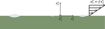
As illustrated in figure 1, the problem is modelled as an advection–diffusion process of a chemically reactive species in three dimensions, with the
 $x_{1}^{\ast }$
–
 $x_{2}^{\ast }$
plane parallel to the heterogeneous surface and the normal direction denoted by
 $x_{3}^{\ast }$
. Here, starred variables denote dimensional quantities. The species concentration
 $C^{\ast }$
is influenced by a bulk shear flow characterized by shear rate
 $\dot{\unicode[STIX]{x1D6FE}}$
and bulk diffusivity of species
 $D$
. The species undergoes a first-order reaction with rate
 $k$
at the reactive domains, and no flux to the inert surface. If the length scale of the problem is
 $a$
, then the diffusion time scale for the problem is
 $a^{2}/D$
. Coupling it with the shear rate (
 $\dot{\unicode[STIX]{x1D6FE}}$
) and the reaction rate (
 $k$
) gives rise to the two dimensionless parameters, the Péclet number (
 $P$
) and the Damköhler number (
 $\unicode[STIX]{x1D705}$
), which capture the effect of flow and reaction dynamics,
 $$\begin{eqnarray}P=\frac{\dot{\unicode[STIX]{x1D6FE}}a^{2}}{D},\quad \unicode[STIX]{x1D705}=\frac{ka}{D}.\end{eqnarray}$$
The dimensionless governing equations (1.2a )–(1.2c ) describe a mixed boundary value problem on an arbitrary heterogeneous surface:
 $$\begin{eqnarray}\displaystyle & \displaystyle \unicode[STIX]{x1D6FB}_{x}^{2}C-Px_{3}\frac{\unicode[STIX]{x2202}C}{\unicode[STIX]{x2202}x_{1}}=0, & \displaystyle\end{eqnarray}$$
 $$\begin{eqnarray}\displaystyle & \displaystyle \frac{\unicode[STIX]{x2202}C}{\unicode[STIX]{x2202}x_{3}}=\unicode[STIX]{x1D705}C\quad \text{on the reactive region},x_{3}=0, & \displaystyle\end{eqnarray}$$
 $$\begin{eqnarray}\displaystyle & \displaystyle \frac{\unicode[STIX]{x2202}C}{\unicode[STIX]{x2202}x_{3}}=0\quad \text{on the inert region},x_{3}=0, & \displaystyle\end{eqnarray}$$
 $\langle C^{\ast }\rangle$
; the reasons for doing so will become evident in § 1.2.1.
Inert disks embedded in a reactive wall in an unbounded surface submerged in a shear flow.

For a reactive region of dimensionless area
 $A$
, the Sherwood number
 $S$
is the area-averaged diffusive mass flux (the convective flux is zero),
 $$\begin{eqnarray}S=\frac{1}{A}\int {\displaystyle \frac{\unicode[STIX]{x2202}C}{\unicode[STIX]{x2202}x_{3}}}\,\text{d}A.\end{eqnarray}$$
Using (1.2b ), the Sherwood number can be expressed as a simple integral of the surface concentration field over the reactive region,
 $$\begin{eqnarray}S=\frac{\unicode[STIX]{x1D705}}{A}\int C\,\text{d}A.\end{eqnarray}$$
In the case of non-zero area fraction (type (
 ${\mathcal{R}}_{p}$
) and (
 ${\mathcal{I}}_{p}$
) surfaces), the above expression is evaluated by simply considering the reactive area in one periodic unit. The Sherwood number is a function of
 $(P,\unicode[STIX]{x1D705},\unicode[STIX]{x1D719})$
and, in general, depends on the configuration of the reactive regions. The above equation will be useful in drawing qualitative conclusions about the Sherwood number in various regimes of parameters once the surface concentration is known.
For surface type (
 ${\mathcal{I}}$
), the length scale,
 $a$
, for the microscale problem is chosen to be the radius of the inert circular disk. For type (
 ${\mathcal{R}}$
) surfaces,
 $a$
is the radius of the reactive disks. Configurations (
 ${\mathcal{R}}_{p}$
) and (
 ${\mathcal{I}}_{p}$
) are referred to as ‘periodic’ while configurations (
 ${\mathcal{R}}_{u}$
) and (
 ${\mathcal{I}}_{u}$
) are called ‘unbounded’ or ‘isolated’. Consistent with the naming of surfaces, we denote all fields and integrals of fields (
 $C_{u},S_{u}$
) in the unbounded case by the subscript
 $u$
. Similarly, all corresponding quantities in the periodic case (
 $C_{p},S_{p}$
) are denoted by the subscript
 $p$
. When a subscript is not present, it should be assumed that a universal statement is being made. The periodicity will be in the Cartesian directions, although the governing equations (§ 2.1) are not restricted by such considerations. Thus, each periodic unit is a rectangular domain composed of both reactive and inert parts.
1.2 Type (
${\mathcal{R}}$
) surfaces

1.2.1 Effective medium properties
As mentioned before, type (
 ${\mathcal{R}}_{u}$
) and (
 ${\mathcal{R}}_{p}$
) surfaces have been analysed in a previous work (Shah & Shaqfeh Reference Shah and Shaqfeh2015), where the concentration field was solved with a boundary integral formulation. Shah & Shaqfeh (Reference Shah and Shaqfeh2015) showed that there is a finite far-field flux that must balance the diffusive flux at the reactive regions on a periodic surface. Analysing this mass balance over a periodic box, the area average of the concentration field at any
 $x_{3}$
plane can be shown to be
 $\langle C_{p}\rangle =1+\unicode[STIX]{x1D719}S_{p}x_{3}$
. This ensures that
 $$\begin{eqnarray}\langle C_{p}\rangle =1\quad \text{at }x_{3}=0,\end{eqnarray}$$
which is consistent with our non-dimensionalization scheme for the concentration field described earlier. The asymptotic boundary condition for a well-posed periodic formulation of (1.2c ) is
 $$\begin{eqnarray}C_{p}\rightarrow 1+\unicode[STIX]{x1D719}S_{p}(\unicode[STIX]{x1D705},P,\unicode[STIX]{x1D719})x_{3}\quad \text{as }x_{3}\rightarrow \infty .\end{eqnarray}$$
The concentration profile was found to asymptotically approach the far-field profile over a distance that scales with the length scale of the reactive domains (
 $a$
). This was called the slip length, which was shown to be smaller than
 $10a$
for a wide range of Péclet numbers. This asymptotic condition also serves to define a mean surface property in the form of the effective Damköhler number
 $$\begin{eqnarray}\unicode[STIX]{x1D705}_{eff}=\unicode[STIX]{x1D719}S_{p}(\unicode[STIX]{x1D705},P,\unicode[STIX]{x1D719}).\end{eqnarray}$$
This condition follows from the matching constraint on the flux from an ‘outer’ length scale
 $H$
(the macroscale) to the ‘inner’ scale
 $a$
(the microscale) (refer to Shah & Shaqfeh Reference Shah and Shaqfeh2015). To illustrate, the mixed boundary condition (1.2b
)–(1.2c
) in the macroscale problem can be replaced by a single reaction condition,
 $D{\unicode[STIX]{x2202}C_{p}}^{\ast }/\unicode[STIX]{x2202}x_{3}^{\ast }=k_{eff}C_{p}^{\ast }$
, where
 $k_{eff}$
is the effective reaction rate. Using a Taylor expansion at
 $x_{3}^{\ast }\ll H$
, we get
 $C^{\ast }=C_{0}^{\ast }+C_{0}^{\ast }x_{3}^{\ast }k_{eff}/D+\cdots \,$
. This matches the inner solution at
 $x_{3}^{\ast }\gg a$
, i.e. the dimensionless form
 $C=C_{0}[1+x_{3}k_{eff}a/D]+\cdots \,$
matches (1.6). This gives us
 $C_{0}=1$
and
 $\unicode[STIX]{x1D719}S_{p}=k_{eff}a/D=\unicode[STIX]{x1D705}_{eff}$
. Traditionally, a simple approximation of the form
 $\unicode[STIX]{x1D705}_{eff}=\unicode[STIX]{x1D719}\unicode[STIX]{x1D705}$
has been used to model a heterogeneous surface with reactive patches. Shah & Shaqfeh (Reference Shah and Shaqfeh2015) demonstrated that this approximation is valid only in the limit of
 $\unicode[STIX]{x1D705}\ll 1$
or
 $\unicode[STIX]{x1D719}\rightarrow 1$
, and (1.7) should be used instead.
1.2.2 The method of resistances and other asymptotic approximations
The most interesting physics in our problem occurs in the extreme limits for each of the parameters (
 $\unicode[STIX]{x1D705},P,\unicode[STIX]{x1D719}$
). Shah & Shaqfeh (Reference Shah and Shaqfeh2015) employed the so-called method of additive resistances (Bartholomew & Farrauto Reference Bartholomew and Farrauto2011), where the Sherwood number is approximated as the inverse of the sum of ‘resistances’,
 $1/\unicode[STIX]{x1D705}$
and
 $1/S_{p}(\infty ,P,\unicode[STIX]{x1D719})$
,
 $$\begin{eqnarray}S_{p}(\unicode[STIX]{x1D705},P,\unicode[STIX]{x1D719})\approx \left(\frac{1}{\unicode[STIX]{x1D705}}+\frac{1}{S_{p}(\infty ,P,\unicode[STIX]{x1D719})}\right)^{-1}.\end{eqnarray}$$
The effect of
 $P$
and
 $\unicode[STIX]{x1D719}$
on the Sherwood number could thus be understood by studying only the diffusion-limited case,
 $\unicode[STIX]{x1D705}=\infty$
. It was numerically observed that in the large-packing-fraction limit of a periodic distribution of reactive disks,
 $$\begin{eqnarray}S_{p}(\infty ,P,\unicode[STIX]{x1D719})\approx \frac{9\unicode[STIX]{x1D719}}{(1-\unicode[STIX]{x1D719})},\quad \unicode[STIX]{x1D719}<0.78.\end{eqnarray}$$
The Sherwood number was obtained by extrapolating between
 $\unicode[STIX]{x1D719}=0$
and the large-packing-fraction limit (1.9a
),
 $$\begin{eqnarray}S_{p}(\infty ,P,\unicode[STIX]{x1D719})\approx \left((S_{u}(\infty ,P))^{3/2}+\left(\frac{9\unicode[STIX]{x1D719}}{1-\unicode[STIX]{x1D719}}\right)^{3/2}\right)^{2/3}.\end{eqnarray}$$
The method of resistances (1.8) then gives the Sherwood number for a given value of (
 $\unicode[STIX]{x1D705},P,\unicode[STIX]{x1D719}$
) up to
 $\unicode[STIX]{x1D719}\approx 0.78$
within 10 % error. However, the asymptotic limit as
 $\unicode[STIX]{x1D719}\rightarrow 1$
remains to be completely understood. It should be noted that in this packing limit, the type (
 ${\mathcal{R}}_{p}$
) surface is equivalent to a reactive surface embedded with periodic inert domains, i.e. a type (
 ${\mathcal{I}}$
) surface. Thus, we choose to study the inverse problem of type (
 ${\mathcal{I}}_{u}$
) and (
 ${\mathcal{I}}_{p}$
) surfaces to examine the regime of
 $\unicode[STIX]{x1D719}>0.78$
and understand the physics when
 $\unicode[STIX]{x1D719}\rightarrow 1$
. The method of resistances is also relevant in deriving approximations for this study.
1.3 Type (
${\mathcal{I}}$
) surfaces

Even though the surfaces we now study are type (
 ${\mathcal{I}}$
), equations (1.6), (1.5) and (1.7) can easily be shown to hold true.
1.3.1 The geometric nature of the problem in the singular limit of
$\unicode[STIX]{x1D719}\rightarrow 1$

The objective of this work is to identify the correct scaling of Sherwood number with vanishing area fraction of the inert disks,
 $(1-\unicode[STIX]{x1D719})$
. From the discussion on the reaction- and diffusion-limited regimes of
 $\unicode[STIX]{x1D705}$
in Shah & Shaqfeh (Reference Shah and Shaqfeh2015), we note that the following conditions must hold true for the Sherwood number and the surface concentration field on the reactive part (refer to (1.4)):
 $$\begin{eqnarray}\displaystyle & \displaystyle C_{p}\approx 0\quad \text{at }\unicode[STIX]{x1D705}\gg 1,\unicode[STIX]{x1D719}<1, & \displaystyle\end{eqnarray}$$
 $$\begin{eqnarray}\displaystyle & \displaystyle C_{p}\approx 1\quad \text{at }\unicode[STIX]{x1D705}\ll 1,\unicode[STIX]{x1D719}<1, & \displaystyle\end{eqnarray}$$
 $$\begin{eqnarray}\displaystyle & \displaystyle S_{p}<\infty \quad \text{at }\unicode[STIX]{x1D705}\gg 1,\unicode[STIX]{x1D719}<1, & \displaystyle\end{eqnarray}$$
 $$\begin{eqnarray}\displaystyle & \displaystyle S_{p}\approx \unicode[STIX]{x1D705}\quad \text{at }\unicode[STIX]{x1D705}\ll 1,\unicode[STIX]{x1D719}<1. & \displaystyle\end{eqnarray}$$
 $C_{u}=\lim _{\unicode[STIX]{x1D719}\rightarrow 1}C_{p}$
, i.e. the limiting case (
 ${\mathcal{I}}_{u}$
) of case (
 ${\mathcal{I}}_{p}$
). Consider the case of Péclet number
 $P=0$
for the sake of this discussion. In the limit as
 $\unicode[STIX]{x1D719}\rightarrow 1$
, the Sherwood number must become equal to the local Damköhler number, i.e.
 $S_{u}=\unicode[STIX]{x1D705}=\lim _{\unicode[STIX]{x1D719}\rightarrow 1}S_{p}$
. Thus, the far-field solution is of the form
 $C\sim 1+\unicode[STIX]{x1D705}x_{3}$
. This is a valid solution if there are no inert defects, in which case the surface concentration field is unity. However, (1.10a
) and (1.10b
) show that the surface concentration on the reactive region in the presence of inert disks must be a function of
 $\unicode[STIX]{x1D705}$
when we take the limit
 $\unicode[STIX]{x1D719}\rightarrow 1$
. Then, taking the limit as
 $\unicode[STIX]{x1D705}\rightarrow \infty$
, we can write
 $$\begin{eqnarray}\lim _{\unicode[STIX]{x1D705}\rightarrow \infty }\lim _{\unicode[STIX]{x1D719}\rightarrow 1}S_{p}=\lim _{\unicode[STIX]{x1D719}\rightarrow 1}\lim _{\unicode[STIX]{x1D705}\rightarrow \infty }S_{p}=\infty .\end{eqnarray}$$
Conditions (1.10c
) and (1.11) show that
 $S_{p}(\unicode[STIX]{x1D705}=\infty ,\unicode[STIX]{x1D719}<1)<\infty$
but
 $\lim _{\unicode[STIX]{x1D719}\rightarrow 1}S_{p}(\unicode[STIX]{x1D705}=\infty ,\unicode[STIX]{x1D719}<1)=\infty$
. Thus,
 $\unicode[STIX]{x1D719}\rightarrow 1$
is a singular limit for the Sherwood number at
 $\unicode[STIX]{x1D705}=\infty$
. Physically, this means that when there is a distribution of inert defects on a purely adsorbing surface, the flux to the surface is limited geometrically by the existence of the defects. The inert defects introduce a finite resistance to mass transfer that must be related to the geometry of the defect. When there are no defects, there is no resistance to mass transfer and the Sherwood number is infinite. Thus, we anticipate that the Sherwood number at
 $\unicode[STIX]{x1D705}=\infty ,P=0$
is
 $O(1/(1-\unicode[STIX]{x1D719})^{m})$
for some exponent
 $m>0$
as
 $\unicode[STIX]{x1D719}\rightarrow 1$
. The problem is geometric in nature since
 $\unicode[STIX]{x1D719}$
is the only parameter in the system when
 $P=0$
and
 $\unicode[STIX]{x1D705}=\infty$
. Shah & Shaqfeh (Reference Shah and Shaqfeh2015) (1.9b
) suggested that
 $m=1$
; however, this correlation was found only over a limited range of
 $\unicode[STIX]{x1D719}$
.
The remainder of this paper is organized as follows. In § 2, we lay the foundations of the boundary element method (BEM) that we use to study our problem numerically. The governing equations and the boundary conditions of our problem are linear and are amenable to the machinery of Green’s functions and boundary integral methods. The computational details are not the same as those in Shah & Shaqfeh (Reference Shah and Shaqfeh2015). The primary difference is that we solve the boundary integral equations in a Galerkin formulation instead of a collocation scheme, allowing easy extrapolation of nodal values for analysis. The boundary integral equation further serves a theoretical purpose in § 3, where we derive the scaling for the Sherwood number in the limit as
 $\unicode[STIX]{x1D719}\rightarrow 1$
using perturbation analysis for small
 $(1-\unicode[STIX]{x1D719})$
. We improve the results of the perturbation analysis by proposing a ‘non-interacting periodic’ approximation, i.e. we use the solution for type (
 ${\mathcal{I}}_{u}$
) surfaces to study type (
 ${\mathcal{I}}_{p}$
) surfaces in § 4. A number of important results are obtained and justified, including demonstration of the existence of a surface concentration boundary layer (when
 $\unicode[STIX]{x1D705}\gg 1$
) surrounding the inert disk and the failure of the method of resistances (when
 $(1-\unicode[STIX]{x1D719})\ll 1$
). Finally, a general approximation for the Sherwood number is derived in § 5 and compared with BEM simulation results. We conclude that our approximation is valid for a wide range of the Damköhler and Péclet numbers, and we end with a discussion on the nature of such a correlation in § 6. We finish with a remark on the geometric nature of the problem in the limit of
 $\unicode[STIX]{x1D719}\rightarrow 1$
and the relationship to the case study of Shah & Shaqfeh (Reference Shah and Shaqfeh2015).
2 Boundary element method
2.1 The fundamental periodic solution
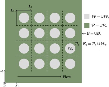
We study the case of transport to a planar reactive surface with periodic planar arrays of inert disks of unit radius. The problem formulation and solution method are exactly the same as those in Shah & Shaqfeh (Reference Shah and Shaqfeh2015). Here, we reproduce brief relevant parts of Shah & Shaqfeh (Reference Shah and Shaqfeh2015) to introduce the notation used throughout this work. The heterogeneous surface
 ${\mathcal{B}}$
is subdivided into identical boxes
 ${\mathcal{B}}_{\boldsymbol{n}}$
(so that
 ${\mathcal{B}}=\cup {\mathcal{B}}_{\boldsymbol{n}}$
), where
 $\boldsymbol{n}\in \mathbb{Z}^{2}$
. Each such unit has the same configuration of reactive and inert domains, denoted by
 ${\mathcal{P}}_{\boldsymbol{n}}$
and
 ${\mathcal{W}}_{\boldsymbol{n}}$
respectively (see figure 2). The entire reactive region is
 ${\mathcal{P}}=\cup {\mathcal{P}}_{\boldsymbol{n}}$
, while the inert region is
 ${\mathcal{W}}=\cup {\mathcal{W}}_{\boldsymbol{n}}$
. The area of the reactive region in each box is denoted by
 $P_{0}=|{\mathcal{P}}_{\boldsymbol{n}}|$
, while that for the inert region is
 $W_{0}=|{\mathcal{W}}_{\boldsymbol{n}}|$
. The centres of each box
 ${\mathcal{B}}_{\boldsymbol{n}}$
form a lattice structure,
 $$\begin{eqnarray}\boldsymbol{r}_{\boldsymbol{n}}=n_{1}\boldsymbol{L}_{1}+n_{2}\boldsymbol{L}_{2}\quad (n_{1},n_{2}=0,\pm 1,\pm 2,\ldots ),\end{eqnarray}$$
where
 $\boldsymbol{L}_{1}$
and
 $\boldsymbol{L}_{2}$
are steps along periodic directions on the heterogeneous surface. All periodic quantities have subscript ‘
 $p$
’. Following (1.2c
) and the asymptotic condition (1.6), the periodic concentration field
 $C_{p}$
satisfies
 $$\begin{eqnarray}\displaystyle & \displaystyle \unicode[STIX]{x1D6FB}_{x}^{2}C_{p}-Px_{3}\frac{\unicode[STIX]{x2202}C_{p}}{\unicode[STIX]{x2202}x_{1}}=0, & \displaystyle\end{eqnarray}$$
 $$\begin{eqnarray}\displaystyle & \displaystyle \frac{\unicode[STIX]{x2202}C_{p}}{\unicode[STIX]{x2202}x_{3}}=\unicode[STIX]{x1D705}C_{p}\quad \text{at }\boldsymbol{x}\in {\mathcal{P}}_{\boldsymbol{n}},\boldsymbol{n}\in \mathbb{Z}^{2}, & \displaystyle\end{eqnarray}$$
 $$\begin{eqnarray}\displaystyle & \displaystyle \frac{\unicode[STIX]{x2202}C_{p}}{\unicode[STIX]{x2202}x_{3}}=0\quad \text{at }\boldsymbol{x}\in {\mathcal{W}}_{\boldsymbol{n}},\boldsymbol{n}\in \mathbb{Z}^{2}, & \displaystyle\end{eqnarray}$$
 $$\begin{eqnarray}\displaystyle & \displaystyle C_{p}\rightarrow 1+\frac{P_{0}}{B_{0}}S_{p}(\unicode[STIX]{x1D705},P,\unicode[STIX]{x1D719})x_{3}\quad \text{as }x_{3}\rightarrow \infty . & \displaystyle\end{eqnarray}$$
A periodic system of reactive region
 ${\mathcal{P}}_{\boldsymbol{n}}$
with inert disks
 ${\mathcal{W}}_{\boldsymbol{n}}$
embedded in corresponding bounding boxes
 ${\mathcal{B}}_{\boldsymbol{n}}$
. Shear flow of strength
 $\dot{\unicode[STIX]{x1D6FE}}$
is present in the wall-normal direction. Also illustrated are the periodicity directions
 $\boldsymbol{L}_{1},\boldsymbol{L}_{2}$
in the lattice.

The Sherwood number,
 $S_{p}$
, is identical for each porous region
 ${\mathcal{P}}_{\boldsymbol{n}}$
, and is given by the expression
 $$\begin{eqnarray}S_{p}(\unicode[STIX]{x1D705},P,\unicode[STIX]{x1D719})=\frac{1}{|{\mathcal{P}}_{\boldsymbol{n}}|}\int _{{\mathcal{P}}_{\boldsymbol{n}}}\unicode[STIX]{x1D705}C_{p}(\boldsymbol{x}_{b})\,\text{d}A(\boldsymbol{x}_{b}),\end{eqnarray}$$
where the subscript ‘
 $b$
’ on the dummy variable indicates that point
 $\boldsymbol{x}_{b}$
is bound to the surface
 ${\mathcal{B}}$
. Shah & Shaqfeh (Reference Shah and Shaqfeh2015) devised a BEM that uses the Green’s function,
 $G_{p}$
, that satisfies the adjoint problem described in (2.4a–c
) below. It should be noted that the subscript ‘
 $s$
’ denotes the
 $_{1},_{2}$
coordinates.
 $$\begin{eqnarray}\displaystyle & \displaystyle \unicode[STIX]{x1D6FB}^{2}G_{p}+Px_{3}\frac{\unicode[STIX]{x2202}G_{p}}{\unicode[STIX]{x2202}x_{1}}=-\unicode[STIX]{x1D6FF}(x_{3}-y_{3})\left(\unicode[STIX]{x1D6FF}^{2}(\boldsymbol{x}_{s}-\boldsymbol{y}_{s,\boldsymbol{n}})-\frac{1}{B_{0}}\right), & \displaystyle\end{eqnarray}$$
 $$\begin{eqnarray}\displaystyle & \displaystyle \frac{\unicode[STIX]{x2202}G_{p}}{\unicode[STIX]{x2202}x_{3}}=0\quad \text{at }\boldsymbol{x}\in {\mathcal{B}}_{\boldsymbol{n}}, & \displaystyle\end{eqnarray}$$
 $$\begin{eqnarray}\displaystyle & \displaystyle G_{p}\rightarrow 0\quad \text{as }x_{3}\rightarrow \infty . & \displaystyle\end{eqnarray}$$
 $\unicode[STIX]{x1D6FF}^{2}(\boldsymbol{x}_{s}-\boldsymbol{y}_{s,\boldsymbol{n}})$
is a Dirac comb (Córdoba Reference Córdoba1989), i.e. a periodic distribution of singularities at
 $\boldsymbol{y}_{\boldsymbol{n}}=(\boldsymbol{y}_{s,\boldsymbol{n}},y_{3})$
, where
 $$\begin{eqnarray}\boldsymbol{y}_{s,\boldsymbol{n}}=\boldsymbol{y}_{s,0}+n_{1}\boldsymbol{L}_{1}+n_{2}\boldsymbol{L}_{2}\quad (n_{1},n_{2}=0,\pm 1,\pm 2,\ldots ).\end{eqnarray}$$
The renormalization term (Hasimoto Reference Hasimoto1959; Sangani & Behl Reference Sangani and Behl1989)
 $1/B_{0}$
balances the flux of singularity per periodic box. When the periodic singularities
 $\boldsymbol{y}_{b}$
(subscript
 $\boldsymbol{n}$
dropped for clarity) are bound to the surface
 ${\mathcal{B}}$
, we have (Shah & Shaqfeh Reference Shah and Shaqfeh2015)
 $$\begin{eqnarray}G_{p}(\boldsymbol{x}|\boldsymbol{y}_{b};P)=\frac{1}{B_{0}}\mathop{\sum }_{k\neq 0}\frac{-\text{Ai}(s)}{\text{Ai}^{\prime }(s_{0})(\text{i}Pk_{1})^{1/3}}\text{e}^{-\text{i}\boldsymbol{k}\boldsymbol{\cdot }(\boldsymbol{x}_{s}-\boldsymbol{y}_{s})},\end{eqnarray}$$
where
 $$\begin{eqnarray}s=\frac{k^{2}+\text{i}Pk_{1}x_{3}}{(\text{i}Pk_{1})^{2/3}}\quad \text{and }\quad s_{0}=\frac{k^{2}}{(\text{i}Pk_{1})^{2/3}},\end{eqnarray}$$
and
 $\boldsymbol{k}=(k_{1},k_{2})$
are vectors in the reciprocal lattice,
 $$\begin{eqnarray}\displaystyle & \displaystyle \boldsymbol{k}=2\unicode[STIX]{x03C0}n_{1}\boldsymbol{l}_{1}+2\unicode[STIX]{x03C0}n_{2}\boldsymbol{l}_{2}\quad (n_{1},n_{2}=0,\pm 1,\pm 2,\ldots ), & \displaystyle\end{eqnarray}$$
 $$\begin{eqnarray}\displaystyle & \displaystyle \text{where}\quad \boldsymbol{l}_{1}=\frac{\boldsymbol{L}_{2}\times \hat{x}_{3}}{B_{0}},\quad \boldsymbol{l}_{2}=\frac{\hat{x}_{3}\times \boldsymbol{L}_{1}}{B_{0}}, & \displaystyle\end{eqnarray}$$
 $$\begin{eqnarray}\displaystyle & \displaystyle \text{so}\quad \boldsymbol{k}\boldsymbol{\cdot }\boldsymbol{L}_{t}=2\unicode[STIX]{x03C0}n_{t}\quad (t=1,2). & \displaystyle\end{eqnarray}$$
Shah & Shaqfeh (Reference Shah and Shaqfeh2015) then derive a boundary integral equation for the periodic concentration field using the periodic Green’s function as the kernel,
 $$\begin{eqnarray}C_{p}(\boldsymbol{x})=1+\unicode[STIX]{x1D719}S_{p}x_{3}-\unicode[STIX]{x1D705}\int _{{\mathcal{P}}_{0}}G_{p}(\boldsymbol{y}_{b}|\boldsymbol{x};P)C_{p}(\boldsymbol{y}_{b})\,\text{d}A(\boldsymbol{y}_{b}).\end{eqnarray}$$
The Sherwood number
 $S_{p}$
is determined self-consistently by the following procedure.
-
(i) Solve (2.9) for
$C_{p}(\boldsymbol{x}_{b})$
on
${\mathcal{P}}_{0}$
. -
(ii) Obtain
$S_{p}(\unicode[STIX]{x1D705},P,\unicode[STIX]{x1D719})$
using (2.3). -
(iii) Generate
$C_{p}(\boldsymbol{x})$
in the bulk as the left-hand side of (2.9).


The boundary integral equations are solved by meshing the reactive region over which the integral is defined and using the Galerkin approach to solve for nodal concentrations in the mesh. As the integral equations are periodic, we effectively solve by meshing the reactive region in only one periodic subunit.
2.2 Numerical implementation of the BEM
The Fourier series in (2.6) is evaluated at a grid point using Evald’s summation technique (Hasimoto Reference Hasimoto1959), as described in Shah & Shaqfeh (Reference Shah and Shaqfeh2015). The Green’s function at any point is then calculated using a bilinear interpolation between the values at the four grid points surrounding it. The integral equation (2.9) is solved numerically by converting to matrix equations using a Galerkin method on triangular elements for the reactive region, and this method differs from that presented in Shah & Shaqfeh (Reference Shah and Shaqfeh2015). Let the set of nodes be indexed by labels from the set
 ${\mathcal{N}}=\{i\}$
. The value of the concentration field at the node
 $i$
is denoted by
 $C_{i}$
, which is to be determined. We use piecewise continuous linear shape functions
 $\unicode[STIX]{x1D713}_{i}(\boldsymbol{x})$
centred at node
 $i$
. We solve the following set of linear equations for
 $C_{i}$
:
 $$\begin{eqnarray}\langle \unicode[STIX]{x1D713}_{j}(\boldsymbol{x}),1\rangle C_{j}+\unicode[STIX]{x1D705}\mathop{\sum }_{i\in {\mathcal{N}}}\langle \unicode[STIX]{x1D713}_{j}(\boldsymbol{x}),\langle G(\boldsymbol{x}_{0}|\boldsymbol{x};P),\unicode[STIX]{x1D713}_{i}(\boldsymbol{x}_{0})\rangle \rangle C_{i}=\langle \unicode[STIX]{x1D713}_{j}(\boldsymbol{x}),1\rangle ,\quad j\in {\mathcal{N}},\end{eqnarray}$$
where the standard
 $L_{2}$
inner product
 $\langle \cdot \,,\cdot \rangle$
is defined for periodic functions
 $f,g$
by an integral over the reactive region
 ${\mathcal{P}}_{0}$
inside one periodic box,
 $$\begin{eqnarray}\langle f(\boldsymbol{x}),g(\boldsymbol{x})\rangle =\int _{{\mathcal{P}}_{0}}f(\boldsymbol{x})g(\boldsymbol{x})\,\text{d}A(\boldsymbol{x}).\end{eqnarray}$$
The Green’s function has an integrable singularity at
 $\boldsymbol{x}=\boldsymbol{x}_{0}$
, and special care must be taken while evaluating the double inner product in (2.10) when
 $i=j$
. The surface concentration field and the Sherwood number are then approximately given by
 $$\begin{eqnarray}\displaystyle & \displaystyle C_{p}(\boldsymbol{x})\approx \mathop{\sum }_{j\in {\mathcal{N}}}C_{j}\unicode[STIX]{x1D713}_{j}(\boldsymbol{x}), & \displaystyle\end{eqnarray}$$
 $$\begin{eqnarray}\displaystyle & \displaystyle S_{p}(\unicode[STIX]{x1D705},P,\unicode[STIX]{x1D719})\approx \frac{\unicode[STIX]{x1D705}}{P_{0}}\mathop{\sum }_{j\in {\mathcal{N}}}\langle \unicode[STIX]{x1D713}_{j}(\boldsymbol{x}),1\rangle C_{j}. & \displaystyle\end{eqnarray}$$
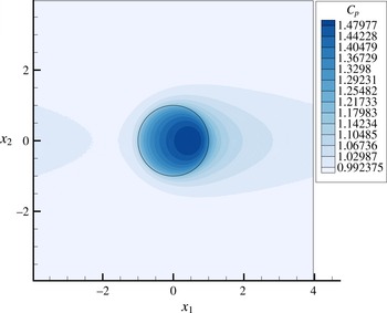
Figure 3 shows the contours of the surface concentration field for a sample simulation with parameters
 $\unicode[STIX]{x1D705}=1,P=20$
and
 $\unicode[STIX]{x1D719}=0.95$
. One can observe that a concentration wake exists downstream of the inert patch. This wake is a concentration accretion region, similar in shape to the depletion region observed around the reactive disk in type (
 ${\mathcal{R}}_{u}$
) surfaces. The far-field surface concentration field is approximately
 $C_{p}\approx 1$
, while the concentration field inside the inert patch is significantly higher than everywhere else.
Contour plot of surface concentration for the case of periodic inert disks embedded in a reactive wall;
 $\unicode[STIX]{x1D705}=1,P=20,\unicode[STIX]{x1D719}=0.95$
.

Before we investigate the results of the BEM simulations, we shall derive a scaling law for the Sherwood number at
 $\unicode[STIX]{x1D719}\rightarrow 1$
. This will provide physical intuition for the findings of the BEM simulations. Importantly, we note that since the radius of the inert disks is fixed to unity, the
 $\unicode[STIX]{x1D719}\rightarrow 1$
limit is approached by taking
 $B_{0}\rightarrow \infty$
.
3 Scaling analysis: perturbation approach
Continuing the discussion at the end of § 1.2.2, we recall that the concentration field on the reactive domains must be a function of
 $\unicode[STIX]{x1D705}$
in the limit as
 $\unicode[STIX]{x1D719}\rightarrow 1$
(1.10a,b
). We denote the area fraction of the inert region as
 $$\begin{eqnarray}\unicode[STIX]{x1D6FF}=1-\unicode[STIX]{x1D719}.\end{eqnarray}$$
Then, in the limit as
 $\unicode[STIX]{x1D6FF}\rightarrow 0$
, we write the surface concentration in the reactive region as
 $$\begin{eqnarray}C_{p}=\frac{\unicode[STIX]{x1D719}S_{p}(\unicode[STIX]{x1D705},P,\unicode[STIX]{x1D719})}{\unicode[STIX]{x1D705}}+C_{p}^{(1)}.\end{eqnarray}$$
Equation (3.2) guarantees that the surface concentration field is a function of
 $\unicode[STIX]{x1D705}$
in general. It also implies that the leading-order value of
 $C_{p}$
is
 $O(1)$
when
 $\unicode[STIX]{x1D6FF}\rightarrow 0$
or
 $\unicode[STIX]{x1D705}\ll 1$
. Thus, the form of (3.2) is consistent with the reaction- and diffusion-limited regimes of the Damköhler number (1.10a–d
). Equation (3.2) can also be viewed as a statement that the local concentration flux
 $\unicode[STIX]{x1D705}C_{p}$
is approximately uniform and matches the asymptotic flux in (1.6). However, the expansion (3.2) is still an assumption that requires justification. Equation (3.2) is valid only when
 $C_{p}^{(1)}$
is small compared with the leading-order term throughout the reactive domain – an assumption to which we shall return later.
Substituting (3.2) in the boundary integral equation (2.9), we obtain, at
 $x_{3}=0$
,
 $$\begin{eqnarray}C_{p}=1-\unicode[STIX]{x1D719}S_{p}\int _{{\mathcal{P}}_{0}}G_{p}(\boldsymbol{y}_{b}|\boldsymbol{x}_{b};P)\,\text{d}A(\boldsymbol{y}_{b})-\unicode[STIX]{x1D705}\int _{{\mathcal{P}}_{0}}G_{p}(\boldsymbol{y}_{b}|\boldsymbol{x}_{b};P)C_{p}^{(1)}(\boldsymbol{y}_{b})\,\text{d}A(\boldsymbol{y}_{b}).\end{eqnarray}$$
We integrate the above equation over the reactive region
 ${\mathcal{P}}_{0}$
. It should be noted that when the integrand is periodic, one can make the following switch:
 $\int _{{\mathcal{P}}_{0}}(\cdot )=-\int _{{\mathcal{W}}_{0}}(\cdot )$
. Finally, we use (1.4) to write
 $$\begin{eqnarray}\displaystyle P_{0}\frac{S_{p}}{\unicode[STIX]{x1D705}}-P_{0} & = & \displaystyle -\unicode[STIX]{x1D719}S_{p}\int _{{\mathcal{W}}_{0}}\int _{{\mathcal{W}}_{0}}G_{p}(\boldsymbol{y}_{b}|\boldsymbol{x}_{b};P)\,\text{d}A(\boldsymbol{y}_{b})\,\text{d}A(\boldsymbol{x}_{b})\nonumber\\ \displaystyle & & \displaystyle +\,\unicode[STIX]{x1D705}\int _{{\mathcal{W}}_{0}}\int _{{\mathcal{P}}_{0}}G_{p}(\boldsymbol{y}_{b}|\boldsymbol{x}_{b};P)C_{p}^{(1)}(\boldsymbol{y}_{b})\,\text{d}A(\boldsymbol{y}_{b})\,\text{d}A(\boldsymbol{x}_{b}).\end{eqnarray}$$
Due to the assumption in (3.2) that
 $C_{p}^{(1)}$
is small everywhere, the first integral on the right-hand side is the dominant term, which balances the left-hand side, and we get
 $$\begin{eqnarray}P_{0}\frac{S_{p}}{\unicode[STIX]{x1D705}}\approx P_{0}-\unicode[STIX]{x1D719}S_{p}\int _{{\mathcal{W}}_{0}}\int _{{\mathcal{W}}_{0}}G_{p}(\boldsymbol{y}_{b}|\boldsymbol{x}_{b};P)\,\text{d}A(\boldsymbol{y}_{b})\,\text{d}A(\boldsymbol{x}_{b}).\end{eqnarray}$$
The double integral involving
 $G_{p}$
is a function of the Péclet number and shape of the inert domains. In the limit as
 $\unicode[STIX]{x1D6FF}\rightarrow 0$
(i.e.
 $B_{0}\rightarrow \infty$
), the Fourier summation in the Green’s function (2.6) is replaced with the appropriate Fourier integral. Let us denote the double integral in the limit as
 $\unicode[STIX]{x1D6FF}\rightarrow 0$
by
 $f(P)$
,
 $$\begin{eqnarray}f(P)=\int _{{\mathcal{W}}_{0}}\int _{{\mathcal{W}}_{0}}G_{u}(\boldsymbol{y}_{b}|\boldsymbol{x}_{b};P)\,\text{d}A(\boldsymbol{y}_{b})\,\text{d}A(\boldsymbol{x}_{b}),\end{eqnarray}$$
where (see Shah & Shaqfeh Reference Shah and Shaqfeh2015)
 $$\begin{eqnarray}G_{u}(\boldsymbol{x}|\boldsymbol{y}_{b};P)=\frac{1}{(2\unicode[STIX]{x03C0})^{2}}\int _{-\infty }^{\infty }\int _{-\infty }^{\infty }\frac{-\text{Ai}(s)}{\text{Ai}^{\prime }(s_{0})(\text{i}Pk_{1})^{1/3}}\text{e}^{-\text{i}\boldsymbol{k}\boldsymbol{\cdot }(\boldsymbol{x}_{s}-\boldsymbol{y}_{s})}\,\text{d}k_{1}\text{d}k_{2}.\end{eqnarray}$$
Here,
 $G_{u}$
is the Green’s function for an isolated singularity and is useful in solving for the concentration field for the isolated reactive disk in type (
 ${\mathcal{R}}_{u}$
) surfaces. Noting that
 $P_{0}=B_{0}\unicode[STIX]{x1D719}=W_{0}\unicode[STIX]{x1D719}/\unicode[STIX]{x1D6FF}$
, a rearrangement of the terms in (3.5) yields
 $$\begin{eqnarray}\frac{1}{S_{p}(\unicode[STIX]{x1D705},P,\unicode[STIX]{x1D719})}\approx \left(\frac{1}{\unicode[STIX]{x1D705}}+\frac{\unicode[STIX]{x1D6FF}f(P)}{W_{0}}\right).\end{eqnarray}$$
This scaling form is reminiscent of the method of resistances approximation (see (1.8)) and implies that the method of resistances is valid even when
 $\unicode[STIX]{x1D719}\rightarrow 1$
. In particular, (3.8a
) suggests that
 $$\begin{eqnarray}\frac{1}{S_{p}(\infty ,P,\unicode[STIX]{x1D719})}\approx \frac{\unicode[STIX]{x1D6FF}f(P)}{W_{0}}.\end{eqnarray}$$
The results (3.8a
) and (3.8b
) have significant implications. First, they appear to validate the scaling used in the approximation (1.9b
). Second, even without having determined the coefficient of scaling,
 $f(P)$
, one can already expect that
 $1/f(P)$
will exhibit a
 $P^{1/3}$
scaling at large Péclet number, corresponding to the Graetz Leveque limit for
 $S_{p}(\infty ,P,\unicode[STIX]{x1D719})$
.
The scaling constant
 $f(P)$
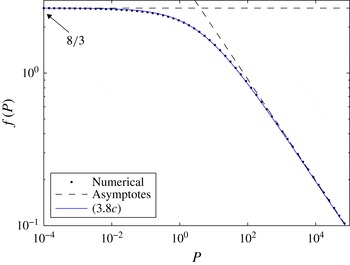
in (3.6) is obtained by numerical integration of the Green’s function in (3.7) and then fitting an approximation that exhibits the correct asymptotes, as detailed in appendix A,
 $$\begin{eqnarray}\frac{f(P)}{W_{0}}\approx \frac{8}{3\unicode[STIX]{x03C0}}\left(1+\left(1.5778P^{-1/3}\right)^{-15/8}\right)^{-8/15}.\end{eqnarray}$$
Here,
 $W_{0}=\unicode[STIX]{x03C0}$
for circular defects. As will become evident from figures 6 and 8, when
 $\unicode[STIX]{x1D705}\gg 1$
, equations (3.8a
)–(3.8c
) deviate from the ‘correct’ values of the Sherwood number predicted numerically using the BEM. This means that the last integral term in (3.4) cannot be ignored in the diffusion-limited regime of the Damköhler number. Thus, we anticipate that
 $C_{p}^{(1)}$
is not always small in the reactive domain on the surface. To overcome this difficulty, we propose a new approach in the following section. To explain this approach, we need the solution
 $C_{u}$
to the problem of a single inert disk in a reactive surface (type (
 ${\mathcal{I}}_{u}$
) surface).
4 Scaling analysis: non-interacting periodic inert disks
Consider the problem statement for type (
 ${\mathcal{I}}_{u}$
) surfaces,
 $$\begin{eqnarray}\displaystyle & \displaystyle \unicode[STIX]{x1D6FB}_{x}^{2}C_{u}-Px_{3}\frac{\unicode[STIX]{x2202}C_{u}}{\unicode[STIX]{x2202}x_{1}}=0, & \displaystyle\end{eqnarray}$$
 $$\begin{eqnarray}\displaystyle & \displaystyle \frac{\unicode[STIX]{x2202}C_{u}}{\unicode[STIX]{x2202}x_{3}}=\unicode[STIX]{x1D705}C_{u}\quad \text{at }\boldsymbol{x}\in {\mathcal{P}}, & \displaystyle\end{eqnarray}$$
 $$\begin{eqnarray}\displaystyle & \displaystyle \frac{\unicode[STIX]{x2202}C_{u}}{\unicode[STIX]{x2202}x_{3}}=0\quad \text{at }\boldsymbol{x}\in {\mathcal{W}}, & \displaystyle\end{eqnarray}$$
 $$\begin{eqnarray}\displaystyle & \displaystyle C_{u}\rightarrow 1+\unicode[STIX]{x1D705}x_{3}\quad \text{as }x_{3}\rightarrow \infty . & \displaystyle\end{eqnarray}$$
When
 $\unicode[STIX]{x1D6FF}\rightarrow 0$
, the surface concentration field
 $C_{p}$
just around the inert disk in type (
 ${\mathcal{I}}_{p}$
) surfaces is not influenced by periodicity, and must match the unbounded case concentration field
 $C_{u}$
, up to a multiplicative constant. From the perturbation expansion (3.2), the far-field surface concentration is uniform to the leading order (
 $C_{p}\approx \unicode[STIX]{x1D719}S_{p}/\unicode[STIX]{x1D705}$
), while the correction
 $C_{p}^{(1)}$
must account for the non-uniform concentration around the inert region, particularly, as we shall see, when
 $\unicode[STIX]{x1D705}\gg 1$
. Thus, one may postulate the following ‘non-interacting periodic’ approximation to first order in
 $\unicode[STIX]{x1D6FF}$
for the surface concentration field:
 $$\begin{eqnarray}C_{p}\approx \frac{\unicode[STIX]{x1D719}S_{p}}{\unicode[STIX]{x1D705}}C_{u}\quad \text{at }\unicode[STIX]{x1D6FF}\ll 1.\end{eqnarray}$$
To rigorously characterize the validity of (4.2), we examine the respective boundary integral equations for type (
 ${\mathcal{I}}_{u}$
) and (
 ${\mathcal{I}}_{p}$
) surfaces. For type (
 ${\mathcal{I}}_{u}$
) surfaces, the integral equation is written using the unbounded Green’s function,
 $$\begin{eqnarray}C_{u}(\boldsymbol{x})=1+\unicode[STIX]{x1D705}x_{3}-\unicode[STIX]{x1D705}\int _{{\mathcal{P}}}G_{u}(\boldsymbol{y}_{b}|\boldsymbol{x};P)(C_{u}(\boldsymbol{y}_{b})-1)\,\text{d}A(\boldsymbol{y}_{b})+\unicode[STIX]{x1D705}\int _{{\mathcal{W}}}G_{u}(\boldsymbol{y}_{b}|\boldsymbol{x};P)\,\text{d}A(\boldsymbol{y}_{b}).\end{eqnarray}$$
Let
 $C^{E}=C_{p}-(\unicode[STIX]{x1D719}S_{p}/\unicode[STIX]{x1D705})C_{u}$
denote the error in (4.2). Multiplying (4.3) by
 $\unicode[STIX]{x1D719}S_{p}/\unicode[STIX]{x1D705}$
and subtracting from (2.9), and leaving out higher-order terms on the right-hand side, gives the following integral equation for the error (see appendix C for derivation details) when
 $\unicode[STIX]{x1D6FF}\ll 1$
:
 $$\begin{eqnarray}C^{E}=\left(1-\frac{\unicode[STIX]{x1D719}S_{p}}{\unicode[STIX]{x1D705}}\right)-\unicode[STIX]{x1D705}\int _{{\mathcal{P}}_{0}}G_{u}C^{E}\,\text{d}A-\unicode[STIX]{x1D719}S_{p}\int _{{\mathcal{W}}_{0}}(G_{u}-G_{p})\,\text{d}A.\end{eqnarray}$$
The difference between the periodic and unbounded Green’s functions is
 $O(\unicode[STIX]{x1D6FF}^{1/2})$
, as shown in Shah & Shaqfeh (Reference Shah and Shaqfeh2015). It should be recalled that
 $S_{p}=\unicode[STIX]{x1D705}+o(\unicode[STIX]{x1D705})$
when
 $\unicode[STIX]{x1D705}\ll 1$
. On the other hand, when
 $\unicode[STIX]{x1D705}\gg 1$
, we expect that
 $S_{p}=O(\unicode[STIX]{x1D6FF}^{-1})$
, as foreshadowed by (3.8b
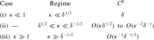
). Thus, we are interested in the balance of terms in (4.4) when (i)
 $\unicode[STIX]{x1D705}\ll \unicode[STIX]{x1D6FF}^{1/2}$
, (ii)
 $\unicode[STIX]{x1D6FF}^{1/2}\ll \unicode[STIX]{x1D705}\ll \unicode[STIX]{x1D6FF}^{-1/2}$
and (iii)
 $\unicode[STIX]{x1D6FF}^{-1/2}\ll \unicode[STIX]{x1D705}$
. Case (i) corresponds to when
 $\unicode[STIX]{x1D705}\ll 1$
. Here,
 $\unicode[STIX]{x1D6FF},\unicode[STIX]{x1D705}$
are the small parameters, as we assume that
 $C^{E}=O(\unicode[STIX]{x1D705}^{n}\unicode[STIX]{x1D6FF}^{m}),m\geqslant 0,n\geqslant 0$
. Thus, we can write the following balance between the left-hand side and the right-hand side when
 $\unicode[STIX]{x1D705}\ll 1$
:
 $O(\unicode[STIX]{x1D705}^{n}\unicode[STIX]{x1D6FF}^{m})=\unicode[STIX]{x1D6FF}+O(\unicode[STIX]{x1D705}^{n+1}\unicode[STIX]{x1D6FF}^{m})+O(\unicode[STIX]{x1D705}\unicode[STIX]{x1D6FF}^{1/2})$
. Then, for case (i), the left-hand side balances the dominant order on the right-hand side,
 $\unicode[STIX]{x1D6FF}$
, yielding
 $m=1,n=0$
. The error is
 $C^{E}=\unicode[STIX]{x1D6FF}$
to the leading order.
Summary of the error scalings in the non-interacting approximation (4.2) for various regimes of
 $\unicode[STIX]{x1D705}$
with respect to
 $\unicode[STIX]{x1D6FF}$
.

Case (iii) corresponds to the case when
 $\unicode[STIX]{x1D705}\gg 1$
. Now,
 $\unicode[STIX]{x1D6FF},\unicode[STIX]{x1D705}^{-1}$
are the small parameters, and the balance between the terms on the left-hand side and the right-hand side is represented as
 $O(\unicode[STIX]{x1D705}^{-n}\unicode[STIX]{x1D6FF}^{m})=O(1)+O(\unicode[STIX]{x1D705}^{-1}\unicode[STIX]{x1D6FF}^{-1})+O(\unicode[STIX]{x1D705}^{1-n}\unicode[STIX]{x1D6FF}^{m})+O(\unicode[STIX]{x1D6FF}^{-1/2})$
. The last term on the right-hand side dominates the
 $O(1)$
term, and the left-hand side is strictly dominated by the third term on the right-hand side. Multiplying by
 $\unicode[STIX]{x1D705}^{-1}$
throughout, the exponents
 $m,n$
must be determined by the balance between the terms
 $O([\unicode[STIX]{x1D705}\unicode[STIX]{x1D6FF}^{1/2}]^{-2}),O(\unicode[STIX]{x1D705}^{-n}\unicode[STIX]{x1D6FF}^{m})$
and
 $O([\unicode[STIX]{x1D705}\unicode[STIX]{x1D6FF}^{1/2}]^{-1})$
, corresponding to the last three on the right-hand side. We immediately observe that for case (iii), we have
 $m=-1/2,n=1$
and the error is
 $C^{E}=O(\unicode[STIX]{x1D705}^{-1}\unicode[STIX]{x1D6FF}^{-1/2})$
.
The conditions for case (ii) can still hold when
 $\unicode[STIX]{x1D705}\ll 1$
or
 $\unicode[STIX]{x1D705}\gg 1$
. Performing an analysis for each subcase, one can show that the error scale changes from
 $O(\unicode[STIX]{x1D705}\unicode[STIX]{x1D6FF}^{1/2})$
when
 $\unicode[STIX]{x1D705}\ll 1$
to
 $O(\unicode[STIX]{x1D705}^{-2}\unicode[STIX]{x1D6FF}^{-1})$
when
 $\unicode[STIX]{x1D705}\gg 1$
. The errors in these three cases are presented in table 1. To summarize, the non-interacting approximation has small error at small values of the Damköhler number when
 $\unicode[STIX]{x1D6FF}$
is sufficiently small. The error is small also at large values of the Damköhler number (
 $\unicode[STIX]{x1D705}\unicode[STIX]{x1D6FF}^{1/2}\gg 1$
). We will revisit this in our discussion of the boundary layer structure in § 4.2. Once we calculate
 $C_{u}$
, we can assess the accuracy of the non-interacting approximation by comparing the surface concentration profiles corresponding to (4.2) and those calculated from the BEM simulations. As mentioned before, we use (4.2) to develop new correlations for the Sherwood number. The accuracy and regimes of validity of (4.2) will also be evident from the comparison between the Sherwood number from the BEM simulations and the new correlations in § 5.
4.1 Concentration field
$C_{u}$
for a single inert patch in a reactive surface

At
 $P=0$
, the concentration field
 $C_{u}$
satisfies the axisymmetric Laplace equation and the solution may be expressed naturally in cylindrical coordinates (
 $\unicode[STIX]{x1D70C}=(x_{1}^{2}+x_{2}^{2})^{1/2},x_{3}$
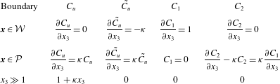
). The solution is calculated as a superposition of three fields, each satisfying the Laplace equation but with different boundary and far-field asymptotic conditions that are summarized in table 2,
 $$\begin{eqnarray}\displaystyle C_{u} & = & \displaystyle \tilde{C_{u}}+(1+\unicode[STIX]{x1D705}x_{3}),\end{eqnarray}$$
 $$\begin{eqnarray}\displaystyle \tilde{C_{u}} & = & \displaystyle -\unicode[STIX]{x1D705}C_{1}+C_{2}.\end{eqnarray}$$
The term
 $C_{1}$
has a well-known closed-form solution (Gladwell, Barber & Olesiak Reference Gladwell, Barber and Olesiak1983) which can be expressed in Legendre polynomials and functions of spheroidal coordinates (
 $\unicode[STIX]{x1D70C}=\cosh \unicode[STIX]{x1D709}\sin \unicode[STIX]{x1D702},x_{3}=\sinh \unicode[STIX]{x1D709}\cos \unicode[STIX]{x1D6FD}$
),
 $$\begin{eqnarray}C_{1}=\frac{2}{\unicode[STIX]{x03C0}}Q_{1}(\text{i}\sinh \unicode[STIX]{x1D709})P_{1}(\cos \unicode[STIX]{x1D702}).\end{eqnarray}$$
On the heterogeneous surface, this simplifies to
 $$\begin{eqnarray}\displaystyle & \displaystyle C_{1}=\left\{\begin{array}{@{}ll@{}}-\displaystyle \frac{2}{\unicode[STIX]{x03C0}}(1-\unicode[STIX]{x1D70C}^{2})^{1/2}\quad & \text{at }x_{3}=0,\unicode[STIX]{x1D70C}<1,\\ 0\quad & \text{at }x_{3}=0,\unicode[STIX]{x1D70C}\geqslant 1,\end{array}\right. & \displaystyle\end{eqnarray}$$
 $$\begin{eqnarray}\displaystyle & \displaystyle {\displaystyle \frac{\unicode[STIX]{x2202}C_{1}}{\unicode[STIX]{x2202}x_{3}}}=\left\{\begin{array}{@{}ll@{}}0\quad & \quad \text{at }x_{3}=0,\unicode[STIX]{x1D70C}<1,\\ \displaystyle R(\unicode[STIX]{x1D70C})=\frac{2}{\unicode[STIX]{x03C0}}\left(\arcsin \left(\frac{1}{\unicode[STIX]{x1D70C}}\right)-\frac{1}{\unicode[STIX]{x1D70C}}\left(1-\frac{1}{\unicode[STIX]{x1D70C}^{2}}\right)^{-1/2}\right)\quad & \quad \text{at }x_{3}=0,\unicode[STIX]{x1D70C}\geqslant 1.\end{array}\right. & \displaystyle\end{eqnarray}$$
The above forms of
 $C_{1}$
and its normal gradient
 $\unicode[STIX]{x2202}C_{1}/\unicode[STIX]{x2202}x_{3}$
will be useful in developing correlations and understanding the structure of the concentration field (when
 $\unicode[STIX]{x1D705}\gg 1$
) in the ensuing sections. The solution form for
 $C_{2}$
involves a tedious spectral expansion and is not presented here. The solution technique to obtain both
 $C_{1}$
and
 $C_{2}$
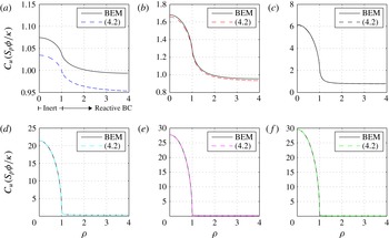
is outlined in detail in Gladwell et al. (Reference Gladwell, Barber and Olesiak1983). The total concentration profile as a function of the radial position from the centre of the inert disk is shown in figure 4 for the case of
 $\unicode[STIX]{x1D6FF}=0.05$
. One can see that the far-field surface concentration quickly approaches a constant value
 $C_{p}\approx \unicode[STIX]{x1D719}S_{p}/\unicode[STIX]{x1D705}$
for
 $\unicode[STIX]{x1D705}>1$
. The field inside the inert disk is seen to grow large at large
 $\unicode[STIX]{x1D705}$
while the far-field solution decays to zero. This is consistent with the fact that the average surface concentration is unity. The concentration profile as predicted by (4.2) matches the profile calculated using BEM simulations, especially at
 $\unicode[STIX]{x1D705}\gg 1$
. At
 $\unicode[STIX]{x1D705}=0.1$
, the relative error in the concentration profile is approximately
 $0.05$
, which is in fact
 $O(\unicode[STIX]{x1D6FF})$
. This validates the non-interacting periodic approximation (4.2) over a wide range of values of the Damköhler number, and confirms our error analysis of table 1. It is important to note that the Sherwood number
 $S_{p}$
used in figure 4 is the one obtained from the converged BEM simulations.
Summary of boundary conditions for various field variables.

The surface concentration profiles as calculated using the ‘non-interacting periodic’ approximation (4.2) (dashed) and solving the BEM equations (2.9) (thin, black) are plotted for various values of
 $\unicode[STIX]{x1D705}$
and
 $\unicode[STIX]{x1D719}=0.95$
, i.e.
 $\unicode[STIX]{x1D6FF}=0.05$
, and
 $P=0.001$
. The Sherwood number in the multiplying constant
 $\unicode[STIX]{x1D719}S_{p}/\unicode[STIX]{x1D705}$
of equation (4.2) is calculated using the BEM simulations. Indeed, the non-interacting periodic approximation works very well as the Damköhler number becomes large.
 $\unicode[STIX]{x1D705}=0.1$
(a), 1 (b), 10 (c), 100 (d), 300 (e), 500 (f).

4.2 Boundary layer in the surface concentration field around the inert patch
As claimed before, (3.8a
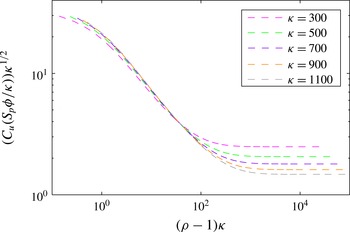
) is not universally correct as there exists (see figure 4) a surface concentration boundary layer surrounding the inert disk, due to which the last integral in (3.4) can no longer be assumed to be small. We plot the surface concentration field,
 $C_{p}=\unicode[STIX]{x1D719}S_{p}C_{u}/\unicode[STIX]{x1D705}$
, as a function of the distance from the inert disk boundary,
 $\unicode[STIX]{x1D70C}-1$
, in figure 5 for large values of the Damköhler number. Again, it should be noted that here
 $S_{p}$
is obtained from BEM simulations. When
 $C_{p}$
is scaled by
 $\unicode[STIX]{x1D705}^{1/2}$
and the distance from the disk boundary is scaled by
 $\unicode[STIX]{x1D705}$
, all of the curves collapse to a single curve close to the disk boundary, as seen in figure 5. This proves that the boundary layer thickness scales with
 $1/\unicode[STIX]{x1D705}$
while the surface concentration field scales with
 $\unicode[STIX]{x1D705}^{-1/2}$
. Since the normal gradient is related to the surface concentration via (2.2b
), the local flux just outside the inert disk scales with
 $\unicode[STIX]{x1D705}^{1/2}$
. This deserves an in-depth discussion, for which we re-examine (4.5) and (4.6) along with the individual boundary conditions in table 2.
It should be noted that since
 $C_{1}=0$
on the reactive region (from (4.8)), the surface concentration field is given by
 $C_{u}=1+C_{2}$
. Thus, when
 $\unicode[STIX]{x1D705}\ll 1$
, we see that the surface concentration field is, as expected,
 $C_{u}\approx 1$
. When
 $\unicode[STIX]{x1D705}\gg 1$
, it should be noted that
 $C_{2}$
approximately satisfies the boundary condition
 $-C_{2}=\unicode[STIX]{x2202}C_{1}/\unicode[STIX]{x2202}x_{3}$
with an error of
 $O(1/\unicode[STIX]{x1D705})$
. Using the known solution (4.9), we obtain the following asymptotic expansion near the edge of the inert disk:
 $C_{u}\approx (2/\unicode[STIX]{x03C0})(\unicode[STIX]{x1D70C}-1)^{-1/2}$
at
 $\unicode[STIX]{x1D70C}\rightarrow 1^{+}$
. Consequently, from the non-interacting approximation, it follows that
 $C_{p}\sim (1/\unicode[STIX]{x1D705})(\unicode[STIX]{x1D70C}-1)^{-1/2}$
, where we used (1.10c
) to substitute
 $\unicode[STIX]{x1D719}S_{p}/\unicode[STIX]{x1D705}\sim 1/\unicode[STIX]{x1D705}$
. Equivalently, from the reaction condition (2.2b
), the local surface flux at
 $\unicode[STIX]{x1D705}\gg 1$
is given by
 $\unicode[STIX]{x2202}C_{p}/\unicode[STIX]{x2202}x_{3}\sim (\unicode[STIX]{x1D70C}-1)^{-1/2}$
. This form is reminiscent of the well-known singularity (Stone Reference Stone1989) in the surface flux at the disk boundary for an isothermal disk in an insulating surface, which is the type (
 ${\mathcal{R}}$
) counterpart to this problem. It follows immediately from the asymptotic forms of
 $C_{p}$
and
 $\unicode[STIX]{x2202}C_{p}/\unicode[STIX]{x2202}x_{3}$
that if the boundary layer thickness
 $\unicode[STIX]{x1D70C}-1$
scales with
 $1/\unicode[STIX]{x1D705}$
, the surface concentration field
 $C_{p}$
near the disk edge must scale with
 $\unicode[STIX]{x1D705}^{-1/2}$
. Indeed, the collapsed curves in figure 5 display a slope of
 $-1/2$
, corresponding to the
 $1/(\unicode[STIX]{x1D70C}-1)^{1/2}$
decay.
The boundary layer structure provides insight as to when the non-interacting approximation (4.2) breaks down. As the boundary layer thickness scales with
 $1/\unicode[STIX]{x1D705}$
, when
 $\unicode[STIX]{x1D705}\ll \unicode[STIX]{x1D6FF}^{1/2}$
, the boundary layer must scale with a length larger than the size of the periodic box. In such a case, the ‘inner’ surface concentration scales on the size of the periodic box and is not screened from the periodic influence of the domain. Thus, (4.2) then leads to errors of size
 $\unicode[STIX]{x1D6FF}$
, as noted before in figure 4(a).
A rescaled surface concentration field is plotted versus the distance from the disk boundary for
 $P=0.001$
. Boundary layer existence and scaling is apparent from the fact that all of the curves approach a constant curve in the limit as
 $\unicode[STIX]{x1D705}\rightarrow \infty$
.

5 Approximations for
$S_{p}$
in the dilute limit of inert defects

In this section, we present correlations for
 $S_{p}$
using the non-interacting approximation. In § 5.1, we consider
 $P=0$
to understand the coupling of reaction with geometry. In 5.2, we consider
 $P>0$
to understand the effect of flow.
5.1 Case I: no flow,
$P=0$

The non-interacting periodic inert disk approximation leads to an alternative more accurate approximation for the Sherwood number in type (
 ${\mathcal{I}}_{p}$
) surfaces (periodic inert disks). The key idea is to recognize that
 $\int _{{\mathcal{W}}_{0}}C_{p}(\boldsymbol{x}_{b})\,\text{d}A(\boldsymbol{x}_{b})+\int _{{\mathcal{P}}_{0}}C_{p}(\boldsymbol{x}_{b})\,\text{d}A(\boldsymbol{x}_{b})=B_{0}$
, which is a consequence of the average surface concentration being unity (see (1.5)). The integral over the reactive surface
 ${\mathcal{P}}$
is simply
 $P_{0}S_{p}/\unicode[STIX]{x1D705}$
(see (1.4)). Using the non-interacting periodic approximation and the relations
 $P_{0}=W_{0}\unicode[STIX]{x1D719}/\unicode[STIX]{x1D6FF},B_{0}=W_{0}/\unicode[STIX]{x1D6FF}$
, we can write
 $(\unicode[STIX]{x1D719}S_{p}/\unicode[STIX]{x1D705}W_{0})\int _{{\mathcal{W}}_{0}}C_{u}(\boldsymbol{x}_{b})\,\text{d}A(\boldsymbol{x}_{b})=1/\unicode[STIX]{x1D6FF}-\unicode[STIX]{x1D719}/\unicode[STIX]{x1D6FF}(S_{p}/\unicode[STIX]{x1D705})$
. This simplifies to
 $$\begin{eqnarray}S_{p}(\unicode[STIX]{x1D705},P=0,\unicode[STIX]{x1D719})=\frac{\unicode[STIX]{x1D705}}{\unicode[STIX]{x1D719}+\unicode[STIX]{x1D719}\unicode[STIX]{x1D6FF}\displaystyle \left[\frac{1}{W_{0}}\int _{{\mathcal{W}}_{0}}C_{u}(\boldsymbol{x}_{b})\,\text{d}A(\boldsymbol{x}_{b})\right]}.\end{eqnarray}$$
The surface integral above can be written as a sum of surface integrals of
 $C_{1}$
and
 $C_{2}$
(4.5)–(4.6). The surface integral of
 $C_{2}$
can be represented as a summation involving the spectral coefficients (Gladwell et al.
Reference Gladwell, Barber and Olesiak1983), while
 $C_{1}$
can be explicitly integrated using the closed-form expression (4.8). The final form of the surface integral of
 $C_{u}$
in (5.1) is given by
 $$\begin{eqnarray}\frac{1}{W_{0}}\int _{{\mathcal{W}}_{0}}C_{u}(\boldsymbol{x}_{b})\,\text{d}A(\boldsymbol{x}_{b})=1+\frac{4\unicode[STIX]{x1D705}}{3\unicode[STIX]{x03C0}}+\text{corr}(\unicode[STIX]{x1D705}),\end{eqnarray}$$
where the integral involving
 $C_{2}$
contributes a ‘correction’ term
 $\text{corr}(\unicode[STIX]{x1D705})$
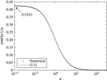
. We fit the following Padé approximant (figure 14, appendix B) using least squares with less than 1 % error:
 $$\begin{eqnarray}\frac{\text{corr}(\unicode[STIX]{x1D705})}{\unicode[STIX]{x1D705}}=\frac{4}{3\unicode[STIX]{x03C0}}\left(\frac{0.8837}{\unicode[STIX]{x1D705}^{0.6809}+0.8837}\right).\end{eqnarray}$$
The prefactor
 $4/3\unicode[STIX]{x03C0}$
has been taken out to emphasize that
 $\text{corr}(\unicode[STIX]{x1D705})/\unicode[STIX]{x1D705}\approx 4/3\unicode[STIX]{x03C0}$
at
 $\unicode[STIX]{x1D705}\ll 1$
. Using equations (5.1), (5.2) and (5.3), one can write the following improved approximation for the Sherwood number:
 $$\begin{eqnarray}\displaystyle S_{p}(\unicode[STIX]{x1D705},P=0,\unicode[STIX]{x1D719}) & = & \displaystyle \frac{\unicode[STIX]{x1D705}}{\unicode[STIX]{x1D719}+\unicode[STIX]{x1D719}\unicode[STIX]{x1D6FF}\unicode[STIX]{x1D705}\displaystyle \left[\frac{1}{\unicode[STIX]{x1D705}}+\frac{4}{3\unicode[STIX]{x03C0}}+\frac{\text{corr}(\unicode[STIX]{x1D705})}{\unicode[STIX]{x1D705}}\right]},\end{eqnarray}$$
 $$\begin{eqnarray}\displaystyle & = & \displaystyle \frac{\unicode[STIX]{x1D705}}{\unicode[STIX]{x1D719}+\unicode[STIX]{x1D719}\unicode[STIX]{x1D6FF}\unicode[STIX]{x1D705}\displaystyle \left[\frac{1}{\unicode[STIX]{x1D705}}+\frac{4}{3\unicode[STIX]{x03C0}}\left(1+\frac{0.8837}{\unicode[STIX]{x1D705}^{0.6809}+0.8837}\right)\right]}.\end{eqnarray}$$
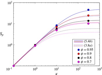
The Sherwood number
 $S_{p}(\unicode[STIX]{x1D705},0,\unicode[STIX]{x1D719})$
is plotted as a function of the Damköhler number at various values of the area fraction
 $\unicode[STIX]{x1D719}$
. The approximation (5.4b
) (thin lines) matches very well the ‘exact’ values of the Sherwood number obtained from BEM simulations (filled circles). The perturbation approximation (3.8a
) (dotted) is valid only when
 $\unicode[STIX]{x1D705}\ll 1$
.

The Sherwood number as predicted by (5.4b
) is plotted as a function of the Damköhler number in figure 6 for various values of
 $\unicode[STIX]{x1D719}$
. Certainly, the approximation (5.4b
) is very good in predicting the ‘exact’ Sherwood number obtained from BEM simulations. As expected, the approximation is better as we approach
 $\unicode[STIX]{x1D719}\rightarrow 1$
.
The inverse of the Sherwood number is plotted at large
 $\unicode[STIX]{x1D705}$
(
 $\unicode[STIX]{x1D705}=300$
) to demonstrate the scaling with
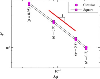
 $\unicode[STIX]{x1D6FF}\unicode[STIX]{x1D719}$
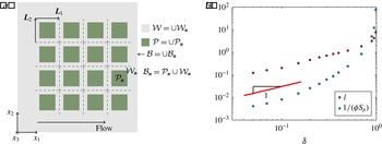
as observed in (5.5). For both inert disks (filled circles) and squares (filled boxes), the same scaling is observed.

The form of (5.4b
) warrants a discussion. In particular, at
 $\unicode[STIX]{x1D705}=\infty$
, the term corresponding to the correction in the denominator is zero and we are left with an expression that is purely a function of the area fraction of disks,
 $$\begin{eqnarray}S_{p}(\unicode[STIX]{x1D705}=\infty ,P=0,\unicode[STIX]{x1D719})=\frac{3\unicode[STIX]{x03C0}}{4\unicode[STIX]{x1D6FF}\unicode[STIX]{x1D719}}.\end{eqnarray}$$
Thus, equation (5.5) confirms the purely geometric nature of the problem in the diffusion-limited regime of type (
 ${\mathcal{I}}_{p}$
) surfaces. The prefactor
 $3\unicode[STIX]{x03C0}/4$
is a ‘shape factor’ corresponding to the disk-shaped inert patches. Indeed, for the case of square inert patches, we find evidence for a different prefactor in figure 7. Here, results for both disk- and square-shaped patches are shown at
 $\unicode[STIX]{x1D705}\gg 1$
. Intriguingly, this prefactor appears to be weakly shape-dependent. Sadhal & Tio (Reference Sadhal and Tio1991) showed that the contact resistance for the case of heat transfer between conducting solids with periodic circular adiabatic gaps (corresponding directly to the case of
 $P=0,\unicode[STIX]{x1D705}=\infty$
) grows as
 $1/\unicode[STIX]{x1D6FF}$
to the leading order at
 $\unicode[STIX]{x1D6FF}\ll 1$
, which is a confirmation of (5.5).
The term
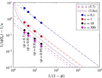
 $1/(\unicode[STIX]{x1D719}S_{p})-1/\unicode[STIX]{x1D705}$
scales linearly with
 $1/(1-\unicode[STIX]{x1D719})$
at all values of the Damköhler number, as suggested by (5.7) and proved by the Sherwood number obtained from BEM simulations. The perturbation approximation (3.8a
) (dotted) is valid only when
 $\unicode[STIX]{x1D705}\ll 1$
. The Péclet number is set to zero here.

To demonstrate the importance of the boundary layer at
 $\unicode[STIX]{x1D705}\gg 1$
, observe that for the corresponding perturbation series approximation (3.8b
), the shape factor for the disk is
 $3\unicode[STIX]{x03C0}/8$
, which is half of the correct shape factor. Knowing the boundary layer structure from § 4.2, when
 $\unicode[STIX]{x1D705}\gg 1$
, we can write
 $C_{p}\approx (\unicode[STIX]{x1D719}S_{p}/\unicode[STIX]{x1D705})C_{u}\approx (\unicode[STIX]{x1D719}S_{p}/\unicode[STIX]{x1D705})(1-\unicode[STIX]{x2202}C_{1}/\unicode[STIX]{x2202}x_{3})$
. Matching this with the perturbation expansion (3.2), we get
 $C_{p}^{(1)}=-(\unicode[STIX]{x1D719}S_{p}/\unicode[STIX]{x1D705})(\unicode[STIX]{x2202}C_{1}/\unicode[STIX]{x2202}x_{3})$
. Using this relation for
 $C_{p}^{(1)}$
along with (4.9) and the unbounded Green’s function for
 $P=0$
, we can now analytically calculate the term neglected in the perturbation approximation in (3.4) (details are given in appendix D),
 $$\begin{eqnarray}\displaystyle & & \displaystyle \unicode[STIX]{x1D705}\int _{{\mathcal{W}}_{0}}\int _{{\mathcal{P}}_{0}}G_{p}(\boldsymbol{y}_{b}|\boldsymbol{x}_{b};0)C_{p}^{(1)}(\boldsymbol{y}_{b})\,\text{d}A(\boldsymbol{y}_{b})\,\text{d}A(\boldsymbol{x}_{b})\nonumber\\ \displaystyle & & \displaystyle \quad =\unicode[STIX]{x1D719}S_{p}\int _{{\mathcal{W}}_{0}}\int _{{\mathcal{P}}_{0}}\frac{-1}{2\unicode[STIX]{x03C0}\Vert \boldsymbol{x}_{b}-\boldsymbol{y}_{b}\Vert }{\displaystyle \frac{\unicode[STIX]{x2202}C_{1}(\boldsymbol{y}_{b})}{\unicode[STIX]{x2202}y_{3}}}\,\text{d}A(\boldsymbol{y}_{b})\,\text{d}A(\boldsymbol{x}_{b})\nonumber\\ \displaystyle & & \displaystyle \quad =\frac{4}{3}\unicode[STIX]{x1D719}S_{p}.\end{eqnarray}$$
An immediate consequence of (5.6) is that (3.4) now reads as
 $P_{0}S_{p}/\unicode[STIX]{x1D705}=P_{0}-\unicode[STIX]{x1D719}S_{p}f(0)+4\unicode[STIX]{x1D719}S_{p}/3$
at
 $P=0$
. As
 $f(0)=8/3$
(see (3.8c
)), the corrected version of (3.8b
) for circular disks is given by
 $1/S_{p}(\infty ,0,\unicode[STIX]{x1D719})=(4/3)\unicode[STIX]{x1D6FF}/\unicode[STIX]{x03C0}$
, which now has the correct shape factor. Thus, neglect of the last term in (3.4) leads to drastically different predicted values of the Sherwood number in figure 6 at
 $\unicode[STIX]{x1D705}\gg 1$
. For a different geometry of the inert patches, one can expect the Sherwood number
 $S_{p}(\unicode[STIX]{x1D705}=\infty ,P=0,\unicode[STIX]{x1D719})$
to scale with
 $1/(\unicode[STIX]{x1D6FF}\unicode[STIX]{x1D719})$
with a different shape factor due to the geometric nature of the limit
 $\unicode[STIX]{x1D705}\rightarrow \infty$
.
The Sherwood number
 $S_{p}(\unicode[STIX]{x1D705},P,\unicode[STIX]{x1D719})$
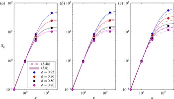
is plotted as a function of the Damköhler number at various values of the area fraction
 $\unicode[STIX]{x1D719}$
for the cases (a)
 $P=0.001$
, (b)
 $P=2$
and (c)
 $P=20$
. The approximation (5.8) (thin lines) matches very well the ‘exact’ values of the Sherwood number obtained from BEM simulations (filled circles). The
 $P=0$
approximation (dashed lines, (5.4b
)) is inaccurate at
 $P=20$
.

Casting (5.4b ) as
 $$\begin{eqnarray}\frac{1}{\unicode[STIX]{x1D719}S_{p}(\unicode[STIX]{x1D705},0,\unicode[STIX]{x1D719})}=\frac{1}{\unicode[STIX]{x1D705}}+(1-\unicode[STIX]{x1D719})\left[\frac{1}{\unicode[STIX]{x1D705}}+\frac{4}{3\unicode[STIX]{x03C0}}\left(1+\frac{0.8837}{\unicode[STIX]{x1D705}^{0.6809}+0.8837}\right)\right],\end{eqnarray}$$
we see that any approximation based on the method of resistances (for example, (3.8a
)) fails as it is very different from (5.7). First, there is an additional multiplying factor
 $\unicode[STIX]{x1D719}$
for the Sherwood number on the left-hand side of (5.7). Second, the last term on the right-hand side now depends on the Damköhler number. The scaling of this last term is evident from the plot of
 $1/(\unicode[STIX]{x1D719}S_{p})-1/\unicode[STIX]{x1D705}$
versus
 $1/(1-\unicode[STIX]{x1D719})$
at various values of the Damköhler number in figure 8. Specifically, we see that the Sherwood number in (5.7), which is based on the non-interacting approximation (4.2), closely matches the values predicted by the BEM simulations at
 $\unicode[STIX]{x1D705}\gg 1$
and
 $\unicode[STIX]{x1D6FF}\ll 1$
. At small Damköhler number and
 $\unicode[STIX]{x1D6FF}>0.1$
, (5.7) deviates from the BEM data because of the errors of size
 $O(\unicode[STIX]{x1D6FF})$
or
 $O(\unicode[STIX]{x1D6FF}^{1/2}\unicode[STIX]{x1D705})$
in the non-interacting approximation (4.2) (see table 1). For the range of
 $\unicode[STIX]{x1D6FF}$
shown in figure 8, the maximum error in (5.7) occurs at
 $\unicode[STIX]{x1D705}=O(1)$
. Nonetheless, the relative error in the Sherwood number in (5.4b
) seen from the data in figure 6 is less than 2 %.
5.2 Case II: shear flow,
$P>0$

To summarize, we first obtained a perturbation series based approximation for the Sherwood number, which resembles the method of resistances form in § 3. We then showed the existence of a surface concentration boundary layer (at
 $\unicode[STIX]{x1D705}\gg 1$
) using the non-interacting periodic disk approach in § 4, which led to an improved correlation (5.4b
) that is valid only when
 $P=0$
. We observe that when the Damköhler number is small (
 $\unicode[STIX]{x1D705}<1$
), the correction term is
 $\text{corr}(\unicode[STIX]{x1D705})/\unicode[STIX]{x1D705}\approx 4/(3\unicode[STIX]{x03C0})$
. Thus, in this regime of the Damköhler number and at vanishingly small area fraction of disks, (5.7) is similar in form to (3.8a
) with
 $f(0)/W_{0}=8/(3\unicode[STIX]{x03C0})$
(see (3.8c
)). Taking inspiration from this, to capture the effect of flow in our correlations, we bridge the approximation (3.8c
) for
 $f(P)$
in (3.8a
) with the last term in (5.7) and hypothesize the following universal approximation:
 $$\begin{eqnarray}S_{p}(\unicode[STIX]{x1D705},P,\unicode[STIX]{x1D719})=\frac{\unicode[STIX]{x1D705}}{\unicode[STIX]{x1D719}+\displaystyle \unicode[STIX]{x1D719}\unicode[STIX]{x1D6FF}\unicode[STIX]{x1D705}\left[\frac{1}{\unicode[STIX]{x1D705}}+\left(\left(\frac{4}{3\unicode[STIX]{x03C0}}+\frac{\text{corr}(\unicode[STIX]{x1D705})}{\unicode[STIX]{x1D705}}\right)^{-15/8}+\left(\frac{4.2075}{\unicode[STIX]{x03C0}}P^{-1/3}\right)^{-15/8}\right)^{-8/15}\right]},\end{eqnarray}$$
where
 $\text{corr}(\unicode[STIX]{x1D705})/\unicode[STIX]{x1D705}$
is given by (5.3). At
 $P=0$
, we recover (5.4b
), while the above correlation also matches the perturbation approximation when
 $\unicode[STIX]{x1D705}\ll 1$
by virtue of its construction. To understand the validity of this approximation, we plot the equivalent of figures 6 and 8 for the Péclet numbers
 $P=0.001,2$
and
 $20$
in figures 9 and 10 respectively. We again observe that the predictions of the new correlation are close to the values of the Sherwood number obtained from BEM simulations. The various correlations valid for the case of
 $\unicode[STIX]{x1D6FF}\ll 1$
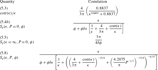
are summarized in table 3. Other than having the correct behaviour in limiting cases, we also have a mathematical explanation for why (5.8) is a good match to BEM results for such a wide range of Péclet numbers. Noting that our error analysis of the non-interacting approximation (4.2) is valid for any Péclet number, we hypothesize that the area-averaging procedure leading to equation (5.1) must hold true and any errors observed must be introduced in the evaluation of the integral term
 $\int _{{\mathcal{P}}_{0}}C_{p}(\boldsymbol{x}_{b})\,\text{d}A(\boldsymbol{x}_{b})$
. These errors stem from leaving out the accretion wake that extends from the inert disk to the outside due to shear flow. These errors will be small as long as the accretion wake does not spread over a large area compared with the reactive region
 ${\mathcal{P}}_{0}$
.
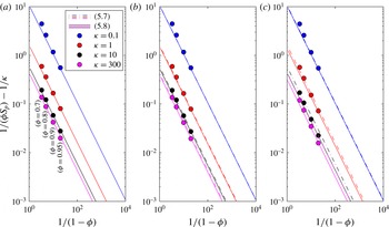
The term
 $1/(\unicode[STIX]{x1D719}S_{p})-1/\unicode[STIX]{x1D705}$
scales linearly with
 $1/(1-\unicode[STIX]{x1D719})$
at all values of the Damköhler number over a wide range of the Péclet number (
 $P\in \{0.001,2,20\}$
) (a–c), as suggested by (5.7) and (5.8) and proved by the Sherwood number obtained from BEM simulations.

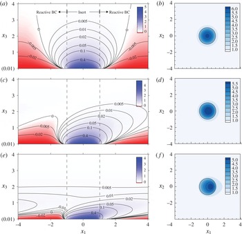
This is indeed confirmed by the contour plots in figure 11 for Péclet numbers ranging from
 $0.001$
to
 $20$
and the corresponding data points in figure 9. Referring to figure 11(a,c,e), as the Péclet number increases, the accretion wake shifts downstream and becomes flatter, and its thickness scales with the boundary layer thickness. This is further shown by figure 11(b,d,f), where the wake stretches downstream of the inert patch with increasing Péclet number. This stretching and flattening of the wake region leads to increased Sherwood number. Even at
 $P=20$
, the wake size is comparable to the size of the inert region. Thus, the correlation (5.8) can be expected to be valid at large Péclet numbers as long as the inert disks are sufficiently dilute such that the wakes are not strongly interacting. Equation (5.8) also captures the fact that as the Péclet number is increased, the boundary layer thickness becomes the length scale for transport at the surface and the effect of shear must dominate the effect of reaction. However, at small Damköhler numbers, i.e. in the reaction-limited regime, the
 $1/\unicode[STIX]{x1D705}$
term in the denominator of (5.8) dominates and, as seen in figure 9, the Sherwood number is weakly dependent on the Péclet number. Thus, the rich interaction between the surface inert irregularities, reaction and flow is surprisingly well captured by (5.8).
Contour plots of the concentration field
 $C_{p}-(1+\unicode[STIX]{x1D719}S_{p}x_{3})$
(a,c,e) in the vertical plane (
 $x_{1}$
–
 $x_{3}$
) and
 $C_{p}$
(b,d,f) on the surface (
 $x_{1}$
–
 $x_{2}$
) for a Damköhler number of
 $\unicode[STIX]{x1D705}=10$
and
 $\unicode[STIX]{x1D719}=0.95$
. Here, the boundary layer and wake structure are exposed. Panels (a,b) correspond to
 $P=0.001$
, (c,d) to
 $P=2$
, and (e,f) to
 $P=20$
.

It should be noted that for inert regions of different shapes, one would develop similar correlations in the spirit of (5.8). For instance, we expect the same asymptotic scaling of
 $f(P)/W_{0}$
with
 $P$
at
 $P\gg 1$
, and that of
 $S_{p}$
with
 $\unicode[STIX]{x1D6FF}$
at
 $\unicode[STIX]{x1D705}\gg 1$
. However, we expect that the constants in (3.8c
) and (5.3) will be shape-dependent. In our analysis, the inert patches are always aligned in the shear direction. While the Péclet number is small, the wakes between inert patches do not affect each other and the non-interacting approximation holds. This forms the central argument for the validity of (5.8). Thus, wake sharing (at
 $P\gg 1$
) will be direction-dependent and thus influence the Sherwood number except in the limit
 $\unicode[STIX]{x1D6FF}\ll 1$
. This is supported by the previous study of Shah & Shaqfeh (Reference Shah and Shaqfeh2015), where the Sherwood number for disordered media was found to have the same scaling when
 $\unicode[STIX]{x1D719},\unicode[STIX]{x1D6FF}\sim O(0.1)$
.


6 Concluding remarks and relation to type (
${\mathcal{R}}$
) surfaces

We have derived a general approximation for the Sherwood number (5.8), which is shown numerically to be accurate for a wide range of values of the Damköhler and Péclet numbers for the case of
 $0.7\leqslant \unicode[STIX]{x1D719}<1$
. The explicit analytical form of (5.8) can be readily used to understand the asymptotic scaling of the Sherwood number with respect to the extremes of the Damköhler number, the Péclet number and the reactive area fraction. In comparison, previously we developed the approximation (1.9b
) for the case when
 $\unicode[STIX]{x1D719}<0.78$
, with a comparatively large error of 10 % (Shah & Shaqfeh Reference Shah and Shaqfeh2015). However, it is important to note that the analyses for the periodic type (
 ${\mathcal{R}}_{p}$
) and (
 ${\mathcal{I}}_{p}$
) surfaces are based on apparently different length scales. For the type (
 ${\mathcal{R}}$
) surfaces, we defined the Sherwood number using the radius of the reactive disks as the length scale. The length scale used in the problem for the type (
 ${\mathcal{I}}$
) surfaces is the radius of the inert disks. The general formula to obtain the Sherwood number with the Damköhler number
 $\unicode[STIX]{x1D705}$
and the Péclet number
 $P$
based on a new length scale
 $a^{\prime }=ar$
, from the Sherwood number for the same surface with a length scale
 $a$
, is given by
 $$\begin{eqnarray}S_{p}(\unicode[STIX]{x1D705},P,\unicode[STIX]{x1D719})_{a^{\prime }}=rS_{p}(\unicode[STIX]{x1D705}/r,P/r^{2},\unicode[STIX]{x1D719})_{a}.\end{eqnarray}$$
Thus, the Sherwood number is not a material property as the Damköhler number is not scale-invariant. Hence, one must convert the Sherwood number for one surface type to another to make a meaningful comparison. It follows that the origin of the scaling (1.9a
) for the
 ${\mathcal{R}}_{p}$
surface of reactive disks must imply that the scaling of the inert regions near close packing of the reactive disks in Shah & Shaqfeh (Reference Shah and Shaqfeh2015) is the same as the scaling length for the reactive regions. Indeed, we note that when
 $\unicode[STIX]{x1D719}=0.78$
for reactive disks, we basically have disconnected inert regions trapped between touching closely packed reactive disks, and the scale of the inert regions remains the scale of the radius of the reactive regions, i.e.
 $a$
. Hence, we anticipate that
 $$\begin{eqnarray}S_{p}\sim 1/\unicode[STIX]{x1D6FF}\end{eqnarray}$$
in the limit as
 $\unicode[STIX]{x1D705}\rightarrow \infty$
, as given in (5.5). This explains the result (1.9a
) in Shah & Shaqfeh (Reference Shah and Shaqfeh2015). Moreover, from the boundary layer analysis presented in this paper, we find that the constant of proportionality in this asymptotic relationship will depend explicitly on the accretion boundary layer(s) near the inert regions, which of course will depend on the topology of the inert defects.
(a) Schematic of reactive squares distributed periodically. (b) The slip length
 $l$
and inverse (
 $\unicode[STIX]{x1D719}S_{p}$
) plotted versus
 $\unicode[STIX]{x1D6FF}$
for the case of periodic square reactive domains on an inert surface (type (
 ${\mathcal{R}}_{p}$
) surface). In these calculations,
 $\unicode[STIX]{x1D705}=300,P=0$
. It should be noted that the slip length was calculated by arbitrarily choosing the normal distance at which the maximum relative difference of the microscale concentration from the asymptotic concentration field over the entire periodic domain was 2 %.

For other surface topologies, however (where the relationship between the reactive and inert defect scales is not so simple), we must carefully consider the consequences of (6.1). The Sherwood number must scale as the inverse of the length scale for the normal gradient over the portions of the reactive surface as shown in (1.3). When
 $\unicode[STIX]{x1D705}\rightarrow \infty$
and
 $P=0$
, the only relevant length scale present must be geometric in nature and controlled by the resistance to mass transfer due to the inert regions. We observe that the concentration field approaches the macroscale field
 $C_{p}=1+\unicode[STIX]{x1D719}S_{p}x_{3}$
over a wall-normal distance that scales with the limit
 $\unicode[STIX]{x1D719}\rightarrow 1$
(i.e.
 $\unicode[STIX]{x1D6FF}\rightarrow 0$
). The slip length
 $l$
is the only normal length scale that defines the boundary between the ‘inner’ (microscale) and ‘outer’ (macroscale) problems. It follows then that if one scales the Sherwood number with a geometric scale
 $a$
, the scaling of
 $S_{p}$
in the limit
 $\unicode[STIX]{x1D719}\rightarrow 1$
must be such that
 $$\begin{eqnarray}S_{p}\sim a/l.\end{eqnarray}$$
Moreover, if the scale
 $a$
remains fixed as
 $\unicode[STIX]{x1D719}\rightarrow 1$
, then this result directly gives the scaling for
 $S_{p}$
as that of the inverse slip length.
To check this hypothesis, we performed the following calculations, where we obtained the Sherwood number
 $S_{p}$
and the slip length
 $l$
for a type (
 ${\mathcal{R}}_{u}$
) surface composed of periodic reactive squares (see figure 12
a) of side 2 (in the case of circular disks, the diameter is 2). We examined the scaling of the Sherwood number and the slip length as
 $\unicode[STIX]{x1D719}\rightarrow 1$
by decreasing the size of the periodic box so that the inert regions ultimately had zero ‘thickness’. This topology is different from that considered in the our analysis of isolated defects, as the defects are continuous for all area fractions. Moreover, in this calculation, we have chosen to define the geometric scale as that of the reactive region for all area fractions, but, in the limit of
 $\unicode[STIX]{x1D719}\rightarrow 1$
, this scale is also the fixed scale of the inert regions. The box size ranges from
 $20\times 20$
to
 $2.052\times 2.052$
, corresponding to a reactive area fraction from
 $0.01$
to
 $0.95$
. We did this for a very large Damköhler number and no-flow conditions, for which we anticipate that all resistance to mass transfer is geometric in nature and dominated by the inert regions. From figure 12(b), we see that for
 $\unicode[STIX]{x1D6FF}<0.1$
,
 $S_{p}$
scales with
 $1/\unicode[STIX]{x1D6FF}$
and the slip length is proportional to
 $\unicode[STIX]{x1D6FF}$
. This confirms our hypothesis that the Sherwood number scales with the inverse dimensionless slip length. Moreover, figure 12(b) suggests that even when the inert regions form a ‘continuous phase’ like in figure 12(a), we still observe the scaling
 $S_{p}\sim 1/\unicode[STIX]{x1D6FF}$
when the Sherwood number is defined on a fixed scale and
 $\unicode[STIX]{x1D6FF}\ll 1$
. It should be noted that the slip length and, thus, the location of an effective boundary condition are large when
 $\unicode[STIX]{x1D719}\ll 1$
(see figure 12
b), as it is meaningless to use an effective boundary condition as a substitute in simulations for an almost inert surface with nearly no mass transfer per unit area of the surface.
There may be many applications where complex topologies of reactive/inert regions may be considered and thus many ways in which one might be interested in the limit
 $\unicode[STIX]{x1D719}\rightarrow 1$
(e.g. those in which there is no fixed surface scale). In such cases, (6.1) should be used in making the comparisons among surface topologies. Thus, the Sherwood number may depend in a complex manner on the configuration of the reactive and inert domains for general surfaces.
It must be noted that the self-consistent mathematical formulation, numerical methods and rigorous analysis in the present study can be extended beyond the problem of mass transport into the domain of momentum transport problems, which is of interest to the wider fluid mechanics community. This opens a powerful way to study how slip is introduced in fluid velocity, e.g. by the presence of rough irregularities on a smooth surface, or patterned hydrophobic surfaces. We plan to consider these problems in future work.
Acknowledgements
P.N.S. is supported by the Stanford Graduate Engineering Fellowship and is grateful for the NSF-MRI2 award 0960306 for computational resources used in this work. T.Y.L. is supported by the Department of Defense (DoD) through the National Defense Science and Engineering Graduate Fellowship (NDSEG) Program.
Appendix A. Determining
$f(P)$

The Fourier mode coefficients in (3.7) have an integrable long-distance decay of the form (
 $1/k$
) in the wavevector space. One can subtract it out and integrate it analytically. The residual difference is integrated over a bounded box domain with a size chosen for convergence of the integral. We will use the following identity to simplify some of the integrals we encounter:
 $$\begin{eqnarray}\int _{{\mathcal{W}}_{0}}\text{e}^{-\text{i}\boldsymbol{k}\boldsymbol{\cdot }\boldsymbol{x}_{s}}\,\text{d}A(\boldsymbol{x}_{s})=\frac{2\unicode[STIX]{x03C0}\text{J}_{1}(k)}{k}.\end{eqnarray}$$
Specifically,
 $$\begin{eqnarray}\displaystyle f(P) & = & \displaystyle \int _{{\mathcal{W}}_{0}}\int _{{\mathcal{W}}_{0}}\frac{1}{(2\unicode[STIX]{x03C0})^{2}}\int _{-\infty }^{\infty }\int _{-\infty }^{\infty }\frac{-\text{Ai}(s)}{\text{Ai}^{\prime }(s_{0})(\text{i}Pk_{1})^{1/3}}\text{e}^{-\text{i}\boldsymbol{k}\boldsymbol{\cdot }(\boldsymbol{x}_{s}-\boldsymbol{y}_{s})}\,\text{d}A(\boldsymbol{k})\,\text{d}A(\boldsymbol{y}_{b})\,\text{d}A(\boldsymbol{x}_{b}),\nonumber\\ \displaystyle & & \displaystyle\end{eqnarray}$$
 $$\begin{eqnarray}\displaystyle & = & \displaystyle \int _{-\infty }^{\infty }\int _{-\infty }^{\infty }\frac{-\text{Ai}(s)}{\text{Ai}^{\prime }(s_{0})(\text{i}Pk_{1})^{1/3}}\frac{\text{J}_{1}^{2}(k)}{k^{2}}\,\text{d}A(\boldsymbol{k}).\end{eqnarray}$$
The large-
 $k$
asymptotes of the Fourier coefficients are also simply the Fourier coefficients for the case when
 $P=0$
. They contribute the following to the above integral:
 $$\begin{eqnarray}\displaystyle f(0) & = & \displaystyle \int _{-\infty }^{\infty }\int _{-\infty }^{\infty }\frac{1}{k}\frac{\text{J}_{1}^{2}(k)}{k^{2}}\,\text{d}k_{1}\text{d}k_{2},\nonumber\\ \displaystyle & = & \displaystyle 2\unicode[STIX]{x03C0}\int _{0}^{\infty }\frac{\text{J}_{1}^{2}(k)}{k^{2}}\,\text{d}k,\nonumber\\ \displaystyle & = & \displaystyle 8/3.\end{eqnarray}$$
The residual contribution that depends on the Péclet number is given by
 $$\begin{eqnarray}\displaystyle f_{1}(P)=\int _{-\infty }^{\infty }\int _{-\infty }^{\infty }\left(\frac{-\text{Ai}(s)}{\text{Ai}^{\prime }(s_{0})(\text{i}Pk_{1})^{1/3}}-\frac{1}{k}\right)\frac{\text{J}_{1}^{2}(k)}{k^{2}}\,\text{d}A(\boldsymbol{k}), & & \displaystyle\end{eqnarray}$$
which is integrated numerically. A higher-resolution integral is carried out around the singularity at
 $\boldsymbol{k}=\pmb{{\it 0}}$
. The asymptotic behaviours of
 $f(P)$
with respect to large and small values of the Péclet number can be observed from figure 13. We construct an approximation using the schemes of Churchill & Usagi (Reference Churchill and Usagi1972) to obtain the approximation (3.8c
), which is seen to accurately match the numerical values, as shown in figure 13.
Numerical evaluation of
 $f(P)$
shows that when
 $P\gg 1$
,
 $f(P)\sim P^{-1/3}$
.

Appendix B. Evaluation of
$\text{corr}(\unicode[STIX]{x1D705})$
in (5.3)

The spectral coefficients in the expansion for
 $C_{2}$
(Gladwell et al.
Reference Gladwell, Barber and Olesiak1983) can be used to numerically compute the correction term
 $\text{corr}(\unicode[STIX]{x1D705})=\int _{{\mathcal{W}}_{0}}C_{2}(\boldsymbol{x})\,\text{d}A(\boldsymbol{x})$
. Figure 14 shows the plot of
 $\text{corr}(\unicode[STIX]{x1D705})/\unicode[STIX]{x1D705}$
versus
 $\unicode[STIX]{x1D705}$
. We see that at small values of the Damköhler number, the correction
 $\text{corr}(\unicode[STIX]{x1D705})$
grows approximately linearly with
 $\unicode[STIX]{x1D705}$
, with a rate of
 $4/(3\unicode[STIX]{x03C0})$
. At
 $\unicode[STIX]{x1D705}\gg 1$
, we see that the correction approaches zero asymptotically. This supports the existence of an apparent limit curve observed in figure 5 as the Damköhler number grows large. We use a Padé approximation (5.3) to obtain the least-squares empirical fit (red line). The fitting error is within 1 % of the numerical values, as seen in figure 14.
Numerical evaluation of
 $\text{corr}(\unicode[STIX]{x1D705})$
shows that when
 $\unicode[STIX]{x1D705}\gg 1$
,
 $\text{corr}(\unicode[STIX]{x1D705})/\unicode[STIX]{x1D705}\rightarrow 0$
.

Appendix C. Boundary integral equation for
$C^{E}$

Let the disk
 ${\mathcal{W}}$
for the unbounded concentration coincide with
 ${\mathcal{W}}_{0}$
for the periodic concentration. Denote
 $\unicode[STIX]{x0394}G_{u-p}=G_{u}-G_{p}$
. Subtraction of the boundary integral equation for
 $\unicode[STIX]{x1D719}S_{p}C_{u}/\unicode[STIX]{x1D705}$
(4.3) from (2.9) gives
 $$\begin{eqnarray}\displaystyle \hspace{-20.00003pt}C^{E} & = & \displaystyle \left(1-\frac{\unicode[STIX]{x1D719}S_{p}}{\unicode[STIX]{x1D705}}\right)-\unicode[STIX]{x1D705}\!\int _{{\mathcal{P}}_{0}}\!G_{p}C_{p}\,\text{d}A+\unicode[STIX]{x1D705}\!\int _{{\mathcal{P}}}\frac{\unicode[STIX]{x1D719}S_{p}}{\unicode[STIX]{x1D705}}G_{u}(C_{u}-1)\,\text{d}A-\unicode[STIX]{x1D719}S_{p}\!\int _{{\mathcal{W}}_{0}}\!G_{u}\,\text{d}A,\end{eqnarray}$$
 $$\begin{eqnarray}\displaystyle \hspace{-20.00003pt} & = & \displaystyle \left(1-\frac{\unicode[STIX]{x1D719}S_{p}}{\unicode[STIX]{x1D705}}\right)-\unicode[STIX]{x1D705}\int _{{\mathcal{P}}_{0}}G_{u}C_{p}\,\text{d}A+\unicode[STIX]{x1D705}\int _{{\mathcal{P}}_{0}}\unicode[STIX]{x0394}G_{u-p}C_{p}\,\text{d}A\nonumber\\ \displaystyle \hspace{-20.00003pt} & & \displaystyle +\,\unicode[STIX]{x1D705}\int _{{\mathcal{P}}}\frac{\unicode[STIX]{x1D719}S_{p}}{\unicode[STIX]{x1D705}}G_{u}(C_{u}-1)\,\text{d}A-\unicode[STIX]{x1D719}S_{p}\int _{{\mathcal{W}}_{0}}G_{u}\,\text{d}A,\end{eqnarray}$$
 $$\begin{eqnarray}\displaystyle \hspace{-20.00003pt} & {\approx} & \displaystyle \left(1-\frac{\unicode[STIX]{x1D719}S_{p}}{\unicode[STIX]{x1D705}}\right)-\unicode[STIX]{x1D705}\int _{{\mathcal{P}}_{0}}G_{u}C_{p}\,\text{d}A+\unicode[STIX]{x1D719}S_{p}\int _{{\mathcal{P}}_{0}}\unicode[STIX]{x0394}G_{u-p}C_{u}\,\text{d}A\nonumber\\ \displaystyle \hspace{-20.00003pt} & & \displaystyle +\,\unicode[STIX]{x1D705}\int _{{\mathcal{P}}_{0}}\frac{\unicode[STIX]{x1D719}S_{p}}{\unicode[STIX]{x1D705}}G_{u}(C_{u}-1)\,\text{d}A-\unicode[STIX]{x1D719}S_{p}\int _{{\mathcal{W}}_{0}}G_{u}\,\text{d}A,\end{eqnarray}$$
 $$\begin{eqnarray}\displaystyle \hspace{-20.00003pt} & {\approx} & \displaystyle \left(1-\frac{\unicode[STIX]{x1D719}S_{p}}{\unicode[STIX]{x1D705}}\right)-\unicode[STIX]{x1D705}\int _{{\mathcal{P}}_{0}}G_{u}C^{E}\,\text{d}A+\unicode[STIX]{x1D719}S_{p}\int _{{\mathcal{P}}_{0}}\unicode[STIX]{x0394}G_{u-p}\,\text{d}A\nonumber\\ \displaystyle \hspace{-20.00003pt} & & \displaystyle -\,\unicode[STIX]{x1D719}S_{p}\int _{{\mathcal{P}}_{0}}G_{u}\,\text{d}A-\unicode[STIX]{x1D719}S_{p}\int _{{\mathcal{W}}_{0}}G_{u}\,\text{d}A,\end{eqnarray}$$
 $$\begin{eqnarray}\displaystyle \hspace{-20.00003pt} & = & \displaystyle \left(1-\frac{\unicode[STIX]{x1D719}S_{p}}{\unicode[STIX]{x1D705}}\right)-\unicode[STIX]{x1D705}\int _{{\mathcal{P}}_{0}}G_{u}C^{E}\,\text{d}A-\unicode[STIX]{x1D719}S_{p}\int _{{\mathcal{W}}_{0}}G_{u}\,\text{d}A-\unicode[STIX]{x1D719}S_{p}\int _{{\mathcal{P}}_{0}}G_{p}\,\text{d}A,\end{eqnarray}$$
 $$\begin{eqnarray}\displaystyle \hspace{-20.00003pt} & = & \displaystyle \left(1-\frac{\unicode[STIX]{x1D719}S_{p}}{\unicode[STIX]{x1D705}}\right)-\unicode[STIX]{x1D705}\int _{{\mathcal{P}}_{0}}G_{u}C^{E}\,\text{d}A-\unicode[STIX]{x1D719}S_{p}\int _{{\mathcal{W}}_{0}}(G_{u}-G_{p})\,\text{d}A.\end{eqnarray}$$
Appendix D. Calculation of the last integral term in (3.4)
From (5.6) and (4.9), the neglected term,
 $N$
, is calculated as follows:
 $$\begin{eqnarray}N=-\unicode[STIX]{x1D719}S_{p}\int _{{\mathcal{W}}_{0}}\int _{{\mathcal{P}}_{0}}\frac{1}{\unicode[STIX]{x03C0}^{2}\Vert \boldsymbol{x}_{b}-\boldsymbol{y}_{b}\Vert }\left(\sin ^{-1}\left(\frac{1}{\Vert \boldsymbol{y}_{b}\Vert }\right)-\frac{1}{(\Vert \boldsymbol{y}_{b}\Vert ^{2}-1)^{1/2}}\right)\,\text{d}A(\boldsymbol{y}_{b})\,\text{d}A(\boldsymbol{x}_{b}).\end{eqnarray}$$
Using the multipole expansion for
 $1/\Vert \boldsymbol{x}_{b}-\boldsymbol{y}_{b}\Vert$
(since
 $\Vert \boldsymbol{x}_{b}\Vert <\Vert \boldsymbol{y}_{b}\Vert$
), and denoting
 $\unicode[STIX]{x1D70C}=\Vert \boldsymbol{y}_{b}\Vert$
, we can simplify the integral for the circular disk with respect to
 $\boldsymbol{x}_{b}$
and obtain in the limit of
 $\unicode[STIX]{x1D719}\rightarrow 1$
 $$\begin{eqnarray}N=-\unicode[STIX]{x1D719}S_{p}\frac{1}{\unicode[STIX]{x03C0}^{2}}\int _{{\mathcal{P}}}\left\{\int _{{\mathcal{W}}_{0}}\mathop{\sum }_{l=0}^{\infty }\frac{\Vert \boldsymbol{x}_{b}\Vert ^{l}P_{l}(\cos \unicode[STIX]{x1D703})}{\unicode[STIX]{x1D70C}^{l+1}}\,\text{d}A(\boldsymbol{x}_{b})\right\}\!\left(\sin ^{-1}\!\left(\frac{1}{\unicode[STIX]{x1D70C}}\right)-\frac{1}{(\unicode[STIX]{x1D70C}^{2}-1)^{1/2}}\right)\text{d}A(\boldsymbol{y}_{b}).\end{eqnarray}$$
The odd terms in
 $l$
vanish, yielding
 $$\begin{eqnarray}N=-\frac{2}{\unicode[STIX]{x03C0}}\unicode[STIX]{x1D719}S_{p}\int _{1}^{\infty }\mathop{\sum }_{m=0}^{\infty }\frac{1}{m+1}\left(\frac{\unicode[STIX]{x1D6E4}(m+1/2)}{m!}\right)^{2}\frac{1}{\unicode[STIX]{x1D70C}^{2m+1}}\left(\sin ^{-1}\left(\frac{1}{\unicode[STIX]{x1D70C}}\right)-\frac{1}{(\unicode[STIX]{x1D70C}^{2}-1)^{1/2}}\right)\unicode[STIX]{x1D70C}\,\text{d}\unicode[STIX]{x1D70C}.\end{eqnarray}$$
The definite integral with respect to
 $\unicode[STIX]{x1D70C}$
has an analytical closed form, which leads to an infinite series expression for
 $N$
,
 $$\begin{eqnarray}N=-\frac{2}{\unicode[STIX]{x03C0}}\unicode[STIX]{x1D719}S_{p}\mathop{\sum }_{m=0}^{\infty }\frac{1}{m+1}\left(\frac{\unicode[STIX]{x1D6E4}(m+1/2)}{m!}\right)^{2}\left(\frac{\unicode[STIX]{x03C0}}{2(2m-1)}-\frac{\sqrt{\unicode[STIX]{x03C0}}\unicode[STIX]{x1D6E4}(m+1)}{(2m-1)\unicode[STIX]{x1D6E4}(m+1/2)}\right).\end{eqnarray}$$
Numerically evaluating the above series to within machine error, we get
 $$\begin{eqnarray}N=\frac{4}{3}\unicode[STIX]{x1D719}S_{p}.\end{eqnarray}$$