1 Introduction
Study of the microscopic properties of gas particles and their mutual interactions can be used to generate a statistical framework that describes the macroscopic characteristics of a dilute gas, such as its density, mean velocity and temperature. Utilising particle conservation arguments, this kinetic approach yields the Boltzmann equation, which describes changes in the probabilistic mass distribution function of the gas that result from interparticle collisions and phase space advection. In contrast to the conventional Navier–Stokes–Fourier equation and no-slip condition, which utilise the continuum hypothesis, this approach is valid at arbitrary degrees of gas rarefaction. Such flows are often characterised by the Knudsen number:
 $$\begin{eqnarray}\mathit{Kn}\equiv \frac{{\it\lambda}}{d},\end{eqnarray}$$
where the gas mean free path is
 ${\it\lambda}$
and
 $d$
is a (general) characteristic length scale of the bulk flow. The continuum hypothesis is formally valid in the asymptotic limit of zero Knudsen number (Hadjiconstantinou Reference Hadjiconstantinou2006). However, gas flows generated by modern nanoscale devices, which are tens and hundreds of nanometres in size and exhibit unsteady (oscillatory) motion in a broad frequency range (Bargatin, Kozinsky & Roukes Reference Bargatin, Kozinsky and Roukes2007; Pelton et al.
Reference Pelton, Sader, Burgin, Liu, Guyot-Sionnest and Gosztola2009; Juvé et al.
Reference Juvé, Crut, Maioli, Pellarin, Broyer, Del Fatti and Vallée2010), typically operate away from the continuum limit. Furthermore, these structures can also undergo rapid heating and cooling in the pico- to nano-second range which can in turn drive strongly non-equilibrium flows (Pelton et al.
Reference Pelton, Sader, Burgin, Liu, Guyot-Sionnest and Gosztola2009; Juvé et al.
Reference Juvé, Crut, Maioli, Pellarin, Broyer, Del Fatti and Vallée2010; Pelton et al.
Reference Pelton, Chakraborty, Malachosky, Guyot-Sionnest and Sader2013; Yu et al.
Reference Yu, Major, Chakraborty, Sajini Devadas, Sader and Hartland2015). The ability to characterise these gas flows, based on kinetic formulations, is therefore critical to the design and application of modern mechanical technologies.
Direct analysis of small-scale flows via the Boltzmann equation is complicated by the nature of the collision term. For a dilute gas with a spherically symmetric interaction potential, this term possesses a quadratic nonlinearity. The Boltzmann equation is therefore of nonlinear integro–differential form. To simplify matters and study the qualitative behaviour of dilute gas flow, Bhatnagar, Gross & Krook (Reference Bhatnagar, Gross and Krook1954) and Welander (Reference Welander1954) independently modelled the collision term as a relaxation process, yielding the Boltzmann–BGK equation. Subsequently, this equation has been widely applied to study a diverse range of rarefied gas flows (Sone Reference Sone1964, Reference Sone1965, Reference Sone1966; Sharipov & Kalempa Reference Sharipov and Kalempa2007, Reference Sharipov and Kalempa2008; Yakhot & Colosqui Reference Yakhot and Colosqui2007; Ekinci et al. Reference Ekinci, Yakhot, Rajauria, Colosqui and Karabacak2010; Ramanathan, Koch & Bhiladvala Reference Ramanathan, Koch and Bhiladvala2010; Shi & Sader Reference Shi and Sader2010; Takata et al. Reference Takata, Aoki, Hattori and Hadjiconstantinou2012; Yap & Sader Reference Yap and Sader2012).
Asymptotic analyses of the steady linearised Boltzmann–BGK equation were pioneered by Sone (Reference Sone, Trilling and Wachman1969, Reference Sone1974), who derived analytical formulae to study the physics of gas flows at small Knudsen numbers, i.e.
 $\mathit{Kn}\ll 1$
. To account for the asymptotically thin Knudsen boundary layer that forms near any smooth wall in this limit, a matched asymptotic expansion was performed in the scaled Knudsen number,
 $$\begin{eqnarray}k=\frac{\sqrt{{\rm\pi}}}{2}\mathit{Kn}.\end{eqnarray}$$
This yielded hydrodynamic equations and slip boundary conditions for low-speed flows in the near-continuum limit. At leading-order in
 $k$
, the Stokes equations for incompressible creeping flow are recovered, together with the no-slip boundary condition. All higher-order terms in the series expansion in
 $k$
of the gas density, mean velocity and temperature are also related by a set of Stokes equations. Therefore, small degrees of gas rarefaction,
 $k\ll 1$
, do not alter the bulk flow hydrodynamic equations. By analysing the Knudsen layer equations at first- and second-order in
 $k$
, a set of algebraic Knudsen layer corrections and slip boundary conditions for the bulk flow quantities were also derived. These asymptotic analytical formulae provide a rigorous means to study the effect of gas rarefaction for steady flows.
Recently, asymptotic analyses of the effects of unsteadiness have been explored by extending the framework of Sone (Reference Sone, Trilling and Wachman1969, Reference Sone1974). Operating in the frequency domain, Nassios & Sader (Reference Nassios and Sader2012), Takata & Hattori (Reference Takata and Hattori2012) and Nassios & Sader (Reference Nassios and Sader2013) derived hydrodynamic equations and slip models for oscillatory (time-varying) flows using the linearised unsteady Boltzmann–BGK equation. These equations are valid for small-scaled Knudsen numbers, i.e.
 $k\ll 1$
. Two complementary frequency regimes were investigated: (i) the low-frequency regime, where the characteristic oscillation frequency,
 ${\it\omega}$
, is small relative to the interparticle collision frequency
 ${\it\nu}$
, i.e.
 ${\it\omega}\ll {\it\nu}$
and (ii) the high-frequency regime,
 ${\it\omega}\gg {\it\nu}$
.
The low-frequency regime was also studied in independent work by Takata & Hattori (Reference Takata and Hattori2012). This work is formulated using both the linearised Boltzmann–BGK equation and linearised Boltzmann equation for hard spheres. The reports by Nassios & Sader (Reference Nassios and Sader2012) and Takata & Hattori (Reference Takata and Hattori2012) show that unsteadiness alters the classical linearised Navier–Stokes hydrodynamic equations at
 $O(k)$
for non-isothermal flows. In particular, unsteadiness couples with heat transport to generate a non-zero bulk flow. The unsteady boundary conditions differ from those of steady flow at higher order,
 $O(k^{2})$
, except for the mean velocity component tangential to a solid wall, which remains the same as for the steady case.
In the high-frequency regime,
 ${\it\omega}\gg {\it\nu}$
, a matched asymptotic expansion was performed in the inverse of the frequency ratio
 ${\it\theta}^{-1}$
by Nassios & Sader (Reference Nassios and Sader2013), where
 $$\begin{eqnarray}{\it\theta}\equiv \frac{{\it\omega}}{{\it\nu}}.\end{eqnarray}$$
As in the low-frequency case, hydrodynamic equations were derived for the bulk flow (away from any walls). At leading-order in
 ${\it\theta}^{-1}$
, a linearised Euler equation is recovered, with the flow velocity proportional to a general applied body force,
 $a_{i}$
. Higher-order terms in the
 ${\it\theta}^{-1}$
-expansions of the gas density, bulk velocity and temperature are proportional to gradients in
 $a_{i}$
. In contrast to the low-frequency case, the Knudsen layer solution is found to be zero for all orders of
 ${\it\theta}^{-1}$
. However, a collisionless boundary layer flow is identified near any solid wall, where gas particle inertia is balanced by free molecular wall-normal advection at leading order. The natural choice of length scale within this collisionless layer is therefore the acoustic length scale,
 $L_{c}$
:
 $$\begin{eqnarray}L_{c}\equiv \frac{v_{mp}(T_{0})}{{\it\omega}},\end{eqnarray}$$
which is the most probable distance travelled by a gas particle in equilibrium over a single oscillation period;
 $v_{mp}(T_{0})$
is the most probable speed of the gas at temperature
 $T_{0}$
. At first order in
 ${\it\theta}^{-1}$
, net advection parallel to the wall and interparticle collisions also affect the flow. Interestingly, general explicit equations appear for the gas density, bulk velocity, temperature and stress tensor in both the inner and outer regions of the flow. This eliminates the need to solve additional differential or integral equations, in contrast to the low-frequency formulation.
Importantly, both the low- and high-frequency asymptotic theories discussed above are yet to be validated against high-accuracy numerical solutions of the Boltzmann–BGK equation. Such validation is critical to establishing the robustness of these theories and their general applicability in practice, and is a primary goal of this study. This enables the use of these asymptotic theories to explore the underlying physics of unsteady rarefied gas flow phenomena. We study one such example: the flow generated by two uniformly heated walls.
Schematic showing infinite parallel walls, upon which uniformly and harmonically varying temperature fields are imposed. Gas is confined between the walls.

The apparatus is shown in figure 1; a homogeneous gas is confined between two parallel plane walls separated by a distance
 $d$
. Time-dependent (oscillatory) temperature fields that are spatially uniform are imposed at the walls, resulting in a unidirectional bulk flow in the gas. Throughout this article, we shall refer to this flow as the unsteady uniform heating problem. To investigate the underlying physical mechanisms at small-scale Knudsen number, analytical solutions are derived in the complementary limits of: (i) low oscillation frequency ratio,
 ${\it\theta}\ll 1$
, using the hydrodynamic equations and slip models of Nassios & Sader (Reference Nassios and Sader2012) and Takata & Hattori (Reference Takata and Hattori2012) and (ii) high oscillation frequency ratio,
 ${\it\theta}\gg 1$
, using the explicit formulae in Nassios & Sader (Reference Nassios and Sader2013). This enables a rigorous exploration of the physics underlying these flows, which are found to be different to mechanisms discussed in the literature, as we shall explain. These analytical solutions are then validated by numerical solutions of the linearised Boltzmann–BGK equation, using a generalisation of the finite difference approach of Yap & Sader (Reference Yap and Sader2012) for thermally driven flows – this provides the first independent validation of the asymptotic theories in Nassios & Sader (Reference Nassios and Sader2012, Reference Nassios and Sader2013) and Takata & Hattori (Reference Takata and Hattori2012).
A numerical discretisation procedure of the Boltzmann–BGK equation was employed by Sharipov & Kalempa (Reference Sharipov and Kalempa2007, Reference Sharipov and Kalempa2008) to study steady and unsteady shear-driven flows confined within infinite plane walls. Recently, this approach was augmented with the singularity subtraction technique of Loyalka & Tompson (Reference Loyalka and Tompson2009) to produce high-accuracy benchmark solutions for steady and unsteady (oscillatory) Couette flow (Yap & Sader Reference Yap and Sader2012). Importantly, this numerical technique is valid across the full range of scaled Knudsen number
 $k$
and normalized frequency ratio
 ${\it\theta}$
. It will be utilised herein to generate the aforementioned high-accuracy numerical solutions of the unsteady uniform heating problem. These are then compared to plots of the asymptotic solutions, which serve to validate the asymptotic theories in both the low- and high-frequency regimes.
Other numerical approaches have been used to study the unsteady uniform heating problem considered herein. Doi (Reference Doi2011) formulated numerical solutions based on the linearised Boltzmann equation, subject to full diffuse reflection from each wall. In later work, Kalempa & Sharipov (Reference Kalempa and Sharipov2012) solved the Boltzmann equation using the Shakhov (Reference Shakhov1968) model for the collision integral; the impact of partial accommodation at the walls was studied using the Cercignani–Lampis boundary condition (Cercignani & Lampis Reference Cercignani and Lampis1971). Numerical codes based on the approach by Kalempa & Sharipov (Reference Kalempa and Sharipov2012) are provided in Sharipov (Reference Sharipov2016), together with analytical formulae for flow in the ultra-rarefied (collisionless) limit where
 ${\it\theta}^{-1}\rightarrow 0$
. More recently, Meng et al. (Reference Meng, Zhang, Hadjiconstantinou, Radtke and Shan2013) derived a thermal lattice Boltzmann method based upon the ellipsoid statistical BGK equation (ES-BGK); this method was applied therein to study the unsteady uniform heating problem for a BGK gas, by setting the Prandtl number (which appears as a parameter in the ES-BGK equation) to 1. The numerical solutions were compared to results derived using an alternative numerical procedure, the low variance direct simulation Monte Carlo method (LVDSMC) by Homolle & Hadjiconstantinou (Reference Homolle and Hadjiconstantinou2007) and Radtke, Hadjiconstantinou & Wagner (Reference Radtke, Hadjiconstantinou and Wagner2011).
With regard to analytical studies, the unsteady uniform heating problem was first considered by Rayleigh (Reference Rayleigh1899). He investigated the response of a compressible homogeneous gas contained within the channel to a step change in the wall temperature. This problem was also discussed by Schlichting (Reference Schlichting1960) and Sone (Reference Sone1965), who utilised kinetic theory. The mass distribution function was assumed to obey the Boltzmann–BGK equation, and perturbations about the equilibrium state were assumed small, permitting linearisation of the system. This facilitated a study of gas rarefaction effects, i.e. flow at non-zero Knudsen numbers; see (1.1).
A full nonlinear continuum formulation for a compressible gas was presented much later (Clarke, Kassoy & Riley Reference Clarke, Kassoy and Riley1984; Radhwan & Kassoy Reference Radhwan and Kassoy1984), with the oscillation frequency of the wall temperatures (see figure 1) assumed to be small relative to the gas relaxation rate.
More recently, the sinusoidal (time-varying) uniform heating problem was studied by Yariv & Brenner (Reference Yariv and Brenner2004). They examined the flow generated in a compressible Newtonian fluid for small oscillations in the wall temperatures. The linearised Navier–Stokes–Fourier equations were solved with no-slip at the walls for isobaric conditions. Interestingly, no solution was found that simultaneously satisfied the linearised Navier–Stokes–Fourier equations, and the zero mass flux condition at the walls.
This problem was revisited in two articles by Manela & Hadjiconstantinou (Reference Manela and Hadjiconstantinou2008, Reference Manela and Hadjiconstantinou2010). In Manela & Hadjiconstantinou (Reference Manela and Hadjiconstantinou2008), the high oscillation frequency ratio limit was investigated, i.e.
 ${\it\theta}\gg 1$
, and the gas dynamics was found to be free molecular throughout the bulk of the gas. To facilitate the development of analytical formulae, they performed an analysis for large Strouhal number
 $\mathit{St}$
:
 $$\begin{eqnarray}\mathit{St}\equiv \frac{{\it\theta}}{k},\end{eqnarray}$$
where
 $k$
is the scaled Knudsen number; see (1.2). Interestingly, the leading-order solution was found to be in good agreement with DSMC (direct simulation Monte Carlo) simulations for large Strouhal numbers and small scaled Knudsen number, i.e.
 $\mathit{St}\gg 1$
and
 $k\ll 1$
.
The corresponding low-frequency ratio limit,
 ${\it\theta}\ll 1$
, was considered in Manela & Hadjiconstantinou (Reference Manela and Hadjiconstantinou2010). The standard linearised form of the compressible Navier–Stokes–Fourier equations were solved for the bulk flow in the gas, subject to slip boundary conditions at the walls; additionally, the isobaric flow assumption made in Yariv & Brenner (Reference Yariv and Brenner2004) was relaxed. This approach yields a unidirectional flow in the wall-normal direction at
 $O(k)$
, thus resolving the apparent paradox in Yariv & Brenner (Reference Yariv and Brenner2004). However, in contrast to Manela & Hadjiconstantinou (Reference Manela and Hadjiconstantinou2010), the formulae in Nassios & Sader (Reference Nassios and Sader2012) and Takata & Hattori (Reference Takata and Hattori2012) show that the bulk flow hydrodynamic equations are modified at
 $O(k)$
due to inertia in non-isothermal flows, i.e. the conventional Navier–Stokes–Fourier equations do not hold. Here, we explore the implications of this additional body force term (both theoretically and numerically) for the oscillatory uniform heating problem, and compare our solutions with those in Manela & Hadjiconstantinou (Reference Manela and Hadjiconstantinou2010). This provides critical insight into the physical mechanisms driving this flow.
The structure of this article is as follows. In § 2, we outline the mathematical formalism required for our analysis. Integral equations for the density, temperature and mean wall-normal velocity are derived in § 3; the symmetric equations are presented in § 3.1, while the antisymmetric case is considered in § 3.2. The finite differencing procedure used to solve these integral equations is discussed in § 3.3. The required asymptotic formulae in each respective limit are summarised in § 4; the solutions for
 ${\it\theta}\ll 1$
are given in § 4.1, while solutions for
 ${\it\theta}\gg 1$
are reported in § 4.2. In §§ 5.1 and 5.2, we explore the underlying physical mechanisms that give rise to the key features of the flow at low and high frequencies, respectively. This is followed by a comparison between numerical and analytical solutions in § 5.3, which validates the asymptotic results. Concluding remarks are presented in § 6.
2 Problem statement and governing equations
Consider two parallel plane walls of infinite extent separated by a distance
 $d$
; see figure 1. Throughout, subscripts ‘
 $+b$
’ and ‘
 $-b$
’ are used to denote a value at the upper and lower walls, i.e.
 $T_{+b}$
and
 $T_{-b}$
are the wall temperatures at
 $y=\pm d/2$
, respectively. Each wall is stationary and the
 $i\text{th}$
component of the applied body force
 $a_{i}$
is zero:
 $$\begin{eqnarray}\displaystyle & \displaystyle a_{i}=0, & \displaystyle\end{eqnarray}$$
 $$\begin{eqnarray}\displaystyle & \displaystyle V_{i}=0, & \displaystyle\end{eqnarray}$$
 $V_{i}$
is the
 $i\text{th}$
component of the mean velocity of a wall. Oscillatory (time-varying) temperature fields with amplitude
 $A$
and oscillation frequency
 ${\it\omega}$
are imposed at the walls. We study two variants of this problem:
-
(i) Symmetric heating problem: the wall temperatures are equal
(2.2) $$\begin{eqnarray}T(\boldsymbol{x},t)|_{\pm b}=T_{0}+A\exp (-\text{i}{\it\omega}t).\end{eqnarray}$$
-
(ii) Antisymmetric heating problem: the wall temperatures are opposite in sign
(2.3)
$$\begin{eqnarray}T(\boldsymbol{x},t)|_{\pm b}=T_{0}\pm A\exp (-\text{i}{\it\omega}t).\end{eqnarray}$$


In (2.2) and (2.3),
 $\text{i}$
is the usual imaginary unit and
 $T_{0}$
is the reference temperature of the walls.
In line with Nassios & Sader (Reference Nassios and Sader2012, Reference Nassios and Sader2013), the mass distribution function
 $F$
of the gas obeys the Boltzmann–BGK equation with zero body force (see (2.1a
)):
 $$\begin{eqnarray}\frac{\partial F}{\partial t}+v_{i}\frac{\partial F}{\partial x_{i}}={\it\nu}({\it\rho}(\boldsymbol{x},t)f_{0}(\boldsymbol{x},\boldsymbol{v},t)-F).\end{eqnarray}$$
The equilibrium velocity distribution function at the local temperature,
 $T(\boldsymbol{x},t)$
, and mean velocity,
 $\bar{\boldsymbol{v}}(\boldsymbol{x},t)$
, is
 $$\begin{eqnarray}f_{0}(\boldsymbol{v})=\displaystyle \left(\frac{1}{\sqrt{{\rm\pi}}v_{mp}(T)}\right)^{3}\displaystyle \exp \left(-\left|\frac{\boldsymbol{v}-\bar{\boldsymbol{v}}_{i}}{v_{mp}(T)}\right|^{2}\right),\end{eqnarray}$$
where
 $t$
is the time,
 ${\it\nu}$
is the particle collision frequency,
 $k_{B}$
is Boltzmann’s constant and
 $\boldsymbol{x}$
and
 $\boldsymbol{v}$
are the particle position and particle velocity, respectively. The most probable speed
 $v_{mp}(T)$
of gas particles of mass
 $m$
at temperature
 $T$
is defined as:
 $$\begin{eqnarray}v_{mp}(T)=\sqrt{\frac{2k_{B}T}{m}},\end{eqnarray}$$
and the local density is
 ${\it\rho}(\boldsymbol{x},t)$
. The local density
 ${\it\rho}$
, mean gas velocity
 $\bar{\boldsymbol{v}}$
and temperature
 $T$
are given by the following moments of the mass distribution function:
 $$\begin{eqnarray}\left.\begin{array}{@{}c@{}}\displaystyle {\it\rho}=\int _{-\infty }^{\infty }F\,\text{d}\boldsymbol{v},\\ \displaystyle \bar{\boldsymbol{v}}=\frac{1}{{\it\rho}}\int _{-\infty }^{\infty }\boldsymbol{v}F\,\text{d}\boldsymbol{v},\\ \displaystyle \frac{3k_{B}T}{m}=\frac{1}{{\it\rho}}\int _{-\infty }^{\infty }(\boldsymbol{v}-\bar{\boldsymbol{v}})^{2}F\,\text{d}\boldsymbol{v},\\ \displaystyle \frac{p}{{\it\rho}}=\frac{k_{B}T}{m},\end{array}\right\}\end{eqnarray}$$
where the equation of state is the ideal gas law and
 $p(\boldsymbol{x},t)$
is the local pressure.
We also assume that the wall temperatures are weakly perturbed about the equilibrium temperature of the gas
 $T_{0}$
, i.e.
 $A\ll T_{0}$
, which permits linearisation of the governing equations and boundary conditions. This yields the following expressions for the density
 ${\it\rho}$
, the temperature
 $T$
, the pressure
 $p$
and the mass distribution function
 $F$
:
 $$\begin{eqnarray}\left.\begin{array}{@{}c@{}}\displaystyle {\it\rho}(\boldsymbol{x},t)={\it\rho}_{0}\{1+{\it\sigma}(\boldsymbol{x},t)\},\\ \displaystyle T(\boldsymbol{x},t)=T_{0}\{1+{\it\tau}(\boldsymbol{x},t)\},\\ \displaystyle p(\boldsymbol{x},t)=p_{0}\{1+P(\boldsymbol{x},t)\},\\ \displaystyle F(\boldsymbol{x},\boldsymbol{v},t)={\it\rho}_{0}E_{0}\{1+{\it\phi}(\boldsymbol{x},\boldsymbol{v},t)\},\end{array}\right\}\end{eqnarray}$$
where
 ${\it\rho}_{0}$
,
 $T_{0}$
,
 $p_{0}$
and
 ${\it\rho}_{0}E_{0}$
are the equilibrium density, temperature, pressure and mass distribution function, respectively. The functions
 ${\it\sigma}$
,
 ${\it\tau}$
,
 $P$
and
 ${\it\phi}$
are perturbations to these equilibrium values to be determined, and the function
 $E_{0}$
in (2.8) is given by
 $$\begin{eqnarray}E_{0}=\displaystyle \left(\frac{1}{\sqrt{{\rm\pi}}v_{mp}(T_{0})}\right)^{3}\exp \left(-\left|\frac{\boldsymbol{v}}{v_{mp}(T_{0})}\right|^{2}\right).\end{eqnarray}$$
Henceforth, we omit the term ‘perturbation’ in our discussion, e.g. we refer to
 ${\it\phi}$
as the mass distribution function,
 ${\it\sigma}$
as the density and
 ${\it\tau}$
is the temperature. We substitute (2.8) into (2.4) and (2.7) and linearise the resulting system. All governing equations and boundary conditions are therefore linearised using (2.8). This allows all time-varying functions to be expressed as:
 $$\begin{eqnarray}{\it\alpha}(\boldsymbol{x},\boldsymbol{v},t)=\tilde{{\it\alpha}}(\boldsymbol{x},\boldsymbol{v})\exp (-\text{i}{\it\omega}t),\end{eqnarray}$$
where
 ${\it\alpha}$
represents any of (i) the perturbed quantities in (2.8); or (ii) the mean gas velocity,
 $\bar{v}_{i}$
. The ‘
 $\tilde{\;}$
’ notation is omitted henceforth, and we operate exclusively in the frequency domain.
We adopt the following scales: (i) the normal coordinate
 $y$
is scaled by the wall separation
 $d$
and (ii) the particle velocity and mean velocity of the gas are scaled by the most probable speed at the reference temperature,
 $v_{mp}(T_{0})$
. These variables will henceforth refer to their dimensionless values. Equations (2.4) and (2.8) yield the scaled and linearised Boltzmann–BGK equation in terms of the mass distribution function
 ${\it\phi}$
,
 $$\begin{eqnarray}\displaystyle -\text{i}{\it\theta}{\it\phi}+kv_{y}\frac{\partial {\it\phi}}{\partial y}={\it\sigma}-{\it\phi}+2\bar{v}_{y}v_{y}+\left(v_{i}^{2}-\frac{3}{2}\right){\it\tau}.\end{eqnarray}$$
As before,
 $\bar{v}_{y}$
and
 $v_{y}$
are the mean velocity of the gas and particle velocity in the
 $y$
-direction, respectively. The scaled and linearised moment equations are:
 $$\begin{eqnarray}\left.\begin{array}{@{}c@{}}\displaystyle {\it\sigma}=\int _{-\infty }^{\infty }{\it\phi}E(\boldsymbol{v})\,\text{d}\boldsymbol{v},\\ \displaystyle \bar{v}_{y}=\int _{-\infty }^{\infty }v_{y}{\it\phi}E(\boldsymbol{v})\,\text{d}\boldsymbol{v},\\ \displaystyle \frac{3}{2}{\it\tau}=\int _{-\infty }^{\infty }\left(v_{i}^{2}-\frac{3}{2}\right){\it\phi}E(\boldsymbol{v})\,\text{d}\boldsymbol{v},\\ \displaystyle P={\it\sigma}+{\it\tau},\end{array}\right\}\end{eqnarray}$$
where the normalised Gaussian
 $E$
is defined as
 $$\begin{eqnarray}\displaystyle E(v_{1},v_{2},v_{3})={\rm\pi}^{-3/2}\exp (-v_{1}^{2}-v_{2}^{2}-v_{3}^{2}).\end{eqnarray}$$
2.1 Boundary conditions
We assume that particles undergo pure diffuse reflection at each wall. At the upper wall (
 $y=1/2$
), reflected particles have velocity
 $v_{y}<0$
and the boundary condition for the mass distribution function is:
 $$\begin{eqnarray}\displaystyle & \displaystyle F_{+b}={\it\rho}_{+b}\left(\frac{1}{\sqrt{{\rm\pi}}v_{mp}(T_{+b})}\right)^{3}\exp \left(-\left[\frac{v_{i}}{v_{mp}(T_{+b})}\right]^{2}\right),\quad v_{y}<0, & \displaystyle\end{eqnarray}$$
 $$\begin{eqnarray}\displaystyle & \displaystyle {\it\rho}_{+b}=-2\frac{\sqrt{{\rm\pi}}}{v_{mp}(T_{+b})}\int _{v_{y}>0}v_{y}F_{+b}\,\text{d}\boldsymbol{v}, & \displaystyle\end{eqnarray}$$
 $$\begin{eqnarray}\displaystyle & \displaystyle \bar{v}_{y}|_{y=1/2}=0, & \displaystyle\end{eqnarray}$$
 $v_{mp}(T_{+b})$
is the most probable speed of gas particles at the temperature
 $T_{+b}$
(see (2.6)), and (2.14b
) and (2.14c
) follow from the requirement of zero net mass flux at the walls. At the lower wall (
 $y=-1/2$
), we enforce similar conditions for all reflected particles which take a positive wall-normal particle velocity, i.e.
 $v_{y}>0$
:
 $$\begin{eqnarray}\displaystyle & \displaystyle F_{-b}={\it\rho}_{-b}\left(\frac{1}{\sqrt{{\rm\pi}}v_{mp}(T_{-b})}\right)^{3}\exp \left(-\left[\frac{v_{i}}{v_{mp}(T_{-b})}\right]^{2}\right),\quad v_{y}>0, & \displaystyle\end{eqnarray}$$
 $$\begin{eqnarray}\displaystyle & \displaystyle {\it\rho}_{-b}=-2\frac{\sqrt{{\rm\pi}}}{v_{mp}(T_{-b})}\int _{v_{y}<0}v_{y}F_{-b}\,\text{d}\boldsymbol{v}, & \displaystyle\end{eqnarray}$$
 $$\begin{eqnarray}\displaystyle & \displaystyle \bar{v}_{y}|_{y=-1/2}=0. & \displaystyle\end{eqnarray}$$
 ${\it\phi}_{\pm b}$
:
 $$\begin{eqnarray}\displaystyle & \displaystyle {\it\phi}_{\pm b}={\it\sigma}_{\pm b}+\left(v_{i}^{2}-{\textstyle \frac{3}{2}}\right){\it\tau}_{\pm b}, & \displaystyle\end{eqnarray}$$
 $$\begin{eqnarray}\displaystyle & \displaystyle {\it\sigma}_{\pm b}=-\frac{1}{2}{\it\tau}_{\pm b}\pm 2\sqrt{{\rm\pi}}\int _{-\infty }^{\infty }\int _{-\infty }^{\infty }\int _{-\infty }^{0}{\it\xi}{\it\phi}|_{\pm b}\displaystyle E(v_{x},v_{z},{\it\xi})\,\text{d}{\it\xi}\,\text{d}v_{x}\,\text{d}v_{z}, & \displaystyle\end{eqnarray}$$
 $$\begin{eqnarray}\displaystyle & \displaystyle v_{y}=\mp {\it\xi}, & \displaystyle\end{eqnarray}$$
 $$\begin{eqnarray}\displaystyle & \displaystyle \bar{v}_{y}|_{y=\pm 1/2}=0, & \displaystyle\end{eqnarray}$$
 $E$
is defined in (2.13).
Substituting (2.10) into (2.2) and (2.3), the wall temperatures
 ${\it\tau}_{\pm b}$
for the symmetric and antisymmetric problems take the following form in the frequency domain:
 $$\begin{eqnarray}{\it\tau}_{\pm b}={\it\upsilon}\,{\it\gamma}.\end{eqnarray}$$
The dimensionless constant
 ${\it\gamma}\equiv A/T_{0}$
, while
 ${\it\upsilon}=1$
for the symmetric problem and
 ${\it\upsilon}=\pm 1$
in the antisymmetric case, i.e. it differs in sign at the upper and lower walls.
Importantly, the boundary conditions in (2.16) and (2.17) are independent of the tangential coordinates
 $x$
and
 $z$
, and therefore generate a unidirectional mean wall-normal flow in the gas that only depends on the scaled normal coordinate
 $y$
; see figure 1. Consequently, the mass distribution function
 ${\it\phi}$
is also independent of
 $x$
and
 $z$
.
3 Direct numerical solution of integral equations
In this section, the problem is formulated as a coupled set of integral equations for the gas density
 ${\it\sigma}$
, mean wall-normal velocity
 $\bar{v}_{y}$
and temperature
 ${\it\tau}$
. The key equations governing the flow for all Knudsen number
 $k$
and frequency ratios
 ${\it\theta}$
are derived for the symmetric problem in § 3.1. A similar approach is used in § 3.2, and yields the corresponding integral equations for the antisymmetric case. An outline of the numerical methodology applied to study the flows in later sections is then presented in § 3.3.
3.1 Integral equations for the symmetric problem
The linearised Boltzmann–BGK equation in (2.11) is a first-order integro–differential equation for
 ${\it\phi}$
that depends on the moments
 ${\it\sigma}$
,
 $\bar{v}_{y}$
and
 ${\it\tau}$
in (2.12). This can be rewritten as an integral equation for
 ${\it\phi}$
using an integrating factor. For brevity, we present the general solution for particles reflected from the lower wall (located at
 $y=-1/2$
), for which
 $v_{y}>0$
:
 $$\begin{eqnarray}\displaystyle {\it\phi}=\frac{1}{kv_{y}}\int _{-1/2}^{y}\left[{\it\sigma}+2\bar{v}_{y}v_{y}+\left(v_{i}^{2}-\frac{3}{2}\right){\it\tau}\right]\exp \left(\frac{a}{v_{y}}(y_{0}-y)\right)\text{d}y_{0}+C\exp \left(-\frac{a}{v_{y}}y\right), & & \displaystyle \nonumber\\ \displaystyle & & \displaystyle\end{eqnarray}$$
where
 $a\equiv (1-\text{i}{\it\theta})/k$
and
 $C$
is a constant of integration. A similar expression is readily derived for particles reflected from the upper wall at
 $y=1/2$
, where
 $v_{y}<0$
. This constant is determined by enforcing the diffuse reflection condition at the upper and lower walls. For this reason, the mass distribution function
 ${\it\phi}$
is a discontinuous function of
 $v_{y}$
at the walls.
This section is organised as follows. In § 3.1.1, we outline the approach required to derive a numerically tractable set of integral equations for the macroscopic flow quantities from (3.1). This method is subsequently applied in appendix A to derive the required integral equations for the symmetric problem; for brevity, we summarise the key equations in § 3.1.2.
3.1.1 Method
The diffuse reflection condition in (2.16a
) is defined in terms of the reflected particle density
 ${\it\sigma}_{\pm b}$
. This function is set independently at each wall by enforcing zero net mass flux; see (2.16b
). Importantly, this condition can be simplified by recognising that the right-hand side of (2.16b
) is spatially uniform, i.e. it is independent of
 $\boldsymbol{x}$
. Additionally, because the flow is driven by the oscillatory wall temperatures in (2.17),
 ${\it\sigma}_{\pm b}$
is also proportional to the normalised temperature
 ${\it\gamma}$
. The reflected particle densities at each wall
 ${\it\sigma}_{\pm b}$
are therefore uniform, i.e.
 $$\begin{eqnarray}\displaystyle & \displaystyle {\it\sigma}_{+b}=D_{+}{\it\gamma}, & \displaystyle\end{eqnarray}$$
 $$\begin{eqnarray}\displaystyle & \displaystyle {\it\sigma}_{-b}=D_{-}{\it\gamma}, & \displaystyle\end{eqnarray}$$
 $D_{+}$
and
 $D_{-}$
are constants. To determine the unique solutions for
 $D_{+}$
and
 $D_{-}$
, we enforce no penetration at each wall in the following way:
-
(i) First, we evaluate moments of the integral equation for
${\it\phi}$
in (3.1), which yields a coupled set of integral equations for the density
${\it\sigma}$
, mean wall-normal velocity
$\bar{v}_{y}$
and temperature
${\it\tau}$
of the gas in terms of
$D_{\pm }$
. -
(ii) Second, the integral equation for
$\bar{v}_{y}$
is evaluated at each wall, i.e. at
$y=\pm 1/2$
, and the no-penetration condition in (2.16d
) is enforced.


This yields a pair of simultaneous equations for
 $D_{+}$
and
 $D_{-}$
, which are then solved for
 $D_{\pm }$
in terms of the macroscopic flow quantities. Importantly, this systematic approach yields integral equations that can be solved numerically using an extension of the method described in Yap & Sader (Reference Yap and Sader2012).
3.1.2 Summary of key equations
As discussed previously, in this section we provide a summary of the key results and refer the reader to appendix A for the full derivation. Proceeding as outlined in § 3.1.1, we substitute (3.2) into (2.16). This gives the required boundary conditions for
 ${\it\phi}$
at the walls in terms of
 $D_{\pm }$
for symmetric uniform heating:
 $$\begin{eqnarray}{\it\phi}|_{y=\pm 1/2}={\it\gamma}\left(D_{\pm }+v_{i}^{2}-{\textstyle \frac{3}{2}}\right).\end{eqnarray}$$
Enforcing no penetration at each wall yields an expression for
 ${\it\phi}$
; see (A 2). Substituting (A 2) into the moment equations in (2.12) then yields coupled integral equations for three macroscopic flow quantities,
 ${\it\sigma}$
,
 $\bar{v}_{y}$
and
 ${\it\tau}$
, and two constants
 $D_{\pm }$
, in terms of the normal coordinate
 $y$
; see (A 3)–(A 5), where the Abramowitz functions (Abramowitz & Stegun Reference Abramowitz and Stegun1965) are defined as
 $$\begin{eqnarray}J_{n}({\it\eta})=\int _{0}^{\infty }t^{n}\exp \left(-\frac{{\it\eta}}{t}-t^{2}\right)\text{d}t,\end{eqnarray}$$
and the sign function
 $\text{sgn}(y-y_{0})$
extracts the sign of the real argument
 $y-y_{0}$
.
We now determine expressions for the constants
 $D_{\pm }$
using the procedure in § 3.1.1. First, the integral equation for
 $\bar{v}_{y}$
is evaluated at each wall, i.e. at
 $y=\pm 1/2$
, and the no-penetration condition from (2.16d
) is enforced. This yields the simultaneous equations for
 $D_{\pm }$
that are summarised in (A 6a
) and (A 6b
). The simultaneous equations (A 6a
) and (A 6b
) are solved by using the symmetry relation from (A 7) and (A 8). This yields the required unique solution for
 $D_{\pm }$
:
 $$\begin{eqnarray}D_{+}\equiv D=D_{-},\end{eqnarray}$$
where
 $D$
is defined as:
 $$\begin{eqnarray}\displaystyle D & = & \displaystyle \frac{2}{1-2J_{1}(a)}\left[-\frac{1}{2}\left(J_{1}(a)-\frac{1}{2}\right)+J_{3}(a)-\frac{1}{2}\right.\nonumber\\ \displaystyle & & \displaystyle +\,\frac{1}{k{\it\gamma}}\int _{-1/2}^{1/2}\left\{{\it\sigma}\left[-\frac{2\text{i}{\it\theta}}{1-\text{i}{\it\theta}}J_{2}\left(a\left[\frac{1}{2}-y_{0}\right]\right)+J_{0}\left(a\left[\frac{1}{2}-y_{0}\right]\right)\right]\right.\nonumber\\ \displaystyle & & \displaystyle +\left.\!\left.{\it\tau}\left[J_{2}\left(a\left[\frac{1}{2}-y_{0}\right]\right)-\frac{1}{2}J_{0}\left(a\left[\frac{1}{2}-y_{0}\right]\right)\right]\right\}\text{d}y_{0}\right].\end{eqnarray}$$
The required system of three integral equations for the hydrodynamic quantities
 ${\it\sigma}$
,
 $\bar{v}_{y}$
and
 ${\it\tau}$
are thus obtained; see (A 3)–(A 5), (3.5) and (3.6). These equations will be solved numerically to provide benchmark results in which to assess the validity of the asymptotic theories in Nassios & Sader (Reference Nassios and Sader2012, Reference Nassios and Sader2013) and Takata et al. (Reference Takata, Aoki, Hattori and Hadjiconstantinou2012) – the numerical solution is detailed in § 3.3 whereas the asymptotic results are presented in § 4.
Importantly, these equations are valid for all
 $k$
and
 ${\it\theta}$
. The equation for the mean velocity
 $\bar{v}_{y}$
can be formally decoupled from the equations for the density
 ${\it\sigma}$
and temperature
 ${\it\tau}$
to reduce computational time in the numerical solution. This is achieved by integrating terms involving
 $\bar{v}_{y}$
in (A 3) and (A 5) by parts, and substituting for (A 8) and (3.5). Formally, we therefore consider the following integral equations for the gas density and temperature:
 $$\begin{eqnarray}\displaystyle \displaystyle \frac{\sqrt{{\rm\pi}}}{{\it\gamma}}{\it\sigma} & = & \displaystyle \left(D-\frac{1}{2}\right)\left[J_{0}\left(a\left[y+\frac{1}{2}\right]\right)+J_{0}\left(a\left[\frac{1}{2}-y\right]\right)\right]+J_{2}\left(a\left[y+\frac{1}{2}\right]\right)\nonumber\\ \displaystyle & & \displaystyle \displaystyle +\;J_{2}\left(a\left[\frac{1}{2}-y\right]\right)+\frac{1}{k{\it\gamma}}\int _{-1/2}^{1/2}\left\{{\it\sigma}\left[-\frac{2\text{i}{\it\theta}}{1-\text{i}{\it\theta}}J_{1}(a|y-y_{0}|)+J_{-1}(a|y-y_{0}|)\right]\right.\nonumber\\ \displaystyle & & \displaystyle +\left.{\it\tau}\left[J_{1}(a|y-y_{0}|)-\frac{1}{2}J_{-1}(a|y-y_{0}|)\right]\right\}\text{d}y_{0},\end{eqnarray}$$
 $$\begin{eqnarray}\displaystyle \frac{3\sqrt{{\rm\pi}}}{2{\it\gamma}}{\it\tau} & = & \displaystyle D\left[J_{2}\left(a\left[y+\frac{1}{2}\right]\right)+J_{2}\left(a\left[\frac{1}{2}-y\right]\right)-\frac{1}{2}J_{0}\left(a\left[y+\frac{1}{2}\right]\right)\right.\nonumber\\ \displaystyle & & \displaystyle -\left.\frac{1}{2}J_{0}\left(a\left[\frac{1}{2}-y\right]\right)\right]+J_{4}\left(a\left[y+\frac{1}{2}\right]\right)+J_{4}\left(a\left[\frac{1}{2}-y\right]\right)\nonumber\\ \displaystyle & & \displaystyle -\,J_{2}\left(a\left[y+\frac{1}{2}\right]\right)-J_{2}\left(a\left[\frac{1}{2}-y\right]\right)+\frac{5}{4}J_{0}\left(a\left[y+\frac{1}{2}\right]\right)\nonumber\\ \displaystyle & & \displaystyle +\,\frac{5}{4}J_{0}\left(a\left[\frac{1}{2}-y\right]\right)+\frac{1}{k{\it\gamma}}\int _{-1/2}^{1/2}\left\{{\it\sigma}\left[\frac{2\text{i}{\it\theta}}{1-\text{i}{\it\theta}}J_{3}(a|y-y_{0}|)\right.\right.\nonumber\\ \displaystyle & & \displaystyle +\left.\!\left(\frac{\text{i}{\it\theta}}{1-\text{i}{\it\theta}}+1\right)J_{1}(a|y-y_{0}|)-\frac{1}{2}J_{-1}(a|y-y_{0}|)\right]\nonumber\\ \displaystyle & & \displaystyle +\left.{\it\tau}\left[J_{3}(a|y-y_{0}|)-J_{1}(a|y-y_{0}|)+\frac{5}{4}J_{-1}(a|y-y_{0}|)\right]\vphantom{\left[\left(\frac{\text{i}{\it\theta}}{\text{i}{\it\theta}}\right)\right]}\right\}\text{d}y_{0},\end{eqnarray}$$
 $D$
is given in (3.6).
The complete set of integral equations for the symmetric heating problem defined by (A 4), (3.6) and (3.7) is numerically solved in § 3.3.
3.2 Integral equations for the antisymmetric problem
An identical approach to the one adopted in § 3.1 yields the corresponding set of integral equations for the antisymmetric heating problem. The mass distribution function at the walls takes the form:
 $$\begin{eqnarray}{\it\phi}|_{y=\pm 1/2}=\pm {\it\gamma}\left(D_{\pm }+v_{i}^{2}-{\textstyle \frac{3}{2}}\right),\end{eqnarray}$$
where the constants
 $D_{+}$
and
 $D_{-}$
are:
 $$\begin{eqnarray}\displaystyle & \displaystyle {\it\sigma}_{+b}=D_{+}{\it\gamma}, & \displaystyle\end{eqnarray}$$
 $$\begin{eqnarray}\displaystyle & \displaystyle {\it\sigma}_{-b}=-D_{-}{\it\gamma}. & \displaystyle\end{eqnarray}$$
 $$\begin{eqnarray}\displaystyle \frac{\sqrt{{\rm\pi}}}{{\it\gamma}}\bar{v}_{y} & = & \displaystyle -\left(D_{-}-\frac{1}{2}\right)J_{1}\left(a\left[y+\frac{1}{2}\right]\right)-\left(D_{+}-\frac{1}{2}\right)J_{1}\left(a\left[\frac{1}{2}-y\right]\right)\nonumber\\ \displaystyle & & \displaystyle -\,J_{3}\left(a\left[y+\frac{1}{2}\right]\right)-J_{3}\left(a\left[\frac{1}{2}-y\right]\right)+\frac{1}{k{\it\gamma}}\int _{-1/2}^{1/2}\left(\vphantom{\frac{1}{2}}\text{sgn}(y-y_{0}){\it\sigma}J_{0}(a|y-y_{0}|)\right.\nonumber\\ \displaystyle & & \displaystyle +\left.2\bar{v}_{y}J_{1}(a|y-y_{0}|)+\text{sgn}(y-y_{0}){\it\tau}\left[J_{2}(a|y-y_{0}|)-\frac{1}{2}J_{0}(a|y-y_{0}|)\right]\right)\text{d}y_{0}.\nonumber\\ \displaystyle & & \displaystyle\end{eqnarray}$$
Evaluating (3.10) at each wall and applying the no-penetration condition from (2.16d
), we find that the constants
 $D_{\pm }$
defined in (3.9) are equal, i.e.
 $$\begin{eqnarray}D_{+}=D=D_{-},\end{eqnarray}$$
where
 $D$
is
 $$\begin{eqnarray}\displaystyle D & = & \displaystyle \frac{2}{1+2J_{1}(a)}\left[-\frac{1}{2}\left(-\frac{1}{2}-J_{1}(a)\right)-J_{3}(a)-\frac{1}{2}\right.\nonumber\\ \displaystyle & & \displaystyle +\,\frac{1}{k{\it\gamma}}\int _{-1/2}^{1/2}\left\{{\it\sigma}\left[-\frac{2\text{i}{\it\theta}}{1-\text{i}{\it\theta}}J_{2}\left(a\left[\frac{1}{2}-y_{0}\right]\right)+J_{0}\left(a\left[\frac{1}{2}-y_{0}\right]\right)\right]\right.\nonumber\\ \displaystyle & & \displaystyle +\left.\!\left.{\it\tau}\left[J_{2}\left(a\left[\frac{1}{2}-y_{0}\right]\right)-\frac{1}{2}J_{0}\left(a\left[\frac{1}{2}-y_{0}\right]\right)\right]\right\}\text{d}y_{0}\right].\end{eqnarray}$$
As in § 3.1, equation (3.10) for the mean wall-normal velocity
 $\bar{v}_{y}$
is decoupled from the equations for the density
 ${\it\sigma}$
and temperature
 ${\it\tau}$
of the gas. The final set of two coupled integral equations for the antisymmetric problem are
 $$\begin{eqnarray}\displaystyle \frac{\sqrt{{\rm\pi}}}{{\it\gamma}}{\it\sigma} & = & \displaystyle \left(D-\frac{1}{2}\right)\left[-J_{0}\left(a\left[y+\frac{1}{2}\right]\right)+J_{0}\left(a\left[\frac{1}{2}-y\right]\right)\right]-J_{2}\left(a\left[y+\frac{1}{2}\right]\right)\nonumber\\ \displaystyle & & \displaystyle +\,J_{2}\left(a\left[\frac{1}{2}-y\right]\right)+\frac{1}{k{\it\gamma}}\int _{-1/2}^{1/2}\left\{{\it\sigma}\left[-\frac{2\text{i}{\it\theta}}{1-\text{i}{\it\theta}}J_{1}(a|y-y_{0}|)+J_{-1}(a|y-y_{0}|)\right]\right.\nonumber\\ \displaystyle & & \displaystyle +\left.{\it\tau}\left[J_{1}(a|y-y_{0}|)-\frac{1}{2}J_{-1}(a|y-y_{0}|)\right]\right\}\text{d}y_{0},\end{eqnarray}$$
 $$\begin{eqnarray}\displaystyle \frac{3\sqrt{{\rm\pi}}}{2{\it\gamma}}{\it\tau} & = & \displaystyle D\left[-J_{2}\left(a\left[y+\frac{1}{2}\right]\right)+J_{2}\left(a\left[\frac{1}{2}-y\right]\right)+\frac{1}{2}J_{0}\left(a\left[y+\frac{1}{2}\right]\right)\right.\nonumber\\ \displaystyle & & \displaystyle -\left.\frac{1}{2}J_{0}\left(a\left[\frac{1}{2}-y\right]\right)\right]-J_{4}\left(a\left[y+\frac{1}{2}\right]\right)+J_{4}\left(a\left[\frac{1}{2}-y\right]\right)\nonumber\\ \displaystyle & & \displaystyle +\,J_{2}\left(a\left[y+\frac{1}{2}\right]\right)-J_{2}\left(a\left[\frac{1}{2}-y\right]\right)-\frac{5}{4}J_{0}\left(a\left[y+\frac{1}{2}\right]\right)\nonumber\\ \displaystyle & & \displaystyle +\,\frac{5}{4}J_{0}\left(a\left[\frac{1}{2}-y\right]\right)+\frac{1}{k{\it\gamma}}\int _{-1/2}^{1/2}\left\{{\it\sigma}\left[\frac{2\text{i}{\it\theta}}{1-\text{i}{\it\theta}}J_{3}(a|y-y_{0}|)\right.\right.\nonumber\\ \displaystyle & & \displaystyle +\left.\!\left(\frac{\text{i}{\it\theta}}{1-\text{i}{\it\theta}}+1\right)J_{1}(a|y-y_{0}|)-\frac{1}{2}J_{-1}(a|y-y_{0}|)\vphantom{\left(\frac{\text{i}{\it\theta}}{1i{\it\theta}}\right)}\right]\nonumber\\ \displaystyle & & \displaystyle +\left.{\it\tau}\left[J_{3}(a|y-y_{0}|)-J_{1}(a|y-y_{0}|)+\frac{5}{4}J_{-1}(a|y-y_{0}|)\right]\vphantom{\left[\left(\frac{\text{i}{\it\theta}}{1i{\it\theta}}\right)\right]}\right\}\text{d}y_{0}.\end{eqnarray}$$
 ${\it\sigma}$
and temperature
 ${\it\tau}$
. The mean wall-normal velocity
 $\bar{v}_{y}$
is subsequently determined by solving (3.10) with
 $D_{\pm }$
given by (3.11).
3.3 Numerical method
Next, we outline the numerical method to solve the symmetric problem specified by (A 4), (3.6) and (3.7), and the antisymmetric problem in (3.10), (3.12) and (3.13).
The coupled density, temperature and mean normal velocity integral equations are of the form
 $$\begin{eqnarray}\left.\begin{array}{@{}c@{}}\displaystyle {\it\sigma}(y)=\int _{-1/2}^{1/2}[K_{{\it\sigma}}(y,y_{0}){\it\sigma}(y_{0})+H_{{\it\sigma}}(y,y_{0}){\it\tau}(y_{0})]\,\text{d}y_{0}+S_{{\it\sigma}}(y),\\ \displaystyle {\it\tau}(y)=\int _{-1/2}^{1/2}[K_{{\it\tau}}(y,y_{0}){\it\sigma}(y_{0})+H_{{\it\tau}}(y,y_{0}){\it\tau}(y_{0})]\,\text{d}y_{0}+S_{{\it\tau}}(y),\\ \displaystyle \bar{v}_{y}(y)=\int _{-1/2}^{1/2}[K_{v}(y,y_{0}){\it\sigma}(y_{0})+H_{v}(y,y_{0}){\it\tau}(y_{0})+F_{v}(y,y_{0})\bar{v}_{y}(y_{0})]\,\text{d}y_{0}+S_{v}(y),\end{array}\right\}\end{eqnarray}$$
corresponding to a system of Fredholm integral equations of the second kind. The density and temperature equations are coupled while the velocity equation can be solved separately. The kernels
 $K_{s}(y,y_{0})$
,
 $H_{s}(y,y_{0})$
,
 $F_{s}(y,y_{0})$
and inhomogeneous term
 $S_{s}(x)$
are specified functions, and the subscript
 $s$
distinguishes between functions in the density equation (subscript ‘
 ${\it\sigma}$
’), the temperature equation (subscript ‘
 ${\it\tau}$
’) and the velocity equation (subscript ‘
 $v$
’). These functions are defined in appendix C. To eliminate the singularities in the integrands, we apply the singularity subtraction technique employed by Loyalka & Tompson (Reference Loyalka and Tompson2009) to (3.14), which for the density and temperature gives:
 $$\begin{eqnarray}\left.\begin{array}{@{}c@{}}\displaystyle g(y){\it\sigma}(y)=\int _{-1/2}^{1/2}[K_{(1)}(y,y_{0})({\it\sigma}(y_{0})-{\it\sigma}(y))+K_{(2)}(y,y_{0})({\it\tau}(y_{0})-{\it\tau}(y))]\,\text{d}y_{0}+V_{{\it\sigma}}(y),\\ \displaystyle g(y){\it\tau}(y)=\int _{-1/2}^{1/2}[K_{(3)}(y,y_{0})({\it\sigma}(y_{0})-{\it\sigma}(y))+K_{(4)}(y,y_{0})({\it\tau}(y_{0})-{\it\tau}(y))]\,\text{d}y_{0}+V_{{\it\tau}}(y),\end{array}\right\}\end{eqnarray}$$
and for the velocity
 $$\begin{eqnarray}\displaystyle a_{7}(y)g(y)\bar{v}(y) & = & \displaystyle \int _{-1/2}^{1/2}\left[K_{(5)}(y,y_{0})({\it\sigma}(y_{0})-{\it\sigma}(y))+K_{(6)}(y,y_{0})({\it\tau}(y_{0})-{\it\tau}(y))\right.\nonumber\\ \displaystyle & & \displaystyle +\left.K_{(7)}(y,y_{0})(\bar{v}_{y}(y_{0})-\bar{v}_{y}(y))\right]\text{d}y_{0}+V_{v}(y).\end{eqnarray}$$
The functions
 $g(y)$
,
 $a_{7}(y)$
,
 $K_{(m)}(y)$
and
 $V_{s}$
, with the integer indices
 $m\in [1,7]$
and
 $s\in \{{\it\sigma},{\it\tau},v\}$
, are also included in appendix C.
We utilise an extension of the numerical method applied in Yap & Sader (Reference Yap and Sader2012) to solve the coupled equations. The domain
 $x\in [-1/2,1/2]$
is divided into
 $L$
intervals and the resulting integral in each interval is evaluated using Gauss–Legendre (GL) quadrature of order
 $N$
. This produces a linear system of algebraic equations for the coupled density and temperature, and a separate linear system of equations for the velocity once the density and temperature have been found:
 $$\begin{eqnarray}\displaystyle & \displaystyle \mathop{\sum }_{q=1}^{2NL}\unicode[STIX]{x1D614}_{pq}u_{q}=T_{p}\quad p=1,\ldots ,2NL, & \displaystyle\end{eqnarray}$$
 $$\begin{eqnarray}\displaystyle & \displaystyle \mathop{\sum }_{j=1}^{NL}\unicode[STIX]{x1D608}_{ij}^{(7)}\bar{v}_{y}(\bar{y}_{j})=V_{v}(\bar{y}_{j})-\mathop{\sum }_{j=1}^{NL}\unicode[STIX]{x1D608}_{ij}^{(5)}{\it\sigma}(\bar{y}_{j})-\mathop{\sum }_{j=1}^{NL}\unicode[STIX]{x1D608}_{ij}^{(6)}{\it\tau}(\bar{y}_{j})\quad i=1,\ldots ,NL, & \displaystyle\end{eqnarray}$$
where
 $$\begin{eqnarray}\displaystyle & \displaystyle \unicode[STIX]{x1D648}=\left(\begin{array}{@{}cc@{}}\unicode[STIX]{x1D63C}^{(1)} & \unicode[STIX]{x1D63C}^{(2)}\\ \unicode[STIX]{x1D63C}^{(3)} & \unicode[STIX]{x1D63C}^{(4)}\end{array}\right), & \displaystyle\end{eqnarray}$$
 $$\begin{eqnarray}\displaystyle & \displaystyle u_{q}=\left\{\begin{array}{@{}ll@{}}{\it\sigma}(\bar{y}_{q})\quad & q=1,\ldots ,NL\\ {\it\tau}(\bar{y}_{q-NL})\quad & q=NL+1,\ldots ,2NL,\end{array}\right. & \displaystyle\end{eqnarray}$$
 $$\begin{eqnarray}\displaystyle & \displaystyle T_{p}=\left\{\begin{array}{@{}ll@{}}V_{{\it\sigma}}(\bar{y}_{p})\quad & p=1,\ldots ,NL\\ V_{{\it\tau}}(\bar{y}_{p-NL})\quad & p=NL+1,\ldots ,2NL,\end{array}\right. & \displaystyle\end{eqnarray}$$
 $\unicode[STIX]{x1D648}$
is a
 $2NL\times 2NL$
block matrix consisting of four distinct
 $NL\times NL$
matrices. For
 $k=1,4$
and 7, the matrix
 $\unicode[STIX]{x1D63C}^{(k)}$
in (3.18) and (3.19) is:
 $$\begin{eqnarray}\displaystyle \displaystyle \unicode[STIX]{x1D608}_{ij}^{(k)}=\left\{\begin{array}{@{}ll@{}}\displaystyle X(\bar{y}_{i})+\frac{1}{2L}\mathop{\sum }_{\substack{ l=1 \\ l\neq i}}^{NL}\bar{w}_{l}K_{(k)}(\bar{y}_{i},\bar{y}_{l})\quad & i=j\\ \displaystyle -\frac{1}{2L}\bar{w}_{j}K_{(k)}(\bar{y}_{i},\bar{y}_{j})\quad & i\neq j,\end{array}\right. & & \displaystyle\end{eqnarray}$$
where
 $X(\bar{y}_{i})=g(\bar{y}_{i})$
for
 $k=1,4$
and
 $X(\bar{y}_{i})=a_{7}(\bar{y}_{i})g(\bar{y}_{i})$
for
 $k=7$
. For
 $k=2,3,5$
and 6:
 $$\begin{eqnarray}\displaystyle \unicode[STIX]{x1D608}_{ij}^{(k)}=\left\{\begin{array}{@{}ll@{}}\displaystyle \frac{1}{2L}\mathop{\sum }_{\substack{ l=1 \\ l\neq i}}^{NL}\bar{w}_{l}K_{(k)}(\bar{y}_{i},\bar{y}_{l})\quad & i=j\\ \displaystyle -\frac{1}{2L}\bar{w}_{j}K_{(k)}(\bar{y}_{i},\bar{y}_{j})\quad & i\neq j.\end{array}\right. & & \displaystyle\end{eqnarray}$$
The indices are
 $i,j=1,\ldots ,NL$
, where
 $\bar{y}_{i}\in (-1/2,1/2)$
is the
 $i\text{th}$
discretized node to the right of
 $y=-1/2$
and
 $\bar{w}_{i}$
is the corresponding weight; it is related to the usual GL weights by
 $$\begin{eqnarray}\displaystyle & \displaystyle \bar{y}_{i}=\frac{z_{1+(i-1)\,mod\,N}+2\left\lfloor {\displaystyle \frac{i-1}{N}}\right\rfloor +1-L}{2L}, & \displaystyle\end{eqnarray}$$
 $$\begin{eqnarray}\displaystyle & \displaystyle \bar{w}_{i}=\displaystyle w_{1+(i-1)\,mod\,N}, & \displaystyle\end{eqnarray}$$
where
 $z_{n}\in (-1,1)$
are the GL abscissas and
 $w_{n}$
are the corresponding GL weights, with
 $n=1,\ldots ,N$
.
Solving the linear system in (3.17), (3.19)–(3.22) yields the density and temperature at the node points
 $\bar{y}_{i}$
. These density and temperature solutions are to be used to solve the linear system (3.18) for the velocity. To obtain the density and temperature at arbitrary positions in the channel, a two-dimensional fixed-point rule is applied to (3.15) as in Yap & Sader (Reference Yap and Sader2012).
To estimate the accuracy of the solution, results at 41 equally spaced points across the channel (
 $y=l/L$
for
 $l=0,1,\ldots ,L$
) are evaluated using the fixed-point rule, i.e.
 $L=40$
. Results at these points are then compared as quadrature order is increased. Quadrature order used in each interval is sequentially doubled from
 $N=5$
until convergence to at least 2 significant figures is obtained. In so doing, an upper bound on accuracy at the GL nodes can also be found. All calculations are implemented using 30 significant figures and a tolerance of
 $10^{-16}$
is used in the fixed-point rule. To evaluate the Abramowitz functions, the in-built MeijerG function in mathematica
® is used.
4 Asymptotic analyses for slightly rarefied flows
In this section, asymptotic formulae for the unsteady uniform heating problem are derived using the general theories of Nassios & Sader (Reference Nassios and Sader2012, Reference Nassios and Sader2013) and Takata & Hattori (Reference Takata and Hattori2012). These theories implicitly assume that the wall separation
 $d$
greatly exceeds the gas mean free path,
 ${\it\lambda}$
, i.e.
 $k\ll 1$
.
We begin in § 4.1 by examining the low oscillation frequency ratio limit (
 ${\it\theta}\ll 1$
), where the flow is solved to first order in the scaled Knudsen number
 $k$
. Interestingly, closure of the system at
 $O(k)$
yields solutions for the mean wall-normal velocity, correct to
 $O(k^{2})$
. The complementary limit where the oscillation frequency ratio is large (
 ${\it\theta}\gg 1$
) is explored in § 4.2, up to first order in the inverse frequency ratio,
 ${\it\theta}^{-1}$
.
4.1 Low oscillation frequency,
${\it\theta}\ll 1$

When the oscillation frequency
 ${\it\omega}$
is much smaller than the molecular collision frequency
 ${\it\nu}$
, the flow of a slightly rarefied gas can be studied using the formalism in Nassios & Sader (Reference Nassios and Sader2012) and Takata & Hattori (Reference Takata and Hattori2012); an outline of which is given here. In Nassios & Sader (Reference Nassios and Sader2012), the frequency ratio
 ${\it\theta}$
and the scaled Knudsen number
 $k$
are assumed to be simultaneously small via:
 $$\begin{eqnarray}\displaystyle & \displaystyle {\it\theta}={\textstyle \frac{1}{2}}{\it\beta}k^{2}, & \displaystyle\end{eqnarray}$$
 $$\begin{eqnarray}\displaystyle & \displaystyle {\it\beta}=\frac{{\it\omega}L^{2}}{{\it\nu}_{\mathit{kin}}(T_{0})}, & \displaystyle\end{eqnarray}$$
 $$\begin{eqnarray}\displaystyle & \displaystyle {\it\nu}_{\mathit{kin}}(T_{0})=\frac{\sqrt{{\rm\pi}}}{4}v_{mp}(T_{0}){\it\lambda}, & \displaystyle\end{eqnarray}$$
 ${\it\beta}$
is the Stokes number, (ii)
 ${\it\nu}_{\mathit{kin}}(T_{0})$
is the kinematic viscosity and (iii)
 $v_{mp}(T_{0})$
is the most probable speed of gas particles at the equilibrium temperature
 $T_{0}$
(see (2.6)). A matched asymptotic expansion for the mass distribution
 ${\it\phi}$
and its moments (
 ${\it\sigma}$
,
 $\bar{v}_{i}$
,
 ${\it\tau}$
and
 $P$
) is performed in the (small) scaled Knudsen number
 $k$
,
 $$\begin{eqnarray}\displaystyle & \displaystyle {\it\alpha}={\it\alpha}_{H}+{\it\alpha}_{K},\quad {\it\alpha}\in \{{\it\sigma},\bar{v}_{i},{\it\tau},P\}, & \displaystyle\end{eqnarray}$$
 $$\begin{eqnarray}\displaystyle & \displaystyle {\it\alpha}_{A}=\mathop{\sum }_{n=0}^{N}{\it\alpha}_{A}^{(n)}k^{n},\quad A\in \{H,K\}. & \displaystyle\end{eqnarray}$$
 $H$
’. This is studied via a classical Hilbert expansion in the (small) scaled Knudsen number
 $k$
, which yields a collisionally dominated flow. Using the collisional conservation laws, hydrodynamic equations are derived in this region up to second order in
 $k$
. Importantly, it has been shown that the momentum conservation equation is altered for unsteady flow in a non-isothermal gas at
 $O(k)$
, i.e. this equation is not the Navier–Stokes equation. At second order, the energy conservation equation is also altered for non-isothermal gas flows, while the momentum equation is of a modified form for a general flow.
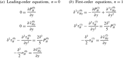
Bulk flow hydrodynamic equations for the symmetric and antisymmetric uniform heating of two plane walls at low frequency ratio, where
 ${\it\delta}^{2}\equiv -\text{i}{\it\beta}$
.
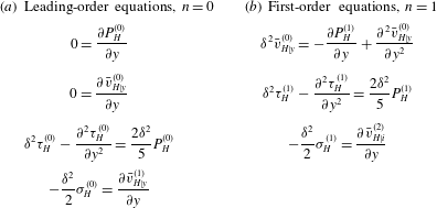
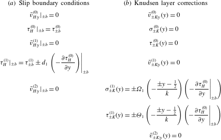
The Knudsen layer corrections for the local flow near any solid wall are denoted by a subscript ‘
 $K$
’, and have also been examined to
 $O(k^{2})$
. It has been shown that the well-known steady second-order tangential velocity slip model and Knudsen layer correction for a BGK gas are unaltered for unsteady flow at low frequency. This provides analytical justification for the application of the classical (steady) second-order slip condition to study unsteady flows. Importantly, all remaining slip boundary conditions and Knudsen layer corrections are modified at
 $O(k^{2})$
relative to the steady case; in particular, new terms arise to account for gas compressibility and temperature gradients near the wall. The leading-order effect of unsteadiness at low frequency in a slightly rarefied gas therefore occurs via a modification to the
 $O(k)$
bulk flow hydrodynamic equation, with a subset of the slip conditions and Knudsen layer corrections altered at
 $O(k^{2})$
.
We now present solutions for the unsteady uniform heating problem described in § 2. The hydrodynamic equations, velocity slip and temperature jump boundary conditions, and Knudsen layer corrections required to study the flow correct to first order in the scaled Knudsen number are summarised in tables 1 and 2. We apply the temperature jump coefficient
 $d_{1}=1.3027\ldots \,$
derived from the linearised Boltzmann–BGK equation by Sone (Reference Sone, Trilling and Wachman1969, Reference Sone and Dini1971) for a steady flow; as discussed in § 1, this coefficient was proven to remain unaltered by unsteady effects by Nassios & Sader (Reference Nassios and Sader2012) and Takata & Hattori (Reference Takata and Hattori2012). The Knudsen layer functions
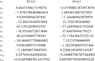
 ${\it\Omega}_{1}$
and
 ${\it\Theta}_{1}$
are defined in terms of the truncated series:
 $$\begin{eqnarray}{\it\Psi}({\it\eta})=\mathop{\sum }_{n=0}^{N}c_{n}J_{n}({\it\eta}),\end{eqnarray}$$
where
 ${\it\Psi}$
represents any of
 ${\it\Omega}_{1}$
and
 ${\it\Theta}_{1}$
. The required Knudsen layer coefficients are presented in Nassios & Sader (Reference Nassios and Sader2012); these coefficients are replicated in table 3 herein, with
 ${\it\delta}^{2}\equiv -\text{i}{\it\beta}$
.
Slip conditions and Knudsen layer corrections for the symmetric and antisymmetric uniform heating of two plane walls at low frequency ratio.

Coefficients of
 ${\it\Omega}_{1}({\it\eta})$
and
 ${\it\Theta}_{1}({\it\eta})$
, the Knudsen layer density functions.

The wall temperatures
 ${\it\tau}_{\pm b}^{(n)}$
for
 $n=0,1$
that appear in the slip conditions in table 2(a) are the
 $n$
th-order terms in the
 $k$
-expansion of
 ${\it\tau}_{\pm b}$
defined in (2.17). Using (4.2b
), we find:
 $$\begin{eqnarray}\displaystyle & \displaystyle {\it\tau}_{\pm b}^{(0)}={\it\upsilon}{\it\gamma}, & \displaystyle\end{eqnarray}$$
 $$\begin{eqnarray}\displaystyle & \displaystyle {\it\tau}_{\pm b}^{(n)}=0,\quad n\geqslant 1. & \displaystyle\end{eqnarray}$$
Next, we solve the system of differential equations in table 1 subject to the boundary conditions in table 2(a) and (4.4). Symmetric wall temperatures are assumed in § 4.1.1; see (4.4) with
 ${\it\upsilon}=+1$
at both walls.
As discussed in § 1, Manela & Hadjiconstantinou (Reference Manela and Hadjiconstantinou2010) studied the symmetric problem using the linearised Navier–Stokes–Fourier equations, with the classical (steady) first-order slip conditions derived by Sone (Reference Sone, Trilling and Wachman1969, Reference Sone and Dini1971, Reference Sone1974) applied at the walls. These boundary conditions are identical to those in table 2(a). However, the linearised Navier–Stokes–Fourier equations differ from those summarised in table 1 at
 $O(k)$
because the flow is non-isothermal. In § 4.1.1, we elucidate the effect of the modified hydrodynamic equations on the flow. The antisymmetric configuration is then considered in § 4.1.3, where
 ${\it\upsilon}=\pm 1$
at the upper and lower walls, i.e. at
 $y=\pm 1/2$
, respectively.
4.1.1 Symmetric wall temperatures
First, consider the leading-order equations in table 1(a). The first equation yields the hydrostatic pressure
 $$\begin{eqnarray}P_{H}^{(0)}=C_{\mathit{sym}},\end{eqnarray}$$
where
 $C_{\mathit{sym}}$
is a constant to be determined. From the second equation in table 1(a), the flow is incompressible at leading order and satisfies the no-slip boundary condition; see table 2(a). This gives zero mean wall-normal velocity, because the wall is stationary,
 $$\begin{eqnarray}\bar{v}_{H|y}^{(0)}=0.\end{eqnarray}$$
Therefore, no flow occurs in the continuum limit, i.e. for
 $k=0$
.
At leading order, the temperature of the gas matches the wall temperatures given by (4.4a
) with
 ${\it\upsilon}=+1$
; see table 2(a). The third equation in table 1(a) then yields the temperature in the gas at leading order. This is defined in terms of the hydrostatic pressure from (4.5):
 $$\begin{eqnarray}{\it\tau}_{H}^{(0)}=\left({\it\gamma}-\frac{2C_{\mathit{sym}}}{5}\right)\frac{\cosh ({\it\delta}y)}{\cosh \left({\displaystyle \frac{{\it\delta}}{2}}\right)}+\frac{2C_{\mathit{sym}}}{5}.\end{eqnarray}$$
Substituting (4.5) and (4.7) into the continuity equation in the fourth line of table 1(a) yields
 $$\begin{eqnarray}\frac{\partial \bar{v}_{H|y}^{(1)}}{\partial y}=\frac{{\it\delta}^{2}}{2}\left({\it\gamma}-\frac{2C_{\mathit{sym}}}{5}\right)\frac{\cosh ({\it\delta}y)}{\cosh \left({\displaystyle \frac{{\it\delta}}{2}}\right)}-\frac{3{\it\delta}^{2}}{10}C_{\mathit{sym}}.\end{eqnarray}$$
Equation (4.8) is a first-order differential equation for
 $\bar{v}_{H|y}^{(1)}$
, which must satisfy the no-penetration condition at both the upper and lower walls. The constant
 $C_{\mathit{sym}}$
therefore ensures the necessary degree of freedom exists in (4.8) to simultaneously satisfy no penetration at both walls. This establishes that mass conservation is the dominant physical mechanism driving the flow, which generates a hydrostatic pressure in the gas at leading order. This pressure is present across the full range of inertia, i.e. for all
 ${\it\beta}$
, which ensures the impermeability condition at the walls is satisfied.
In the symmetric case, the unique solution for
 $\bar{v}_{H|y}^{(1)}$
and
 $C_{\mathit{sym}}$
from (4.8) is
 $$\begin{eqnarray}\displaystyle & \displaystyle C_{\mathit{sym}}={\it\gamma}\frac{10\tanh \left({\displaystyle \frac{{\it\delta}}{2}}\right)}{3{\it\delta}+4\tanh \left({\displaystyle \frac{{\it\delta}}{2}}\right)}=P_{H}^{(0)}, & \displaystyle\end{eqnarray}$$
 $$\begin{eqnarray}\displaystyle & \displaystyle G_{\mathit{sym}}=0, & \displaystyle\end{eqnarray}$$
 $$\begin{eqnarray}\displaystyle & \displaystyle {\it\tau}_{H}^{(0)}={\it\gamma}\frac{3{\it\delta}\cosh ({\it\delta}y)+4\sinh \left({\displaystyle \frac{{\it\delta}}{2}}\right)}{3{\it\delta}\cosh \left({\displaystyle \frac{{\it\delta}}{2}}\right)}, & \displaystyle\end{eqnarray}$$
 $$\begin{eqnarray}\displaystyle & \displaystyle \bar{v}_{H|y}^{(1)}={\it\gamma}\frac{3{\it\delta}^{2}\left(\sinh ({\it\delta}y)-2y\sinh \left({\displaystyle \frac{{\it\delta}}{2}}\right)\right)}{6{\it\delta}\cosh \left({\displaystyle \frac{{\it\delta}}{2}}\right)+8\sinh \left({\displaystyle \frac{{\it\delta}}{2}}\right)}. & \displaystyle\end{eqnarray}$$
A similar procedure can be applied to solve the first order (
 $n=1$
) bulk flow quantities, using the equations in table 1(b). For brevity, we omit the derivation and summarise the unique solutions to
 $P_{H}^{(1)}$
,
 ${\it\tau}_{H}^{(1)}$
, and
 $\bar{v}_{H|y}^{(2)}$
,
 $$\begin{eqnarray}\displaystyle & \displaystyle P_{H}^{(1)}=-{\it\gamma}\frac{30{\it\delta}^{2}d_{1}\tanh ^{2}\left({\displaystyle \frac{{\it\delta}}{2}}\right)}{\left(3{\it\delta}+4\tanh \left({\displaystyle \frac{{\it\delta}}{2}}\right)\right)^{2}}, & \displaystyle\end{eqnarray}$$
 $$\begin{eqnarray}\displaystyle & \displaystyle {\it\tau}_{H}^{(1)}=-{\it\gamma}\frac{3{\it\delta}^{2}d_{1}\sinh \left({\displaystyle \frac{{\it\delta}}{2}}\right)\left(3{\it\delta}\cosh ({\it\delta}y)+4\sinh \left({\displaystyle \frac{{\it\delta}}{2}}\right)\right)}{\left(3{\it\delta}\cosh ({\it\delta}y)+4\sinh \left({\displaystyle \frac{{\it\delta}}{2}}\right)\right)^{2}}, & \displaystyle\end{eqnarray}$$
 $$\begin{eqnarray}\displaystyle & \displaystyle \bar{v}_{H|y}^{(2)}={\it\gamma}\frac{9{\it\delta}^{4}d_{1}\sinh \left({\displaystyle \frac{{\it\delta}}{2}}\right)\left(2y\sinh \left({\displaystyle \frac{{\it\delta}}{2}}\right)-\sinh ({\it\delta}y)\right)}{2\left(3{\it\delta}\cosh ({\it\delta}y)+4\sinh \left({\displaystyle \frac{{\it\delta}}{2}}\right)\right)^{2}}. & \displaystyle\end{eqnarray}$$
 $O(k)$
is achieved using the continuity equation in the third line of table 2(b). This yields an expression for the second order (
 $n=2$
) correction for the mean wall-normal velocity
 $\bar{v}_{H|y}^{(2)}$
.
4.1.2 Comparison with Manela & Hadjiconstantinou (Reference Manela and Hadjiconstantinou2010)
As discussed, the symmetric heating problem was previously studied by Manela & Hadjiconstantinou (Reference Manela and Hadjiconstantinou2010) using the linearised Navier–Stokes–Fourier equation. Interestingly, the
 $k$
-expansion of their solution (not shown here) yields algebraic expressions for the flow up to
 $O(k^{2})$
, which are identical to those reported in (4.9) and (4.10). However, the results in (4.9) and (4.10) are derived using the hydrodynamic equations in table 1, which differ from the linearised Navier–Stokes–Fourier equation. This is shown in (4.11), where we give the momentum conservation equations for the symmetric uniform heating problem, at both first and second order in
 $k$
, as formally derived from the Boltzmann–BGK equation,
 $$\begin{eqnarray}\displaystyle & \displaystyle {\it\delta}^{2}\bar{v}_{H|y}^{(1)}=-\frac{\partial P_{H}^{(2)}}{\partial y}+\frac{4}{3}\frac{\partial ^{2}\bar{v}_{H|y}^{(1)}}{\partial y^{2}}-\frac{2{\it\delta}^{2}}{3}\frac{\partial {\it\tau}_{H}^{(0)}}{\partial y}, & \displaystyle\end{eqnarray}$$
 $$\begin{eqnarray}\displaystyle & \displaystyle {\it\delta}^{2}\bar{v}_{H|y}^{(2)}=-\frac{\partial P_{H}^{(3)}}{\partial x_{y}}+\frac{4}{3}\frac{\partial ^{2}\bar{v}_{H|y}^{(2)}}{\partial y^{2}}-\frac{2{\it\delta}^{2}}{3}\frac{\partial {\it\tau}_{H}^{(1)}}{\partial y}. & \displaystyle\end{eqnarray}$$
 $O(k^{2})$
. As such, the linearised Navier–Stokes–Fourier equation and the equations in table 1 give identical results for the flow up to (i)
 $O(k)$
for the temperature and pressure and (ii)
 $O(k^{2})$
for the mean wall-normal velocity. This explains why the results of Manela & Hadjiconstantinou (Reference Manela and Hadjiconstantinou2010) are identical to those presented here, despite the use of different momentum transport equations. This is a unique property of the uniform heating problem. Indeed, it was shown by Nassios & Sader (Reference Nassios and Sader2012) that the additional body force term in the
 $O(k)$
momentum equation in table 1 is generally critical in determining the leading-order thermal creep flow for small
 ${\it\beta}$
– its inclusion will in general modify the velocity field.
4.1.3 Antisymmetric wall temperatures
We follow an identical approach to the one employed in § 4.1.1 to study the flow caused by antisymmetric heating; see (4.4), with
 ${\it\upsilon}=\pm 1$
. The leading order (
 $n=0$
) pressure, mean wall-normal velocity and temperature of the gas have the unique solutions:
 $$\begin{eqnarray}\displaystyle & \displaystyle P_{H}^{(0)}=C_{\mathit{asym}}, & \displaystyle\end{eqnarray}$$
 $$\begin{eqnarray}\displaystyle & \displaystyle \bar{v}_{H|y}^{(0)}=0, & \displaystyle\end{eqnarray}$$
 $$\begin{eqnarray}\displaystyle & \displaystyle {\it\tau}_{H}^{(0)}=\left({\it\gamma}-\frac{2C_{\mathit{asym}}}{5}\right)\frac{\sinh ({\it\delta}y)}{\sinh \left({\displaystyle \frac{{\it\delta}}{2}}\right)}+\frac{2C_{\mathit{asym}}}{5}. & \displaystyle\end{eqnarray}$$
 $k$
and the general solution for the first-order mean wall-normal velocity in terms of
 $C_{\mathit{asym}}$
is determined from the continuity equation
 $$\begin{eqnarray}\bar{v}_{H|y}^{(1)}=\frac{{\it\delta}}{2}\left({\it\gamma}-\frac{2C_{\mathit{asym}}}{5}\right)\frac{\cosh ({\it\delta}y)}{\cosh \left({\displaystyle \frac{{\it\delta}}{2}}\right)}+\frac{{\it\delta}^{2}C_{\mathit{asym}}y}{5}+G_{\mathit{asym}},\end{eqnarray}$$
where
 $G_{\mathit{asym}}$
is a constant of integration. Enforcing no penetration at both the upper and lower walls gives the unique solution for
 $\bar{v}_{y}^{(1)}$
,
 $$\begin{eqnarray}\displaystyle & \displaystyle C_{\mathit{asym}}=0=P_{H}^{(0)}, & \displaystyle\end{eqnarray}$$
 $$\begin{eqnarray}\displaystyle & \displaystyle G_{\mathit{asym}}=-{\it\gamma}\frac{{\it\delta}}{2\tanh \left({\displaystyle \frac{{\it\delta}}{2}}\right)}, & \displaystyle\end{eqnarray}$$
 $$\begin{eqnarray}\displaystyle & \displaystyle {\it\tau}_{H}^{(0)}={\it\gamma}\frac{\sinh ({\it\delta}y)}{\sinh \left({\displaystyle \frac{{\it\delta}}{2}}\right)}, & \displaystyle\end{eqnarray}$$
 $$\begin{eqnarray}\displaystyle & \displaystyle \bar{v}_{H|y}^{(1)}={\it\gamma}\frac{{\it\delta}\left(\cosh ({\it\delta}y)-\cosh \left({\displaystyle \frac{{\it\delta}}{2}}\right)\right)}{2\sinh \left({\displaystyle \frac{{\it\delta}}{2}}\right)}. & \displaystyle\end{eqnarray}$$
 $P_{H}^{(0)}=C_{\mathit{asym}}$
is therefore zero by symmetry from (4.13), i.e. the flow at leading order (
 $n=0$
) is isobaric. This contrasts markedly with the symmetric case, where the antisymmetric mean wall-normal velocity gives rise to a hydrostatic pressure; see (4.9).
Closure of this system to first order in
 $k$
yields the following expressions:
 $$\begin{eqnarray}\displaystyle & \displaystyle P_{H}^{(1)}=0, & \displaystyle\end{eqnarray}$$
 $$\begin{eqnarray}\displaystyle & \displaystyle {\it\tau}_{H}^{(1)}=-{\it\gamma}\frac{{\it\delta}d_{1}\sinh ({\it\delta}y)}{\tanh \left({\displaystyle \frac{{\it\delta}}{2}}\right)\sinh \left({\displaystyle \frac{{\it\delta}}{2}}\right)}, & \displaystyle\end{eqnarray}$$
 $$\begin{eqnarray}\displaystyle & \displaystyle \bar{v}_{H|y}^{(2)}={\it\gamma}\frac{{\it\delta}^{2}d_{1}\left(\cosh \left({\displaystyle \frac{{\it\delta}}{2}}\right)-\cosh ({\it\delta}y)\right)}{2\tanh \left({\displaystyle \frac{{\it\delta}}{2}}\right)\sinh \left({\displaystyle \frac{{\it\delta}}{2}}\right)}. & \displaystyle\end{eqnarray}$$
 $n=1$
) in
 $k$
is zero, which is in contrast to the symmetric case for the reasons discussed earlier.
4.2 High oscillation frequency,
${\it\theta}\gg 1$

In this section, we provide the complementary analysis to § 4.1 and explore the flow of a slightly rarefied gas when the oscillation frequency
 ${\it\omega}$
is much larger than the molecular collision frequency
 ${\it\nu}$
. This is achieved using the formalism in Nassios & Sader (Reference Nassios and Sader2013), which identified a local boundary layer flow near the wall that was distinct from the Knudsen layer; again a brief outline of the analysis is presented. A matched asymptotic expansion for the mass distribution function and its moments (
 ${\it\phi}$
,
 ${\it\sigma}$
,
 $\bar{v}$
,
 ${\it\tau}$
and
 $P$
, represented by
 ${\it\alpha}$
) is performed in the (small) inverse frequency ratio
 ${\it\theta}^{-1}$
:
 $$\begin{eqnarray}\displaystyle & \displaystyle {\it\alpha}={\it\alpha}_{H}+{\it\alpha}_{K}+{\it\alpha}_{C},\quad {\it\alpha}\in \{{\it\phi},{\it\sigma},\bar{v},{\it\tau}~\text{and}~P\}, & \displaystyle\end{eqnarray}$$
 $$\begin{eqnarray}\displaystyle & \displaystyle {\it\alpha}_{A}=\mathop{\sum }_{n=0}^{N}{\it\alpha}_{A}^{(n)}{\it\theta}^{-n},\quad A\in \{H,K,C\}. & \displaystyle\end{eqnarray}$$
 ${\it\theta}\gg 1$
is distinguished by a subscript
 $H$
and is studied using a classical Hilbert expansion in the (small) inverse frequency ratio
 ${\it\theta}^{-1}$
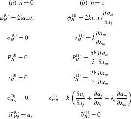
. The leading-order mass distribution function of the gas in the bulk flow region has been shown to be directly proportional to the applied oscillatory body force,
 $a_{i}$
. This yields a linearised Euler equation for the flow in that region to leading order in
 ${\it\theta}^{-1}$
; see table 4. Higher-order corrections to the mass distribution function in the expansion parameter
 ${\it\theta}^{-1}$
are proportional to gradients in the applied body force
 $a_{i}$
. The full set of hydrodynamic equations are summarised in table 4. Zero body force therefore yields no bulk flow. It has also been proven that the zero solution satisfies all Knudsen layer equations for
 $n\geqslant 0$
, i.e.
 $$\begin{eqnarray}{\it\alpha}_{K}^{(n)}=0.\end{eqnarray}$$
Outer flow field hydrodynamic relations to first order (
 $n=1$
) in the inverse frequency ratio
 ${\it\theta}^{-1}$
.

The local boundary layer flow near the wall (distinct from the Knudsen layer) is denoted by a subscript
 $C$
. The thickness of this boundary layer scales with the acoustic length scale
 $v_{mp}(T_{0})/{\it\omega}$
, which is much smaller than the gas mean free path
 ${\it\lambda}$
(which represents the thickness of the Knudsen layer) when the flow is highly oscillatory, i.e.
 ${\it\theta}\gg 1$
. The flow in the wall-normal direction within this boundary layer is thus collisionless to leading order. In contrast to the low-frequency case, explicit and general expressions are derived for the macroscopic flow quantities up to first order in
 ${\it\theta}^{-1}$
within the collisionless layer. This eliminates the need to solve a set of differential equations for the flow near a wall of arbitrary geometry. The collisionless layer equations are lengthy; for brevity, we do not summarise the full set of equations in this article and refer the reader to Nassios & Sader (Reference Nassios and Sader2013).
We apply this formalism to study high-frequency oscillatory uniform heating of two parallel plane walls; see figure 1. The (local) flows within the collisionless layers near each wall decouple because the body force vanishes, i.e.
 $a_{i}=0$
, and the bulk (Hilbert) flow is zero. Consequently, flows near each wall can be studied independently. We therefore consider the flow generated when an oscillatory temperature distribution of constant amplitude is imposed along a stationary, isolated plane wall; see figure 2. This flow is solved using the boundary conditions in (2.16) and the general formulae for the macroscopic flow quantities from Nassios & Sader (Reference Nassios and Sader2013). These formulae are given explicitly as functions of the
 $n$
th-order terms in the
 ${\it\theta}^{-1}$
-expansion of the velocity
 $V_{i}$
and temperature
 ${\it\tau}_{b}$
of the wall, as well as the reflected particle density
 ${\it\sigma}_{b}$
. All terms involving the applied body force
 $a_{i}$
are zero by (2.1a
), while the normal and geodesic curvatures are also zero because the wall is flat; see figure 2. The required expressions for the
 $n$
th-order terms in the
 ${\it\theta}^{-1}$
-expansion of the wall temperature from (2.17) are
 $$\begin{eqnarray}\displaystyle & \displaystyle {\it\tau}_{b}^{(0)}={\it\upsilon}{\it\gamma}, & \displaystyle\end{eqnarray}$$
 $$\begin{eqnarray}\displaystyle & \displaystyle {\it\tau}_{b}^{(n)}=0,\quad n\geqslant 1, & \displaystyle\end{eqnarray}$$
 $b$
’ denotes a quantity at the isolated wall,
 ${\it\upsilon}=\pm 1$
as before, and
 $a_{i}=0$
throughout the gas.
Schematic showing an infinite plane wall upon which a uniformly and harmonically varying temperature field is imposed. Dilute gas fills the half-space
 $y\geqslant 0$
.

The mean velocity of the wall
 $V_{i}$
is zero because the wall is stationary,
 $$\begin{eqnarray}V_{i}^{(n)}=0,\quad n\geqslant 0.\end{eqnarray}$$
The leading- and first-order terms in the
 ${\it\theta}^{-1}$
-expansion of the reflected particle density
 ${\it\sigma}_{b}$
from (2.16) are
 $$\begin{eqnarray}\displaystyle & \displaystyle {\it\sigma}_{b}^{(0)}=-\frac{{\it\tau}_{b}^{(0)}}{2}-2\sqrt{{\rm\pi}}\int _{-\infty }^{\infty }\int _{-\infty }^{\infty }\int _{-\infty }^{0}v_{y}\,{\it\phi}_{C|v_{y}<0}^{(0)}\,E(v_{x},v_{y},v_{z})\,\text{d}v_{y}\,\text{d}v_{x}\,\text{d}v_{z}, & \displaystyle\end{eqnarray}$$
 $$\begin{eqnarray}\displaystyle & \displaystyle {\it\sigma}_{b}^{(1)}=-2\sqrt{{\rm\pi}}\int _{-\infty }^{\infty }\int _{-\infty }^{\infty }\int _{-\infty }^{0}v_{y}\,{\it\phi}_{C|v_{y}<0}^{(1)}\,E(v_{x},v_{y},v_{z})\,\text{d}v_{y}\,\text{d}v_{x}\,\text{d}v_{z}, & \displaystyle\end{eqnarray}$$
 $E(v_{x},v_{y},v_{z})$
is defined in (2.13). Using (4.18) and (4.19) and the formulae in Nassios & Sader (Reference Nassios and Sader2013), (4.20) can be written in the following form
 $$\begin{eqnarray}\displaystyle & \displaystyle {\it\sigma}_{b}^{(0)}=-\frac{{\it\tau}_{b}^{(0)}}{2}, & \displaystyle\end{eqnarray}$$
 $$\begin{eqnarray}\displaystyle \displaystyle {\it\sigma}_{b}^{(1)} & = & \displaystyle \displaystyle -4\sqrt{{\rm\pi}}{\it\tau}_{b}^{(0)}\left(I_{3,1}(0)-I_{1,1}(0)+{\textstyle \frac{1}{3}}\left[I_{4,2}(0)-{\textstyle \frac{3}{2}}I_{2,2}(0)+{\textstyle \frac{3}{2}}I_{0,2}(0)\right.\right.\nonumber\\ \displaystyle & & \displaystyle \left.\!-\left.\!{\textstyle \frac{1}{2}}I_{4,0}(0)+{\textstyle \frac{9}{4}}I_{2,0}(0)-{\textstyle \frac{9}{4}}I_{0,0}(0)\right]\right),\end{eqnarray}$$
 $$\begin{eqnarray}I_{m,n}({\it\eta}_{C})=\frac{1}{{\rm\pi}}\left\{\begin{array}{@{}ll@{}}\displaystyle \int _{0}^{\infty }J_{m}(-\text{i}y_{0})J_{n}(-\text{i}|{\it\eta}_{C}-y_{0}|)\,\text{d}y_{0}, & n=2s+1,\\ \displaystyle \int _{0}^{\infty }\text{sgn}({\it\eta}_{C}-y_{0})J_{m}(-\text{i}y_{0})J_{n}(-\text{i}|{\it\eta}_{C}-y_{0}|)\,\text{d}y_{0}, & n=2s,\end{array}\right.\end{eqnarray}$$
with the indices
 $m,s\in \mathbb{Z}$
.
A full discussion of the integrals in (4.22) and their numerical treatment is provided in appendix 2 of Nassios & Sader (Reference Nassios and Sader2013). Equation (4.21) can then be related to the pressure of particles reflected from the wall using the ideal gas law defined in (2.12), i.e.
 $P_{b}^{(0)}={\it\sigma}_{0}^{(0)}+{\it\tau}_{b}^{(0)}$
and
 $P_{b}^{(1)}={\it\sigma}_{0}^{(1)}+{\it\tau}_{b}^{(1)}$
.
In § 4.2.1, we present the asymptotic solution correct to order
 $n=1$
in
 ${\it\theta}^{-1}$
for the isolated wall problem utilising the equations and formalism in Nassios & Sader (Reference Nassios and Sader2013), subject to the boundary conditions given in (4.18), (4.19) and (4.21). Importantly, (4.21) is defined in terms of the wall temperature
 ${\it\tau}_{b}^{(0)}$
and is equivalent to the corresponding expression for oscillatory thermal creep given in Nassios & Sader (Reference Nassios and Sader2013). We shall also discuss the implications of this in greater detail in § 4.2.1. This is followed in § 4.2.2 by a brief outline of the method required to construct the corresponding solutions for the macroscopic flow quantities in the two-wall case, for both symmetric and antisymmetric wall temperature distributions. In § 4.2.3 we contrast the results presented in §§ 4.2.1 and 4.2.2 with the work by Manela & Hadjiconstantinou (Reference Manela and Hadjiconstantinou2008), who studied the symmetric two-wall problem in a free molecular gas.
The hydrodynamic quantities,
 ${\it\sigma}$
,
 ${\it\tau}$
and
 $\bar{v}_{i}$
, at leading and first order in the inverse frequency ratio
 ${\it\theta}^{-1}$
, i.e.
 $n=0$
and
 $n=1$
, for oscillatory flow near a uniformly heated, stationary infinite plane wall. All functions take the implicit argument
 ${\it\eta}_{C}$
and are equivalent to the corresponding expressions for the oscillatory thermal creep problem in Nassios & Sader (Reference Nassios and Sader2013).

4.2.1 Solution for an isolated wall
The solution of an isolated wall is obtained by substituting (4.18), (4.19) and (4.21) into general formulae for the collisionless layer quantities presented in Nassios & Sader (Reference Nassios and Sader2013). This yields expressions for the density (
 ${\it\sigma}_{C}^{(0)}$
and
 ${\it\sigma}_{C}^{(1)}$
), mean wall-normal velocity (
 $\bar{v}_{C|y}^{(0)}$
and
 $\bar{v}_{C|y}^{(1)}$
) and the temperature (
 ${\it\tau}_{C}^{(0)}$
and
 ${\it\tau}_{C}^{(1)}$
) of the gas in terms of
 ${\it\tau}_{b}^{(0)}$
, which are summarised in table 5. Importantly, these formulae are identical to the corresponding expressions for oscillatory thermal creep, i.e. the flows in each case are identical functions of
 ${\it\tau}_{b}^{(0)}$
. This is a direct result of the explicit solvability property of the flow in this limit. The key point of difference between these two problems is the first-order mean tangential velocity, i.e.
 $\bar{v}_{H|x}^{(1)}$
, which is non-zero in the oscillatory thermal creep problem. As required, this thermal creep flow disappears in the uniform heating case, due to the absence of a temperature gradient along the wall, i.e.
 $\partial {\it\tau}_{b}^{(0)}/\partial x$
is zero; see (4.18). As before, the argument
 ${\it\eta}_{C}$
in table 5 is the wall-normal coordinate
 $y$
from figure 2, rescaled by the acoustic length scale
 $L_{c}=v_{mp}(T_{0})/{\it\omega}$
defined in (1.4).
4.2.2 Symmetric and antisymmetric cases
The solution for the two-wall problem depicted in figure 1 can be constructed from a translation and linear superposition of the isolated wall solutions (see figure 2 and table 5), as we now discuss. The boundary temperature field for the symmetric and antisymmetric two-wall problem is reported in (2.17); the
 ${\it\theta}^{-1}$
-expansion of (2.17) is
 $$\begin{eqnarray}\left.\begin{array}{@{}c@{}}{\it\tau}_{\pm b}^{(0)}={\it\upsilon}{\it\gamma},\quad {\it\upsilon}=\pm 1,\\ {\it\tau}_{\pm b}^{(1)}=0.\end{array}\right\}\end{eqnarray}$$
Next, we rescale the wall-normal coordinate
 ${\it\eta}_{C}$
by the geometric length scale, which is the distance between the walls
 $d$
; see figure 1. The new scaled normal coordinate is denoted as
 $y$
, and is related to
 ${\it\eta}_{C}$
by
 $$\begin{eqnarray}{\it\eta}_{C}=\frac{y}{\mathit{St}},\end{eqnarray}$$
where the
 $\mathit{St}={\it\omega}L/v_{mp}(T_{0})$
; see (1.5) and (2.6).
The temperature of the upper wall
 ${\it\tau}_{+b}^{(0)}$
is identical for both the symmetric and antisymmetric problems; see (4.23). To account for the flow at the upper wall in each case, the isolated wall solutions in table 5 are translated such that the wall located at
 ${\it\eta}_{C}=0$
is positioned at
 $y=1/2$
, while the wall temperature distribution
 ${\it\tau}_{b}^{(0)}$
is set in accord with the above discussion. A similar procedure can be applied at the lower wall (
 $y=-1/2$
), where
 ${\it\tau}_{-b}^{(0)}={\it\gamma}$
in the symmetric problem while
 ${\it\tau}_{-b}^{(0)}=-{\it\gamma}$
in the antisymmetric case. Using
 ${\it\alpha}$
to denote any of the macroscopic flow quantities
 ${\it\sigma}_{C}^{(n)}$
,
 $\bar{v}_{C|y}^{(n)}$
,
 ${\it\tau}_{C}^{(n)}$
and
 $P_{C}^{(n)}$
, the general solution for symmetric uniform heating of two walls is
 $$\begin{eqnarray}{\it\alpha}_{\mathit{sym}}(y)=\frac{1}{{\it\gamma}}\left[{\it\alpha}\left(\frac{{\textstyle \frac{1}{2}}-y}{\mathit{St}}\right)+{\it\alpha}\left(\frac{{\textstyle \frac{1}{2}}+y}{\mathit{St}}\right)\right],\end{eqnarray}$$
while the corresponding expression for antisymmetric heating is
 $$\begin{eqnarray}{\it\alpha}_{\mathit{asym}}(y,A)=\frac{1}{{\it\gamma}}\left[{\it\alpha}\left(\frac{{\textstyle \frac{1}{2}}-y}{\mathit{St}}\right)-{\it\alpha}\left(\frac{{\textstyle \frac{1}{2}}+y}{\mathit{St}}\right)\right].\end{eqnarray}$$
The two-wall solutions can be constructed by substituting the isolated wall expressions from table 5 into (4.25) and (4.26); for brevity, we omit the lengthy expressions that result.
4.2.3 Symmetric uniform heating by Manela & Hadjiconstantinou (Reference Manela and Hadjiconstantinou2008)
In addition to the (near continuum) low-frequency limit, Manela & Hadjiconstantinou (Reference Manela and Hadjiconstantinou2008) also studied the symmetric two-wall uniform heating problem for a free molecular gas, i.e.
 $k^{-1}\rightarrow 0$
. The collisionless Boltzmann equation was therefore considered, subject to the linearised diffuse reflection condition at both walls:
 $$\begin{eqnarray}-\text{i}\,\mathit{St}\,{\it\phi}+v_{y}\frac{\partial {\it\phi}}{\partial y}=0,\end{eqnarray}$$
where
 $\mathit{St}$
is the Strouhal number. The particle velocity
 $v_{y}$
has been scaled by the most probable speed at the equilibrium temperature of the gas
 $v_{mp}(T_{0})$
defined in (2.6), while the wall-normal coordinate
 $y$
has been scaled by the channel width
 $d$
. Integral equations for the macroscopic flow quantities were derived from (4.27), defined in terms of the Strouhal number and the reflected particle densities
 ${\it\sigma}_{\pm b}$
at the upper and lower walls. This was achieved using similar methods to those outlined in § 3.1.
The method of steepest descent was then applied to study the resulting integral equations for the density
 ${\it\sigma}$
, mean wall-normal velocity
 $\bar{v}_{y}$
and temperature
 ${\it\tau}$
derived from (4.27) for large Strouhal number, i.e.
 $\mathit{St}^{-1}\rightarrow 0$
. This yielded the closed form expressions for the reflected particle densities at both walls,
 $$\begin{eqnarray}{\it\sigma}_{\pm b}=-\frac{{\it\tau}_{\pm b}}{2},\end{eqnarray}$$
where
 ${\it\tau}_{\pm b}={\it\gamma}$
because the wall temperatures were assumed to be symmetric and
 ${\it\gamma}\equiv A/T_{0}$
is the normalised amplitude of the wall temperature. The reflected particle densities
 ${\it\sigma}_{\pm b}$
therefore decouple, which gives explicit formulae for the density, mean wall-normal velocity and temperature of the gas. Importantly, these formulae are identical to those constructed using (4.25) and the isolated wall solutions in table 5. Interestingly, despite the assumption of a free molecular gas, good agreement was observed between LVDSMC simulations of the flow and the analytical formulae for large Strouhal numbers and small Knudsen numbers, i.e.
 $\mathit{St}\gg 1$
and
 $k\ll 1$
.
We now discuss these observations in the context of the solution presented here, derived using the formalism in Nassios & Sader (Reference Nassios and Sader2013). Given that the frequency ratio
 ${\it\theta}$
can be expressed in terms of the Strouhal number (1.5), the limit
 $\mathit{St}^{-1}\rightarrow 0$
is equivalent to the high-frequency flow regime, i.e. where
 ${\it\theta}^{-1}\rightarrow 0$
. When
 ${\it\theta}\gg 1$
, gas particle advection parallel to a uniformly heated wall does not affect the flow, because the wall temperature is independent of the tangential coordinates
 $x$
and
 $z$
.
As discussed in Nassios & Sader (Reference Nassios and Sader2013), the scaled Knudsen number
 $k$
determines the strength of gas particle advection parallel to a solid wall. Since gas particles do not interact in the leading-order flow (i.e.
 ${\it\theta}^{-1}\rightarrow 0$
) generated by oscillatory uniform heating of two plane walls at high frequency for all
 $k$
, any effect of
 $k$
is eliminated. Consequently, (4.27) can be applied to study this flow.
However, collisional effects become important at higher order, and cannot be studied using the collisionless equation in (4.27). In this case, the asymptotic formulae derived in Nassios & Sader (Reference Nassios and Sader2013) and employed in this section provide a general framework with which to study flows for
 ${\it\theta}\gg 1$
and
 $k\ll 1$
up to
 $O({\it\theta}^{-1})$
. These higher-order asymptotic results account for the effect of collisions and advection along a solid wall, which are not captured by (4.27).
5 Results and discussion
Gas flows generated by the unsteady uniform heating problem are first studied using the asymptotic formulae for a lightly rarefied gas (
 $k\ll 1$
) in § 4. The primary aim is to use these formulae to elucidate the dominant physical mechanism driving the gas flow, in both the low- and high-frequency limits. The predictions of these formulae are then compared to direct numerical solutions that are valid for all frequencies and degrees of gas rarefaction, as specified in § 3.3 – this provides the first independent validation of the asymptotic theories of Nassios & Sader (Reference Nassios and Sader2012, Reference Nassios and Sader2013) and Takata et al. (Reference Takata, Aoki, Hattori and Hadjiconstantinou2012).
Asymptotic results in the low-frequency limit (
 ${\it\theta}\ll 1$
) are examined in § 5.1, with the symmetric and antisymmetric problems studied independently. The complementary high-frequency limit (
 ${\it\theta}\gg 1$
) is investigated in § 5.2. Because the flow is localised to collisionless boundary layers near the walls, we only study the related isolated wall problem; the relevant formulae are summarised in table 5. As we shall discuss, the unsteady uniform heating problem in the high-frequency limit yields a qualitative similarity to the oscillatory (time-varying) thermal creep problem considered in Nassios & Sader (Reference Nassios and Sader2013).
Due to inertia, the gas density, mean wall-normal velocity and temperature possess both real and imaginary components. Note the true (physical) solution of these time-varying flows are given by a weighted superposition between these real and imaginary components. For example, if the true temperature at the wall is
 $T_{\mathit{true}}=\text{Re}\{T\exp (-\text{i}{\it\omega}t)\}$
, then all true flow/temperature variables are given by
 $X_{\mathit{true}}=\text{Re}\{X\exp (-\text{i}{\it\omega}t)\}=\text{Re}\{X\}\cos ({\it\omega}t)-\text{Im}\{X\}\sin ({\it\omega}t)$
, for any variable
 $X$
. Thus, the solution periodically alternates between the real and imaginary components as time evolves.
In § 5.3, we explore the validity of the asymptotic formulae in § 4 by comparison with benchmark numerical solutions.
We remind the reader that the asymptotic solutions for the density and temperature for
 ${\it\theta}\ll 1$
are correct to
 $O(k)$
, while the mean wall-normal velocity is correct to
 $O(k^{2})$
. All hydrodynamic quantities for
 ${\it\theta}\gg 1$
are correct to
 $O({\it\theta}^{-1})$
.
5.1 Low oscillation frequency,
${\it\theta}\ll 1$

In this section, we use the asymptotic formulae of § 4.1 to study flow in the low oscillation frequency regime, i.e.
 ${\it\theta}\ll 1$
. Discussion of the symmetric problem is given in § 5.1.1, while the antisymmetric case is considered in § 5.1.2.
5.1.1 Symmetric wall temperatures
Since the gas flow is driven by temperature oscillations at the walls, we initially examine the temperature field as a function of the inertial parameter
 ${\it\beta}$
.
Temperature field. The real and imaginary components of the leading-order scaled temperature
 ${\it\tau}_{H}^{(0)}/{\it\gamma}$
from (4.9) are shown in figure 3, as a function of
 ${\it\beta}$
. Due to the no-slip condition inherent in the leading-order solution, the real and imaginary components of
 ${\it\tau}_{H}^{(0)}/{\it\gamma}$
at each wall are independent of
 ${\it\beta}$
, and equal to 1 and 0, respectively.
Scaled leading-order temperature of the symmetric problem:
 ${\it\tau}_{H}^{(0)}/{\it\gamma}$
. (a) Real component; (b) imaginary component. Results given for
 ${\it\beta}=1$
(small dashed),
 ${\it\beta}=10$
(medium dashed),
 ${\it\beta}=30$
(large dashed),
 ${\it\beta}=100$
(dot-dashed),
 ${\it\beta}=1000$
(dotted) and
 ${\it\beta}=10\,000$
(solid).

For zero inertia, i.e.
 ${\it\beta}=0$
, the expected steady solution is recovered, with constant and purely real gas temperature between the walls,
 $$\begin{eqnarray}{\it\tau}_{H|\mathit{sym}}^{(0)}={\it\gamma}.\end{eqnarray}$$
For non-zero but small inertia, i.e.
 ${\it\beta}\ll 1$
, a non-zero imaginary component arises, indicating a lag in the gas temperature response. The imaginary component increases in magnitude for small
 ${\it\beta}$
, attaining a peak value at
 $y=0$
for
 ${\it\beta}=13.6657\ldots \,$
before inflecting; see figure 3(b). For large inertia, i.e.
 ${\it\beta}\gg 1$
, thermal boundary layers form in both real and imaginary components near the walls; thermal gradients within these layers are large. Away from the walls, the temperature
 ${\it\tau}_{H}^{(0)}$
displays
 $1/\sqrt{{\it\beta}}$
decay throughout the bulk of the channel due to diffusive heat transport from the walls. This is evident from the small and large-
 ${\it\beta}$
asymptotic behaviour away from any walls:
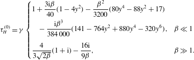 $$\begin{eqnarray}{\it\tau}_{H}^{(0)}={\it\gamma}\left\{\begin{array}{@{}ll@{}}\displaystyle 1+\frac{3\text{i}{\it\beta}}{40}(1-4y^{2})-\frac{{\it\beta}^{2}}{3200}(80y^{4}-88y^{2}+17) & \\ \displaystyle \quad -\,\frac{\text{i}{\it\beta}^{3}}{384\,000}(141-764y^{2}+880y^{4}-320y^{6}), & {\it\beta}\ll 1\\ \displaystyle \frac{4}{3\sqrt{2{\it\beta}}}(1+\text{i})-\frac{16\text{i}}{9{\it\beta}}, & {\it\beta}\gg 1.\end{array}\right.\end{eqnarray}$$
Thus, the temperature field exhibits spatial variations at finite inertia, which in principle can induce pressure and density variations in the gas – this coupling is now examined.
Pressure and density fields. The leading-order pressure,
 $P_{H}^{(0)}$
, i.e. which corresponds to the true pressure at zero frequency, is hydrostatic and non-zero; see (4.9). Operation at non-zero
 ${\it\beta}$
produces a deviation from this hydrostatic state, with the real and imaginary components of
 $P_{H}^{(0)}/{\it\gamma}$
for
 ${\it\beta}\in [0,1000]$
given in figure 4.
For zero inertia,
 ${\it\beta}=0$
, the pressure is identical to the temperature field
 ${\it\tau}_{H}^{(0)}/{\it\gamma}$
throughout the channel; see figure 4, where the real component is equal to
 $1$
and the imaginary component is zero. A lag in the pressure of the gas in response to the oscillatory wall temperatures arises for small
 ${\it\beta}$
. Interestingly, the imaginary component of
 $P_{H}^{(0)}/{\it\gamma}$
is non-monotonic in
 ${\it\beta}$
, whereas the real component is a monotonically decreasing function of
 ${\it\beta}$
. At
 ${\it\beta}=15.6470\ldots \,$
, the imaginary component attains its maximum value, and subsequently begins to decrease. For large
 ${\it\beta}$
, both real and imaginary components of the pressure again exhibit
 $1/\sqrt{{\it\beta}}$
decay, in line with the temperature field in (5.2) that is driving the pressure; the small- and large-
 ${\it\beta}$
asymptotics for the pressure are given by
 $$\begin{eqnarray}P_{H}^{(0)}={\it\gamma}\left\{\begin{array}{@{}ll@{}}\displaystyle 1+\frac{\text{i}{\it\beta}}{20}-\frac{{\it\beta}^{2}}{300}-\frac{23\text{i}{\it\beta}^{3}}{100\,800}, & {\it\beta}\ll 1\\ \displaystyle \frac{10}{3\sqrt{2{\it\beta}}}(1+\text{i})-\frac{40\text{i}}{9{\it\beta}}, & {\it\beta}\gg 1.\end{array}\right.\end{eqnarray}$$
The gas density is then determined from the ideal gas law in (4.8),
 $$\begin{eqnarray}{\it\sigma}_{H}^{(0)}=P_{H}^{(0)}-{\it\tau}_{H}^{(0)}.\end{eqnarray}$$
The small- and large-
 ${\it\beta}$
asymptotics of
 ${\it\sigma}_{H}^{(0)}$
(away from the walls) are:
 $$\begin{eqnarray}{\it\sigma}_{H}^{(0)}={\it\gamma}\left\{\begin{array}{@{}ll@{}}\displaystyle \frac{\text{i}{\it\beta}}{40}(12y^{2}-1)-\frac{{\it\beta}^{2}}{9600}(19-264y^{2}+240y^{4}) & \\ \displaystyle \quad -\,\frac{\text{i}{\it\beta}^{3}}{8\,064\,000}(-1121+16044y^{2}-18480y^{4}+6720y^{6}) & {\it\beta}\ll 1\\ \displaystyle \frac{10}{3\sqrt{2{\it\beta}}}(1+\text{i})-\frac{40\text{i}}{9{\it\beta}} & {\it\beta}\gg 1.\end{array}\right.\end{eqnarray}$$
Scaled leading-order hydrostatic pressure of the symmetric problem:
 $P_{H}^{(0)}/{\it\gamma}$
. (a) Real component; (b) imaginary component.

Plots of the real and imaginary components of
 ${\it\sigma}_{H}^{(0)}/{\it\gamma}$
are given in figure 5. For zero inertia,
 ${\it\sigma}_{H}^{(0)}=0$
throughout the channel; see the asymptotic formula for
 ${\it\beta}\ll 1$
in (5.5). For small
 ${\it\beta}$
, the imaginary (out-of-phase) component increases in magnitude, and is non-zero at the walls; the real component monotonically decreases towards the walls, for all
 ${\it\beta}$
. At the critical value of
 ${\it\beta}=15.6471\ldots \,$
, the imaginary component of
 ${\it\sigma}_{H}^{(0)}/{\it\gamma}$
attains its maximum value at the walls; at this
 ${\it\beta}$
the imaginary component of
 $P_{H}^{(0)}/{\it\gamma}$
is maximised. For
 ${\it\beta}\gg 1$
, the density exhibits
 $1/\sqrt{{\it\beta}}$
decay away from the walls, as expected; see (5.5). At the walls, the real component of
 ${\it\sigma}_{H}^{(0)}/{\it\gamma}$
asymptotes to 1 with increasing
 ${\it\beta}$
, because
 $P_{H}^{(0)}/{\it\gamma}$
decays to 0; see figures 4(a) and 5(b).
With the temperature, pressure and density fields determined, we now turn our attention to their effect on the velocity field (our primary goal).
Scaled leading-order density of the symmetric problem:
 ${\it\sigma}_{H}^{(0)}/{\it\gamma}$
. (a) Real component; (b) imaginary component. Results given for
 ${\it\beta}=1$
(small dashed),
 ${\it\beta}=15.6471$
(medium dashed),
 ${\it\beta}=30$
(large dashed),
 ${\it\beta}=100$
(dot-dashed),
 ${\it\beta}=1000$
(dotted) and
 ${\it\beta}=10\,000$
(solid).

Mean wall-normal velocity. We now study the first-order (
 $n=1$
) component of the mean flow,
 $\bar{v}_{H|y}^{(1)}$
(see (4.9)), because the
 $n=0$
term is zero – the component
 $\bar{v}_{H|y}^{(1)}$
thus specifies the leading-order behaviour of the velocity field. To facilitate discussion, we calculate an average spatial velocity in the gas. The velocity is antisymmetric in
 $y$
, and we therefore calculate the average wall-normal velocity
 $u_{y}^{(1)}$
in the upper half-channel,
 $0\leqslant y\leqslant 1/2$
:
 $$\begin{eqnarray}u_{y}^{(1)}=2\int _{0}^{1/2}\bar{v}_{H|y}^{(1)}\,\text{d}y=-\frac{3{\it\delta}{\it\gamma}}{4}\frac{4-4\cosh \left({\displaystyle \frac{{\it\delta}}{2}}\right)+{\it\delta}\sinh \left({\displaystyle \frac{{\it\delta}}{2}}\right)}{3{\it\delta}\cosh \left({\displaystyle \frac{{\it\delta}}{2}}\right)+4\sinh \left({\displaystyle \frac{{\it\delta}}{2}}\right)}.\end{eqnarray}$$
The asymptotic behaviour of this average wall-normal velocity, for small and large
 ${\it\beta}$
(away from the walls), is
 $$\begin{eqnarray}u_{y}^{(1)}={\it\gamma}\left\{\begin{array}{@{}ll@{}}\displaystyle \frac{{\it\beta}^{2}}{640}+\frac{3\text{i}{\it\beta}^{3}}{25\,600}, & {\it\beta}\ll 1\\ \displaystyle \frac{1}{4}\sqrt{\frac{{\it\beta}}{2}}(1-\text{i})+\frac{4}{3}, & {\it\beta}\gg 1.\end{array}\right.\end{eqnarray}$$
We consider four separate limits: (i) zero inertia,
 ${\it\beta}=0$
; (ii) small inertia,
 ${\it\beta}\ll 1$
; (iii) intermediate inertia,
 ${\it\beta}\sim O(1)$
; and (iv) large inertia,
 ${\it\beta}\gg 1$
.
Zero inertia (
 ${\it\beta}=0$
). The flow is steady and incompressible; see the continuity equation in the last line of table 1(a). As such, the mean wall-normal velocity,
 $\bar{v}_{H|y}^{(1)}$
, is zero throughout the gas.
Small inertia (
 ${\it\beta}\ll 1$
). For small inertia, the leading-order density
 ${\it\sigma}_{C}^{(0)}$
is of
 $O({\it\beta})$
and varies quadratically in the normal coordinate,
 $y$
; see the
 ${\it\beta}\ll 1$
asymptotic in (5.5). The gas density is therefore out of phase with the wall temperature oscillations. By the continuity equation (mass conservation), this drives a compressible flow that is both (i) in-phase with the wall temperature oscillations, and (ii) antisymmetric in the wall-normal coordinate
 $y$
; see figure 6(a) for
 ${\it\beta}=10^{-4}$
, and the
 ${\it\beta}\ll 1$
asymptotic in (5.7). As
 ${\it\beta}$
increases, an additional out-of-phase correction to
 $\bar{v}_{H|y}^{(1)}$
arises due to the
 $O({\it\beta}^{2})$
term in the density; see figure 6(b) for
 ${\it\beta}=10^{-4}$
and (5.7).
Scaled first-order mean wall-normal velocity of symmetric problem:
 $\bar{v}_{H|y}^{(1)}/({\it\beta}^{l}{\it\gamma})$
, where
 $l$
is chosen to match dominant asymptotic behaviour in
 ${\it\beta}$
. Real, (
 $l=2$
), imaginary (
 $l=3$
). (a) Real component; (b) imaginary component. Results given for
 ${\it\beta}=10^{-4}$
(small dashed),
 ${\it\beta}=10^{-2}$
(small dashed),
 ${\it\beta}=10$
(large dashed),
 ${\it\beta}=15.647$
(dot-dashed),
 ${\it\beta}=30$
(dotted) and
 ${\it\beta}=50.4757$
(solid). Note that results for
 ${\it\beta}=10^{-4}$
and
 ${\it\beta}=10^{-2}$
are indistinguishable on the graph.

Intermediate inertia (
 ${\it\beta}\sim O(1)$
). For intermediate inertia, the imaginary component of
 ${\it\sigma}_{H}^{(0)}$
is positive at the walls,
 $y=\pm 1/2$
. In contrast, the density throughout the bulk of the channel is otherwise negative. As discussed, for
 ${\it\beta}=15.6471\ldots \,$
the imaginary component of the gas density attains its maximum value at the walls, and begins to decrease with further increases in
 ${\it\beta}$
. This causes a similar inflection in the real component of the average velocity in the upper half-channel,
 $u_{y}^{(1)}$
, where the maximum in the real part of the average normal velocity,
 $u_{y}^{(1)}$
, in (5.6) occurs for
 $$\begin{eqnarray}{\it\beta}={\it\beta}_{c}=22.5002\ldots .\end{eqnarray}$$
For
 ${\it\beta}>{\it\beta}_{c}$
, the real and imaginary components of
 $u_{y}^{(1)}$
are monotonically decreasing functions of
 ${\it\beta}$
. This causes a flow reversal in the real component of
 $\bar{v}_{H|y}^{(1)}$
, which occurs at
 ${\it\beta}=50.4757\ldots ;$
the onset of this reversal is illustrated by plots of the real component of
 $\bar{v}_{H|y}^{(1)}$
from
 ${\it\beta}=10$
to
 ${\it\beta}=50.4757$
, which are given in figure 6(a). No reversal occurs in the imaginary component of
 $\bar{v}_{H|y}^{(1)}$
, because it is a monotonically decreasing function of
 ${\it\beta}$
, for all
 ${\it\beta}$
.
Large inertia (
 ${\it\beta}\gg 1$
). In the limit of large inertia, the temperature and density fields are confined to thin boundary layers near the walls, and the hydrostatic pressure decays to zero; see the
 ${\it\beta}\gg 1$
asymptotics in (5.2), (5.3) and (5.5). Away from the walls, the real and imaginary components of
 ${\it\sigma}_{H}^{(0)}$
are therefore independent of
 $y$
; see figure 5. From the continuity equation, a suitable choice of scale for
 $\bar{v}_{H|y}^{(1)}$
then yields a linear velocity profile away from the walls that is evident in figure 7; see
 ${\it\beta}=1000$
and
 ${\it\beta}=10\,000$
. This contrasts with the near-wall velocity profile, which exhibits strong gradients.
Scaled first-order mean wall-normal velocity of symmetric problem:
 $\bar{v}_{H|y}^{(1)}/(\sqrt{{\it\beta}}{\it\gamma})$
. (a) Real component; (b) imaginary component. Results given for
 ${\it\beta}=10$
(medium dashed),
 ${\it\beta}=50.4757$
(large dashed),
 ${\it\beta}=100$
(dot-dashed) and
 ${\it\beta}=1000$
(dotted) and
 ${\it\beta}=10\,000$
(solid).

Summary. This analysis establishes the overriding physical mechanism driving gas flow in this problem: finite density variations at continuum order,
 $O(1)$
, induced by temperature and pressure variations of the same order (via the ideal gas law), and mass conservation. Note that this non-continuum
 $O(k)$
velocity field is driven by continuum-order effects in the temperature and pressure, as dictated by the asymptotic theory. Momentum transport does not play a role in driving this non-continuum flow.
5.1.2 Antisymmetric wall temperatures
We now provide an analogous (and abbreviated) discussion for the problem where the wall temperatures are antisymmetric, i.e. they are equal in magnitude but opposite in sign.
Temperature field. Plots of the real and imaginary components of the scaled temperature
 ${\it\tau}_{H}^{(0)}/{\it\gamma}$
from (4.9) are given in figure 8. As for the symmetric case, a steady (purely real) temperature profile is recovered for zero inertia, i.e.
 ${\it\beta}=0$
,
 $$\begin{eqnarray}{\it\tau}_{H|\mathit{asym}}^{(0)}=2{\it\gamma}y.\end{eqnarray}$$
A phase lag in the gas temperature field occurs as
 ${\it\beta}$
increases, and thermal boundary layers form near the walls for large inertia, i.e.
 ${\it\beta}\gg 1$
; see figure 8 for
 ${\it\beta}=1000$
and
 ${\it\beta}=10\,000$
.
Scaled leading-order temperature of antisymmetric problem:
 ${\it\tau}_{H}^{(0)}/{\it\gamma}$
. (a) Real component; (b) imaginary component; (c) magnitude. Results given for
 ${\it\beta}=1$
(small dashed),
 ${\it\beta}=10$
(medium dashed),
 ${\it\beta}=30$
(large dashed),
 ${\it\beta}=100$
(dot-dashed),
 ${\it\beta}=1000$
(dotted) and
 ${\it\beta}=10\,000$
(solid).

Density field. As discussed in § 4.1.3, the hydrostatic pressure at leading order (
 $n=0$
) is zero for the antisymmetric case, which contrasts with the symmetric problem; see (4.14). From the ideal gas law in (4.8), the gas density is thus:
 $$\begin{eqnarray}{\it\sigma}_{H}^{(0)}=-{\it\tau}_{H}^{(0)}.\end{eqnarray}$$
Substituting (5.10) into the continuity equation in the final line of table 1, we thus find that gradients in the mean wall-normal velocity are caused solely by the temperature field of the gas; this contrasts strongly with the symmetric case, where gas density is controlled by both the temperature and pressure.
We now use this observation to study the first-order mean wall-normal velocity,
 $\bar{v}_{H|y}^{(1)}$
, which is the leading-order mean flow (as for the symmetric problem).
Mean wall-normal velocity. We again calculate the average velocity in the upper half-channel,
 $$\begin{eqnarray}u_{y}^{(1)}=2\int _{0}^{1/2}\bar{v}_{H|y}^{(1)}\,\text{d}y={\it\gamma}\left[1-\frac{{\it\delta}}{2}\coth \left(\frac{{\it\delta}}{2}\right)\right].\end{eqnarray}$$
The corresponding small- and large-
 ${\it\beta}$
asymptotic results are
 $$\begin{eqnarray}\displaystyle u_{y}^{(1)}={\it\gamma}\left\{\begin{array}{@{}ll@{}}\displaystyle \frac{\text{i}{\it\beta}}{12}-\frac{{\it\beta}^{2}}{720}-\frac{\text{i}{\it\beta}^{3}}{30\,240}, & {\it\beta}\ll 1\\ \displaystyle 1+\sqrt{\frac{{\it\beta}}{2}}(\text{i}-1), & {\it\beta}\gg 1.\end{array}\right.\end{eqnarray}$$
These formulae are again used in conjunction with the temperature field,
 ${\it\tau}_{H}^{(0)}$
, to study
 $\bar{v}_{H|y}^{(1)}$
across the full range of inertia,
 ${\it\beta}$
.
Zero inertia (
 ${\it\beta}=0$
). Again, no flow is generated in the steady limit.
Small inertia (
 ${\it\beta}\ll 1$
). For small and non-zero inertia, the steady and purely real component for the temperature
 ${\it\tau}_{H|\mathit{asym}}^{(0)}$
drives a compressible (out-of-phase) mean flow via mass conservation; see asymptotics for
 ${\it\beta}\ll 1$
in (5.12), and plots of the scaled mean wall-normal flow profile in the upper half-channel,
 $0\leqslant y\leqslant 1/2$
, given in figure 9. The real component of the temperature field,
 ${\it\tau}_{H}^{(0)}$
, is monotonically increasing in
 $y$
for small
 ${\it\beta}$
; see figure 8, with
 ${\it\beta}=1$
.
Scaled first-order mean wall-normal velocity of antisymmetric problem:
 $\bar{v}_{H|y}^{(1)}/({\it\beta}^{l}{\it\gamma})$
, where
 $l$
is chosen to match the dominant asymptotic behaviour in
 ${\it\beta}$
. (a) Real (
 $l=2$
); (b) imaginary (
 $l=1$
). Results given for
 ${\it\beta}=10^{-4}$
(small dashed),
 ${\it\beta}=10$
(large dashed),
 ${\it\beta}=30$
(dot-dashed) and
 ${\it\beta}=50$
(solid).

Scaled first-order mean wall-normal velocity of antisymmetric problem:
 $\bar{v}_{H|y}^{(1)}/(\sqrt{{\it\beta}}{\it\gamma})$
. (a) Real component; (b) imaginary component. Results given for
 ${\it\beta}=10$
(medium dashed),
 ${\it\beta}=50$
(large dashed),
 ${\it\beta}=100$
(dot-dashed) and
 ${\it\beta}=1000$
(dotted) and
 ${\it\beta}=10\,000$
(solid).

From the continuity equation in table 1(a), and (5.10), the imaginary component of
 $\bar{v}_{H|y}^{(1)}$
is therefore monotonically decreasing in
 $y$
. Together with the no-penetration condition at the walls, this causes the inverted parabolic flow profile in figure 9(b) for
 ${\it\beta}=10^{-4}$
.
The real component of
 $\bar{v}_{H|y}^{(1)}$
is driven by the
 $O({\it\beta})$
correction to
 ${\it\tau}_{H}^{(0)}$
for small inertia, which is zero at (i) the centre of the channel and (ii) the upper wall. Once more, from the continuity equation and (5.10), this explains the inflected flow profile in the real component of
 $\bar{v}_{H|y}^{(1)}$
for
 ${\it\beta}=10^{-4}$
; see figure 9(a). The magnitude of both the real and imaginary component of
 $\bar{v}_{H|y}^{(1)}$
are also increasing functions of
 ${\it\beta}$
at small inertia; this is evident from plots of the scaled profiles in figure 9 for
 ${\it\beta}=10^{-4}$
and
 ${\it\beta}=10^{-2}$
.
Intermediate inertia (
 ${\it\beta}\sim O(1)$
). As
 ${\it\beta}$
is increased further, the magnitude of
 $\bar{v}_{H|y}^{(1)}$
continues to increase. Both components of the mean wall-normal velocity
 $\bar{v}_{H|y}^{(1)}$
therefore display identical behaviour to that established for small inertia; see figures 9 and 10 for
 ${\it\beta}=10$
,
 ${\it\beta}=30$
and
 ${\it\beta}=50$
.
High inertia (
 ${\it\beta}\gg 1$
). Contrasting behaviour to the symmetric problem is observed at high inertia. As for the symmetric case, perturbations to the temperature,
 ${\it\tau}_{H}^{(0)}$
, are confined to boundary layers near the walls, with exponential decay exhibited in the (scaled) normal coordinate,
 $y$
, away from the walls; see figure 8 for
 ${\it\beta}=1000$
and
 ${\it\beta}=10\,000$
. However,
 $P_{H}^{(0)}=0$
here; hence, by continuity and (5.10), flow throughout the bulk of the channel (away from any walls) is divergence free (incompressible), and the mean wall-normal velocity outside the boundary layers is thus independent of
 $y$
; see figure 10. Within the boundary layers near the walls, gradients in the temperature field are large. This drives similarly large gradients in the scaled mean wall-normal velocity near the walls; see plots of the scaled mean wall-normal velocity in figure 10 for
 ${\it\beta}=1000$
and
 ${\it\beta}=10\,000$
.
Scaled temperature,
 ${\it\tau}_{C}^{(0)}/{\it\tau}_{b}^{(0)}$
and
 ${\it\tau}_{C}^{(1)}/{\it\tau}_{b}^{(0)}$
: (a) Real; (b) imaginary. Results given for the leading-order solution (
 $n=0$
, solid) and first-order correction (
 $n=1$
, dashed). Numerical data for the imaginary components in figures 11–15 are affected by round-off error (noise) due to integrable singularities in the integrands. This could not be suppressed with available computational resources and was smoothed using a polynomial regression fit of order 50; the coefficients were determined using ordinary least squares. This does not affect the shape of the presented curves however suppresses the numerical noise.

Summary. This analysis shows that the mechanisms driving gas flow in the antisymmetric problem differ to those of the symmetric problem: pressure no longer has an effect here, with density variations being driven purely by temperature variations and mass conservation. Momentum transport again does not play a role.
5.2 High oscillation frequency,
${\it\theta}\gg 1$

In this section, we examine the high-frequency limit,
 ${\it\theta}\gg 1$
, for infinitesimally small Knudsen number,
 $k\ll 1$
, in accord with the asymptotic theory of Nassios & Sader (Reference Nassios and Sader2013). As discussed in § 4.2.1, formulae for the zeroth- and first-order scaled densities (
 ${\it\sigma}_{C}^{(0)}/{\it\tau}_{b}^{(0)}$
and
 ${\it\sigma}_{C}^{(1)}/{\it\tau}_{b}^{(0)}$
), mean wall-normal velocities (
 $\bar{v}_{C|y}^{(0)}/{\it\tau}_{b}^{(0)}$
and
 $\bar{v}_{C|y}^{(1)}/{\it\tau}_{b}^{(0)}$
) and temperatures (
 ${\it\tau}_{C}^{(0)}/{\it\tau}_{b}^{(0)}$
and
 ${\it\tau}_{C}^{(1)}/{\it\tau}_{b}^{(0)}$
) for the uniform heating problem (in table 5), are identical to corresponding expressions for the oscillatory thermal creep problem. We remind the reader that the leading-order term in the
 ${\it\theta}^{-1}$
-expansion of the wall temperature,
 ${\it\tau}_{b}^{(0)}$
, is defined in (4.18). Consequently, key features of the temperature and density at both zeroth- and first-order in
 ${\it\theta}^{-1}$
have already been described in Nassios & Sader (Reference Nassios and Sader2013), where the oscillatory thermal creep flow was studied in detail for
 ${\it\theta}\gg 1$
and
 $k\ll 1$
. Plots of the scaled temperature and density are given in figures 11 and 12, respectively. The mean wall-normal velocity at both orders was also examined in Nassios & Sader (Reference Nassios and Sader2013), plots of which are given in figure 13. In this section, we provide a summary of the key features of the flow that were discussed in Nassios & Sader (Reference Nassios and Sader2013), for completeness.
Scaled density,
 ${\it\sigma}_{C}^{(0)}/{\it\tau}_{b}^{(0)}$
and
 ${\it\sigma}_{C}^{(1)}/{\it\tau}_{b}^{(0)}$
: (a) Real; (b) imaginary. Results given for the leading-order solution (
 $n=0$
, solid) and first-order correction (
 $n=1$
, dashed).

Scaled mean normal velocity,
 $\bar{v}_{C|y}^{(0)}/x$
and
 $\bar{v}_{C|y}^{(1)}/x$
: (a) Real; (b) imaginary. Results given for the leading-order solution (
 $n=0$
, solid) and first-order correction (
 $n=1$
, dashed).

To begin, consider the real component of the leading order (
 $n=0$
) scaled temperature in figure 11(a). At the wall (
 ${\it\eta}_{C}=0$
),
 ${\it\tau}_{C}^{(0)}/({\it\upsilon}{\it\gamma})=1/2$
whereas the scaled wall temperature is
 ${\it\tau}_{b}^{(0)}/({\it\upsilon}{\it\gamma})=1$
; see (4.18). Therefore there is a jump in the real component of the temperature at the wall to leading order in
 ${\it\theta}^{-1}$
. However, the imaginary component does not exhibit a jump at this order; see figure 11(b). In contrast, the imaginary component of the first-order scaled temperature is non-zero at the wall, while the real component at this order is zero. From linearity, the flow at
 $O({\it\theta}^{-1})$
can be written as the sum of a free molecular and collisional contribution:
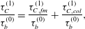 $$\begin{eqnarray}\frac{{\it\tau}_{C}^{(1)}}{{\it\tau}_{b}^{(0)}}=\frac{{\it\tau}_{C,\mathit{fm}}^{(1)}}{{\it\tau}_{b}^{(0)}}+\frac{{\it\tau}_{C,\mathit{col}}^{(1)}}{{\it\tau}_{b}^{(0)}},\end{eqnarray}$$
where
 $$\begin{eqnarray}\displaystyle \displaystyle \frac{{\it\tau}_{C,\mathit{fm}}^{(1)}}{{\it\tau}_{b}^{(0)}} & = & \displaystyle \displaystyle -\frac{8}{3{\rm\pi}}\left(J_{2}(-\text{i}{\it\eta}_{C})-\frac{1}{2}J_{0}(-\text{i}{\it\eta}_{C})\right)\left(\vphantom{\left[\frac{9}{4}\right]}I_{3,1}(0)-I_{1,1}(0)\right.\nonumber\\ \displaystyle & & \displaystyle \displaystyle +\left.\frac{1}{3}\left[I_{4,2}(0)-\frac{3}{2}I_{2,2}(0)+\frac{3}{2}I_{0,2}(0)-\frac{1}{2}I_{4,0}(0)+\frac{9}{4}I_{2,0}(0)-\frac{9}{4}I_{0,0}(0)\right]\right),\nonumber\\ \displaystyle & & \displaystyle\end{eqnarray}$$
 $$\begin{eqnarray}\displaystyle \displaystyle \frac{{\it\tau}_{C,\mathit{col}}^{(1)}}{{\it\tau}_{b}^{(0)}} & = & \displaystyle \frac{4}{3{\rm\pi}}\left[\left[I_{3,2}({\it\eta}_{C})-I_{1,2}({\it\eta}_{C})-\frac{1}{2}I_{3,0}({\it\eta}_{C})+\frac{1}{2}I_{1,0}({\it\eta}_{C})\right]\right.\nonumber\\ \displaystyle & & \displaystyle +\,\frac{1}{3}\left[\vphantom{\frac{21}{8}}I_{4,3}({\it\eta}_{C})-\frac{3}{2}I_{2,3}({\it\eta}_{C})+\frac{3}{2}I_{0,3}({\it\eta}_{C})-I_{4,1}({\it\eta}_{C})+3I_{2,1}({\it\eta}_{C})\right.\nonumber\\ \displaystyle & & \displaystyle \displaystyle -\left.\!\left.\!3I_{0,1}({\it\eta}_{C})+\frac{5}{4}I_{4,-1}({\it\eta}_{C})-\frac{21}{8}I_{2,-1}({\it\eta}_{C})+\frac{21}{8}I_{0,-1}({\it\eta}_{C})\right]\right]\nonumber\\ \displaystyle & & \displaystyle -\,\frac{2}{3}\frac{{\it\eta}_{C}}{\sqrt{{\rm\pi}}}\left[J_{3}(-\text{i}{\it\eta}_{C})-\frac{3}{2}J_{1}(-\text{i}{\it\eta}_{C})+\frac{3}{2}J_{-1}(-\text{i}{\it\eta}_{C})\right].\end{eqnarray}$$
 ${\it\theta}^{-1}\rightarrow 0$
, there is no collisional contribution and flow in the wall-normal direction is free molecular. From figures 14(b,d), the jump in the imaginary component of the temperature at first order is caused by collisional effects near the wall, which dominate free molecular contributions of this order throughout the gas. A jump in the scaled temperature of the gas relative to the temperature of the wall is thus evident for all time; this jump alternates between a zeroth- and first-order effect in the inverse frequency ratio
 ${\it\theta}^{-1}$
. A similar analysis of the scaled density in figure 12 yields identical conclusions.
The free molecular and collisional components of the first-order scaled temperature,
 ${\it\tau}_{C}^{(1)}/{\it\tau}_{b}^{(0)}$
. Free molecular component: (a) real; (b) imaginary. Collisional component: (c) real; (d) imaginary.

The free molecular and collisional components of the first-order scaled mean normal velocity,
 $\bar{v}_{C|y}^{(1)}/{\it\tau}_{b}^{(0)}$
. Free molecular component: (a) real; (b) imaginary. Collisional component: (c) real; (d) imaginary.

As required for a solid wall, the real and imaginary components of the scaled mean wall-normal velocity satisfy the no-penetration condition; see figure 13. As distinct from the oscillatory thermal creep problem, both the scaled and unscaled mean wall-normal velocities are independent of the tangential coordinate
 $x$
because the boundary temperature distribution is uniform; see (4.18). In line with our findings for the scaled temperature and density, by linearity the flow at
 $O({\it\theta}^{-1})$
can be written as the sum of a free molecular and collisional contribution:
 $$\begin{eqnarray}\frac{\bar{v}_{C|y}^{(1)}}{x}=\frac{\bar{v}_{C|y,\mathit{fm}}^{(1)}}{{\it\tau}_{b}^{(0)}}+\frac{\bar{v}_{C|y,\mathit{col}}^{(1)}}{{\it\tau}_{b}^{(0)}},\end{eqnarray}$$
where
 $$\begin{eqnarray}\displaystyle \displaystyle \frac{\bar{v}_{C|y,\mathit{fm}}^{(1)}}{{\it\tau}_{b}^{(0)}} & = & \displaystyle \displaystyle -\frac{4}{{\rm\pi}}J_{1}(-\text{i}{\it\eta}_{C})\left(I_{3,1}(0)-I_{1,1}(0)+\frac{1}{3}\left[I_{4,2}(0)-\frac{3}{2}I_{2,2}(0)+\frac{3}{2}I_{0,2}(0)\right.\right.\nonumber\\ \displaystyle & & \displaystyle \displaystyle -\left.\!\left.\!\frac{1}{2}I_{4,0}(0)+\frac{9}{4}I_{2,0}(0)-\frac{9}{4}I_{0,0}(0)\right]\right),\end{eqnarray}$$
 $$\begin{eqnarray}\displaystyle \frac{\bar{v}_{C|y,\mathit{col}}^{(1)}}{{\it\tau}_{b}^{(0)}} & = & \displaystyle \frac{2}{{\rm\pi}}\left([I_{3,1}({\it\eta}_{C})-I_{1,1}({\it\eta}_{C})]+\frac{1}{3}\left[I_{4,2}({\it\eta}_{C})-\frac{3}{2}I_{2,2}({\it\eta}_{C})+\frac{3}{2}I_{0,2}({\it\eta}_{C})\right.\right.\nonumber\\ \displaystyle & & \displaystyle -\left.\!\left.\!\frac{1}{2}I_{4,0}({\it\eta}_{C})+\frac{9}{4}I_{2,0}({\it\eta}_{C})-\frac{9}{4}I_{0,0}({\it\eta}_{C})\right]\right)-\frac{{\it\eta}_{C}}{\sqrt{{\rm\pi}}}[J_{2}(-\text{i}{\it\eta}_{C})-J_{0}(-\text{i}{\it\eta}_{C})].\nonumber\\ \displaystyle & & \displaystyle\end{eqnarray}$$
 $O({\it\theta}^{-1})$
dominates the corresponding free molecular contribution; see figures 15(a,c). Contrasting behaviour is observed for the imaginary parts of the collision and free molecular terms, which balance near the wall – at the wall, they are equal in magnitude and opposite in sign. This is a direct consequence of the no-penetration condition, thus ensuring the zero net mass flux condition is satisfied at
 $O({\it\theta}^{-1})$
for all time.
Importantly, for the oscillatory thermal creep problem the temperature gradient in the
 $x$
-direction along the wall causes a net advection of gas particles parallel to the wall; this drives a mean tangential flow, i.e. a thermal creep. In the uniform heating problem, however, the wall temperature is uniform along the wall – a net advection of particles parallel to the wall therefore does not occur. As such, no thermal creep flow arises at
 $O({\it\theta}^{-1})$
.
Summary. Flow is dominated by a free molecular contribution in the vicinity of each wall, even though the low Knudsen number limit is imposed. The uniform temperature problem in this high-frequency limit presents striking similarities to the oscillatory thermal creep problem studied in Nassios & Sader (Reference Nassios and Sader2013) – net advection parallel to the walls does not occur, however, due to the presence of spatially uniform wall temperatures.
5.3 Numerical validation of asymptotic theories
Finally, we assess the validity of the asymptotic theories presented in Nassios & Sader (Reference Nassios and Sader2012, Reference Nassios and Sader2013) and Takata et al. (Reference Takata, Aoki, Hattori and Hadjiconstantinou2012) by comparison of their predictions (in § 4) for the unsteady uniform heating problem to direct numerical solutions (formulated in § 3.3). As per Nassios & Sader (Reference Nassios and Sader2012, Reference Nassios and Sader2013) and Takata et al. (Reference Takata, Aoki, Hattori and Hadjiconstantinou2012), the two complementary limits of low and high oscillation frequency, i.e.
 ${\it\theta}\ll 1$
and
 ${\it\theta}\gg 1$
, are explored. This defines the first independent assessment of the validity of these asymptotic theories.
5.3.1 Low oscillation frequency,
${\it\theta}\ll 1$

Figure 16 presents a comparison of the asymptotic and direct numerical solutions for the symmetric problem in the low-frequency regime. Due to symmetry, results for the top half of the channel only are presented; density and temperature fields are symmetric about
 $y=0$
while the normal velocity is antisymmetric about this position.
The low-frequency asymptotic solution is found to be in excellent agreement with the numerical solution for
 ${\it\theta}=0.0125$
(or
 ${\it\beta}=10$
); we remind the reader that
 ${\it\beta}$
is linked to the frequency ratio
 ${\it\theta}$
and scaled Knudsen number
 $k$
in the low-frequency limit by (4.1a
). As may be expected, this agreement weakens with increasing
 ${\it\theta}$
as the low frequency (quasi-steady) assumption
 ${\it\theta}\ll 1$
is violated. However, even at
 ${\it\theta}=0.0625$
(
 ${\it\beta}=50$
), the asymptotic solution compares well with the numerical solution and provides a good approximation. Flow characteristics of the symmetric heating problem are clearly captured. As
 ${\it\theta}$
increases, the imaginary component of the wall density attains a maximum and decreases for values of
 ${\it\theta}$
higher than
 ${\approx}0.025$
. This causes the real part of the normal velocity to undergo a flow reversal, as discussed in § 5.1.1. The imaginary part of the normal velocity increases monotonically with
 ${\it\theta}$
due to the effects of increased inertia.
Asymptotic solutions for symmetric problem versus numerical results for low-frequency flow when
 $k=0.05$
. Scaled temperature: (a) real; (d) imaginary. Scaled density: (b) real; (e) imaginary. Scaled mean wall-normal velocity: (c) real; (f) imaginary. All solutions are scaled by
 ${\it\gamma}\equiv A/T_{0}$
. Asymptotic solutions: solid. Numerical solutions: dashed. Comparisons provided for
 ${\it\beta}=10$
(orange),
 ${\it\beta}=30$
(green), and
 ${\it\beta}=50$
(blue).

Figure 17 shows complementary flow profiles for the antisymmetric problem, with
 $k=0.05$
and
 ${\it\theta}=0.0125,0.0375,0.0625$
(
 ${\it\beta}=10,30,50$
). Correspondingly, the density and temperature are antisymmetric about
 $y=0$
while the normal velocity is symmetric about this position. As before, the low-frequency asymptotic and full numerical solutions are in excellent agreement for
 ${\it\theta}=0.0125$
, while divergence appears as
 ${\it\theta}$
increases. The low-frequency asymptotic solution predicts the antisymmetric uniform heating problem flow well for values of
 ${\it\theta}$
less than
 ${\approx}0.0625$
.
Asymptotic solutions for antisymmetric problem versus numerical results for low-frequency flow when
 $k=0.05$
. Scaled temperature: (a) real; (d) imaginary. Scaled density: (b) real; (e) imaginary. Scaled mean wall-normal velocity: (c) real; (f) imaginary. All solutions are scaled by
 ${\it\gamma}\equiv A/T_{0}$
. Asymptotic solutions: solid. Numerical solutions: dashed. Comparisons provided for
 ${\it\beta}=10$
(orange),
 ${\it\beta}=30$
(green) and
 ${\it\beta}=50$
(blue).

5.3.2 High oscillation frequency,
${\it\theta}\gg 1$

Corresponding results in the high-frequency limit are given in figure 18, which shows a comparison between the asymptotic formulae and the direct numerical solution for the symmetric unsteady heating problem; results for
 $k=0.1$
and
 ${\it\theta}=7$
are shown. Both the leading order (free molecular) and first-order asymptotic solutions are presented for the density, temperature and normal velocity fields. Only the bottom half of the channel is shown due to symmetry; density and temperature profiles are symmetric about
 $y=0$
while the normal velocity profile is antisymmetric. We only consider the symmetric unsteady heating problem here; similar trends are observed for the antisymmetric problem.
These results show that the leading-order asymptotic solution, i.e. at
 $O(1)$
(free molecular flow), captures the density, temperature and velocity near the wall. However, discrepancies appear between the asymptotic and numerical solutions away from the wall. This is due to use of a finite frequency ratio,
 ${\it\theta}=7$
, which leads to collisional interactions between gas particles that becomes increasingly important away from the wall. Including the first-order correction results in significantly better agreement with the direct numerical solution, showing that this higher-order term correctly captures the effects of interparticle interactions. Despite this solution being accurate only up to
 $O({\it\theta}^{-1})$
, it provides an excellent approximation for large but finite
 ${\it\theta}$
and small
 $k$
. Note that interaction between the two walls is negligible, because the density, temperature and velocity profiles all decay sufficiently between the walls (at
 $x=0$
) for
 ${\it\theta}=7$
. Strikingly, the temperature field exhibits an unusual kink near the wall at
 $x\approx 0.45$
, which is accurately captured by the asymptotic solution – this provides further validation for its robustness.
Asymptotic solutions versus numerical results for high-frequency flow where
 ${\it\theta}=7$
and
 $Kn=0.1$
(
 $k=0.0886$
). Images at the lower wall for symmetric problem. Scaled temperature: (a) real; (d) imaginary. Scaled density: (b) real; (e) imaginary. Scaled mean wall-normal velocity: (c) real; (f) imaginary. All solutions are scaled by
 ${\it\gamma}\equiv A/T_{0}$
. Free molecular solution: red dotted line. First-order asymptotic solution: green solid line. Numerical solutions: dashed.

Summary. The results in figures 17 and 18 show that the asymptotic formulae in § 4, which are derived using the general theories in Nassios & Sader (Reference Nassios and Sader2012, Reference Nassios and Sader2013) and Takata et al. (Reference Takata, Aoki, Hattori and Hadjiconstantinou2012), provide excellent quantitative agreement with direct numerical solutions, in their respective regimes.
6 Concluding remarks
We have investigated the effect of oscillatory and uniform temperature fields imposed on two stationary parallel plane walls that surround a gas. Two canonical cases were explored: (i) the wall temperatures are identical, resulting in a symmetric load and (ii) antisymmetric wall temperatures. Coupled integral equations for the gas density, mean normal velocity and temperature, valid for all frequency ratios and scaled Knudsen numbers were derived from the linearised Boltzmann–BGK equation.
Asymptotic solutions were also derived using the general theories of Nassios & Sader (Reference Nassios and Sader2012, Reference Nassios and Sader2013) and Takata et al. (Reference Takata, Aoki, Hattori and Hadjiconstantinou2012), in both the low and high frequency ratio
 ${\it\theta}$
limits. These theories hold for small-scaled Knudsen number
 $k$
, and were used to explore the underlying physical mechanisms driving the flow.
For low frequency ratios,
 ${\it\theta}\ll 1$
, we showed for both wall temperature symmetries that the mean gas flow is obtained from the continuity equation, up to
 $O(k^{2})$
. Mass conservation is thus the physical mechanism driving the flow; momentum transport does not play a role. For this reason, the modified Navier–Stokes equations derived at
 $O(k)$
and
 $O(k^{2})$
for low-frequency unsteady flow in Nassios & Sader (Reference Nassios and Sader2012) and Takata et al. (Reference Takata, Aoki, Hattori and Hadjiconstantinou2012) have no effect on the mean velocity up to
 $O(k^{2})$
. The density and temperature of the gas are also unaltered by the revised momentum conservation equations up to
 $O(k)$
, for the same reason. In the symmetric case, a non-zero hydrostatic pressure arises in the gas which yields the necessary degree of freedom to solve the continuity equation subject to impermeability at both walls. Non-monotonic behaviour of the pressure for increasing Stokes number
 ${\it\beta}$
results in a flow reversal for intermediate inertia. The symmetric problem is thus driven by both pressure and temperature variations in the gas. The antisymmetric case is qualitatively distinct: density variations are driven only by the temperature field, with the pressure being zero for all Stokes number
 ${\it\beta}$
correct to
 $O(k)$
– thus no flow reversal occurs.
For high frequency ratios,
 ${\it\theta}\gg 1$
, flow is localised to collisionless boundary layers near the walls. These collisionless layer flows were studied by examining the related single-wall problem. Importantly, the resulting scaled equations for the gas density, mean normal velocity and temperature correct to
 $O({\it\theta}^{-1})$
are identical to the corresponding expressions for oscillatory thermal creep. In contrast to the thermal creep problem, however, the flow caused by uniform heating is independent of both tangential coordinates, and gas particle advection along the wall has no effect on the flow. The expressions for the macroscopic flow quantities are therefore valid across the full range of scaled Knudsen number
 $k$
in the asymptotic limit
 ${\it\theta}^{-1}\rightarrow 0$
.
The asymptotic predictions were also compared to direct numerical solutions of the integral equation (valid for all
 ${\it\theta}$
and
 $k$
) that used an extension of the numerical method of Yap & Sader (Reference Yap and Sader2012). Excellent agreement was found for a range of Knudsen numbers and frequency ratios, in the respective flow regimes of these asymptotic theories. This represents the first independent validation of the asymptotic theories of Nassios & Sader (Reference Nassios and Sader2012, Reference Nassios and Sader2013) and Takata et al. (Reference Takata, Aoki, Hattori and Hadjiconstantinou2012) for unsteady flows at low Knudsen number. Given their observed accuracy, these theories can now be used with confidence to analytically model and explore the underlying physical mechanisms of these flows.
Acknowledgements
The authors acknowledge financial support from Australian Postgraduate Awards and the Australian Research Council Grants Scheme.
Appendix A. Derivation of integral equation for the symmetric problem
Substituting (3.2) into (2.16) gives the required boundary conditions for
 ${\it\phi}$
at the walls in terms of
 $D_{\pm }$
for symmetric uniform heating:
 $$\begin{eqnarray}{\it\phi}|_{y=\pm 1/2}={\it\gamma}\left(D_{\pm }+v_{i}^{2}-{\textstyle \frac{3}{2}}\right).\end{eqnarray}$$
Enforcing no penetration at each wall yields the following expression for
 ${\it\phi}$
:
 $$\begin{eqnarray}{\it\phi}=\left\{\begin{array}{@{}ll@{}}\displaystyle \frac{1}{k\,v_{y}}\int _{-1/2}^{y}\left[{\it\sigma}+2\bar{v}_{y}v_{y}+\left(v_{i}^{2}-\frac{3}{2}\right){\it\tau}\right]\exp \left(\frac{a}{v_{y}}[y_{0}-y]\right)\text{d}y_{0} & \\ \displaystyle \quad +\,{\it\gamma}\left(D_{-}+v_{i}^{2}-\frac{3}{2}\right)\exp \left(-\frac{a}{v_{y}}\left[y+\frac{1}{2}\right]\right), & v_{y}>0\\ \displaystyle -\frac{1}{k\,v_{y}}\int _{y}^{1/2}\left[{\it\sigma}+2\bar{v}_{y}v_{y}+\left(v_{i}^{2}-\frac{3}{2}\right){\it\tau}\right]\exp \left(\frac{a}{v_{y}}[y_{0}-y]\right)\text{d}y_{0} & \\ \displaystyle \quad +\,{\it\gamma}\left(D_{+}+v_{i}^{2}-\frac{3}{2}\right)\exp \left(-\frac{a}{v_{y}}\left[y-\frac{1}{2}\right]\right), & v_{y}<0.\end{array}\right.\end{eqnarray}$$
The coupled integral equations for
 ${\it\sigma}$
,
 $\bar{v}_{y}$
and
 ${\it\tau}$
can then be derived by substituting (A 2) into the moment equations in (2.12). This gives the following equation for the density
 ${\it\sigma}$
as a function of the normal coordinate
 $y$
and the constants
 $D_{\pm }$
:
 $$\begin{eqnarray}\displaystyle \sqrt{{\rm\pi}}{\it\sigma} & = & \displaystyle \displaystyle {\it\gamma}\left\{\left(D_{-}-\frac{1}{2}\right)J_{0}\left(a\left[y+\frac{1}{2}\right]\right)+\left(D_{+}-\frac{1}{2}\right)J_{0}\left(a\left[\frac{1}{2}-y\right]\right)\right.\nonumber\\ \displaystyle & & \displaystyle \displaystyle +\left.J_{2}\left(a\left[y+\frac{1}{2}\right]\right)+J_{2}\left(a\left[\frac{1}{2}-y\right]\right)\right\}\nonumber\\ \displaystyle & & \displaystyle \displaystyle +\,\frac{1}{k}\int _{-1/2}^{1/2}\left\{\vphantom{\left[\frac{1}{2}\right]}{\it\sigma}J_{-1}(a|y-y_{0}|)+2\,\text{sgn}(y-y_{0})\bar{v}_{y}J_{0}(a|y-y_{0}|)\right.\nonumber\\ \displaystyle & & \displaystyle \displaystyle +\left.{\it\tau}\left[J_{1}(a|y-y_{0}|)-\frac{1}{2}J_{-1}(a|y-y_{0}|)\right]\right\}\text{d}y_{0},\end{eqnarray}$$
where the Abramowitz functions (Abramowitz & Stegun Reference Abramowitz and Stegun1965) are defined in (3.4), and the sign function
 $\text{sgn}(y-y_{0})$
extracts the sign of the real argument
 $y-y_{0}$
. The corresponding equation for the mean wall-normal velocity
 $\bar{v}_{y}$
is
 $$\begin{eqnarray}\displaystyle \sqrt{{\rm\pi}}\bar{v}_{y} & = & \displaystyle {\it\gamma}\left\{\left(D_{-}-\frac{1}{2}\right)J_{1}\left(a\left[y+\frac{1}{2}\right]\right)-\left(D_{+}-\frac{1}{2}\right)J_{1}\left(a\left[\frac{1}{2}-y\right]\right)\right.\nonumber\\ \displaystyle & & \displaystyle +\left.J_{3}\left(a\left[y+\frac{1}{2}\right]\right)-J_{3}\left(a\left[\frac{1}{2}-y\right]\right)\right\}+\frac{1}{k}\int _{-1/2}^{1/2}\left\{\vphantom{\left[\frac{1}{2}\right]}\text{sgn}(y-y_{0}){\it\sigma}J_{0}(a|y-y_{0}|)\right.\nonumber\\ \displaystyle & & \displaystyle +\left.2\bar{v}_{y}J_{1}(a|y-y_{0}|)+\text{sgn}(y-y_{0}){\it\tau}\left[J_{2}(a|y-y_{0}|)-\frac{1}{2}J_{0}(a|y-y_{0}|)\right]\right\}\text{d}y_{0},\end{eqnarray}$$
while the temperature
 ${\it\tau}$
satisfies:
 $$\begin{eqnarray}\displaystyle \displaystyle \frac{3\sqrt{{\rm\pi}}}{2}{\it\tau} & = & \displaystyle {\it\gamma}\left\{D_{-}\left[J_{2}\left(a\left[y+\frac{1}{2}\right]\right)-\frac{1}{2}J_{0}\left(a\left[y+\frac{1}{2}\right]\right)\right]+D_{+}\left[J_{2}\left(a\left[\frac{1}{2}-y\right]\right)\right.\right.\nonumber\\ \displaystyle & & \displaystyle \displaystyle -\left.\frac{1}{2}J_{0}\left(a\left[\frac{1}{2}-y\right]\right)\right]+J_{4}\left(a\left[y+\frac{1}{2}\right]\right)+J_{4}\left(a\left[\frac{1}{2}-y\right]\right)\nonumber\\ \displaystyle & & \displaystyle -\,J_{2}\left(a\left[y+\frac{1}{2}\right]\right)-J_{2}\left(a\left[\frac{1}{2}-y\right]\right)+\frac{5}{4}J_{0}\left(a\left[y+\frac{1}{2}\right]\right)\nonumber\\ \displaystyle & & \displaystyle +\left.\frac{5}{4}J_{0}\left(a\left[\frac{1}{2}-y\right]\right)\right\}+\frac{1}{k}\int _{-1/2}^{1/2}\left\{{\it\sigma}\left[J_{1}(a|y-y_{0}|)-\frac{1}{2}J_{-1}(a|y-y_{0}|)\right]\right.\nonumber\\ \displaystyle & & \displaystyle +\,2\,\text{sgn}(y-y_{0})\bar{v}_{y}\left[J_{2}(a|y-y_{0}|)-\frac{1}{2}J_{0}(a|y-y_{0}|)\right]\nonumber\\ \displaystyle & & \displaystyle +\left.{\it\tau}\left[J_{3}(a|y-y_{0}|)-J_{1}(a|y-y_{0}|)+\frac{5}{4}J_{-1}(a|y-y_{0}|)\right]\right\}\text{d}y_{0}.\end{eqnarray}$$
Equations (A 3)–(A 5) are a coupled set of three integral equations for five unknowns: the three macroscopic flow quantities
 ${\it\sigma}$
,
 $\bar{v}_{y}$
and
 ${\it\tau}$
, and the two constants
 $D_{\pm }$
.
We now determine expressions for the constants
 $D_{\pm }$
, using the procedure in § 3.1.1. This yields the following simultaneous equations for
 $D_{\pm }$
:
 $$\begin{eqnarray}\displaystyle 0 & = & \displaystyle {\it\gamma}\left\{\left(D_{-}-\frac{1}{2}\right)J_{1}(a)-\frac{1}{2}\left(D_{+}-\frac{1}{2}\right)+J_{3}(a)-\frac{1}{2}\right\}\nonumber\\ \displaystyle & & \displaystyle +\,\frac{1}{k}\int _{-1/2}^{1/2}\left\{{\it\sigma}J_{0}\left(a\left[\frac{1}{2}-y_{0}\right]\right)+2\bar{v}_{y}J_{1}\left(a\left[\frac{1}{2}-y_{0}\right]\right)\right.\nonumber\\ \displaystyle & & \displaystyle +\left.{\it\tau}\left[J_{2}\left(a\left[\frac{1}{2}-y_{0}\right]\right)-\frac{1}{2}J_{0}\left(a\left[\frac{1}{2}-y_{0}\right]\right)\right]\right\}\text{d}y_{0},\end{eqnarray}$$
 $$\begin{eqnarray}\displaystyle 0 & = & \displaystyle {\it\gamma}\left\{\frac{1}{2}\left(D_{-}-\frac{1}{2}\right)-\left(D_{+}-\frac{1}{2}\right)J_{1}(a)+\frac{1}{2}-J_{3}(a)\right\}\nonumber\\ \displaystyle & & \displaystyle -\,\frac{1}{k}\int _{-1/2}^{1/2}\left\{{\it\sigma}J_{0}\left(a\left[y_{0}+\frac{1}{2}\right]\right)-2\bar{v}_{y}J_{1}\left(a\left[y_{0}+\frac{1}{2}\right]\right)\right.\nonumber\\ \displaystyle & & \displaystyle +\left.{\it\tau}\left[J_{2}\left(a\left[y_{0}+\frac{1}{2}\right]\right)-\frac{1}{2}J_{0}\left(a\left[y_{0}+\frac{1}{2}\right]\right)\right]\right\}\text{d}y_{0}.\end{eqnarray}$$
The simultaneous equations, (A 6a ) and (A 6b ), are solved using the following symmetry relations for the density and temperature of the gas in the symmetric problem:
 $$\begin{eqnarray}{\it\sigma}(-y)={\it\sigma}(y)\quad \text{and}\quad {\it\tau}(-y)={\it\tau}(y).\end{eqnarray}$$
Additionally, the mean normal velocity
 $\bar{v}_{y}$
can be decoupled from the constants
 $D_{\pm }$
using the relationship between
 $\bar{v}_{y}$
and
 ${\it\sigma}$
:
 $$\begin{eqnarray}\int _{-1/2}^{1/2}\text{sgn}(y-y_{0})\bar{v}_{y}(y_{0})J_{n}(a|y-y_{0}|)\,\text{d}y_{0}=-\frac{\text{i}{\it\theta}}{1-\text{i}{\it\theta}}\int _{-1/2}^{1/2}{\it\sigma}J_{n+1}(a|y-y_{0}|)\,\text{d}y_{0}.\end{eqnarray}$$
Equation (A 8) is valid for all
 $y\in [-1/2,1/2]$
, and is derived in appendix B using the continuity equation.
Equations (A 6), (A 7) and (A 8) then yield the required unique solution for
 $D_{\pm }$
:
 $$\begin{eqnarray}D\equiv D_{+}=D_{-},\end{eqnarray}$$
where
 $D$
is defined as:
 $$\begin{eqnarray}\displaystyle D & = & \displaystyle \frac{2}{1-2J_{1}(a)}\left[-\frac{1}{2}\left(J_{1}(a)-\frac{1}{2}\right)+J_{3}(a)-\frac{1}{2}\right.\nonumber\\ \displaystyle & & \displaystyle +\,\frac{1}{k{\it\gamma}}\int _{-1/2}^{1/2}\left\{{\it\sigma}\left[-\frac{2\text{i}{\it\theta}}{1-\text{i}{\it\theta}}J_{2}\left(a\left[\frac{1}{2}-y_{0}\right]\right)+J_{0}\left(a\left[\frac{1}{2}-y_{0}\right]\right)\right]\right.\nonumber\\ \displaystyle & & \displaystyle +\left.\!\left.{\it\tau}\left[J_{2}\left(a\left[\frac{1}{2}-y_{0}\right]\right)-\frac{1}{2}J_{0}\left(a\left[\frac{1}{2}-y_{0}\right]\right)\right]\right\}\text{d}y_{0}\right].\end{eqnarray}$$
The required system of three integral equations for the hydrodynamic quantities
 ${\it\sigma}$
,
 $\bar{v}_{y}$
and
 ${\it\tau}$
are thus obtained; see (A 3), (A 4), (A 5), (A 9) and (A 10).
Importantly, these equations are valid for all
 $k$
and
 ${\it\theta}$
. The equation for the mean velocity
 $\bar{v}_{y}$
can be formally decoupled from the equations for the density
 ${\it\sigma}$
and temperature
 ${\it\tau}$
, thus reducing computational time in numerical applications. This is achieved by integrating terms involving
 $\bar{v}_{y}$
in (A 3) and (A 5) by parts, and substituting for (A 8) and (A 9). The following integral equations for the gas density and temperature are subsequently derived:
 $$\begin{eqnarray}\displaystyle \displaystyle \frac{\sqrt{{\rm\pi}}}{{\it\gamma}}{\it\sigma} & = & \displaystyle \left(D-\frac{1}{2}\right)\left\{J_{0}\left(a\left[y+\frac{1}{2}\right]\right)+J_{0}\left(a\left[\frac{1}{2}-y\right]\right)\right\}+J_{2}\left(a\left[y+\frac{1}{2}\right]\right)\nonumber\\ \displaystyle & & \displaystyle +\,J_{2}\left(a\left[\frac{1}{2}-y\right]\right)+\frac{1}{k{\it\gamma}}\int _{-1/2}^{1/2}\left\{{\it\sigma}\left[-\frac{2\text{i}{\it\theta}}{1-\text{i}{\it\theta}}J_{1}(a|y-y_{0}|)+J_{-1}(a|y-y_{0}|)\right]\right.\nonumber\\ \displaystyle & & \displaystyle +\left.{\it\tau}\left[J_{1}(a|y-y_{0}|)-\frac{1}{2}J_{-1}(a|y-y_{0}|)\right]\right\}\text{d}y_{0},\end{eqnarray}$$
 $$\begin{eqnarray}\displaystyle \frac{3\sqrt{{\rm\pi}}}{2{\it\gamma}}{\it\tau} & = & \displaystyle D\left\{J_{2}\left(a\left[y+\frac{1}{2}\right]\right)+J_{2}\left(a\left[\frac{1}{2}-y\right]\right)-\frac{1}{2}J_{0}\left(a\left[y+\frac{1}{2}\right]\right)\right.\nonumber\\ \displaystyle & & \displaystyle -\left.\frac{1}{2}J_{0}\left(a\left[\frac{1}{2}-y\right]\right)\right\}+J_{4}\left(a\left[y+\frac{1}{2}\right]\right)+J_{4}\left(a\left[\frac{1}{2}-y\right]\right)\nonumber\\ \displaystyle & & \displaystyle -\,J_{2}\left(a\left[y+\frac{1}{2}\right]\right)-J_{2}\left(a\left[\frac{1}{2}-y\right]\right)+\frac{5}{4}J_{0}\left(a\left[y+\frac{1}{2}\right]\right)\nonumber\\ \displaystyle & & \displaystyle +\,\frac{5}{4}J_{0}\left(a\left[\frac{1}{2}-y\right]\right)+\frac{1}{k{\it\gamma}}\int _{-1/2}^{1/2}\left\{{\it\sigma}\left[\vphantom{\left(\frac{\text{i}{\it\theta}}{\text{i}{\it\theta}}\right)}\frac{2\text{i}{\it\theta}}{1-\text{i}{\it\theta}}J_{3}(a|y-y_{0}|)\right.\right.\nonumber\\ \displaystyle & & \displaystyle +\left.\!\left(\frac{\text{i}{\it\theta}}{1-\text{i}{\it\theta}}+1\right)J_{1}(a|y-y_{0}|)-\frac{1}{2}J_{-1}(a|y-y_{0}|)\right]\nonumber\\ \displaystyle & & \displaystyle +\left.{\it\tau}\left[J_{3}(a|y-y_{0}|)-J_{1}(a|y-y_{0}|)+\frac{5}{4}J_{-1}(a|y-y_{0}|)\right]\right\}\text{d}y_{0},\qquad\end{eqnarray}$$
 $D$
is given in (A 10).
This yields the complete set of integral equations for the symmetric heating problem defined by (A 4), (A 10) and (A 11).
Appendix B. Proof of (A 8)
In this appendix, we present the proof of (A 8) using integration by parts. To begin, both sides of (2.11) are integrated over velocity space; substituting for the relevant moment relations in (2.12) yields the continuity equation
 $$\begin{eqnarray}\frac{\text{i}{\it\theta}}{k}{\it\sigma}=\frac{\partial \bar{v}_{y}}{\partial y}.\end{eqnarray}$$
Next, consider an integral involving
 $\bar{v}_{y}$
with the general form:
 $$\begin{eqnarray}f_{n}(y)=\frac{2}{k}\int _{-1/2}^{1/2}\text{sgn}(y-y_{0})\bar{v}_{y}(y_{0})J_{n}(a|y-y_{0}|)\,\text{d}y_{0},\end{eqnarray}$$
where
 $f_{n}(y)$
is a specified integral of the Abramowitz function of order
 $n$
and the mean velocity of the gas
 $\bar{v}_{y}(y_{0})$
, with
 $n$
being an integer taking the values 0, 1 or 2; in general
 $n\in \mathbb{Z}$
. This choice encapsulates the expressions in (A 6a
) and (A 6b
), and is identical in form to the corresponding terms in (A 3) and (A 5). Equation (B 2) can be manipulated by noting that (i) the Abramowitz functions
 $J_{n}$
possess the property:
 $$\begin{eqnarray}\frac{\partial }{\partial y_{0}}J_{n}(a|y-y_{0}|)=a\,\text{sgn}(y-y_{0})J_{n-1}(a|y-y_{0}|),\end{eqnarray}$$
and (ii) the wall-normal velocity
 $\bar{v}_{y}$
satisfies the no-penetration condition at the walls; see (3.3). Integrating (B 2) by parts and applying the no-penetration condition at each wall recasts (B 2) in the form
 $$\begin{eqnarray}f_{n}(y)=-\frac{2}{a\,k}\int _{-1/2}^{1/2}\frac{\partial \bar{v}_{y}}{\partial y_{0}}J_{n+1}(a|y-y_{0}|)\,\text{d}y_{0}.\end{eqnarray}$$
If we substitute for the continuity relation from (B 1), we find that (B 2) becomes
 $$\begin{eqnarray}f_{n}(y)=-\frac{1}{k}\frac{2\text{i}{\it\theta}}{1-\text{i}{\it\theta}}\int _{-1/2}^{1/2}{\it\sigma}J_{n+1}(a|y-y_{0}|)\,\text{d}y_{0}.\end{eqnarray}$$
For any
 $y\in [-1/2,1/2]$
, the equality in (A 8), which is proved in this appendix, can be used to eliminate terms involving
 $\bar{v}_{y}$
in the integral equations discussed in §§ 3.1 and § 3.2.
Nomenclature for singularity subtraction technique.

Appendix C. Definition of the kernel operators and inhomogeneities
The kernel operators and inhomogeneous terms from section 3.3 are defined in (C 1)–(C 11); as before,
 $a\equiv (1-\text{i}{\it\theta})/k$
. In applying the singularity subtraction technique, we utilised the nomenclature in table 6.
 $$\begin{eqnarray}\displaystyle K_{{\it\sigma}} & = & \displaystyle \frac{k^{-1}}{\sqrt{{\rm\pi}}}\left\{J_{-1}(a|y-y_{0}|)-\frac{2\text{i}{\it\theta}}{1-\text{i}{\it\theta}}J_{1}(a|y-y_{0}|)\right\}+\frac{k^{-1}}{{\rm\pi}}\left(\frac{1}{2}-J_{1}(a)\right)^{-1}\nonumber\\ \displaystyle & & \displaystyle \times \left\{J_{0}\left(a\left[\frac{1}{2}-y_{0}\right]\right)-\frac{2\text{i}{\it\theta}}{1-\text{i}{\it\theta}}J_{2}\left(a\left[\frac{1}{2}-y_{0}\right]\right)\right\}\left\{J_{0}\left(a\left[\frac{1}{2}+y\right]\right)\right.\nonumber\\ \displaystyle & & \displaystyle +\left.J_{0}\left(a\left[\frac{1}{2}-y\right]\right)\right\},\end{eqnarray}$$
 $$\begin{eqnarray}\displaystyle K_{{\it\tau}} & = & \displaystyle \frac{2k^{-1}}{3\sqrt{{\rm\pi}}}\left\{\frac{-2\text{i}{\it\theta}}{1-\text{i}{\it\theta}}J_{3}(a|y-y_{0}|)+\left(1+\frac{\text{i}{\it\theta}}{1-\text{i}{\it\theta}}\right)J_{1}(a|y-y_{0}|)-\frac{1}{2}J_{0}(a|y-y_{0}|)\right\}\nonumber\\ \displaystyle & & \displaystyle +\,\frac{2k^{-1}}{3{\rm\pi}}\left(\frac{1}{2}-J_{1}(a)\right)^{-1}\left\{J_{0}\left(a\left[\frac{1}{2}-y_{0}\right]\right)-\frac{2\text{i}{\it\theta}}{1-\text{i}{\it\theta}}J_{2}\left(a\left[\frac{1}{2}-y_{0}\right]\right)\right\}\nonumber\\ \displaystyle & & \displaystyle \times \left\{J_{2}\left(a\left[\frac{1}{2}+y\right]\right)+J_{2}\left(a\left[\frac{1}{2}-y\right]\right)-\frac{1}{2}J_{0}\left(a\left[\frac{1}{2}+y\right]\right)\right.\nonumber\\ \displaystyle & & \displaystyle -\left.\frac{1}{2}J_{0}\left(a\left[\frac{1}{2}-y\right]\right)\right\},\end{eqnarray}$$
 $$\begin{eqnarray}\displaystyle K_{v} & = & \displaystyle \frac{k^{-1}}{\sqrt{{\rm\pi}}}\left[J_{0}(a|y-y_{0}|)\text{sgn}(y-y_{0})\right]+\frac{k^{-1}}{{\rm\pi}}\left(\frac{1}{2}-J_{1}(a)\right)^{-1}\left\{J_{0}\left(a\left[\frac{1}{2}-y_{0}\right]\right)\right.\nonumber\\ \displaystyle & & \displaystyle -\left.\frac{2\text{i}{\it\theta}}{1-\text{i}{\it\theta}}J_{2}\left(a\left[\frac{1}{2}-y_{0}\right]\right)\right\}\left\{J_{1}\left(a\left[\frac{1}{2}+y\right]\right)-J_{1}\left(a\left[\frac{1}{2}-y\right]\right)\right\},\end{eqnarray}$$
 $$\begin{eqnarray}\displaystyle H_{{\it\sigma}} & = & \displaystyle \frac{k^{-1}}{\sqrt{{\rm\pi}}}\left\{J_{1}(a|y-y_{0}|)-\frac{1}{2}J_{-1}(a|y-y_{0}|)\right\}+\frac{k^{-1}}{{\rm\pi}}\left(\frac{1}{2}-J_{1}(a)\right)^{-1}\nonumber\\ \displaystyle & & \displaystyle \times \left\{J_{2}\left(a\left[\frac{1}{2}-y_{0}\right]\right)-\frac{1}{2}J_{0}\left(a\left[\frac{1}{2}-y_{0}\right]\right)\right\}\left\{J_{0}\left(a\left[\frac{1}{2}+y\right]\right)\right.\nonumber\\ \displaystyle & & \displaystyle +\left.J_{0}\left(a\left[\frac{1}{2}-y\right]\right)\right\},\end{eqnarray}$$
 $$\begin{eqnarray}\displaystyle H_{{\it\tau}} & = & \displaystyle \frac{2k^{-1}}{3\sqrt{{\rm\pi}}}\left\{J_{3}(a|y-y_{0}|)-J_{1}(a|y-y_{0}|)+\frac{5}{4}J_{-1}(a|y-y_{0}|)\right\}\nonumber\\ \displaystyle & & \displaystyle +\,\frac{2k^{-1}}{3{\rm\pi}}\left(\frac{1}{2}-J_{1}(a)\right)^{-1}\left\{J_{2}\left(a\left[\frac{1}{2}-y_{0}\right]\right)-\frac{1}{2}J_{0}\left(a\left[\frac{1}{2}-y_{0}\right]\right)\right\}\nonumber\\ \displaystyle & & \displaystyle \times \left\{J_{2}\left(a\left[\frac{1}{2}+y\right]\right)+J_{2}\left(a\left[\frac{1}{2}-y\right]\right)-\frac{1}{2}J_{0}\left(a\left[\frac{1}{2}+y\right]\right)\right.\nonumber\\ \displaystyle & & \displaystyle -\left.\frac{1}{2}J_{0}\left(a\left[\frac{1}{2}-y\right]\right)\right\},\end{eqnarray}$$
 $$\begin{eqnarray}\displaystyle H_{v} & = & \displaystyle \frac{k^{-1}}{\sqrt{{\rm\pi}}}\left\{J_{2}(a|y-y_{0}|)-\frac{1}{2}J_{0}(a|y-y_{0}|)\right\}\text{sgn}(y-y_{0})\nonumber\\ \displaystyle & & \displaystyle +\,\frac{k^{-1}}{{\rm\pi}}\left(\frac{1}{2}-J_{1}(a)\right)^{-1}\left\{J_{2}\left(a\left[\frac{1}{2}-y_{0}\right]\right)-\frac{1}{2}J_{0}\left(a\left[\frac{1}{2}-y_{0}\right]\right)\right\}\nonumber\\ \displaystyle & & \displaystyle \times \left\{J_{1}\left(a\left[\frac{1}{2}+y\right]\right)-J_{1}\left(a\left[\frac{1}{2}-y\right]\right)\right\},\end{eqnarray}$$
 $$\begin{eqnarray}\displaystyle S_{{\it\sigma}} & = & \displaystyle \frac{1}{\sqrt{{\rm\pi}}}\left(\frac{1}{2}-J_{1}(a)\right)^{-1}\left\{-\frac{1}{2}J_{1}\left(\frac{1-\text{i}{\it\theta}}{k}\right)+J_{3}\left(\frac{1-\text{i}{\it\theta}}{k}\right)-\frac{1}{4}\right\}\nonumber\\ \displaystyle & & \displaystyle \times \left\{J_{0}\left(a\left[\frac{1}{2}+y\right]\right)+J_{0}\left(a\left[\frac{1}{2}-y\right]\right)\right\}+\frac{1}{\sqrt{{\rm\pi}}}\left\{-\frac{1}{2}J_{0}\left(a\left[\frac{1}{2}+y\right]\right)\right.\nonumber\\ \displaystyle & & \displaystyle -\left.\frac{1}{2}J_{0}\left(a\left[\frac{1}{2}-y\right]\right)+J_{2}\left(a\left[\frac{1}{2}+y\right]\right)+J_{2}\left(a\left[\frac{1}{2}-y\right]\right)\right\},\end{eqnarray}$$
 $$\begin{eqnarray}\displaystyle S_{{\it\tau}} & = & \displaystyle \frac{2}{3\sqrt{{\rm\pi}}}\left(\frac{1}{2}-J_{1}(a)\right)^{-1}\left\{-\frac{1}{2}J_{1}\left(\frac{1-\text{i}{\it\theta}}{k}\right)+J_{3}\left(\frac{1-\text{i}{\it\theta}}{k}\right)-\frac{1}{4}\right\}\nonumber\\ \displaystyle & & \displaystyle \times \left\{J_{2}\left(a\left[\frac{1}{2}+y\right]\right)+J_{2}\left(a\left[\frac{1}{2}-y\right]\right)-\frac{1}{2}J_{0}\left(a\left[\frac{1}{2}+y\right]\right)\right.\nonumber\\ \displaystyle & & \displaystyle -\left.\frac{1}{2}J_{0}\left(a\left[\frac{1}{2}-y\right]\right)\right\}+\frac{2}{3\sqrt{{\rm\pi}}}\left\{J_{4}\left(a\left[\frac{1}{2}+y\right]\right)+J_{4}\left(a\left[\frac{1}{2}-y\right]\right)\right.\nonumber\\ \displaystyle & & \displaystyle -\,J_{2}\left(a\left[\frac{1}{2}+y\right]\right)-J_{2}\left(a\left[\frac{1}{2}-y\right]\right)+\frac{5}{4}J_{0}\left(a\left[\frac{1}{2}+y\right]\right)\nonumber\\ \displaystyle & & \displaystyle +\left.\frac{5}{4}J_{0}\left(a\left[\frac{1}{2}-y\right]\right)\right\},\end{eqnarray}$$
 $$\begin{eqnarray}\displaystyle S_{v} & = & \displaystyle \frac{1}{\sqrt{{\rm\pi}}}\left(\frac{1}{2}-J_{1}(a)\right)^{-1}\left\{-\frac{1}{2}J_{1}\left(\frac{1-\text{i}{\it\theta}}{k}\right)+J_{3}\left(\frac{1-\text{i}{\it\theta}}{k}\right)-\frac{1}{4}\right\}\nonumber\\ \displaystyle & & \displaystyle \times \left\{J_{1}\left(a\left[\frac{1}{2}+y\right]\right)-J_{1}\left(a\left[\frac{1}{2}-y\right]\right)\right\}+\frac{1}{\sqrt{{\rm\pi}}}\left\{-\frac{1}{2}J_{1}\left(a\left[\frac{1}{2}+y\right]\right)\right.\nonumber\\ \displaystyle & & \displaystyle +\left.\frac{1}{2}J_{1}\left(a\left[\frac{1}{2}-y\right]\right)+J_{3}\left(a\left[\frac{1}{2}+y\right]\right)-J_{3}\left(a\left[\frac{1}{2}-y\right]\right)\right\},\end{eqnarray}$$
 $$\begin{eqnarray}\displaystyle & \displaystyle V_{{\it\sigma}}(y)=\displaystyle S_{{\it\sigma}}(y)a_{4}(y)-S_{{\it\tau}}(y)a_{2}(y), & \displaystyle\end{eqnarray}$$
 $$\begin{eqnarray}\displaystyle & \displaystyle V_{{\it\tau}}(y)=\displaystyle S_{{\it\tau}}(y)a_{1}(y)-S_{{\it\sigma}}(y)a_{3}(y), & \displaystyle\end{eqnarray}$$
 $$\begin{eqnarray}\displaystyle & \displaystyle V_{v}(y)=\displaystyle S_{v}(y)g(y)-V_{{\it\sigma}}(y)a_{5}(y)-V_{{\it\tau}}(y)a_{6}(y), & \displaystyle\end{eqnarray}$$
 $$\begin{eqnarray}\displaystyle & \displaystyle F_{v}=\frac{k^{-1}}{\sqrt{{\rm\pi}}}[2J_{1}(a|y-y_{0}|)\text{sgn}(y-y_{0})]. & \displaystyle\end{eqnarray}$$