Nomenclature
-
 $a$
-
control parameter in GWO (decreases from 2 to 0)
-
$A$
-
amplitude of angular velocity oscillation (rad/s)
-
$\vec {A}$
-
coefficient vector in GWO algorithm
-
$B_{1},B_{2}$
-
collision points of virtual path with obstacle boundary
-
$\vec {C}$
-
coefficient vector in GWO algorithm
-
$d_{c}$
-
critical non-violable clearance distance around each agent (m)
-
$d_{i}$
-
decision variable: distance between virtual and real path point at point
$i$
(m) -
$d_{ij}$
-
desired distance between agents
$i$
and
$j$
in formation (m) -
$d_{0}$
-
small offset for upper bound of decision variables (m)
-
${d}_{ij}^{\textit{adapt}}$
-
adapted inter-agent distance considering uncertainty (m)
-
${d}_{ij}^{\textit{nominal}}$
-
nominal desired inter-agent distance (m)
-
$D$
-
desired lateral distance between adjacent agents (m)
-
$D_{L}$
-
desired distance between central agent and leader (m)
-
$\vec {e}_{ij}$
-
unit vector from agent
$j$
to agent
$i$
-
$\vec {e}_{OH}$
-
unit vector from obstacle center O to midpoint H
-
$H$
-
midpoint of collision points
$B_{1}$
and
$B_{2}$
-
$K_{k}$
-
optimal Kalman gain at time step k
-
$L_{\textit{total}}$
-
total arc length of path (m)
-
$N$
-
number of follower agents
-
$N_{o}$
-
number of points on real path that collide with obstacle
-
$N_{p}$
-
number of consecutive points in path within activation circle
-
$N_{tr}$
-
number of points on real path with unsuitable turning radius
-
$p_{i}$
-
position vector of agent
$i$
-
$\vec {p}_{ri}$
-
optimised point on real (obstacle-crossing) path
-
$\vec {p}_{i}$
-
corresponding point on virtual path
-
$\hat{p}_{i}(k|k)$
-
Kalman-filtered state estimate at time step
$k$
given measurements up to
$k$
-
$\hat{p}_{i}(k|k-1)$
-
predicted state estimate at time step
$k$
given measurements up to
$k-1$
-
${\dot{p}}_{i}^{\textit{reference}}$
-
desired (reference) velocity of agent
$i$
derived from the pre-computed optimal trajectory (m/s) -
${\dot{p}}_{i}^{\textit{actual}}$
-
actual (measured) velocity of agent
$i$
during flight, affected by environmental disturbances such as wind (m/s) -
$\dot{\hat{p}}_{i}(t)$
-
estimated velocity from GPS at time t
-
$R_{a}$
-
radius of activation circle (m)
-
$R_{m}$
-
minimum turning radius of UAV (m)
-
$R_{m,eff}$
-
effective minimum turning radius considering wind (m)
-
$R_{o}$
-
radius of obstacle (m)
-
$r$
-
radius of circle passing through three points (m)
-
${\overrightarrow{r_{1}}},{\overrightarrow{r_{2}}}$
-
random vectors in [0,1] for GWO
-
$S.M$
-
safety margin distance from obstacle boundary (m)
-
$S.M_{eff}$
-
effective safety margin considering uncertainty (m)
-
$S.M_{\textit{nominal}}$
-
nominal safety margin (m)
-
$S_{\textit{smooth}}$
-
smoothness metric of path
-
$t$
-
current iteration number
-
$t_{\textit{required}}$
-
point projected onto the circle
-
$T$
-
maximum number of iterations in GWO
-
$u_{i}$
-
control input signal applied to agent
$i$
-
${u}_{i}^{APF}$
-
control signal from APF-based tracking controller
-
${u}_{i}^{comp}$
-
compensated control signal with wind feedforward
-
$v_{l}$
-
linear velocity of leader (m/s)
-
$v_{\textit{airspeed}}$
-
measured airspeed of UAV (m/s)
-
$v_{i}$
-
step vector between consecutive path points
-
$w_{i}$
-
weighting coefficient for interaction intensity between agents
-
$w_{l}$
-
angular velocity of leader (rad/s)
-
$W(p_{i},t)$
-
wind velocity vector at position
$p_{i}$
and time
$t$
(m/s) -
$\hat{W}_{\textit{expected}}$
-
anticipated wind speed from meteorological data (m/s)
-
$X_{\alpha }$
,
$X_{\beta }$
,
$X_{\delta }$
-
best, second-best and third-best wolves in GWO
-
$X_{p}$
-
prey position in GWO
-
$z_{i}(k)$
-
noisy measurement vector for agent
$i$
at time step
$k$


Abbreviations
- APF
-
artificial potential field
- DOF
-
degrees of freedom
- GPS
-
Global Positioning System
- GWO
-
grey wolf optimiser
- HIL
-
hardware-in-the-loop
- IMU
-
inertial measurement unit
- PPF
-
piecewise potential field
- PSO
-
particle swarm optimisation
- RL
-
reinforcement learning
- RTK
-
real-time kinematic
- SAR
-
search-and-rescue
- UAV
-
unmanned aerial vehicle
- VFH
-
vector field histogram
- VRC
-
variable repulsion circles
Greek symbol
-
$\alpha $
-
apex angle of V-shaped formation (degrees or rad)
-
$\beta $
-
smoothness factor for inter-agent force transitions
-
$\gamma _{\omega }$
-
wind-induced degradation factor for turning radius
-
$\Delta L_{n}$
-
distance between two consecutive path points (m)
-
$\delta _{\textit{uncertainty}}$
-
expansion distance due to tracking uncertainty (m)
-
$\kappa $
-
vector of circle equation coefficients [D, E, F]
-
${\sigma }_{n}^{2}$
-
expected position variance at point
$n$
(m2) -
$\sigma _{\textit{position}}$
-
position uncertainty (3σ) (m)
-
$\varphi _{max}$
-
maximum bank angle of UAV (degrees or rad)
-
$\psi _{l}$
-
path angle of leader (rad)
-
$\omega $
-
path oscillation frequency (rad/s)
-
$\omega _{l}$
-
penalty coefficient for path length
-
$\omega _{o}$
-
penalty coefficient for obstacle collision
-
$\omega _{tr}$
-
penalty coefficient for turning radius violation
-
$\omega _{unc}$
-
penalty coefficient for uncertainty margin


Subscripts and superscripts
-
$i,j$
-
agent indices
- eff
-
effective (considering uncertainties)
- adapt
-
adapted (adjusted) value
- comp
-
compensated value
- airspeed
-
relative to air

1.0 Introduction
In recent years, multi-agent systems have attracted significant research interest due to their inherent advantages over single-agent systems. The primary challenge in these systems is to control the formation, including identification and maintenance of the spatial location of agents within the group, while preserving mutual communication. Consequently, numerous researchers have concentrated on the formation design of UAVs.
Ruiter and Owlia [Reference De Ruiter and Owlia1] investigated an autonomous obstacle avoidance method for fixed-wing unmanned aerial vehicles (UAVs) using potential fluid flow theory. Their approach readily accommodated real-time changes in obstacle information. They also considered the limitations of UAV manoeuvrability concerning turning or pull-up radii and numerically demonstrated the efficacy of the proposed approach with an Aerosonde UAV model. Whitzer et al. [Reference Whitzer, Keller, Bhattacharya, Kumar, Sands, Ritholtz and Dickmann2] developed an algorithm for the formation flight of a team of fixed-wing aircraft to follow a desired path based on given waypoints. In their method, the aircraft’s path in global coordinates was compactly represented by parametric B-splines, which allowed for easily transfer between aircraft. They successfully tested the algorithm in both simulation and field experiments. Zhang et al. [Reference Zhang, Yan, Zhang and Kong3] investigated the cooperative formation flight of multiple UAVs at high speeds while ensuring no collisions occur. Their main contribution was proposing a collision avoidance control algorithm for a multi-UAV system based on a bidirectional network connection structure. They used simulation tests with multiple UAVs to validate the proposed control algorithm and provide a reference for engineering applications. Lin et al. [Reference Lin, Castano and Xu4] presented a novel algorithm aimed at increasing the operational capability and collision avoidance in the 3D space of fixed-wing unmanned aerial systems. Their algorithm reduced the computational time by 90% compared to previous methods for generating waypoints to avoid collisions. Simulations for various mission scenarios demonstrated that their method was significantly more efficient than others in avoiding multiple obstacles. Zhao et al. [Reference Zhao, Chu, Zhang, Sun and Guo5] proposed a local interaction-based obstacle avoidance algorithm to address issues related to poor state consensus, such as being trapped in local minima due to a small number of individuals. Their proposed method enhanced the cooperative obstacle avoidance capability of the flocking control algorithm and provided better tracking and consensus for the UAV swarm when avoiding obstacles. Wilhelm and Clem [Reference Wilhelm and Clem6] optimised gradient vector field (GVF) trajectory tracking and circular obstacle avoidance for a UAV guidance system. They showed that, in simulation and flight experimentation, it performed similarly to waypoint guidance while operating in the same manner as a virtual force field. In this method, when the central position and size of an indoor obstacle are known, avoidance guidance can result in minimal deviation from the designated path. They also tested the developed GVF obstacle avoidance system using an indoor positioning system and a vertical take-off or landing UAV, demonstrating straight-line path following and collision avoidance with a circular object with minimal deviation. Mirzaee-Kahagh et al. [Reference Kahagh, Pazooki and Haghighi7] introduced a formation control and obstacle avoidance algorithm for the V-shaped formation flight of fixed-wing UAVs using the potential function method. They proposed an innovative vector approach to overcome the conventional challenge of the artificial potential field approach. They also presented a method called variable repulsion circles (VRC) to design appropriate flight paths that meet the performance constraints of fixed-wing UAVs when encountering obstacles. Finally, they investigated the efficiency of the designed algorithm for different flight scenarios. Zhao et al. [Reference Zhao, Wang, Chen and Wang8] proposed a novel curved path following scheme for multiple fixed-wing UAVs that achieves coordinated curved path following while simultaneously avoiding collision. They utilised a modified vector field histogram (VFH) method to provide real-time collision avoidance and conducted dense formation flight tests of small fixed-wing UAVs to verify the proposed control scheme. Yang et al. [Reference Yang, Thomas, Singh, Baldi and Wang9] developed a semi-physical platform for multi-fixed-wing UAVs. Their platform used a Raspberry Pi programmed in C++ that could be interfaced to standard autopilots (PX4) as a companion computer. Their simulations were conducted in a distributed setting with a server programme designed for routing data between nodes and handling user inputs and UAV configurations. Wang et al. [Reference Wang, Baldi, Feng, Wu, Xie and De Schutter10] proposed a non-uniform vector field method that varies in both magnitude and direction to achieve fixed-wing UAV formations. Compared to related work, their proposed formation control law did not require the assumption of wind absence. Fang et al. [Reference Fang, Yao, Zhu and Chen11] presented a fixed-wing UAV formation path planning method based on the piecewise potential field (PPF). They solved the problem of UAV formation flight path planning in different states through suitable design of the PPF function. The results obtained using the PPF-based method considered the initial heading limits of the UAVs, and the planned path was significantly smoother compared to existing artificial potential field (APF)-based methods. Overall, their proposed method was capable of planning multiple UAV paths and satisfying known constraints without conflicts in complex scenarios. Yu and Park [Reference Yu and Park12] introduced a collision avoidance algorithm tailored for fixed-wing UAVs operating within dynamic constraints amidst a multi-obstacle environment. Their proposed algorithm used a geometric approach with a low computational load, offering a pragmatic solution to ensure UAV safety and manoeuvrability in complex airspace scenarios. They also performed numerical simulations to demonstrate its effectiveness. Liu et al. [Reference Liu, Xie and Ji13] proposed a novel millisecond-level path planning method suitable for large-scale fixed-wing UAV formation. Instead of planning paths independently for each UAV, they introduced a formation control strategy that controlled the motion of the chaotic UAV swarm as a single rigid body. This approach allowed a single planning step to obtain the feasible path for the entire formation while avoiding internal collisions. Their results showed that the proposed method not only achieved millisecond-level path planning for the entire formation but also excellently maintained formation during the flight. Pham and Nguyen [Reference Pham and Nguyen14] provided a workable and useful cooperative guiding algorithm for several fixed-wing UAVs to construct a path-following formation with communication delays. In this research, they used a vector field to calculate the course angle in the presence of wind disturbance and allowed all UAVs to follow a predetermined path. They constructed an effective hardware-in-the-loop (HIL) testing platform to confirm the viability and advantages of the proposed approach. Yang et al. [Reference Yang, Wu, Wen, Cao, Lv and Shi15] developed a novel predefined-time optimal formation control scheme for multiple fixed-wing UAV systems subject to model uncertainties and external disturbances. Unlike previous state-of-the-art methods, their proposed optimal controller integrated a predefined-time estimation mechanism within an actor-critic framework, providing a rigorous proof of bounded estimation errors in reinforcement learning (RL) updates and eliminating the need for the conventional premise of prior error bounds. Additionally, they designed an improved distributed formation tracking control framework and conducted experimental validation using a dedicated HIL testbed and integrated commercial flight controllers with a real-time simulator. Yang et al. [Reference Yang, Wen and Peng16] proposed an adaptive formation path-following flight control method based on dynamic target points. They designed a generalised lateral control method for fixed-wing UAVs to realise the tracking of dynamic target points and introduced a target distance control strategy to realise adaptive 2D formation keeping. Mathematical simulations verified that the existing method reduces design difficulty and significantly improves the accuracy of complex path-following with variable curvature. Riboldi and Tomasoni [Reference Riboldi and Tomasoni17] presented an accurate six degree of freedom (6-DOF) flight dynamics model of a fixed-wing UAV used to synthesise and test stabilisation and guidance laws for a swarm within a high-fidelity simulation environment. They also designed and implemented a scheme for intra-swarm coordination that considered optimal aerodynamic performance. They analysed the performance of coupled swarm guidance and formation control algorithms and tested them in realistic missions. Lee et al. [Reference Lee, Chuang and Yu18] proposed a dynamic obstacle-avoidance path programming method based on the A* algorithm, integrated with onboard perception data. Their system enabled UAVs to autonomously calculate alternative bypass routes when encountering no-fly zones or obstacles and return to the original navigation waypoint afterward to ensure mission continuity. Their results showed that the proposed system effectively avoided obstacles in real time and maintained smooth flight trajectories in various simulated obstacle scenarios, exhibiting excellent flexibility and reliability.
However, research specifically addressing the formation design of UAVs remains limited, and no prior study has reported the methodology proposed herein. This study introduces a novel grey wolf optimisation (GWO) approach for path optimisation of V-formation UAV obstacle avoidance. A control framework employs potential functions to govern formation maintenance and virtual leader tracking. The GWO uses an exponential function for an improved exploration-exploitation balance and optimises path points by adjusting their displacement from the virtual trajectory within a localised `activation circle’. The defined cost function addresses the critical trade-off among path efficiency, dynamic turning radius and collision avoidance. Results demonstrate the approach’s capability to deliver optimal, formation-preserving and dynamically constrained collision-free paths.
2.0 Governing relations for UAV formation flight and obstacle avoidance mechanism
2.1 Design of formation control and agent tracking
The motion dynamics of each agent in a multi-agent system, designed to establish and maintain a V-shaped formation, are described using the simplified single-integrator model [Reference Kahagh, Pazooki and Haghighi7]. This V-formation is flexible, allowing the apex angle (α) to vary; in the limiting case where the angle increases to 180°, the formation degenerates into a linear structure. In this model, the rate of change of each agent’s position is directly determined by its control signal, as shown in Equation (1):
 \begin{equation}\dot{p}_{i}=u_{i}\end{equation}
where
 $p_{i}$
is the position vector of agenti in 2D or 3D space, and
 $u_{i}$
is the control input signal applied to agent
 $i$
.
This mathematical expression assumes homogeneous agents and disregards their physical dimensions, providing a suitable framework for analysing and developing formation control algorithms.
The control signal
 $u_{i}$
, which is central to this framework, is designed to guide each agent toward its desired position within the final formation. To achieve an efficient and applicable control law for UAVs, the interaction between agents is defined by the two-state function shown in Equation (2) [Reference Kahagh, Pazooki and Haghighi7]:
 \begin{equation} u_{i}= \begin{cases} -\displaystyle\sum\limits_{j=1}^{N}w_{i}({p_{ij}}-d_{ij})^{\beta } e_{ij} \qquad \qquad \qquad \qquad \ p_{ij}\geq d_{ij}\\[12pt] \displaystyle\sum\limits_{j=1}^{N}w_{i}(d_{ij}-p_{ij})^{\beta }\left({1 \over (p_{ij}-d_{c})^{2}}+1\right) e_{ij} \qquad \ p_{ij}\lt d_{ij} \end {cases} \end{equation}
where
 $p_{ij}=||p_{i}-p_{j}||$
and
 $e_{ij}={p_{i}-p_{j} \over p_{ij}}$
.
The desired positions of agents in the target formation.

In Equation (2),
 $d_{ij}$
is the desired distance between agents
 $i$
and
 $j$
in the defined formation;
 $w_{i}$
is a weighting coefficient used to regulate the interaction intensity; and
 $d_{c}$
is a critical distance representing the non-violable clearance around each agent. The parameter
 $\beta$
is incorporated to achieve smooth transitions in the inter-agent force intensities, a feature essential for implementing advanced controls, such as sliding mode control on pre-determined paths.
To facilitate the coordinated group movement and guidance of the agents, a virtual leader (agent N + 1) is introduced, which dictates the overall path trajectory [Reference Kahagh, Pazooki and Haghighi7]. The interaction between the leader and the followers is established using potential functions, similar to the inter-agent communication (Equation 2), but with distinct weighting coefficients. Consequently, the complete system, comprising N follower agents and one leader, forms an N + 1 agent system structured in a modified Y-shaped formation. This structure allows for the definition of integrated geometric and control relations between the leader and all followers.
The control mechanism operates by having the leader move along a pre-determined path, generating an effective force field in the state space. This field attracts the followers, compelling them to track the leader while maintaining the defined geometric relationships. As the leader moves, the entire group transitions cohesively along the intended path without compromising the formation structure.
Therefore, the position of each agent i at any moment, based on Equation (1), is given by Equation (3):
 \begin{align}\dot{p}_{i}=\sum\limits_{j=1,j\neq i}^{N+1}u_{j} \end{align}
To effectively utilise the control signal defined in Equation (2), the desired distance between every pair of agents in the pre-defined formation (illustrated in Figure 1) must be calculated. A systematic approach to determine the desired geometric positions of each agent in a V-shaped formation involves defining the desired distance between any pair of agents i and j, which forms the basis of the potential functions in the formation control [Reference Kahagh, Pazooki and Haghighi7]. For the inter-agent distance
 $d_{ij}$
, Equation (4) is used:
 \begin{align}& if\left(i,j\leq {N+1 \over 2} \ or \ i,j\geq {N+1 \over 2}\right)d_{ij}=\left| i-j\right| \times D \nonumber\\&\quad else \,d_{ij}=\sqrt{\left(\left(| i-j| \right)\times D\times \sin \left({\alpha \over 2}\right)\right)^{2}+\left(\left(N+1-(i+j)\right)\times D\times \mathit{\cos } \left({\alpha \over 2}\right)\right)^{2}}\end{align}
Furthermore, the desired distance between the leader (agent N + 1) and any follower agent k is determined as:
 \begin{align}d_{(N+1)k}&=\sqrt{\left(\left| {(N+1) \over 2}-k\right| \times D\times cos\left({\alpha \over 2}\right)+D_{L}\right)^{2}+\left(\left| {(N+1) \over 2}-k\right| \times D\times \sin \left({\alpha \over 2}\right)\right)^{2}}\nonumber\\ k&=1,2,\ldots ,N\end{align}
In Equations (4) and (5), D represents the desired lateral distance between adjacent agents,
 $\alpha$
is the apex angle of the V-shaped formation, and
 $D_{L}$
is the desired distance between the central agent ((N + 1)/2) and the leader (N + 1).
This approach allows for precise definition of the geometric formation with high tunability; by changing the input parameters
 $(D,D_{L},\alpha )$
, different forms of V-shaped formations with variable angles can be created. Equations (2) through (5) can be used for any number of agents to design the UAV formation flight trajectory and determine each agent’s position. The only required adjustment is to modify the weight coefficient of the inter-agent forces due to the change in the problem’s scale as the number of agents increases.
2.2 Obstacle crossing mechanism
Figure 2 illustrates the obstacle crossing mechanism [Reference Kahagh, Pazooki, Haghighi and Asadi19].
 $p_{i}$
represents the virtual path of a UAV that would collide with an obstacle having radius
 $R_{O}$
and centre
 $O$
at points
 $B_{1}$
and
 $B_{2}$
. Point H is located at the midpoint of these two collision points, and the centre
 $O$
defines a circle with radius
 $R_{a}$
, known as the activation circle. When the UAV’s distance from the obstacle’s centre is less than this radius (i.e. the UAV enters the activation circle), the obstacle crossing mechanism is activated, causing the UAV to deviate from the virtual path to safely bypass the obstacle.
Obstacle crossing mechanism [Reference Kahagh, Pazooki, Haghighi and Asadi19].

Considering a case where a larger number of UAVs travelling along the virtual path
 $p(i)$
collide with an obstacle (as shown in Figure 3), each UAV theoretically collides with the obstacle at two points. The midpoint
 $H(i)$
is calculated for each virtual path using Equation (6).
Virtual path of multiple UAVs colliding with an obstacle.

 \begin{equation}H{(i)}={B_{1}(i)+B_{2}(i) \over 2}\end{equation}
To pass an obstacle, each UAV can deviate from its virtual path in one of two directions, following a curve before returning to the virtual path, as shown in Figure 2. However, only one of these two directions provides the optimal path and a shorter curve for obstacle clearance, unless the virtual path passes precisely through the obstacle’s centre, in which case both directions are optimal.
Considering
 $H(i)=\Big[\begin{array}{c} x_{H}(i)\\ y_{H}(i) \end{array}\Big]$
and
 $O=\Big[\begin{array}{c} x_{O}\\ y_{O} \end{array}\Big]$
, paths where
 $y_{H}(i)\geq y_{O}$
are included in Direction Group 1 and paths where
 $y_{H}(i)\lt y_{O}$
are included in Direction Group 2 (Figure 3). To optimise the obstacle crossing curve, the distance of point
 $H(i)$
from the obstacle centre
 $O$
is calculated for the paths in each direction. The path corresponding to the smaller distance, based on
 $[\! \begin{array}{cc} min(||H_{1}(i)-O||) {} min(||H_{2}(i)-O||) \end{array} \!]$
is selected. Thus, only one path is selected from each direction, resulting in a total of two path curve optimisations.
The optimisation of the selected paths is performed only for the points that are within a certain range of the obstacle. This is done to improve simulation performance by reducing the search space and variables. For this purpose, the activation circle (Figure 2) is used, and only the path points within this circle are optimised. The centre
 $H(i)$
and radius
 $R_{a}(i)$
of this circle are calculated according to Reference [Reference Kahagh, Pazooki, Haghighi and Asadi19] using Equation (7).
 \begin{equation}R_{a}(i)=\sqrt{4{R}_{m}^{2}-(2R_{m}-R_{O}+||\overrightarrow {OH}||)^{2}+||\overrightarrow{OH}||^{2}}\end{equation}
where
 $\overrightarrow{OH}(i)=H(i)-O$
is the distance between
 $H(i)$
and
 $O$
, and
 $\vec {e}_{OH}(i)={\overrightarrow{OH}(i) \over ||{\overrightarrow{OH}}||},$
and
 $R_{m}$
is the minimum turning radius of the UAV, which depends on the minimum speed (
 $v_{min}$
) and the maximum bank angle (
 $\phi _{max}$
):
 $R_{m}={{v}_{min}^{2} \over g\mathit{\tan } \left(\phi _{max}\right)}$
.
The optimal obstacle crossing curve is created by moving each virtual path point within the activation circle in the direction of the unit vector
 $\vec {e}_{OH}(i)$
(Equation (7)). This process generates the actual path points of the UAV. The number of virtual path points within the activation circle may be large, depending on the time step used for solving the dynamic equations. For this reason, a sampling rate is applied, selecting one point for every n virtual path points to define the real path for obstacle crossing. However, since this deviation from the virtual path must also be applied to the path of neighbouring UAVs to maintain formation, the number of reduced points must be returned to the initial quantity, which is achieved by interpolating the reduced points.
2.3 Other equations
In some cases, it is necessary to determine the projection of a point along a vector onto a circular circumference. Let the equation of the line passing through point P in the direction of the unit vector
 $\hat{u}={u \over \left|\left|u\right|\right|}$
be given by Equation (8), where t is the line parameter, and the equation of the circle with cente C and radius R be given by Equation (9):
 \begin{equation}L(t)=P+t.\hat{u}\end{equation}
 \begin{equation}\left|\left|X-C\right|\right|^{2}=R^{2}\end{equation}
By substituting Equation (8) into Equation (9) and considering
 $P-C=\sigma$
, Equation (10) is obtained:
 \begin{equation}||\sigma +t.\hat{u}||^{2}=R^{2}\end{equation}
Expanding and simplifying this equation yields the standard quadratic equation in Equation (11):
 \begin{equation}t^{2}+2(\sigma .\hat{u})t+(||\sigma ||^{2}-R^{2})=0\end{equation}
If the required solution to this equation is
 $t_{\textit{required}}$
, the point projected onto the circle is given by Equation (12):
 \begin{equation}P_{\textit{projected}}=P+t_{\textit{required}}.\hat{u}\end{equation}
In some cases, it is also necessary to transfer the coordinates of the path points from the original coordinate system to a rotated coordinate system that has an angle θ with respect to the original coordinate system.
The coordinate transformation matrix from the original frame to the rotated frame (
 ${C}_{m}^{r}$
) is expressed by Equation (13):
 \begin{equation}{C}_{m}^{r}=\left[\begin{array}{l@{\quad}c} \cos \theta & \sin \theta \\ -\sin \theta & \cos \theta \end{array}\right]\!,\, {P}_{i}^{r}={C}_{m}^{r}{P}_{i}^{m}\end{equation}
To calculate the radius of rotation of the paths created by the algorithm, the method of a circle passing through three non-collinear points is used. The general equation of a circle in the Cartesian coordinate system, its radius and centre are expressed as follows:
 \begin{align}x^{2}+y^{2} + Dx \, + \, & Ey+F=0 \nonumber\\[4pt] \text{center: }O\left(-{D \over 2},-{E \over 2}\right),\,& \text{Radius: } r={1 \over 2}\sqrt{D^{2}+E^{2}-4F}\end{align}
Given three points
 $A(x_{1},y_{1}$
),
 $B(x_{2},y_{2})$
and
 $C(x_{3},y_{3})$
, the matrix equation system
 $M\vec {\kappa }=\vec {b}$
is obtained:
 \begin{equation}\left[\begin{array}{c@{\quad}c@{\quad}c} x_{1} & {} y_{1} & 1\\ x_{2} & y_{2} {}& 1\\ x_{3} & y_{3} {}& 1 \end{array}\right]\left[\begin{array}{c} D\\ E\\ F \end{array}\right]=\left[\begin{array}{c} -\left({x_{1}}^{2}+{y_{1}}^{2}\right)\\[3pt] -\left({x_{2}}^{2}+{y_{2}}^{2}\right)\\[3pt] -\left({x_{3}}^{2}+{y_{3}}^{2}\right) \end{array}\right]\end{equation}
Solving this equation yields
 $\vec {\kappa }=\Bigg[\begin{array}{c} D\\ E\\ F \end{array}\Bigg]$
. Finally, the radius of the circle passing through these three points is obtained using Equation (14).
To quantitatively assess the smoothness of the generated paths for UAV navigation, we employ a normalised bending energy criterion. Given a discrete path consisting of
 $N$
sequential waypoints
 $\{p_{1}, p_{2},\ldots ,p_{N}\}\subset \mathbb{R}^{d}$
(with
 $d=2 \ or \ 3$
), we first define the step vectors as
 $v_{i}=p_{i+1}-p_{i}$
for
 $i=2,\ldots, N-1$
. The smoothness metric is then formulated as:
 \begin{equation}S_{\textit{smooth}}={1 \over L_{\textit{total}}}\sum \limits_{i=2}^{N-1}{\left|\left|v_{i}-v_{i-1}\right|\right|^{2} \over \left|\left|v_{i-1}\right|\right|+\left|\left|v_{i}\right|\right|}\end{equation}
where
 $L_{\textit{total}}={\sum }_{i=2}^{N-1}||v_{i-1}||$
denotes the total arc length of the path. The numerator
 $||v_{i}-v_{i-1}||^{2}$
represents the squared variation in the velocity vectors, which is directly proportional to the magnitude of the centripetal acceleration at waypoint
 $p_{i}$
. The denominator
 $||v_{i-1}||+||v_{i}||$
serves as an adaptive weighting factor that naturally accounts for non-uniform step lengths, ensuring that abrupt directional changes occurring over longer segments are penalised more heavily, in accordance with the flight dynamics and manoeuvrability constraints of UAVs. The normalisation by
 $L_{\textit{total}}$
renders the metric scale-invariant, enabling fair comparisons across different scenarios with varying path lengths. This criterion is particularly well-suited for densely sampled paths (typically comprising 1,000–1,500 points), as it approximates the continuous curvature energy while exhibiting high numerical stability and low sensitivity to local noise.
3.0 Grey wolf optimiser and problem-specific adaptations
3.1 Overview of the standard GWO algorithm
The grey wolf optimisation (GWO) algorithm is a swarm intelligence algorithm inspired by the social behaviour and collective hunting of grey wolves. It simulates the leadership hierarchy of wolves (including alpha, beta, delta and omega wolves) and models the process of encircling, hunting and attacking prey to find the best possible solution in the problem space [Reference Mirjalili, Mirjalili and Lewis20, Reference Faris, Aljarah, Al-Betar and Mirjalili21]. In this method, the alpha wolf is considered the current best solution, the beta and delta wolves are secondary advisors, and the other wolves are considered followers. The position of each wolf is updated at each iteration using adaptive parameters (
 $a$
, A and C) to establish a balance between exploration and exploitation [Reference Mirjalili, Mirjalili and Lewis20, Reference Faris, Aljarah, Al-Betar and Mirjalili21]. The mathematical model of GWO is based on the following equations:
 \begin{equation}\vec {D}=\big| \vec {C}.{\overrightarrow{X_{p}}}(t)-\vec {X}(t)\big|\end{equation}
 \begin{equation}\vec {X}(t+1)={\overrightarrow{X_{p}}}(t)-\vec {A}.\vec {D}\end{equation}
where
 ${\overrightarrow{X_{p}}}$
is the prey position,
 $\vec {X}$
is the wolf position, and
 $\vec {A}$
and
 $\vec {C}$
are coefficient vectors that are dynamically adjusted during the optimisation process:
 $\vec {A}=2a.{\overrightarrow{r_{1}}}-a$
and
 $\vec {C}=2.{\overrightarrow{r_{2}}}$
.
 ${\overrightarrow{r_{1}}}$
and
 ${\overrightarrow{r_{2}}}$
are random vectors in the interval [0, 1], and
 $a$
is a control parameter that decreases linearly from 2 to 0 during the iterations, ensuring a gradual transition from the exploration to the exploitation phase. The parameter
 $\vec {A}$
plays a key role in balancing exploration and exploitation. Values of
 $| \vec {A}| \gt 1$
promote an expanded search (exploration), while values of
 $| \vec {A}| \lt 1$
lead to a localised search (exploitation) [Reference Mirjalili, Mirjalili and Lewis20, Reference Faris, Aljarah, Al-Betar and Mirjalili21].
Pseudocode of the GWO algorithm

Algorithm Long description
The pseudocode outlines the Grey Wolf Optimizer algorithm. It starts with initializing input parameters like the number of search agents, maximum iterations, objective function, search space bounds, and problem dimension. The output is the best solution found. The algorithm involves randomly initializing the population of wolves within the search space, evaluating their fitness values, and determining the top three wolves. It then iteratively updates the control parameter, generates random vectors, computes coefficient vectors, estimates candidate positions, and updates wolf positions. The fitness values of all wolves are evaluated, and the top three wolves are updated accordingly. This process repeats until the maximum number of iterations is reached, after which the best solution is returned.
3.2 Decision variable definition and problem encoding
In this study, each obstacle-crossing path is considered as a `wolf’. This wolf is defined by a set of points from the real path (or obstacle-crossing curve) that is generated by adjusting the positions of corresponding points on the virtual path that lie within the activation circle. It is important to note that these real path points are not all the virtual points within the activation circle but are selected by applying the sampling rate described in Section 2. However, the real path points in each wolf are not directly represented as coordinates
 $\Big[\begin{array}{c} x\\ y \end{array}\Big]$
. Instead, a wolf’s characteristic is defined by the distance between each virtual path point and its corresponding real path point. Therefore, each wolf contains a
 $1\times n$
vector of distances between two points of virtual and real path points. These n distances serve as the decision variables in the optimisation problem. If
 $d_{i}$
is the distance of the i-th point on the virtual path from its corresponding point on the real path, the corresponding real path point can be calculated. This is achieved by shifting the virtual path point along the vector
 $\vec {e}_{OH}(i)$
by the distance
 $d_{i}$
, as illustrated in Figure 4 and shown in Equation (19).
 \begin{align}\vec {p}_{ri}=\vec {p}_{i}+d_{i}\vec {e}_{OH}(i) \\[-22pt] \nonumber \end{align}
 $\vec {e}_{OH}(i)$
is calculated according to Equation (7).
 $\vec {p}_{ri}$
represents the optimised points on the real path or obstacle-crossing curve, and
 $\vec {{\rm p}}_{{\rm i}}$
represents the corresponding points on the virtual path. It should be noted that points
 ${\rm A}_{1}$
and
 ${\rm A}_{2}$
, which are the first and last points of the virtual path in the activation circle (Figure 4), will not be optimised.
Specification of the decision variable and derivation of the obstacle-crossing curve.

The lower limit of the decision variables is zero, as indicated in Figure 4. The upper limit is defined by a condition where the actual path is tangent to the circular obstacle, which is given by
 $\left(R_{O}+{d_{c} \over 2}+S.M\right)-||{\overrightarrow{OH}}||+d_{0}$
. A safety margin (S.M) is considered to prevent the UAV’s wings from colliding with the obstacle.
 $d_{0}$
is a small value (on the order of a few meters) to ensure a small distance between the upper limit of the decision variables and the safe boundary of the obstacle, allowing the algorithm to converge to the optimal value in this area during the iteration process. The paths created by the algorithm must possess several important properties to be both optimal and dynamically executable by the UAV. For optimality, the path must be shorter in length and must not intersect the obstacle boundary. Naturally, the closer the actual path is to the virtual path, the shorter its length will be. However, an essential feature for the UAV’s dynamic performance is a suitable turning radius for the trajectory. Failing to consider this feature could result in finding shorter, collision-free paths that are dynamically impossible to fly. Therefore, the turning radius of the trajectory must not be less than the minimum turning radius calculated according to Equation (7). Based on these requirements, the cost function for minimisation is defined by Equation (20):
 \begin{equation}J=\omega _{l}.\sum\limits_{n=1}^{N_{p}}\left(\Delta L_{n}\right)+\omega _{tr}.N_{tr}+\omega _{o}.N_{o}\end{equation}
In the above equation,
 $N_{p}$
is the number of consecutive points in the path
 $p_{ri}$
within the activation circle, and
 $\Delta L_{n}$
is the distance between two consecutive points.
 $N_{tr}$
is the number of points on the real path that do not have a suitable turning radius, and
 $N_{o}$
is the number of points on the real path within the activation circle whose distance to the obstacle centre is smaller than
 $\left(R_{O}+{d_{c} \over 2}+S.M\right)$
.
 $\omega _{l}$
,
 $\omega _{tr}$
and
 $\omega _{o}$
are penalty coefficients for the path length, the path’s turning radius constraint and the path’s collision with the obstacle, respectively. Although a sampling rate is determined to increase the convergence speed by selecting fewer points for optimisation, the search space remains large, and various states can occur for each path point. To manage this, a constraint is considered such that the real path points that collide with the obstacle are transferred to the obstacle environment, using Equations (8) through (12). This ensures that, in the initial iterations of the optimisation algorithm, a collision-free path is created, requiring only the radius of rotation and the path length to converge to the desired values in subsequent iterations. Appropriate initialisation in creating the initial population of wolves can also accelerate the convergence speed. If the initial initialisation of the decision variables is performed to create paths with a reasonable radius of rotation or appropriate approximate curvature, it is naturally possible to manage the interaction of exploration and exploitation. This is achieved by defining a suitable function for the parameter
 $a$
in the GWO algorithm so that more iteration operations are spent on local search (exploitation), accelerating convergence to a solution close to the optimal one. Determining an appropriate value for the penalty coefficients in the cost function can also be useful in properly directing the responses. All these actions are implemented to constrain the problem and reduce the search space, guiding the solutions toward the appropriate direction at each iteration.
3.3 Improved GWO with exponential decay strategy
In the standard GWO algorithm, the balance between exploration and exploitation is governed by the control parameter
 $a$
, which decreases linearly from 2 to 0 over the course of iterations, as given by
 $a_{1}$
. This linear decay ensures a smooth and gradual transition from global search (exploration) to local search (exploitation) [Reference Mirjalili, Mirjalili and Lewis20, Reference Faris, Aljarah, Al-Betar and Mirjalili21]. However, the linear strategy does not account for the specific characteristics of the optimisation problem, such as the dimension of the search space or the complexity of the objective function. In problems with a large number of decision variables – such as the obstacle avoidance trajectory optimisation considered in this study, where the number of optimised points ranges from 30 to 50 – the linear decay may allocate insufficient iterations to the exploitation phase, resulting in suboptimal convergence near the end of the optimissation process.
To address this limitation, we consider the functions given in Equation (21) for the parameter
 $a$
, defined as:
 \begin{align} a_{1}&=2\left(1-{t \over T}\right) \nonumber\\[3pt] a_{2}&=2e^{\left(-5\left({\frac{t}{\vphantom{x} T}}\right)^{2}\right)} \nonumber\\[3pt] a_{3}&=2e^{\left(-10\left({\frac{t}{\vphantom{x}T}}\right)^{2}\right)}\nonumber\\[3pt] a_{4}&=2\left(1-{\ln (t) \over \ln \left(T\right)}\right) \nonumber\\[3pt] a_{5}&={2 \over t}+e^{-3\left({\frac{t}{\vphantom{x} T}}\right)}\left({\ln \left(t/T\right) \over \ln \left(1/T\right)}-{1 \over t}\right)\end{align}
In this equation,
 $t$
represents the current iteration, and
 $T$
represents the maximum number of iterations.
Among the candidate functions presented in Equation (21), the exponential decay
 $a_{3}$
was selected after systematic evaluation. As illustrated in Figure 5, this function exhibits a rapid initial decline, followed by a prolonged period of very small values. This characteristic fundamentally alters the search behaviour of the algorithm: the exploration phase is significantly shortened, while the exploitation phase is substantially extended. In practical terms, the algorithm spends fewer iterations on a coarse global search and devotes a larger proportion of the total iterations to fine-tuning the solutions within promising regions of the search space.
Changes of
 ${\rm a}$
versus iteration.

The effectiveness of this strategy is rooted in the specific structure of the optimisation problem. By constraining the initial population to generate paths with reasonable curvature – achieved through appropriate initialisation and penalty terms in the cost function – the search space is effectively narrowed from the outset. Consequently, the algorithm does not require an extended exploration phase to identify promising regions; instead, it benefits from a more aggressive transition to exploitation, where fine adjustments of path points are performed to minimise path length while satisfying turning radius and collision avoidance constraints.
The superiority of the exponential decay over the linear strategy is twofold:
-
I. Convergence Speed: The rapid decline of
${\rm a}_{3}$
forces the coefficient vector
$\vec {{\rm A}}$
to assume values
$| \vec {{\rm A}}| \lt 1$
earlier in the iteration process. Since
$| \vec {{\rm A}}| \lt 1$
corresponds to localised searching (exploitation), the algorithm converges to a near-optimal solution in fewer iterations compared to the linear case, where a decreases slowly and maintains
$| \vec {{\rm A}}| \gt 1$
for a longer duration. This is particularly beneficial when the number of iterations is limited, as the algorithm can allocate the majority of its computational budget to refining solutions rather than exploring distant regions of the search space. -
II. Solution Quality: The extended exploitation phase allows the algorithm to thoroughly search the local neighbourhood of the current best solutions. Given that the decision variables are continuous and the objective function is multimodal due to the trade-offs among path length, turning radius and collision avoidance, the prolonged local search enables the algorithm to escape minor local minima and converge to a higher-quality solution.


It is also worth noting that the exponential decay function
 $a_{3}$
was selected after systematic comparison with other candidate functions, including
 $a_{2}$
,
 $a_{4}$
and
 $a_{5}$
. While
 $a_{4}$
and
 $a_{5}$
exhibit an even faster initial decay, reaching very small values within fewer than 100 iterations, this rapid transition to the exploitation phase introduces several critical drawbacks. First, the premature loss of population diversity restricts the algorithm’s ability to explore distant regions of the search space. Second, this early convergence often traps the search agents in suboptimal local minima, resulting in lower-quality final solutions. Third, the insufficient exploration phase prevents the algorithm from adequately sampling various combinations of path-point displacements, which are essential for generating paths with appropriate curvature and turning radius. In contrast,
 $a_{3}$
provides a more balanced decay profile: it accelerates the transition to exploitation sufficiently to enhance convergence speed, yet maintains a brief but adequate exploration window that preserves population diversity and prevents premature stagnation.
Finally, since the points are reduced by the sampling rate, after the GWO algorithm finishes, the number of points must be increased back to the initial value so that other UAVs can manoeuvre according to the actual path created to maintain the formation. For this purpose, a spline is fitted to the optimised points, which simultaneously performs interpolation and ensures that the created actual path is a smooth curve with an appropriate turning radius.
4.0 Simulation results
In the simulation process, the performance limitations of a specific UAV developed by an American manufacturer (AAI Corporation) are considered [Reference Kahagh, Pazooki and Haghighi7, Reference Kahagh, Pazooki, Haghighi and Asadi19]. The leader’s motion in 2D space is modelled using the following kinematic equations:
 \begin{align}\dot{x}_{l}&=v_{l}{\cos}{\left(\psi _{l}\right)} \nonumber\\[3pt] \dot{y}_{l}&=v_{l}{\sin}{\left(\psi _{l}\right)} \nonumber\\[3pt] \dot{\psi }_{l}&=w_{l}\end{align}
In these equations,
 $p_{l}(t)=[x_{l}(t),y_{l}(t)]$
is the leader’s position vector,
 $\psi _{l}$
represents its path angle, and
 $v_{l}$
and
 $w_{l}$
represent the linear velocity and angular velocity, respectively. The control inputs of this model are defined as follows:
 \begin{equation}v_{l}(t)=cte , w_{l}(t)=A\sin{(\omega t)}\end{equation}
The numerical values of the speed and amplitude of oscillations are determined based on the desired scenario. The parameters of the tracking algorithm and the initial positions of the agents are randomly initialised within the range [−450, 450]. In the simulation diagrams, the start and end positions of each agent are shown with specific graphic symbols. Table 1 lists the values of the parameters used in all simulations in this section.
Fixed parameters considered in the simulations

Table 1. Long description
A table with two sections: Formation control parameters and GWO algorithm parameters. The table has two columns: Parameter and Value. Formation control parameters include N: Number of agents, DT: Desired distance between agents, w: Weighting factor between agents, d_c: Critical radius around the agents, β: Speed smoothness factor, v_l: Leader speed, A: Amplitude of angular velocity oscillation, ω: Path oscillation frequency, φ_max: Maximum bank angle, R_o: Radius of obstacle, and S.M: Safety factor. GWO algorithm parameters include Points sampling rate, Minimum decision variable, Maximum decision variable, T: Number of maximum iterations, Population Size, ω_l: Length of path penalty, ω_tr: Turning radius penalty, and ω_c: Obstacle collision penalty. Each parameter is listed with its corresponding value.
Figure 6(a) shows the movement path of 15 agents following the leader to form a straight-line arrangement, with the vertex angle in this case being 180 degrees. As is clear, an activation circle is considered for each side. From a large number of potential path points, several are selected via a sampling rate. By changing the position of these selected points, the obstacle-crossing path is created. Furthermore, the term considered for the radius of rotation in the cost function ensures that the created curve has an appropriate curvature. The UAVs maintain their formation when crossing the obstacle, and the distance between any two adjacent agents remains constant, except for the two agents whose paths are optimised. This is because the other UAVs on the same side deviate from their virtual path by the same amount as the optimised agent deviates from the virtual path. If the turn radius term is not considered in the cost function, or if the initial population of wolves is not initialised with a reasonable turn radius, the paths shown in Figure 7 will be created. While these paths are shorter in terms of path length, they are dynamically impossible for the UAV to fly on. In Figure 6(b) and (c), the obstacle crossing mechanism using the GWO algorithm is compared with the reference obstacle crossing mechanism [Reference Kahagh, Pazooki and Haghighi7], and they are observed to be very similar.
Furthermore, the optimisation is also performed for the two other cases expressed in Tables 3 and 4.
Figure 8(a) and (b) illustrate a case where several agents collide with an obstacle. In this situation, the two agents whose paths have been optimised deviate from the virtual path. The UAVs on both sides adjust their positions according to the manoeuvre of these two agents, ensuring that the distance between adjacent UAVs and their formation is still maintained.
Based on the simulation results presented in this study, the convergence behaviour of the GWO algorithm was systematically evaluated using the five candidate functions for the control parameter
 $a$
introduced in Equation (21). For each of the three simulation scenarios (Tables 2–4), the performance of these functions was compared in terms of solution quality and convergence speed. The corresponding convergence curves are illustrated in Figures 6(h,i), 8(g,h) and 9(g,h), where the exponential decay function
 $a_{3}$
consistently demonstrated superior performance over the other candidates. This function provides a rapid initial decline that accelerates the transition from exploration to exploitation, followed by a prolonged period of very small values that enables extensive local fine-tuning of the optimised path points. While
 $a_{3}$
exhibited the best overall performance across the majority of simulations, it should be noted that this superiority is not absolute; such as for specific problem configurations or parameter settings, alternative decay functions (particularly those with even faster decay profiles such as
 $a_{4}$
and
 $a_{5}$
) may occasionally yield competitive or marginally improved results. However, in the context of the present problem, characterised by 30–50 decision variables and a constrained search space initialised with reasonable curvature,
 $a_{3}$
offers the most balanced and robust convergence behaviour, effectively reducing path length violations, minimising unsuitable turning radii and ensuring collision-free trajectories within the allocated computational budget.
Performance of the obstacle-crossing mechanism obtained using the GWO algorithm, compared with Reference [Reference Kahagh, Pazooki and Haghighi7].

Ignoring the effect of the radius-of-rotation term in the cost function and using appropriate initialisation.

Obstacle crossing and deviation from the virtual path of UAVs in scenarios where multiple agents collide with the obstacle.

A quantitative comparison between the proposed modified GWO, standard particle swarm optimisation (PSO) and the geometry-based method is presented in Table 5, where three metrics are evaluated: path length, smoothness and the number of waypoints with unsuitable turning radius. As observed, all three methods achieve nearly identical values for path length and smoothness. However, regarding turning radius violations, GWO generally performs better than PSO, producing fewer infeasible points across the tested scenarios. Regarding convergence behaviour, Figures 6, 8 and 9 clearly show that PSO converges faster than GWO in most cases. This observation aligns with the findings of Senel et al. [Reference Şenel, Gökçe, Yüksel and Yiğit22], who reported that PSO exhibits high convergence speed and strong exploitation capability, but suffers from poor exploration. In contrast, GWO starts with strong exploration but is weaker in exploitation. Furthermore, PSO employs a stochastic repositioning mechanism to escape local optima, which is inherently risky, as particles may be relocated to highly unfavourable regions of the search space. In our extensive simulation campaigns, although PSO often demonstrated faster initial convergence, fewer simulation runs reached acceptable solutions compared to GWO. The random jumps occasionally led to poor-quality responses and, in some cases, even weaker convergence than GWO. This is also reflected in Table 5, where the number of points with unsuitable turning radius is typically higher for PSO. In contrast, GWO exhibited more stable performance and better compatibility with the proposed cost function throughout the simulations. Nevertheless, given that the problem under study demands a prolonged exploitation phase – where GWO is inherently weaker – we introduced a modified exponential decay function for the parameter a (Equation 21) to enhance the exploitation capability while preserving the algorithm’s inherent exploration robustness. This modification successfully improves convergence behaviour.
At this stage, the rationale behind the determination of the penalty coefficients employed in the cost function is elaborated. As indicated by Equation (20), the cost function comprises three distinct objectives: the total path length, the number of waypoints with an inappropriate turning radius and the number of collision points with obstacles. A systematic prioritisation of these objectives is essential, as they are not of equal significance in the path-planning process.
Foremost, the primary and most critical requirement for any feasible path is the complete absence of collisions with obstacles. A path that violates this condition is deemed invalid and, therefore, must be subjected to a substantially severe penalty. The second priority is attributed to the turning-radius feasibility. Specifically, paths should maintain an appropriate radius of curvature across their constituent segments. However, given the high dimensionality of the decision variables – which correspond directly to the waypoints defining the path – it is practically infeasible to expect that every single point will satisfy the curvature constraint. Nevertheless, an excessive number of infeasible points would degrade the spline-fitting process, as their removal would leave an insufficient number of control points, potentially yielding an undesirable or distorted path. Thus, a moderate penalty is assigned to this criterion to discourage such configurations while acknowledging that some violations are unavoidable. Finally, the shortest path length is considered a tertiary objective; it is only pursued among those candidate paths that already satisfy the first two constraints. The penalty coefficient for path length is set to a neutral value (i.e. unity), so that the cost contribution of this term purely reflects the actual path length itself, without any amplification or suppression relative to the other objectives.
Based on this hierarchical reasoning, the penalty coefficients are selected such that the collision constraint outweighs the curvature constraint, which in turn outweighs the length term. To determine appropriate numerical values for these weights, a series of sensitivity simulations were conducted, the results of which are presented in Figure 10(a)–(d). As observed in Figure 10(a), increasing the curvature penalty reduces the number of points with an unsuitable turning radius. However, the rate of improvement is relatively gradual; beyond a certain threshold (e.g. values exceeding 100), the benefit becomes marginal, and in some cases, as illustrated by the blue curve, an excessively high penalty may even lead to a slight deterioration. More importantly, an overly large curvature penalty could inadvertently interfere with the collision-avoidance objective. For instance, setting the curvature penalty to 100 and multiplying it by only 10 infeasible points yields a total penalty of 1,000, which is comparable to the penalty assigned to a single collision point. This balance is deemed appropriate and prevents the optimisation from unduly favouring curvature over safety.
First simulation parameters

Table 2. Long description
A table with two rows and two columns. The first row contains the headers: Parameter and Value. The second row lists the parameters and their corresponding values: D: Desired inter-agent distance, 110 meters; α: Angle of apex of V-shape formation, 90 degrees.
Second simulation parameters

Table 3. Long description
A table with two rows and two columns. The first row contains the headers: Parameter and Value. The second row lists the parameters and their corresponding values. Row 1: Parameter, Value. Row 2: D: Desired inter-agent distance, 80 m. Row 3: α: Angle of apex of V-shape formation, 180°.
Third simulation parameters

Table 4. Long description
A table with two rows and two columns. The first row contains the headers: Parameter and Value. The second row lists the parameters and their corresponding values. Row 1: Parameter, Value. Row 2: D: Desired inter-agent distance, 50 m. Row 3: α: Angle of apex of V-shape formation, 120°.
UAV trajectory with a 90-degree head angle.

Furthermore, Figure 10(d) indicates that variations in the collision penalty beyond 1,000 have a negligible effect on the overall performance. Consequently, we deliberately cap this coefficient at 1,000 to avoid unnecessarily inflating the cost-function magnitudes, which could otherwise hinder the numerical stability and convergence of the optimisation algorithm.
It is important to note, however, that the cost function alone is not sufficient to guarantee convergence to a globally optimal path, owing to the high complexity of the problem. The optimisation landscape contains numerous local minima, and the penalty-based formulation, while effective in guiding the search, does not by itself ensure robust and efficient convergence. Therefore, the constraints elaborated in the preceding sections must be explicitly incorporated into the solution framework. These constraints serve to restrict the feasible search space, thereby accelerating the convergence rate and enhancing the overall quality of the generated path. In particular, they prevent the algorithm from exploring physically infeasible or kinematically unrealistic regions, which would otherwise waste computational effort and degrade performance. The combined use of a properly tuned cost function and a well-defined set of constraints thus proves essential for achieving both computational efficiency and solution optimality in this complex planning scenario.
Quantitative comparisons with other methods

Table 5. Long description
A table comparing path optimization methods for different angles of apex. The table has 12 rows and 6 columns. Column headers are Angle of apex, Method, Number of optimised points, Number of points with unsuitable turning radius N ir, Path length, and Smoothness. Row labels are Upper path, 180 degrees, 120 degrees, 90 degrees, and Lower path, 180 degrees, 120 degrees, 90 degrees. Each row provides values for the three methods: GWO, PSO, and Geometry. For example, for the Upper path at 180 degrees, GWO has 49 optimised points, 11 points with unsuitable turning radius, a path length of 453.674, and a smoothness of 87.716. PSO has 14 points with unsuitable turning radius, a path length of 454.298, and a smoothness of 87.561. Geometry has a path length of 454.568 and a smoothness of 87.552. Similar data is provided for other angles and paths.
Variations of
 $N_{o}$
and
 $N_{tr}$
versus
 $\omega _{o}$
and
 $\omega _{tr}$
.

5.0 Potential applications in operational missions
The proposed obstacle avoidance framework, which integrates a virtual leader–based formation control strategy with a modified GWO, offers substantial potential for deployment in real-world multi-UAV missions where formation integrity, dynamic feasibility and path optimality are essential. Two particularly relevant application domains are cooperative surveillance and search-and-rescue (SAR) operations.
In the proposed control architecture, the motion of the virtual leader is first prescribed via kinematic equations, defining a global reference trajectory for the entire swarm. Subsequently, an APF approach is employed to design the formation control law, enabling each follower UAV to track the virtual leader’s path while maintaining the desired V-shaped geometry with prescribed inter-agent distances and apex angles. This two-stage design ensures that, prior to any obstacle encounter, every agent possesses a well-defined nominal trajectory, and the formation is cohesively established.
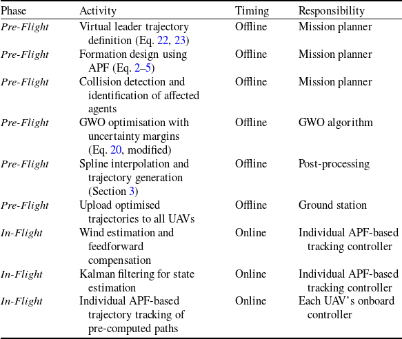
Once the nominal paths are determined, the collision status of each UAV with respect to known obstacles can be systematically evaluated. The obstacle crossing mechanism is then activated locally for those agents whose virtual paths intersect the obstacle boundary. At this stage, the modified GWO algorithm optimises the deviation trajectory for the affected UAVs. The optimisation objective is twofold: (I) to minimise the path length and turning radius violations, thereby ensuring dynamic feasibility, and (II) to preserve the formation structure as much as possible by limiting the displacement of each optimised point from its virtual counterpart. Notably, the number of UAVs that collide with the obstacle is not restricted a priori; the algorithm handles scenarios ranging from a single affected agent to multiple UAVs on either side of the formation, as demonstrated in Figure 8(b). It is important to emphasise that the entire optimisation process is performed offline, prior to mission execution, based on pre-known obstacle information. The resulting optimal trajectories are then uploaded to the UAVs as reference paths to be followed during flight.
This hierarchical framework (kinematic leader guidance, APF-based formation maintenance and GWO-based offline path optimisation) is particularly advantageous in cooperative surveillance missions. In such applications, a V-shaped formation of fixed-wing UAVs can provide wide-area coverage with minimal sensor overlap while maintaining a cohesive track on a moving target. The collective deviation strategy ensures that the sensor footprint (e.g. electro-optical or synthetic aperture radar payloads) remains uniformly distributed even when the formation encounters no-fly zones, tall structures or restricted airspace that are known in advance from mission intelligence or digital maps. The explicit penalisation of inadequate turning radii in the cost function (Equation 20) is especially beneficial here, as it prevents abrupt manoeuvres that could degrade image quality, disrupt inter-UAV communication links or induce excessive actuator wear during prolonged loitering.
In SAR scenarios, mission planning often relies on pre-existing terrain data, satellite imagery and known hazard maps to design safe flight corridors before deployment. The proposed method is particularly suitable for such pre-mission planning phases, where the formation geometry and obstacle-crossing trajectories for all UAVs can be computed in advance, ensuring that the swarm enters the operational area with a fully validated and dynamically feasible flight plan. The adaptability to different apex angles (90°, 120° or 180°) allows mission planners to tailor the swarm geometry to the operational environment: a wider formation (e.g. 180°) maximises lateral coverage over open terrain, while a narrower formation (e.g. 90°) facilitates navigation through confined valleys, urban canyons or forested areas where obstacle distribution is known beforehand. The spline-based interpolation step ensures that the resulting trajectories are sufficiently smooth for autonomous flight controllers to track without exceeding the UAV’s bank-angle or load-factor limits, which is critical for long-duration SAR operations where actuator reliability and fuel efficiency are major concerns. Once the optimal paths are computed offline, they can be stored and executed by the UAVs throughout the mission, providing a reliable and repeatable solution for obstacle avoidance in static or slowly varying environments.
Furthermore, the scalability of the approach (demonstrated with up to 15 agents) suggests that it can be extended to larger swarms for distributed sensing tasks, such as environmental monitoring, border patrol or disaster assessment, where multiple UAVs must operate in proximity for extended periods. The virtual leader paradigm simplifies mission-level command, allowing a single operator to guide the entire formation while the low-level GWO-based optimiser handles local obstacle avoidance autonomously during the pre-flight planning stage. This separation of concerns reduces the cognitive load on human operators and enhances overall system robustness in cluttered environments with known static obstacles.
Finally, it is worth emphasising that the proposed method does not impose any intrinsic limitation on the number of UAVs that may simultaneously collide with an obstacle. Whether a single agent or multiple agents on both sides of the formation are affected, the optimisation process independently determines the optimal deviation for each colliding path while the formation control law continuously adjusts the remaining agents to preserve inter-agent distances. This flexibility renders the framework suitable for dense swarm operations in complex environments where multiple obstacle encounters are expected during mission planning.
6.0 Robustness analysis and practical implementation considerations
6.1 Limitations of idealised assumptions
The simulation framework presented in Sections 3 and 4 employs simplifying assumptions common in initial algorithmic validation [Reference Kahagh, Pazooki and Haghighi7, Reference Kahagh, Pazooki, Haghighi and Asadi19]: (I) perfect inter-agent communication with negligible latency; (II) ideal state estimation without sensor noise; and (III) wind-free environmental conditions. While these assumptions facilitate algorithmic development, practical deployment in operational missions such as cooperative surveillance and SAR (Section 5) requires careful consideration of their effects on the tracking of the pre-computed optimised trajectories.
As described in detail in Section 5, the proposed methodology follows a hierarchical two-stage design:
-
I. Stage 1 (Pre-Flight - Offline Design):
-
• The virtual leader’s kinematic trajectory is defined using Equations (22), (23).
-
• The formation control law based on APF in Equation (2) establishes and maintains the desired V-shaped formation geometry with prescribed inter-agent distances
$d_{ij}$
and apex angle
$\alpha$
. At this stage, the nominal paths for all agents are determined. -
• Collision status with known obstacles is evaluated for each agent’s nominal path, and the agents whose paths intersect the obstacle boundary are identified.
-
• The modified GWO algorithm optimises the obstacle-crossing trajectories for the affected agents by adjusting the deviation distances
$d_{i}$
in Equation (19). The cost function in Equation (20) simultaneously minimises path length, ensures appropriate turning radius and prevents obstacle collisions. Importantly, the number of agents that collide with the obstacle is unrestricted – the algorithm handles scenarios ranging from a single affected agent to multiple UAVs on either side of the formation, as demonstrated in Figure 8. -
• Spline interpolation generates smooth, dynamically feasible trajectories for all agents.
-
-
II. Stage 2 (In-Flight - Online Execution):
-
• The pre-computed optimal trajectories are uploaded to the UAVs as reference paths.
-
• Each agent employs an APF-based tracking controller individually to follow its assigned reference trajectory. This controller utilises the potential function framework to generate appropriate control inputs that guide each UAV along the pre-computed path while compensating for minor deviations.
-


Key Observation: As clearly stated in Section 5, the APF-based formation control law in Equation (2) is employed only during the pre-flight design phase to establish the nominal formation geometry and determine the desired positions of all agents relative to the virtual leader. During actual flight, the UAVs execute the pre-computed trajectories using individual APF-based tracking controllers, not a formation-level APF controller that actively adjusts the formation in response to environmental disturbances. Consequently, the kinematic model in Equation (1) describes the intended motion during the design phase, but the actual motion during flight is subject to tracking errors arising from environmental disturbances. The formation geometry and inter-agent distances
 $d_{ij}$
that were established during the offline design phase are expected to be maintained only if each UAV accurately tracks its assigned reference trajectory using its individual APF-based tracking controller.
6.1.1 Wind disturbances
During flight execution, wind causes the UAV to deviate from its pre-computed reference trajectory. The actual kinematic relationship differs from the design model:
 \begin{equation}{\dot{p}}_{i}^{\textit{actual}}={\dot{p}}_{i}^{\textit{reference}}+W(p_{i},t)\end{equation}
where
 ${\dot{p}}_{i}^{\textit{reference}}$
is the desired velocity from the pre-computed trajectory, and
 $W(p_{i},t)$
denotes the wind velocity vector. This mismatch introduces:
-
I. Tracking Errors: Wind causes the UAV to deviate from its pre-computed reference trajectory, potentially violating the desired inter-agent distances
$d_{ij}$
that were established during the offline formation design using the APF method. While the individual APF-based tracking controller attempts to keep each UAV on its reference path, its performance may be degraded under strong wind conditions. -
II. Impact on Obstacle Avoidance: The optimised obstacle-crossing trajectory was computed assuming no wind. Wind-induced drift may cause the UAV to approach the obstacle boundary more closely than intended, potentially compromising the safety margin
$S.M$
defined in the cost function. The minimum turning radius
$R_{m}={v}_{min}^{2}/(g\mathit{\tan } (\phi _{max}))$
may also become infeasible if wind assists or opposes the turn.


6.1.2 Sensor noise
During trajectory tracking, the UAV relies on onboard sensors for state estimation. The individual APF-based tracking controller uses these measurements as feedback. Table 6 presents the noise characteristics that may influence the trajectory tracking performance.
Sensor noise sources and their effects on reference trajectory following

Table 6. Long description
A table with three columns and four rows, including a header row. The columns are labeled Noise source, Typical magnitude, and Effect on trajectory tracking. The rows list different noise sources and their characteristics. Row 1: GPS position error, 1-5 m (standard), 0.1-1 m (RTK), Errors in position feedback for the APF tracking controller. Row 2: IMU velocity drift, 0.1-0.5 m/s, Accumulated position errors. Row 3: Airspeed measurement error, 0.5-2 m/s, Errors in wind estimation.
6.2 Proposed adaptations for real-world implementation
Since the GWO optimisation is performed offline (as described in Section 5) and the optimised trajectories are provided to the UAVs as reference paths, the proposed adaptations focus on two complementary aspects: (I) enhancing the offline optimisation to account for expected uncertainties, and (II) improving the online tracking through individual APF-based feedback control to ensure accurate execution of the pre-computed trajectories.
6.2.1 Pre-flight phase enhancements (offline GWO optimisation)
Since the GWO optimisation determines the deviation distances
 $d_{i}$
Equation (19) based on the virtual path, the following enhancements can be incorporated into the cost function and constraints without altering the fundamental optimisation structure:
-
I. Uncertainty-Aware Cost Function: The GWO optimisation in Equation (20) can incorporate uncertainty margins directly:
(25)where
\begin{equation}J_{\textit{robust}}=\omega _{l}.\sum\limits_{n=1}^{N_{p}}\left(\Delta L_{n}\right)+\omega _{tr}.N_{tr}+\omega _{o}.N_{o}+\omega _{unc}.\sum\limits_{n=1}^{N_{p}}\left({\sigma }_{n}^{2}\right)\end{equation}
${\sigma }_{n}^{2}$
is the expected position variance at point
$n$
(estimated from sensor specifications), and
$\omega _{unc}$
penalises trajectories that approach obstacles within the measurement uncertainty margin. This ensures that the pre-computed trajectories maintain safe clearance considering sensor limitations that will affect the individual APF-based tracking controllers during flight.


-
II. Adaptive Safety Margin: The safety margin
$S.M$
in the obstacle boundary constraint can be calibrated based on expected tracking uncertainty:(26)where
\begin{equation}S.M_{eff}=S.M_{\textit{nominal}}+\sigma _{\textit{position}}\end{equation}
$\sigma _{\textit{position}}$
is the
$3\sigma$
position uncertainty. A larger safety margin ensures the optimised trajectory remains collision-free despite tracking errors during flight, providing the individual APF-based tracking controllers with sufficient clearance to operate safely.


-
I. Wind-Robust Turning Radius Constraint: Since wind during flight may degrade turning performance, the minimum turning radius constraint can be augmented:
(27)where
\begin{equation}R_{m,eff}=R_{m}+\gamma _{\omega }.{||\hat{W}_{\textit{expected}}|| \over v_{min}}.R_{m}\end{equation}
$\hat{W}_{\textit{expected}}$
is the anticipated wind speed from meteorological data, and
$\gamma _{\omega }$
accounts for wind-induced degradation.


6.2.2 In-flight phase enhancements (online tracking control)
Following the offline GWO optimisation and spline interpolation (Section 3), the optimised trajectories are uploaded to the UAVs as reference paths. During flight, each UAV employs an individual APF-based tracking controller to follow its reference trajectory. The following enhancements ensure accurate tracking:
-
I. Wind Estimation and Feedforward Compensation: Since wind is the primary source of tracking errors, a real-time wind estimation filter can be integrated into each UAV’s tracking control loop:
(28)where
\begin{equation}\hat{W}(t)=\dot{\hat{p}}_{i}(t)-v_{\textit{airspeed}}(t)\end{equation}
$\dot{\hat{p}}_{i}(t)$
is the estimated velocity from GPS, and
$v_{\textit{airspeed}}(t)$
is the measured airspeed. The estimated wind is used to generate feedforward compensation for the individual APF-based tracking controller:(29)where
\begin{equation}{u}_{i}^{comp}={u}_{i}^{APF}-\hat{W}(t)\end{equation}
${u}_{i}^{APF}$
is the control signal generated by the individual APF-based tracking controller. This reduces steady-state tracking errors without requiring gain increases that could excite unmodeled dynamics.


-
II. Kalman Filter for State Estimation: Implement a discrete-time Kalman filter for each agent:
(30)where
\begin{equation}\hat{p}_{i}{\left(k|k\right)}=\hat{p}_{i}{\left(k|k-1\right)}+K_{k}{[z_{i}(k)-H\hat{p}_{i}(k|k-1)]}\end{equation}
$z_{i}(k)$
is the noisy measurement vector (GPS/IMU), and
$K_{k}$
is the optimal Kalman gain. This provides smoothed position estimates to the individual APF-based tracking controller, reducing the effects of sensor noise on tracking performance.


-
III. Adaptive Formation Expansion: If the estimated tracking uncertainty exceeds a threshold during flight, the formation can be dynamically expanded by increasing the inter-agent distance
$d_{ij}$
:(31)
\begin{equation} {d}_{ij}^{\textit{adapt}}={d}_{ij}^{\textit{nominal}}+\delta _{\textit{uncertainty}}\end{equation}


This maintains safety without requiring online GWO re-optimisation, which is computationally infeasible for onboard processors. The individual APF-based tracking controllers will then operate with larger safe margins. Consistent with the two-stage design philosophy described in Section 5, the proposed implementation maintains the following separation (Table 7):
Summary of implementation architecture

Table 7. Long description
A table summarizing the implementation architecture for UAV missions. The table has four columns: Phase, Activity, Timing, and Responsibility. It contains ten rows detailing various activities and their respective timings and responsibilities. The phases are divided into Pre-Flight and In-Flight. Pre-Flight activities include virtual leader trajectory definition, formation design using APF, collision detection, GWO optimization, spline interpolation, and uploading optimized trajectories. In-Flight activities include wind estimation, Kalman filtering, and trajectory tracking. Each activity is assigned a specific responsibility such as Mission planner, GWO algorithm, Post-processing, Ground station, Individual APF-based tracking controller, and Each UAV’s onboard controller.
The proposed adaptations preserve the core contribution of this work (the modified GWO algorithm for offline optimisation of obstacle avoidance trajectories) while adding the robustness necessary for practical implementation. During flight, each UAV employs an individual APF-based tracking controller to follow its pre-computed reference trajectory. The in-flight enhancements (wind estimation with feedforward compensation, Kalman filtering and adaptive formation expansion) serve only to ensure accurate tracking of the pre-computed paths, not to modify the optimised trajectories online. The APF-based tracking controller operates independently for each agent, generating appropriate control inputs based on the difference between the agent’s current position and its desired position on the reference trajectory.
This separation of offline optimisation and online tracking control offers several practical advantages:
-
• The computationally intensive GWO optimisation does not burden onboard processors.
-
• Mission planners can validate trajectories before deployment.
-
• Contingency paths can be pre-computed for multiple obstacle configurations.
-
• The formation can adapt to uncertainty through expansion rather than replanning.
-
• The number of affected agents does not affect the computational complexity of the individual tracking controllers.
-
• Each UAV’s APF-based tracking controller operates independently, providing inherent scalability.
7.0 Conclusion
The results show that the defined cost function, constraints and, most importantly, the method for defining the decision variables in the GWO algorithm, perform well in solving the optimisation problem and provide a suitable path for passing the obstacle. By considering the distance of each point from the virtual path to the corresponding point on the real path as the decision variable, only one distance variable is used instead of the two components x and y. This approach reduces the complexity and dimension of the problem.
A constraint was incorporated into the optimisation problem to move path points that fall inside the obstacle to a safe position. This quickly generates a collision-free path and prevents the obstacle from approaching along other paths.
Furthermore, using appropriate values for the initial population of wolves to create a reasonably good path, or creating a suitable initial path for one of the wolves, can reduce the search space and push the algorithm’s responses towards greater convergence. Given that the number of decision variables is in the range of 20, 30, 45, etc., it is challenging to find a path for this number of points that has a suitable turning radius and sufficient curvature. This approach significantly reduces the number of broken paths and eliminates the need for many iterations in the search phase of the algorithm. Therefore, a function for the parameter
 $a$
was proposed that has a greater tendency toward local search (exploitation). To ensure a path with a suitable turning radius, a term was included in the cost function that applies a penalty to points with an inappropriate turning radius, thereby creating a dynamically suitable path for the UAV. Additionally, a smooth path was created by fitting a spline to the points, and interpolation was performed to increase the number of path points.
The practical relevance of the proposed framework is further underscored by its applicability to cooperative surveillance and SAR missions. In such scenarios, the hierarchical control architecture (combining kinematic leader guidance, APF-based formation maintenance and GWO-based path optimisation) provides a systematic and reliable solution for pre-mission trajectory planning in environments with known static obstacles. The offline nature of the optimisation process ensures that all trajectories are fully validated for dynamic feasibility and formation integrity before deployment, thereby minimising in-flight computational burden and enhancing mission safety. Moreover, the scalability of the algorithm, which imposes no intrinsic restriction on the number of UAVs simultaneously colliding with an obstacle, makes it particularly suitable for dense swarm operations in complex terrains.
While the current simulations assume idealised conditions, we have identified practical challenges (wind disturbances, sensor noise, and communication latency) that affect the tracking of pre-computed optimised trajectories during flight. Consistent with the two-stage design philosophy, we have proposed adaptations that preserve the offline optimisation structure while enhancing in-flight tracking robustness. These include: (I) pre-flight enhancements to the GWO optimisation (uncertainty-aware cost functions, adaptive safety margins, wind-robust turning radius constraints); and (II) in-flight enhancements for accurate trajectory tracking using individual APF-based tracking controllers (wind estimation with feedforward compensation, Kalman filtering and adaptive formation expansion).
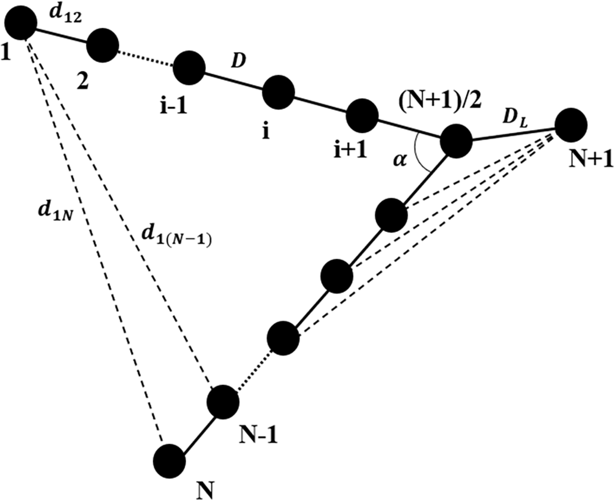


 a
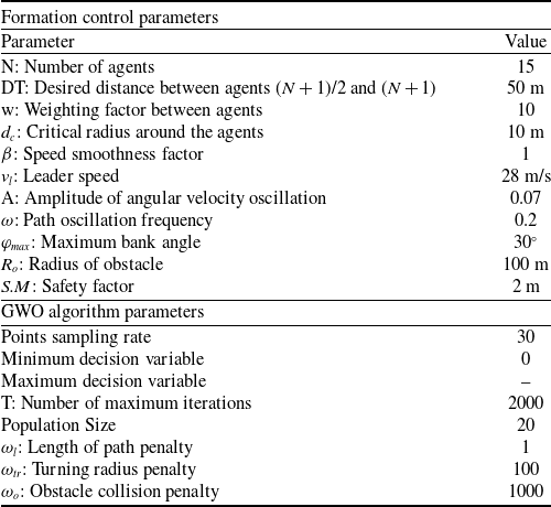


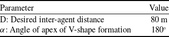
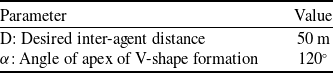
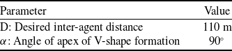

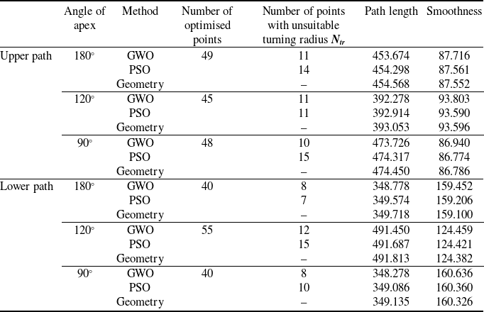

 No
 Ntr
 ωo
 ωtr