Thermal effect in shock-induced gas filtration through porous media

Jiarui Li; Jun Chen; Baolin Tian; Meizhen Xiang; Kun Xue

doi:10.1017/jfm.2024.699

Thermal effect in shock-induced gas filtration through porous media

Published online by Cambridge University Press: 22 November 2024

and

Jiarui Li: Affiliation:
National Key Laboratory of Computational Physics, Institute of Applied Physics and Computational Mathematics, Beijing 100088, PR ChinaState Key Laboratory of Explosive Science and Technology, Beijing Institute of Technology, Beijing 100081, PR China
Jun Chen: Affiliation:
National Key Laboratory of Computational Physics, Institute of Applied Physics and Computational Mathematics, Beijing 100088, PR China
Baolin Tian: Affiliation:
School of Aeronautic Science and Engineering, Beihang University, Beijing 100191, PR China
Meizhen Xiang: Affiliation:
National Key Laboratory of Computational Physics, Institute of Applied Physics and Computational Mathematics, Beijing 100088, PR China
Kun Xue*: Affiliation:
State Key Laboratory of Explosive Science and Technology, Beijing Institute of Technology, Beijing 100081, PR China
*: †Email address for correspondence: xuekun@bit.edu.cn

Article contents

Abstract
Introduction
Methods
Numerical set-up
Results and analysis
Discussion
Conclusion
Glossary
Declaration of interests
References

Rights & Permissions

Abstract

The gas dynamics of shock-induced gas filtration through densely packed granular columns with vastly varying shock intensity and the structural parameters are numerically investigated using a coupled Eulerian–Lagrangian approach. The results shed fundamental light on the thermal effects of the shock-induced gas filtration manifested by a distinctive self-heating hot gas layer traversing the medium. The characteristics of the thermal effects in terms of the thermal intensity and uniformity are found to vary with the shock Mach number, Ms, and the filtration coefficient of the granular media, Π. As the incident shock transitions from weak to strong, and (or) the filtration coefficient increases from O(10−5) to O(104), the heating mechanisms transition between three distinct heating modes. A phase diagram of heating modes is established on the parameter space (Ms, Π), which enables us to predict the characteristics of the thermal effect in different shock-induced gas filtrations. The thermal effects markedly accelerate the pressure diffusion due to the additional heat influx when the time scale of the former is smaller than or comparable to the latter. Based on the contour map displaying the coupling degree of the thermal effects and the pressure diffusion, we identify a decoupling criterion whereby the isothermal assumption holds if only the pressure diffusion is concerned. The thermal effects may well bring about considerable thermal shocks which pose a great threat to the integrity of the solid skeleton and further reduce the overall shock resistance performance of the porous media.

JFM classification

Multiphase and Particle-laden Flows: Particle/fluid flow Compressible Flows: Shock waves Compressible Flows: Gas dynamics

Information

Type: JFM Papers
Information: Journal of Fluid Mechanics , Volume 999 , 25 November 2024, A91
DOI: https://doi.org/10.1017/jfm.2024.699 [Opens in a new window]
Copyright: © The Author(s), 2024. Published by Cambridge University Press

1. Introduction

Flow in porous media has numerous applications in environmental protection, including groundwater mitigation (Bear & Alexander Reference Bear and Alexander2010; Pathak & Singh Reference Pathak and Singh2015; Eriksen et al. Reference Eriksen, Toussaint, Turquet, Måløy and Flekkøy2018; Xue et al. Reference Xue, Li, Nan and Wu2019; Flekkøy, Sandnes & Måløy Reference Flekkøy, Sandnes and Måløy2023), underground contaminant transport (Hayek Reference Hayek2017; Shen et al. Reference Shen, Huang, Illman, Su and Miao2023), carbon capture and geological sequestration (Abidoye, Khudaida & Das Reference Abidoye, Khudaida and Das2015; De Paoli, Zonta & Soldati Reference De Paoli, Zonta and Soldati2016). In contrast to the aforementioned applications characterized by relatively low speed, the primary focus of this paper is on the phenomenon of shock-induced interstitial flow. Blast waves generated through the detonation of high explosives pose a serious hazard to individuals and structures in close proximity. Therefore, the mitigation of blast waves is a crucial practical concern (Britan et al. Reference Britan, Ben-Dor, Igra and Shapiro2001; Ji, Li & Chen Reference Ji, Li and Chen2012; Frost Reference Frost2018; Gubin Reference Gubin2018; Pontalier et al. Reference Pontalier, Loiseau, Goroshin and Frost2018). Numerous porous media, such as granular material or aqueous foam, have been utilized as protective screens to mitigate blast energy (Skews Reference Skews2001; Smith Reference Smith2010; Petel et al. Reference Petel, Jetté, Goroshin, Frost and Ouellet2011; Britan et al. Reference Britan, Shapiro, Liverts, Ben-Dor, Chinnayya and Hadjadj2013; Del Prete et al. Reference Del Prete, Chinnayya, Domergue, Hadjadj and Haas2013; Vivek & Sitharam Reference Vivek and Sitharam2019). The head-on collision of normal shock waves with porous materials has been extensively studied as a prototype to investigate blast mitigation mechanisms, thereby garnering considerable attention in past decades (Gvozdeva, Faresov & Fokeev Reference Gvozdeva, Faresov and Fokeev1985; Henderson et al. Reference Henderson, Virgona, Di and Gvozdeva1990; Skews Reference Skews1991; Ben-Dor et al. Reference Ben-Dor, Mazor, Igra, Sorek and Onodera1994).

The interactions of shock waves with porous media consist of two fundamental processes (Ben-Dor et al. Reference Ben-Dor, Britan, Elperin, Igra and Jiang1997; Skews Reference Skews2001; Yin et al. Reference Yin, Ding, Luo and Yu2019; Han, Xue & Bai Reference Han, Xue and Bai2021; Li et al. Reference Li, Zeng and Xue2023), as shown in figure 1. One is the intricate interaction between the transmitted wave and the skeleton of porous media. As particles constituting the porous medium move under the impact of shock waves, the contact among the particles increases, leading to a more densely packed medium. This phenomenon is referred to as compaction. During compaction, the solid stress propagates through contacts between particles, forming a compaction wave within the skeleton. The local particle volume fraction increases as the compaction front passes. The other involves gas penetration driven by a significant pressure difference between the reflected shock upstream and the ambient air downstream. This phenomenon, referred to as filtration in the literature, leads to an increase in the gas pressure within the pores, which is abbreviated as pore pressure (Britan et al. Reference Britan, Ben-Dor, Elperin, Igra and Jiang1997). Since the transmitted wave rapidly decays during propagation, particularly in granular materials with low porosity, the compaction wave and gas filtration in long porous media with low to moderate porosities are of major concern (Rogue et al. Reference Rogue, Rodriguez, Haas and Saurel1998; Sadot et al. Reference Sadot, Ram, Ben-Dor, Levy, Golan, Ran and Aizik2013). For flexible aqueous foams (polyurethane or polyethylene) or loosely packed granular materials, an interaction between the compaction wave and gas filtration is observed (Skews et al. Reference Skews, Atkins, Seitz and Takayama1992; Levy et al. Reference Levy, Ben-Dor, Skews and Sorek1993). Our previous study demonstrated that the presence of a fast-advancing compaction front would produce a deflection in the spatial distribution of the pore pressure due to the reduction in porosity (Li et al. Reference Li, Zeng and Xue2023). The drag force exerted between the two phases involved in gas filtration would subsequently alter the compaction process (Ben-Dor et al. Reference Ben-Dor, Britan, Elperin, Igra and Jiang1997; Xue et al. Reference Xue, Miu, Li, Bai and Tian2023). However, the compaction is minimal for rigid or densely packed granular materials, where the solid skeleton can be assumed to be motionless (Rogg et al. Reference Rogg, Hermann and Adomeit1985; Ram & Sadot Reference Ram and Sadot2015). In this scenario, the shock–particle interaction is solely determined by gas filtration through granular media.

Figure 1.

Schematic diagrams of the two fundamental processes involved in the interaction of shock waves with porous media. (a) Compaction of the solid phase. (b) Gas filtration within the pores.

Many experimental and numerical studies have been published on the topic of shock-induced gas filtration through rigid porous media. The experiments are typically carried out in vertical shock tubes, with the pressure history being measured by transducers mounted along the sidewalls and end wall. The objectives of these studies were to investigate the impact of shock strength, porosity, particle size and propagation distance on gas pressure. Due to the limited availability of the pressure transducers, a continuous pressure evolution law is difficult to establish. As a result, quantitative conclusions are derived by fitting limited pressure profiles. Experiments provide qualitative trends at the macroscale, but they do not capture microscale information such as local flow velocity or porosity changes. Therefore, numerical simulations provide a promising approach to investigate gas filtration and determine the underlying mechanism.

Notable progress was made by Morrison in his endeavour to mathematically describe the gas filtration induced by a nuclear underground explosion (Morrison Reference Morrison1972). In Morrison's approach, the pressure gradient in the filtration flow, denoted as $\partial P/\partial x$, depends on the interstitial gas velocity $\tilde{\boldsymbol{V}}$ in a generalized form that is commonly known as the Forchheimer resistance law (Lage Reference Lage, Ingham and Pop1998):

(1.1)

\begin{equation}\frac{{\partial P}}{{\partial x}} ={-} a\mu \tilde{\boldsymbol{V}} - b\rho \tilde{\boldsymbol{V}}|{\tilde{\boldsymbol{V}}} |.\end{equation}

The first term on the right-hand side of (1.1) is called the Darcy term $- a\mu \tilde{\boldsymbol{V}}$, and it accounts for viscous losses where μ is the gas viscosity. The Darcy coefficient, a, is related to the permeability, k, and porosity, ε, by the equation a = ε/k. The second term is the Forchheimer term $- b\rho \tilde{\boldsymbol{V}}|{\tilde{\boldsymbol{V}}} |$, where ρ is the gas density and b is the Forchheimer coefficient, and this term models the inertial loss. A non-dimensional parameter, the effective Reynolds number, Re_f, has been introduced to quantify the relative significance of these two terms. Gas filtration with Re_f < 1 and Re_f → ∞, where the Forchheimer/Darcy term becomes negligible, was specified as Darcy-flow and Forchheimer-flow domains, respectively. Both Darcy flow and Forchheimer flow exhibit self-similar solutions for the pore pressure field, albeit with different scaling laws. Following Morrison's approach, Britan et al. introduced the thresholds of Re_f for classifying various flow regimes (including Darcy flow, Forchheimer flow and mixed flow between) based on the Mach number of the incident shock (Britan, Shapiro & Ben-Dor Reference Britan, Shapiro and Ben-Dor2007). In addition, a hybrid method was developed to determine the values of the Darcy and Forchheimer coefficients (a and b) via controlled shock tube experiments and then enabled reconstruction of the pressure profiles at different locations within a granular sample (Britan et al. Reference Britan, Ben-Dor, Igra and Shapiro2006).

The self-similar solution obtained from the Morrison approach requires steady boundary conditions, specifically maintaining the upstream pressure after the shock wave reflects off the front surface of the porous column, P ₅, unchanged. The aforementioned requirements are barely met in shock tube experiments due to multiple reflections and complex wave interactions that occur within the porous column and in field tests. Hence, the Morrison method was modified by incorporating an unsteady upstream pressure as a boundary condition, based on the experimental data (Britan et al. Reference Britan, Ben-Dor, Igra and Shapiro2006). The Morrison approach, which is relatively simplified, showed performance comparable to that of the full solution based on the complete system of conservation equations in accurately reproducing the pressure histories in the shock-impacted granular columns (Britan et al. Reference Britan, Ben-Dor, Igra and Shapiro2006).

Although Morrison's model and its variants have the capability to simulate the transient pressure diffusion of gas filtration through granular columns, they do not incorporate the thermodynamic evolution of interstitial flow. The flow temperature was considered to be equivalent to that of the solid phase, with both maintaining ambient temperature. This isothermal assumption becomes problematic as the intensity of the shock increases. Since the temperature of the upstream reflected shock, T ₅, is dependent on the shock intensity, the gases upstream experience significant heating. In addition to the temperature difference between the upstream surface and that inside porous media, the compressible nature of the gas infiltration enables the exchange of kinetic energy and internal energy, indicating that the kinematic and thermodynamic parameters are interdependent during gas filtration. Evidently, the isothermal assumption is invalid in scenarios involving strong shock waves. Therefore, the applicability of the Morrison approach needs to be revisited. Although some full numerical methods considering the energy conversion of the flow have been employed in gas infiltration research in recent years, the majority of these studies focus on the relationship between the pressure evolution and initial parameters such as shock intensity, porosity and particle size. The fundamental question of the extent to which the thermodynamic evolution of gases influences the flow parameters of the shock-induced gas filtration remains unresolved.

The primary objective of this study is to gain insight into the thermal effect in shock-induced gas filtration and to determine the correlation between the thermodynamic and dynamic parameters. Full solutions consisting of the mass, momentum and energy conservation equations are viable options for accessing the potential thermal effect. Some of the full solutions treat both the gas and solid phases as a continuum, suggesting that the average flow parameters are minimally affected by local heterogeneity (Baer & Nunziato Reference Baer and Nunziato1986; Petitpas et al. Reference Petitpas, Franquet, Saurel and Le Metayer2007; Saurel et al. Reference Saurel, Chinnayya and Carmouze2017). Moreover, the gas flow velocity is assumed to be low such that the unsteady effects are minimal (Crowe et al. Reference Crowe, Schwarzkopf, Sommerfeld and Tsuji2012). Evidently, these assumptions cannot universally hold in granular media composed of randomly packed particles with vastly varying sizes. To overcome these constraints, the discrete-element method (Patankar & Joseph Reference Patankar and Joseph2001; O'Rourke & Snider Reference O'Rourke and Snider2010; Snider et al. Reference Snider, Clark and O'Rourke2011; Balachandar Reference Balachandar2012; Alobaid & Epple Reference Alobaid and Epple2013; Guo et al. Reference Guo, Wassgren, Hancock, Ketterhagen and Curtis2015; Mo et al. Reference Mo, Lien, Zhang and Cronin2019; Jiang et al. Reference Jiang, Guo, Yu, Hua, Lin, Wassgren and Curtis2021; Qiao et al. Reference Qiao, Liu and Ji2022) is employed to generate a solid skeleton with particle-scale randomness. By coupling compressible computational fluid mechanics and the discrete-element method, referred to as CMP-PIC in our previous publications (Tian et al. Reference Tian, Zeng, Meng, Chen, Guo and Xue2020), we can consider the flow variation at the particle scale and conduct parametric studies on the variables relevant to the granular assembly.

In the following, brief accounts of CMP-PIC and the Morrison approach are presented in § 2. The numerical set-up is provided in § 3. The dynamics of the flow parameters during shock-induced gas filtration is described in § 4.1. The thermal effects characterized by the spatiotemporal evolution of the thermodynamic parameters are analysed in § 4.2. The mechanisms governing thermal effects and their influences on the flow parameters are discussed in § 4.3. The different domains of the thermal effects are defined in § 4.4, and the phase diagram is established in the parameter space comprising two essential non-dimensional parameters. The implications of thermal effects on granular media as protective shields, as well as the validity of the isothermal assumption for shock-induced gas infiltration, are discussed in § 5. A brief summary is provided in § 6.

2. Methods

2.1. The CMP-PIC approach

Numerical simulations were performed based on CMP-PIC, a coarse-grained Euler–Lagrange approach suitable for gas–particle flows in laboratory-scale systems (Sundaresan et al. Reference Sundaresan, Ozel and Kolehmainen2018; Koneru et al. Reference Koneru, Rollin, Durant, Ouellet and Balachandar2020). The CMP-PIC approach tracks and accounts for contact interactions between parcels. Each parcel consists of multiple individual particles with the same physical and kinetic properties. The number of real particles that constitutes a computational parcel is quantified using a scaling factor called the super particle loading, α ², whose value is set based on the volume/mass fraction of the particles and computational memory available. For particle–gas systems, the reported α ² in previous literature ranges from O(10¹) to O(10³) (Osnes et al. Reference Osnes, Vartdal and Pettersson Reif2017; Koneru et al. Reference Koneru, Rollin, Durant, Ouellet and Balachandar2020; Xue et al. Reference Xue, Shi, Zeng, Tian, Han, Li, Liu, Meng, Guo and Bai2020). In the present work, α ² is of O(10¹).

For the gas phase, the volume-averaged governing equations (2.1)–(2.3) constructed in the Eulerian frame are based on a five-equation transport model, i.e. a simplified form of the Baer–Nunziato model (Baer & Nunziato Reference Baer and Nunziato1986); this model has been modified to account for compressible multiphase flows ranging from dilute to dense gas–particle flows (Carmouze et al. Reference Carmouze, Saurel, Chiapolino and Lapebie2020; Chiapolino & Saurel Reference Chiapolino and Saurel2020).

(2.1)

\begin{gather}\frac{{\partial (\varepsilon {\rho _f})}}{{\partial t}} + \boldsymbol{\nabla }\boldsymbol{\cdot }(\varepsilon {\rho _f}{\boldsymbol{u}_f}) = 0,\end{gather}

(2.2)

\begin{gather}\frac{{\partial (\varepsilon {\rho _f}{\boldsymbol{u}_f})}}{{\partial t}} + \boldsymbol{\nabla }\boldsymbol{\cdot }(\varepsilon {\rho _f}{\boldsymbol{u}_f}{\boldsymbol{u}_f}) + \boldsymbol{\nabla }(\varepsilon {P_f}) = {P_f}\boldsymbol{\nabla }\varepsilon + \sum_i {[{\phi _{p,i}}{\rho _{p,i}}{D_{p,i}}({\boldsymbol{u}_{p,i}} - {{\bar{\boldsymbol{u}}}_f})]} ,\end{gather}

(2.3)

\begin{gather}\frac{{\partial (\varepsilon {\rho _f}{E_f})}}{{\partial t}} + \boldsymbol{\nabla }\boldsymbol{\cdot }(\varepsilon {\rho _f}{E_f}{\boldsymbol{u}_f} + \varepsilon {P_f}{\boldsymbol{u}_f}) = {P_f}\boldsymbol{\nabla }\varepsilon \boldsymbol{\cdot }{\bar{\boldsymbol{u}}_p} + \sum_i {[{\phi _{p,i}}{\rho _{p,i}}{D_{p,i}}({\boldsymbol{u}_{p,i}} - {{\bar{\boldsymbol{u}}}_f})\boldsymbol{\cdot }{\boldsymbol{u}_{p,i}}].}\end{gather}

The volume fraction of gas phase, i.e. porosity, is expressed by ε. The volume fraction of particle phase is expressed by ϕ_p, while ε + ϕ_p = 1 in the same fluid grid. The velocity, density, pressure and total energy of the gas are represented by u_f, ρ_f, P_f and E_f, respectively. Here E_f = e_f + 0.5u_fu_f, where e_f is the specific internal energy. Terms ϕ_p _.i, ρ_p _.i, D_p _,i and u_p _,i are local volume fraction, density, drag force coefficient and velocity of parcel i. Parameter ū_f represents the average fluid velocity at the location of particle i and ū_p represents the average velocity of particles within a fluid cell. Notably, the first term on the right-hand side of (2.2), P_f ∇ε, is the nozzling term that becomes significant wherever the porosity gradient is non-trivial.

We employ the Di Felice model combined with Ergun's equation to calculate D_p, which is essentially a nonlinear drag force model (Di Felice Reference Di Felice1994). The Di Felice model combined with Ergun's equation (Ergun Reference Ergun1952) considers the effects of both the particle Reynolds number, Re_p, and the porosity, ε, and has been widely used in particle-laden multiphase flows (Kafui, Thornton & Adams Reference Kafui, Thornton and Adams2002; Feng et al. Reference Feng, Xu, Zhang, Yu and Zulli2004). Parameter D_p is a function of Re_p and ε:

(2.4)

\begin{gather}{D_{p,i}} = \frac{3}{{8sg}}{C_d}\frac{{|{{{\bar{\boldsymbol{u}}}_f} - {\boldsymbol{u}_{p,i}}} |}}{{{r_p}}},\end{gather}

(2.5)

\begin{gather}{C_d} = \frac{{24}}{{R{e_p}}}\left\{ {\begin{array}{@{}l@{\quad}c@{}} {8.33\dfrac{{1 - \varepsilon }}{\varepsilon } + 0.0972R{e_p}}&{\textrm{if}\;\varepsilon < 0.8,}\\ {{f_{base}} \cdot {\varepsilon^{ - \zeta }}}&{\textrm{if}\;\varepsilon \ge 0.8,} \end{array}} \right.\end{gather}

(2.6)

\begin{gather}{f_{base}} = \left\{ {\begin{array}{@{}l@{\quad}c@{}} {1 + 0.167Re_p^{0.687}}&{\textrm{if}\;R{e_p} < 1000,}\\ {0.0183R{e_p}}&{\textrm{if}\;R{e_p} \ge 1000,} \end{array}} \right.\end{gather}

(2.7)

\begin{gather}\zeta = 3.7 - 0.65\,\textrm{exp}[ - {\textstyle{1 \over 2}}{(1.5 - {\log _{10}}R{e_p})^2}],\end{gather}

where C_d is the dimensionless coefficient of the drag force, sg is the specific weight of individual particles, sg = ρ_p/ρ_f, and r_p is the particle radius. For dense particle flows (ε < 0.8), (2.4) reduces to the original Ergun equation. Otherwise, C_d takes the form of the Stokes law multiplied by a correction coefficient which varies with Re_p, as indicated by (2.6) and (2.7).

The particle phase is represented by discrete parcels whose motion is governed by Newton's second law ((2.8) and (2.9)):

(2.8)

\begin{gather}\frac{{\textrm{d}{\boldsymbol{u}_{p,i}}}}{{\textrm{d}t}} = {D_{p,i}}({\bar{\boldsymbol{u}}_f} - {\boldsymbol{u}_{p,i}}) - \frac{1}{{{\rho _p}}}\boldsymbol{\nabla }\langle {P_f}\rangle + \frac{1}{{{m_p}}}\sum_j {{\boldsymbol{F}_{C,ij}}} ,\end{gather}

(2.9)

\begin{gather}\frac{{\textrm{d}\kern0.7pt{\boldsymbol{x}_{p,i}}}}{{\textrm{d}t}} = {\boldsymbol{u}_{p,i}},\end{gather}

where x_p _,i and m_p _,i denote the displacement and mass of parcel i, respectively, and F_C _,ij represents the collision force between parcels i and j.

A four-way coupling strategy (Ukai et al. Reference Ukai, Balakrishnan and Menon2010) was adopted to account for the momentum and energy transfer between the gases and particles. Specifically, the drag force and the associated work from particles were incorporated into the momentum (2.2) and energy (2.3) equations of the gas phase as the source terms. The parcels are driven by the pressure gradient force, drag force and collision force between themselves (equation (2.8)). A soft sphere model, represented by a coupling spring and dashpot, was employed to model the collision force between the parcels (Apte, Mahesh & Lundgren Reference Apte, Mahesh and Lundgren2003). Hence, F_C,ij consists of a repulsive force and a damping force, as follows:

(2.10)

\begin{equation}{\boldsymbol{F}_{C,ij}} = {k_{n,p}}{\boldsymbol{\delta }_n} - {\gamma _{n,p}}{\boldsymbol{u}_{n,ij}},\end{equation}

where k_n _,p and γ_n _,p are the stiffness and damping coefficients of the parcels, respectively, and δ_n and u_n _,ij are the overlap and normal velocity difference between parcels in contact, respectively. Here γ_n _,p is a function of the parcel restitution coefficient e_p (Crowe et al. Reference Crowe, Schwarzkopf, Sommerfeld and Tsuji2012) and defined as follows:

(2.11)

\begin{equation}{\gamma _{n,p}} ={-} \frac{{2\,\textrm{ln}\,{e_p}}}{{\sqrt {{{\rm \pi} ^2} + \textrm{ln}\,{e_p}} }}\sqrt {{m_p}{k_{n,p}}} .\end{equation}

To solve the equations governing the gases, the weighted essentially non-oscillatory (Liu et al. Reference Liu, Osher and Chan1994) scheme was used to reconstruct the primary flow variables. A Riemann solver proposed by Harten, Lax and van Leer (Toro Reference Toro2013) was used to obtain the intercell fluxes. The third-order Runge–Kutta method was applied for the time integration. The equations describing the parcel velocity and position were discretized by the velocity-Verlet algorithm (Kruggel-Emden et al. Reference Kruggel-Emden, Sturm, Wirtz and Scherer2008). Bilinear/trilinear interpolation functions were adopted to calculate the particle volume fraction and source terms on the Eulerian grids, as well as the fluid variables on the Lagrangian parcels. Numerical details with regard to CMP-PIC can be found in our previous studies (Meng et al. Reference Meng, Zeng, Tian, Li, He and Guo2019; Tian et al. Reference Tian, Zeng, Meng, Chen, Guo and Xue2020; Xue et al. Reference Xue, Shi, Zeng, Tian, Han, Li, Liu, Meng, Guo and Bai2020; Li et al. Reference Li, Xue, Zeng, Tian and Guo2021).

The present CMP-PIC framework has been validated against Rogue's experiments involving shock waves propagating through particle curtains (Tian et al. Reference Tian, Zeng, Meng, Chen, Guo and Xue2020), shock tube experiments wherein particle columns are impinged head-on by incident shocks (Tian et al. Reference Tian, Zeng, Meng, Chen, Guo and Xue2020) and shock dispersion of particle rings (Xue et al. Reference Xue, Shi, Zeng, Tian, Han, Li, Liu, Meng, Guo and Bai2020). Specifically, CMP-PIC reproduces the pore pressure histories at the cross-sections along the length of the granular columns with different distances from the front surface, and its results are in good agreement with the experimentally recorded pressure traces. These validations ensure that the CMP-PIC capacity can adequately simulate the evolution of the mean flow parameters during shock-induced gas filtration.

2.2. The Morrison approach

The Morrison approach consisting of a simplified momentum conservation equation enables the investigation of the dynamics of the mean flow parameters in shock-induced gas filtration under the isothermal assumption. The results serve as a comparison with the CMP-PIC simulated results to determine the influences of the thermal effects on the mean flow parameters. Prior to presenting the non-dimensional equation for the pressure rise along the granular column developed by Morrison (Morrison Reference Morrison1972), two non-dimensional parameters that play deciding roles in gas filtration were introduced (Britan et al. Reference Britan, Shapiro and Ben-Dor2007). The first is the effective Reynolds number, Re_f, whose formulation is shown as follows:

(2.12)

\begin{equation}R{e_f} = \frac{{{P_5} - {P_1}}}{{{P_1}}} \cdot \frac{b}{{{a^2}}} \cdot \frac{1}{l} \cdot \frac{{c_1^2}}{{\nu _1^2\gamma }},\end{equation}

where P ₅ and P ₁ are the upstream and downstream pressure upon the shock reflection off the front surface of porous column, respectively, l is the length of porous column, c ₁ is the sound speed, c ₁ = (γP ₁/ρ ₁)^1/2, ν ₁ is the kinematic viscosity, ν ₁ = μ ₁/ρ ₁, γ is the specific ratio and a and b are the Darcy and Forchheimer coefficients mentioned above with (1.1). Note that the subscript 1 in (2.12) and hereafter refers to the parameters of the quiescent air ahead of the incident shock wave. The second parameter is the non-dimensional intensity of the pressure impact that is imposed by the shock wave reflected at the front edge of a granular sample, N, as follows:

(2.13)

\begin{equation}N = \frac{{{P_5} - {P_1}}}{{{P_1}}}.\end{equation}

The upstream pressure, P ₅, is a function of M _s given by the normal shock relation:

(2.14)

\begin{equation}{P_5} = \frac{{(7M_s^2 - 1)(4M_s^2 - 1)}}{{3(M_s^2 + 5)}}{P_1}.\end{equation}

Therefore, N is also a function of M_s. If the quiescent air ahead of the incident shock wave is under ambient conditions with P ₁ = 101.325 kPa and T ₁ = 298.15 K and has a specific heat ratio for ideal gases of 1.4, then substituting (2.14) into (2.13) we obtain the following:

(2.15)

\begin{equation}N = \frac{{(7M_s^2 - 1)(4M_s^2 - 1)}}{{3(M_s^2 + 5)}} - 1.\end{equation}

Comparing the formulations of Re_f and N, Re_f evidently comprises N, and the remnant constituting a third non-dimensional parameter is denoted as Π, as follows:

(2.16)

\begin{equation}\Pi = \frac{b}{{{a^2}}} \cdot \frac{1}{l} \cdot \frac{{c_1^2}}{{\nu _1^2\gamma }}.\end{equation}

For a granular medium composed of spherical granules, the Darcy and Forchheimer coefficients, a and b, are functions of only the particle diameter, d_p, and the granular medium porosity, ε, through Ergun's relations, as follows:

(2.17a,b)

\begin{equation}a = 180\frac{{{{(1 - \varepsilon )}^2}}}{{{\varepsilon ^2}}}\frac{1}{{d_p^2}},\quad b = 1.8\frac{{1 - \varepsilon }}{\varepsilon }\frac{1}{{{d_p}}}.\end{equation}

Substituting (2.17) into (2.16) leads to the following:

(2.18)

\begin{equation}\Pi = \left( {\frac{{1.75}}{{{{150}^2}}} \cdot \frac{{{\rho_1}{P_1}}}{{\mu_1^2}}} \right) \cdot \left[ {\frac{1}{l}\frac{{{{(1-{\phi_p})}^3}}}{{{\phi}_p^3}}d_p^3} \right].\end{equation}

As evident from (2.18), Π incorporates the properties of the quiescent gases inside and downstream of the granular column prior to shock impingement as well as the structural properties of the granular column. Notably, the CMP-PIC and Morrison models both employ Ergun's equation to account for the drag force between the solid skeleton and the interstitial gases.

In line with Morrison's derivation, the scaling factor for the length is the length of the granular column, while the scaling factor for the time, t_sc, is given by the following:

(2.19)

\begin{equation}{t_{sc}} = {l^2}a\frac{{\gamma {\nu _1}}}{{c_1^2N}} = {l^2}a\frac{{{\mu _1}}}{{{P_1}N}}.\end{equation}

Therefore, the scaling factor for the velocity is V_sc = l/t_sc. The non-dimensional variables for the distance, χ, and the time, τ, the pressure, θ, and the velocity, V*, are as follows:

(2.20a–d)

\begin{equation}\chi = \frac{x}{l},\quad \tau = \frac{t}{{{t_{sc}}}},\quad \theta = \frac{{{P_f} - {P_1}}}{{{P_5} - {P_1}}},\quad {\boldsymbol{V}^\ast } = \frac{{{\boldsymbol{u}_f}}}{{{V_{sc}}}} = \frac{{al{\boldsymbol{u}_f}{\mu _1}}}{{{P_5} - {P_1}}}.\end{equation}

As a consequence, the non-dimensional form of the Forchheimer resistance law becomes the following:

(2.21)

\begin{equation}\frac{{\partial \theta }}{{\partial \chi }} ={-} {\boldsymbol{V}^\ast } - R{e_f}(1 + N\theta ){\boldsymbol{V}^\ast }|{{\boldsymbol{V}^\ast }} |.\end{equation}

The mass conservation equation becomes the following:

(2.22)

\begin{equation}N\frac{{\partial \theta }}{{\partial \tau }} + \frac{\partial }{{\partial \chi }}[{\boldsymbol{V}^\ast }(1 + N\theta )] = 0.\end{equation}

Combining (2.21) and (2.22) results in the following:

(2.23)

\begin{equation}\frac{{\partial \theta }}{{\partial \tau }} = \frac{1}{{\sqrt {1 + 4R{e_f}(1 + N\theta )\left|{\dfrac{{\partial \theta }}{{\partial \chi }}} \right|} }}\left[ {\left( {\frac{1}{N} + \theta } \right)\frac{{{\partial^2}\theta }}{{\partial {\chi^2}}} + {{\left( {\frac{{\partial \theta }}{{\partial \chi }}} \right)}^2}} \right].\end{equation}

Equation (2.23) describes the filtration flows complying with the so-called mixed conditions, i.e. flows in which both the viscous and the inertial losses are dominant. The numerical solution of (2.23) provides the transient pressure profiles along a granular column under the isothermal assumption.

3. Numerical set-up

A two-dimensional configuration illustrated in figure 2(a) was employed to investigate shock-induced gas filtration in densely packed granular columns with rigid solid skeletons. Instead of simulating the impingement of an incident shock upon the front surface of the granular column, the state of the gases upstream of the front surface is kept as that compressed by the reflected shock arising from the reflection of the incident shock off the rigid surface. Hence, the upstream pressure and temperature are kept constant, consistent with the reflected pressure, P ₅, and temperature, T ₅, given by (2.14) and (3.1), respectively:

(3.1)

\begin{equation}{T_5} = \frac{{(4M_s^2 - 1)(M_s^2 + 2)}}{{9M_s^2}}{T_1}.\end{equation}

In this way we reduce the unsteady reflection process characterized by the coalescence of a major reflected shock and a number of trailing compression waves to an instantaneous reflection so that any disturbances associated with the unsteady reflection are eliminated. The intergrain pores and downstream regions are filled with ambient air at P ₁ = 1.0 × 10⁵ Pa and T ₁ = 298 K.

Figure 2.

(a) Schematic diagram of the shock-tube-based configuration in the numerical experiments. (b) Histogram of the parcel diameter distribution. (c) Close-up image of initial particle packing coloured by the local particle volume fraction for the case with ϕ ₀ = 45 %.

The granular column domain was filled by particles generated by the radius expansion algorithm. A population of parcels with artificially small radii that ensure that no parcel or wall overlap is first randomly created within the specified volume. Then, all parcels are expanded until the specified particle size distribution and desired porosity are satisfied (Yan et al. Reference Yan, Yu and Mcdowell2009). In the present work, the diameter of the real particle is d_p, while the diameter of the parcel uniformly ranges from 4d_p to 7.5d_p μm to avoid potential crystallization during shock compaction (see the histogram of the parcel diameter distribution in figure 2b). The close-up image in figure 2(c) shows the particle packing with ϕ ₀ = 45 % wherein the parcels are coloured by the parcel-scale particle volume fraction, ϕ_p, calculated using Voronoi tessellation. A random but homogeneous arrangement of parcels is achieved regardless of the overall volume fraction.

In this study, the aim is to elucidate the thermal effect in shock-induced gas filtration, which has universal implications. Hence, we constructed a comprehensive set of systems with distinctively varying combinations of two deciding non-dimensional parameters of N and Π. Figure 3 shows the largely even distribution of dozens of simulated systems in the non-dimensional parametric space (N, Π). Since Π is a function of M_s, systems can be readily distinguished from each other by the combination of M_s and Π as shown in figure 3. For clarity, the system is labelled by values of M _s and Π, C-M_s-Π.

Figure 3

Distribution of the simulated systems in the non-dimensional parametric space (N, Π). The symbol size varies according to the diameter of spherical particles d_p.

As the incident shock intensifies, N increases from zero to 50 as M_s increases from 1 to 3 while the non-dimensional upstream temperature, $T_5^\ast = {T_5}/{T_1}$, increases almost five times, as indicated in figures 4(a) and 4(b), respectively. For an incident shock with M_s = 3, T ₅ is elevated as high as 1406 K, indicating a considerable temperature difference between the upstream and the downstream.

Figure 4

Variations in N (a) and $T_5^\ast $ (b) with the Mach number of the incident shock, M_s. Insets: close-up images for part of the N(M_s) and $T_5^\ast ({M_s})$ curves towards the lower limiting end (M_s < 1.2).

Compared with the relatively modest variation in N, the values of Π span nine orders of magnitude, varying from O(10⁻⁵) to O(10⁴). To achieve this drastically wide variation range of Π, the primary affecting variable, d_p, was allowed to vary between O(10⁻⁶) and O(10⁻²) m, as shown in figure 3. Another two variables, l and ϕ ₀, vary within relatively narrow ranges, l ~ 200d_p–1000d_p, ϕ ₀ ~ 0.45 to 0.6, entailing densely packed and long granular columns. Low porosities are needed by the approximation of the shock reflection off the solid surface. The long column ensures that the variation length of the mean flows is greater than the particle size. The values of ϕ ₀ presented here are those in the equivalent three-dimensional assemblies converted from the porosity correlation between the two- and three-dimensional packings proposed by Borchardt-Ott (Reference Borchardt-Ott2012):

(3.2)

\begin{equation}{\varepsilon _{3D}} = 0.2595 + \frac{{{\varepsilon _{2D}} - 0.0931}}{{0.2146 - 0.0931}}(0.4760 - 0.2595).\end{equation}

The values in (3.2), 0.2595 (0.4760) and 0.0931 (0.2146), are associated with the states of maximum or minimum packing density in two-dimensional (three-dimensional) packings composed of monodispersed spheres. This conversion correlation has been widely used to convert ϕ _2D to ϕ _3D, and vice versa. Accordingly, three-dimensional particle volume fractions, ϕ _3D, from 0.45 to 0.6 correspond to two-dimensional particle volume fractions, ϕ _2D, from 0.75 to 0.83. The exact values of the variable parameters in each numerical case are listed in table 1 in Appendix A.

4. Results and analysis

4.1. Pressure diffusion

Figure 5(a) shows the typical profiles of non-dimensional pressure fields in C-1.43-50 as a function of depth into the granular column, θ_iso(χ) and θ_non‐iso(χ), at different times. The variables with the subscripts ‘iso’ and ‘non‐iso’ represent the results derived from the Morrison model with the isothermal assumption and the CMP-PIC simulations that assume non‐isothermal processes, respectively. These variables are referred to as either the isothermal or the non‐isothermal results hereafter. Note that the profiles θ_non‐iso(χ) are calculated as the average pressure across the width of the granular column (perpendicular to the flow direction). The same averaging method is applied to derive the streamwise profile of other flow and thermodynamic parameters, such as the profiles of gas velocity, temperature and density. Despite the universal decay characteristics of the diffusing pressure fields, the profiles θ_non‐iso(χ) are always above the profile θ_iso(χ) until a steady diffusing pressure field is established. The coincidence of the converged profiles θ_non‐iso(χ) and θ_iso(χ) indicates that the steady pressure diffusing field is unaffected by the nature (isothermal or non‐isothermal) of the prior unsteady phase.

Figure 5.

(a) Profiles of the isothermal (dashed line) and non‐isothermal (solid line) pressure fields, θ_iso(χ) and θ_non‐iso(χ), for C-1.43-50 during the unsteady and steady filtration phases. Unsteady phase: τ = 0.19, 0.78 and 2.29; steady phase: τ = 17.37. Note that the steady θ_iso(χ) and θ_non‐iso(χ) profiles converge into an identical profile. Inset: zoomed-in details of θ_iso(χ) and θ_non‐iso(χ) at τ = 0.78 with markers indicating the characteristic depth of the isothermal and non‐isothermal pressure diffusion, χ_s _,iso and χ_s _,non‐iso. (b) Trajectories of χ_s,iso(τ) and χ_s,non‐iso(τ) for C-1.43-50.

To qualitatively compare the two pressure diffusion processes, we look at the evolution of a characteristic depth χ_s of the pressure field with time, where χ_s is the depth into the medium with a decayed pressure profile of θ(χ_s) = 0.01, as illustrated in the inset of figure 5(a). As shown in figure 5(b), the χ_s,non‐iso(τ) trajectory precedes the χ_s,iso(τ) trajectory from the very beginning, indicating markedly faster pressure diffusion during the non‐isothermal filtration. If the characteristic time of the pressure diffusion, τ_diff, is measured by the time upon which χ_s reaches the rear surface of the granular column, χ_s = 1, the isothermal pressure diffusion in C-1.43-0.5 is almost 50 % slower than its non‐isothermal counterpart since τ _diff,iso = 2.84 while τ _{diff,non‐iso} = 1.9.

The heat influx carried by the high-temperature upstream gases contributes to the expediting of unsteady pressure diffusion due to additional energy input. The expediting of the non‐isothermal pressure diffusion compared with its isothermal counterpart is quantified by the characteristic time ratio between isothermal and non‐isothermal pressure diffusions, ξ_p = τ_diff _,iso/τ_diff _,non‐iso. Figure 6(a) plots ξ_p for all systems using symbols whose size and colour vary with the values of the respective ξ_p. By interpolating ξ_p in figure 6(a), the contour map of ξ_p is rendered in the parameter space (M_s, Π) as shown in figure 6(b). In general, ξ_p increases with either M_s or Π resulting in the isolines slanting from the upper left to the lower right. However, the increasing rates markedly vary from region to region as the isolines of ξ_p become increasingly steeper with M_s and Π approaching the upper limit. The varying expediting effect in the parameter space (M_s, Π), as a manifestation of the thermal effect, is further discussed in § 4.4.

Figure 6.

(a) Characteristic time ratio between isothermal and non‐isothermal pressure diffusions, ξ_p, for all simulated systems represented by filled circles whose size and colour vary with the values of the respective ξ_p. (b) Contour map of ξ_p in the parameter space (M_s, Π) rendered by interpolating the data in (a). Isolines of ξ_p are superimposed in (b). Note that the isoline ξ_p, ξ_p = 1.1, which can be approximated by the linear function given in (4.1), sets the upper boundary of TR_diff.

Notably, the non‐isothermal and isothermal pressure diffusion are comparable inside the bottom left semi-triangular region delimitated by the isoline ξ_p = 1.1; therefore, the isothermal assumption holds therein in terms of the pressure diffusion. Hence, this triangular region is referred to as the pressure diffusion equivalent triangle denoted by TR_diff. The upper boundary of TR_diff, namely isoline ξ_p = 1.1, can be well fitted by the linear correlation between M_s and Π, as follows:

(4.1)

\begin{equation}{M_s} ={-} 0.6\lg \Pi + 0.22.\end{equation}

In addition to the expedited unsteady diffusion phase, the non‐isothermal pressure diffusion also exhibits distinct behaviours between τ_diff _,non‐iso and the full development of the steady pressure field. Figure 7 depicts the temporospatial evolutions of the thermal and non‐isothermal diffusing pressure fields for C-1.43-50 represented by the isolines θ_iso(χ,τ) and θ_non‐iso(χ,τ), respectively. In contrast to the monotonic convergence of the isolines θ_iso(χ,τ), the majority of isolines θ_non‐iso(χ,τ) undergo discernible retraction after χ_s,non‐iso reaches the rear surface of the granular column. The retraction starts at the rear surface and propagates upstream with a decaying retraction extent. As discussed in § 4.2, the retraction of θ_non‐iso(χ,τ) is associated with the flow acceleration at the immediate neighbourhood of the rear surface due to the nozzling effect which is amplified in the non‐isothermal gas filtration.

Figure 7.

Temporospatial evolutions of the isothermal and non‐isothermal diffusing pressure fields in C-1.43-50. Dashed and solid curves represent the isolines of θ_iso(χ,τ) and θ_non‐iso(χ,τ), respectively.

4.2. Gas flows

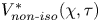
Figure 8 shows the profiles of isothermal and non‐isothermal gas velocity fields in C-1.43-50 as a function of depth into the granular column, $V_{iso}^\ast (\chi )$ and $V_{non\text{-}iso}^\ast (\chi )$, at times corresponding to figure 5. In contrast with the decaying profiles θ_iso(χ) and θ_non‐iso(χ), the profiles $V_{iso}^\ast (\chi )$ and $V_{non\text{-}iso}^\ast (\chi )$ both exhibit non-monotonic characteristics with singular velocity peaks formed at the very beginning of gas filtration. As the profiles $V_{iso}^\ast (\chi )$ and $V_{non\text{-}iso}^\ast (\chi )$ extend downstream with time, the downstream-moving velocity peak quickly flattens. After χ_s _,iso (and χ_s _,non‐iso) reaches the rear surface, a rear tail emerges and lifts up with time, indicating that the flows accelerate towards the rear surface. This phenomenon of flow acceleration is widely observed and attributed to the rapid fluid volume fraction changes across the rear surface, since the momentum and energy changes of the filtration flow due to the nozzling term (in (2.2) and (2.3)) become significant (Bdzil et al. Reference Bdzil, Menikoff, Son, Kapila and Stewart1999; Kalenko & Liberzon Reference Kalenko and Liberzon2020; Choi & Park Reference Choi and Park2022). Therefore, we describe the increase of fluid velocity caused by changes in volume fraction as the ‘nozzling effect’ in this paper. The rear-surface region across which the flows increasingly accelerate is denoted as RSR_acc.

Figure 8.

(a) Typical profiles of $V_{iso}^\ast (\chi )$ (dashed line) and $V_{non\text{-}iso}^\ast (\chi )$ (solid line) for C-1.43-50 during the unsteady and steady filtration phases. Unsteady phase: τ = 0.19, 0.78 and 2.29; steady phase: τ = 17.37. (b) Corresponding pressure gradient profiles, ∂χθ_iso(χ) and ∂χθ_non‐iso(χ), with markers indicating the locations of the velocity peaks.

For isothermal gas filtration, the correlation between the gas pressure and velocity is described by the Forchheimer resistance law (2.21). In the Darcy-flow domain, the Forchheimer resistance law reduces to the Darcy resistance law whereby the instantaneous gas velocity is proportional to the local pressure gradient. The velocity gradient depends on the quadratic differential of the pressure. Hence the profile $V_{iso}^\ast (\chi )$ peaks at the deflection point of the pressure gradient curve, ∂χθ_iso(χ), upon which ${\partial _\chi }V_{iso}^\ast (\chi )$ and $\partial _\chi ^2\theta _{iso}^\ast $ are zero. Similarly, the signature peak in the profile $V_{non\text{-}iso}^\ast (\chi )$ also arises from the deflection of ∂_χθ_non‐iso(χ). Indeed, the deflection points in profiles ∂_χθ_iso(χ) and ∂_χθ_non‐iso(χ) shown in figure 8(b) coincide with the locations of the peak summits of profiles $V_{iso}^\ast (\chi )$ and $V_{non\text{-}iso}^\ast (\chi )$, respectively.

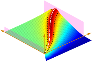
The temporospatial evolutions of the non‐isothermal and isothermal gas velocity fields for C-1.43-50 plotted in figure 9(a,b) show similar patterns. However, the non‐isothermal gas flows are considerably faster than the isothermal flows. Notably, the rear-surface acceleration for the non‐isothermal filtration is much more evident and affects the regions far removed from the rear surface. Accordingly, the rarefaction waves accompanying the development of the rear-surface accelerating flows are stronger in the non‐isothermal filtration, sufficing to cause the marked retraction of ${\theta _{non\text{-}iso}}(\chi ,\tau )$ contour lines in figure 7.

Figure 9.

Temporospatial evolutions of $V_{iso}^\ast (\chi ,\tau )$ (a) and $V_{non\text{-}iso}^\ast (\chi ,\tau )$ (b) for C-1.43-50 superimposed with the velocity isolines.

For compressible gas flows, the velocity fields are closely coupled with the thermodynamic parameters. Thus, to gain a thorough understanding of the thermodynamic parameters in the non‐isothermal gas filtration, the evolving flow characteristics need to be elucidated. Figure 10 shows the velocity profiles $V_{non\text{-}iso}^\ast (\chi )$ for a range of systems with M_s and Π spanning the entire parameter space. The first three profiles from left to right describe the streamwise velocity distributions at the moments of the filtration incipiency (χ_s _,non‐iso = 0.2), the half-column being infiltrated (χ_s _,non‐iso = 0.5) and the flows reaching the rear surface (χ_s _,non‐iso = 1). The fourth profile is the converged profile corresponding to the steady pressure diffusion phase.

Figure 10.

Successions of profiles $V_{non\text{-}iso}^\ast (\chi )$ for a range of systems with varying M_s and Π, displaying a complete evolution of velocity fields. The χ_s,non‐iso values corresponding to the first three profiles $V_{non\text{-}iso}^\ast (\chi )$ from left to right are 0.2, 0.5 and 1, represented by the solid black, the dashed blue and the dotted green lines, respectively. The fourth profile in the dashed-dotted red line represents the steady flow.

Although the progression of $V_{non\text{-}iso}^\ast (\chi )$ displayed in figure 10 exhibits a similar trend to that shown in figure 9(a), the influences from M_s and Π cause distinct flow characteristics, from very incipient unsteady flows to well-developed steady flow. As M_s increases the primary velocity peak in the incipient $V_{non\text{-}iso}^\ast (\chi )$ becomes increasingly prominent with an elevated amplitude and steepened declining slope. The peak amplitude is quantified by $\Delta V_{peak}^\ast= (V_{peak}^\ast - V_0^\ast )/V_0^\ast $, where $V_{peak}^\ast $ and $V_0^\ast $ represent the peak velocity and velocity at the front surface, respectively. Figure 11 shows the dependence of $\Delta V_{peak}^\ast $ on M_s with Π = 5 × 10⁻⁵, 0.5 and 5 × 10⁴. Here, $\Delta V_{peak}^\ast $ is calculated based on the profile $V_{non\text{-}iso}^\ast (\chi )$ with χ_s _,iso = 0.5. The M_s dependence of $\Delta V_{peak}^\ast $ demonstrates an asymptotic convergence trend regardless of Π varying over nine orders of magnitude, while $\Delta V_{peak}^\ast $ is negligible (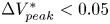$\Delta V_{peak}^\ast < 0.05$) in the weakest shock domain (M_s < 1.1).

Figure 11.

Variations in $\Delta V_{peak}^\ast $ with M_s. Inset: zoom-in plot of $\Delta V_{peak}^\ast ({M_s})$ in the weakest incident shock domain, M_s < 1.1.

Another striking flow characteristic associated with the increased M_s is the amplified tail rising of the velocity profile, indicating an enhanced rear-surface acceleration. Figure 12(a) shows a comparison of the profiles $V_{non\text{-}iso}^\ast (\chi )$ for the steady flows in systems with Π = 0.5 and increasing M_s; significant steepening and narrowing of the lifting tails are observed. Except for the lifting tail, the bulk of the velocity profiles can be effectively fitted by a linear function as indicated in figure 12(a). Thus, the point beyond which the extrapolated fitting line and the actual profile become non-trivial is considered to be the beginning point of the lifting tail, or equivalently the front edge of the RSR_acc and denoted by χ_RSR hereafter. The χ_RSR for systems with M_s = 1.43, 1.54, 1.83 and 2.22 is indicated in figure 12(a) and gradually moves downstream with increased M_s consistent with the narrowing trend of the lifting tail with M_s. The χ _RSR is not discernible in cases with the weakest incident shocks, such as M_s = 1.09 and 1.17. The tail rising rate ${\partial _\chi }V_{tail}^\ast $ is calculated as the average variation of V*(χ) per unit χ within the width of the RSR_acc, ΔRSR_acc, as follows:

(4.2)

\begin{equation}{\partial _\chi }V_{tail}^\ast= \frac{{V_{\chi = 1}^\ast- V_{{\chi _{RSR}}}^\ast }}{{V_{{\chi _{RSR}}}^\ast\,{\cdot}\, \mathrm{\Delta RS}{\textrm{R}_{acc}}}},\end{equation}

where $V_{\chi = 1}^\ast $ and $V_{{\chi _{RSR}}}^\ast $ represent the velocities at the rear surface and χ = χ_RSR, respectively, ΔRSR_acc = 1 − χ_RSR. Figure 12(b) shows the variations in χ_RSR and ${\partial _\chi }V_{tail}^\ast $ with increasing M_s and unvaried Π, Π = 0.5. The χ_RSR first quickly moves downstream as the incident shock transitions from weak to strong and then converges to ~0.7 after M_s > 2; this result indicates a lower limiting width of the RSR_acc, ΔRSR_acc = 0.3. Moreover, the tail rising rate ${\partial _\chi }V_{tail}^\ast $ continues to increase. From M_s = 1.4 to M_s = 3, ${\partial _\chi }V_{tail}^\ast $ increases almost tenfold.

Figure 12.

(a) Comparison of the profiles $V_{non\text{-}iso}^\ast (\chi )$ for the steady flows in systems with increasing M_s; the circle symbols indicate the front edges of the RSR_acc beyond which the linear fitted lines denoted by the dashed line start to deviate from the actual profiles. (b) The M_s dependence of the front edge of the RSR_acc, χ_RSR (left axis), and the tail rising rate, $\partial \chi V_{tail}^\ast $ (right axis).

4.3. Gas temperature

Figure 13(a) displays the temporospatial evolution of the non-dimensional temperature field, ${T^\ast } = T/{T_5}$, for C-1.43-50. Notably, there is a downstream-travelling hot gas layer whose temperature is considerably higher than T ₅ and continues to increase. The profiles T*(χ) at sequential times shown in figure 13(b) manifest the diffusive nature of the hot gas layer which spreads out while traversing the length of the column. The envelope of the peaks in the profiles T*(χ) indicated by the red curve in figure 13(b) shows the variation in the peak temperature $T_{peak}^\ast $ as a function of χ. For C-1.43-50, the hot gas layer undergoes a substantial self-heating phase until it travels midway through the column when $T_{peak}^\ast $ reaches its maximum $T_{max}^\ast $. The corresponding location of the temperature peak is denoted as ${\chi _{T_{max}^\ast }}$.

Figure 13.

(a) Temporospatial evolution of the non-dimensional temperature field T* for C-1.43-50. (b) Profiles T*(χ) at sequential times enveloped by the evolution line of $T_{peak}^\ast $ which reaches $T_{max}^\ast $ at $\chi = {\chi _{T_{max}^\ast }}$. At every moment, the position of the temperature peak, ${\chi _{T_{peak}^\ast }}$, coincides with the position of the contact surface particle, χ_CS.

The trajectory of the temperature peak, ${\chi _{T_{peak}^\ast }}$, is depicted in χ–τ space as indicated by the dashed line in figure 13(a). Another important trajectory is that of the contact surface, χ_CS, which separates the initial interstitial gases and infiltrated gases flowing from upstream. Note that the trajectory of the contact surface is actually the trace line of the first gas particle flowing into the granular column upon shock impingement. The derivation of χ_CS is presented in Appendix B. As shown in figure 13(b), the positions of ${\chi _{T_{peak}^\ast }}$ and χ_CS coincide with each other at every moment, implying that the temperature peak resides upon the contact surface, or equivalently it is the very first gas particle flowing into the column that is the hottest one. The coincidence between ${\chi _{T_{peak}^\ast }}(\tau )$ and χ_CS(τ) is further explored in § 4.4.

Two more distinct heating processes of the hot gas layers are shown in figure 14(a,b). For C-1.09-50 (see figure 14a), $T_{peak}^\ast $ increases to its maximum near the front surface, 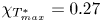${\chi _{T_{max}^\ast }} = 0.27$, followed by a gently declining plateau. In this scenario, most parts of the granular column are subjected to $T_{max}^\ast $ albeit the values of $T_{max}^\ast $ are modest, $T_{max}^\ast= 1.035$. In contrast, for C-2.22-0.045, the increase in $T_{peak}^\ast $ persists until the hot gas layer passes the rear surface, ${\chi _{T_{max}^\ast }} = 1$. We observe a singularly maximum temperature $T_{max}^\ast= 3.11$ at the rear surface.

Figure 14.

Profiles T*(χ) for C-1.09-50 (a) and C-2.22-0.045 (b). Envelopes of the temperature peaks at sequential times represent the variations in $T_{peak}^\ast $.

The traversing hot gas layer introduces additional energy into the gas filtration, part of which fuels the pressure diffusion. The coupling between the thermal effect embodied by the self-heating hot gas layer and the pressure diffusion is elaborated in § 4.4. The occurrence of thermal stress in granular materials exposed to rapid temperature changes is known as ‘thermal shock’. In fact, the propagation of the hot gas layer within the material induces a sharp thermal shock to the local solid skeleton with a temperature amplitude as high as a few hundred degrees. This intense thermal shock can result in significant surface or internal damages to the material, including cracks, fractures and other forms of degradation. For instance, a solid skeleton made of aluminium alloys loses almost its entire strength under thermal shock with an amplitude of 500 °C (Yin et al. Reference Yin, Ni, Liu, Fan, Zhi, Ye, Pan and Guo2023). Throughout the granular column the thermal shock markedly varies from part to part as indicated by the variation in $T_{peak}^\ast $ in figures 13(b) and 14, which causes a mismatch of the resulting thermal stresses and thermal expansion. The property degradation in combination with the mismatching thermal stresses poses a great threat to the structural integrity of the solid skeleton. Consequently, the shock resistance performance of the granular medium probably deteriorates. Therefore, the thermal resistance properties of porous materials as candidates for shock protection shields need to be among the primary concerns when assessing the overall shock resistance performance.

Parameters $T_{max}^\ast $ and ${\chi _{T_{max}^\ast }}$ are reasonable to use as the quantitative descriptors of the thermal effect of gas filtration. The former characterizes the intensity of the thermal effect while the latter measures the streamwise uniformity of the thermal effect. The contour maps of $T_{max}^\ast $, T_max and ${\chi _{T_{max}^\ast }}$ in the parameter space (M_s, Π) are shown in figure 15(a–c), respectively. A distinctive but resembling pattern can be identified from these contour maps. In general, a stronger incident shock causes a more intense and prolonged self-heating of the hot gas layer, especially in the strong incident shock domain M_s > 2. If we set the 10 % increase of the ambient temperature to 327.8 K as the upper limit of T_max below which the isothermal assumption holds, the corresponding threshold of M_s,iso is 1.08, as shown in figure 15(b). Note that the M_s dependences of $T_{max}^\ast $, T_max and ${\chi _{T_{max}^\ast }}$ are substantially amplified in the domain with strong shocks, M_s > 2, and median levels of Π, Π ~ O(10⁻³)–O(10⁻¹).

Figure 15.

Contour maps of $T_{max}^\ast $ (a), T_max (b) and ${\chi _{T_{max}^\ast }}$ (c) in the parameter space (M_s, Π). Three distinct heating modes, mode I: the gas-filtration-dominated mode, mode II: the rear-surface-dominated mode and mode III: persistent heating mode, are delineated by two boundaries. Boundaries between different modes are represented by the pink and white solid lines which are denoted as B-I-II and B-II-III, respectively.

In contrast with the monotonic increase in these parameters with M_s, the Π dependences are more complicated. In the domain of the weakest incident shock, M_s < 1.1, the isolines are parallel to the Π axis, indicating a minimum Π effect. As the incident shock strengthens, a nonlinear dependence of Π emerges and becomes increasingly prominent. For a given M_s (M_s > 1.8), $T_{max}^\ast $ and T_max reach their maxima in the neighbourhood of Π ~ O(10⁻²). Moreover, the completion of self-heating is delayed on the rear surface, ${\chi _{T_{max}^\ast }} = 1$. The resemblance of the variation patterns in $T_{max}^\ast $ and ${\chi _{T_{max}^\ast }}$ indicates an explicit correlation between the heating intensity and the duration for which self-heating occurs. Specifically, the delay of the temperature convergence corresponds to an elevated maximum temperature. The hot gas layer is able to obtain a higher $T_{max}^\ast $ if self-heating continually persists to the rear surface. In § 4.5, we further account for the variation in ${\chi _{T_{max}^\ast }}$ in the M_s–Π parameter space in terms of the heating modes.

4.4. Coupling between the thermal effect and the pressure diffusion

The influence of the thermal effect on the pressure diffusion depends on the amount of heat carried by the hot gas layer which can be converted into the pressure potential. The total heat and the conversion proportion both play a significant role. We employ the time integral of the heat flux passing through the rear surface as a measurement of the total heat. The heat flux at the rear surface, ${\dot{Q}_{rear}}$, is calculated as follows:

(4.3)

\begin{equation}{\dot{Q}_{rear}} = {\rho _{rear}}{e_{rear}}{V_{rear}},\end{equation}

where ρ_rear, e_rear and V_rear are the gas density, specific internal energy and gas velocity at the rear surface, respectively. Here e_rear is a function of the gas temperature at the rear surface, e_rear = c_vT_rear, where c_v is the constant-volume specific heat capacity. Substituting e_rear = c_vT_rear and the equation of state for the ideal gases, P_rear = ρ_rearRT_rear, into (4.3), (4.3) reduces to the following:

(4.4)

\begin{equation}{\dot{Q}_{rear}} = \frac{1}{{\gamma - 1}}{P_{rear}}{V_{rear}}.\end{equation}

Figure 16(a) shows evolution of ${\dot{Q}_{rear}}$ for C-1.43-50. When the diffusing pressure field front arrives at the rear surface, χ_p = 1 (t_diff _,non‐iso = 5.78 ms), ${\dot{Q}_{rear}}$ begins to increase until the contact surface particle passes through the rear surface (t_T = 72.0 ms) when ${\dot{Q}_{rear}}$ reaches the maximum. Afterwards the ${\dot{Q}_{rear}}$ curve drops slightly before converging to a steady value at t_heat = 85.3 ms. If we assume that thermal effect diminishes as the hot gas layer moves to the rear surface, the total heat relevant to the thermal effect, Q_heat, can be calculated as the integral of the ${\dot{Q}_{rear}}(t)$ curve from t_diff _,non‐iso to t_heat:

(4.5)

\begin{equation}{Q_{heat}} = \int_{{t_{diff\textrm{,}non\textrm{-}iso}}}^{{t_{heat}}} {{{\dot{Q}}_{rear}}\,\textrm{d}t} .\end{equation}

The contour map of Q_heat in the parameter space (M_s, Π) is shown in figure 16(b). The dependence of Q_heat on Π overpowers its dependence on M_s. Hence, the isolines exhibit a horizontally tilted pattern. As Π increases from O(10⁻⁵) to O(10⁴), Q_heat increases over five decades.

Figure 16.

(a) Temporal variation in ${\dot{Q}_{rear}}$ prior to a steady heat flux being established for C-1.43-50. (b) Contour map of Q_heat in the parameter space (M_s, Π).

The proportion of Q_heat contributing to pressure diffusion depends on the ratio between the traversal time of the hot gas layer, τ_T, and the characteristic time of the pressure diffusion, ξ_T = τ_T/τ_diff _,non‐iso. The contour map of ξ_T in the parameter space (M_s, Π) is shown in figure 17(a); a strong dependence on M_s in the weak incident shock domain, M_s < 1.6, is observed, and Π plays a more important role in the strong incident shock domain, M_s ≥ 1.6. Inside the upper right corner of the parameter space delineated by the isoline ξ_T = 1 (see figure 17a), the hot gas layer travels faster than the pressure diffusion; therefore, almost all Q_heat is available for expediting the pressure diffusion. Otherwise, the cumulative heat flux in the duration of τ_diff _,non‐iso possibly contributes to a faster pressure diffusion. The inverse of ξ_T serves as a scale factor measuring the proportion of Q_heat fuelling the pressure diffusion. The heat available for conversion into the pressure potential, Q_T→p, is a function of Q_heat as well as ξ_T:

(4.6)

\begin{equation}\left. {\begin{array}{@{}l@{}} {{Q_{T \to p}} = {Q_{heat}}\quad \textrm{for}\;{\xi_T} < 1,}\\ {{Q_{T \to p}} = {Q_{heat}}/{\xi_T}\quad \textrm{for}\;{\xi_T} \ge 1.} \end{array}} \right\}\end{equation}

Figure 17(b) shows the contour map of Q_T→p which has a similar pattern to Q_heat. Specifically, the isolines of Q_T→p take the form of a semi-parallel inclined line in the weak incident shock domain, M_s < 1.6, while they transition into a series of semi-horizontal lines in the strong incident shock domain, M_s ≥ 1.6.

Figure 17.

Contour maps of ξ_T (a), Q_T→p (b), E_p (c) and $Q_{T \to p}^\ast $ (d) in the parameter space (M_s, Π).

A non-dimensional Q_T→p, $Q_{T \to p}^\ast= {Q_{T \to p}}/{E_p}$, is employed to better characterize the thermal effects on the pressure diffusion, where E_p is the cumulative pressure potential energy along the length of the granular column subject to the steady diffusing pressure field:

(4.7)

\begin{equation}{E_p} = \int_0^l {P(x)\,\textrm{d}\kern0.7pt x} .\end{equation}

Figure 17(c) plots the contour map of E_p in the parameter space (M_s, Π) wherein the isolines take the form of regularly spaced parallel lines slowly inclining from the upper left towards the lower right. For C-1.43-50, 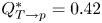$Q_{T \to p}^\ast= 0.42$ with Q_T→p = 1.37 × 10⁵ J m⁻² and E_p = 3.19 × 10⁵ J m⁻², indicating the heat available to fuel the pressure diffusion is 42 % of the pressure potential. The contour map of $Q_{T \to p}^\ast $ calculated as the ratio between Q_T→p and E_p is shown in figure 17(d); this displays convoluted isolines with the highest value $Q_{T \to p}^\ast{\sim} 0.7$ appearing in the region as Π approaches the upper limit, Π ~ O(10⁴), while the incident shock is relatively weak, M_s ~ 1.3. Notably, the bottom region of figure 17(d) enclosed by the isoline $Q_{T \to p}^\ast= 0.1$ roughly coincides with the upper boundary of TR_diff. Indeed, beneath the isoline $Q_{T \to p}^\ast= 0.1$, the heat flux contributing to diffusion is trivial relative to the pressure potential which is the primary driving force for diffusion. Accordingly, the pressure diffusion therein is barely affected.

4.5. Mechanisms underlying the thermal effect

In this section, the heating mechanism governing the temperature evolution of the traversing hot gas layer is accounted for from the perspective of energy conservation. In the Lagrangian frame, the internal energy conservation equation for an individual gas particle is as follows:

(4.8)

\begin{equation}{\rho _g}\frac{R}{{\gamma - 1}}\frac{{\textrm{d}T}}{{\textrm{d}t}} = \frac{{1 - \varepsilon }}{\varepsilon }{\rho _g}{D_p}V_g^2 - P\frac{{\partial {V_g}}}{{\partial x}}.\end{equation}

The term on the left-hand side of (4.8) represents the growth rate of the internal energy per unit volume. The variation in the internal energy is related to the viscous dissipation caused by the drag force between the gas and solid skeleton (the first term on the right-hand side) as well as unsteady pressure work (the second term on the right-hand side). Viscous dissipation always leads to gas heating. In contrast, the contribution of the pressure work to the gas internal energy depends on the sign of the streamwise velocity gradient. Specifically, accelerating gases undergoing expansion are doing work to the surroundings at the expense of the internal energy. Otherwise, decelerating gases are heated up along with being compressed. Thus, whether gas heating occurs depends on the nature (expansion or compression) and magnitude of the pressure work relative to viscous dissipation. Gas heating is terminated only when the gas particle commences a sufficiently strong acceleration phase. A maximum temperature is observed inside the granular column. Otherwise, the gas particle's temperature continuously increases until it passes through the rear surface.

To better illustrate the dependence of the thermal effect on the flow and thermodynamic parameters, we substitute the drag force model, namely the Di Felice model ((2.4)–(2.7)), and the non-dimensional variables defined in (2.20) into (4.8). Hence, (4.8) reduces to its non-dimensional form:

(4.9)

\begin{equation}\begin{array}[b]{@{}l@{}} \dfrac{{\textrm{d}{T^\ast }}}{{\textrm{d}\tau }} = \dfrac{{N(\gamma - 1)}}{{N + 1}}\dfrac{{{\mu ^\ast }}}{{\rho _{non\textrm{-}iso}^\ast }}{(V_{non\textrm{-}iso}^\ast )^2} + \dfrac{{N(\gamma - 1)}}{{N + 1}}N\Pi \dfrac{{{\rho _5}}}{{{\rho _1}}}{(V_{non\textrm{-}iso}^\ast )^3}\\ \phantom{\dfrac{{\textrm{d}{T^\ast }}}{{\textrm{d}\tau }} = } - \dfrac{{N{\theta _{non\textrm{-}iso}} + 1}}{{N + 1}}\dfrac{{\gamma - 1}}{{\rho _{non\textrm{-}iso}^\ast }}\dfrac{{\partial V_{non\textrm{-}iso}^\ast }}{{\partial \chi }}, \end{array}\end{equation}

where μ* is the non-dimensional dynamic viscosity, μ* = μ_g/μ ₁, and the non-dimensional density ρ* satisfies the non-dimensional equation of state for ideal gases:

(4.10)

\begin{equation}\rho _{non\textrm{-}iso}^\ast= \frac{{N{\theta _{non\textrm{-}iso}} + 1}}{{N + 1}}\frac{1}{{{T^\ast }}}.\end{equation}

The first and second terms on the right-hand side of (4.9) represent the (linear) viscous and (nonlinear) inertial losses of the viscous dissipation, respectively. As indicated in (4.9), the variation rate of the gas temperature depends on the instantaneous values of the velocity, $V_{non\textrm{-}iso}^\ast $, the velocity gradient, ${\partial _\chi }V_{non\textrm{-}iso}^\ast $, the pressure, θ_non‐iso, and the density, $\rho _{non\textrm{-}iso}^\ast $.

For low-speed gas filtration without the compressible effect, the gaseous density $\rho _{non\textrm{-}iso}^\ast $ remains consistent from the upstream all the way down to the downstream. As a result, T* is proportional to θ_non‐iso which monotonically decays with distance from the upstream surface. Thus, no gas heating is expected. For isothermal gas filtration with the compressible effect which does not allow the upstream temperature to differ from the downstream one, there is no temperature variation (dT*/dτ = 0). Equation (4.9) reduces to the compressible version of the Forchheimer law, whereby the linear and nonlinear flow resistance forces as well as the unsteady pressure work are all taken into account.

We first address the non-existence of the thermal effect during the steady pressure diffusion phase during which the temperature field is uniform and consistent with T ₅. As illustrated in figure 10, the converged velocity profile, $V_{non\textrm{-}iso}^\ast (\chi )$, of the steady flows has a form of a gently upwards slope with (in the strong incident shock domain) or without (in the weak incident shock domain) a lifting tail. The overall low magnitude and flatness of the profile $V_{non\textrm{-}iso}^\ast (\chi )$ except for the lifting tail indicate that the gas particles flow through the bulk of the granular column at relatively low and unvaried velocities. Hence, outside the RSR_acc all three terms on the right-hand side of (4.9) become negligible such that the gas temperature remains constant. If the profile $V_{non\textrm{-}iso}^\ast (\chi )$ features a significant lifting tail, the gas particles undergo a substantial acceleration as they pass through the RSR_acc, and the viscous dissipation and the expansion work are equally intense such that the resulting heating and cooling effects may be effectively negated. As a result, the gas temperature barely changes across the RSR_acc. Figure 18 shows the streamwise variations in each of the three terms on the right-hand side of (4.9) during the steady diffusion phase for C-2.99-5000 which is supposed to manifest the strongest thermal effect. The viscous loss (the first term) of the viscous dissipation remains minimal which is consistent with the Forchheimer flow characteristic of gas filtration in this case with Re_f = 2.5 × 10⁵. The inertial loss and pressure work terms, albeit having non-trivial values, offset each other due to opposite signs leading to a neutralized temperature growth rate as shown in figure 18(b). No thermal effect in terms of detectable heating or cooling effects can be observed during the steady filtration phase.

Figure 18.

(a) Zoom-in plot (χ > 0.9) of the streamwise variations in the viscous loss, inertial loss and pressure work during the steady diffusion phase for C-2.99-5000. Inset: the whole streamwise profiles of each term. (b) Corresponding temperature growth rate and temperature distribution along the length of the granular column.

In contrast to the steady flows during the steady filtration phase, gas particles flow through the column at relatively high and markedly varying velocities during the incipient filtration phase as indicated in figure 10. Accordingly, the viscous dissipation and the pressure work in this phase play a non-trivial role, producing intensified thermal effects. The very first gas particle that flows into the granular column upon shock impingement, namely the contact surface particle, attains the highest velocities and undergoes the most significant velocity fluctuation. Figure 19(a–c) shows a comparison of the velocity evolutions of the contact surface particle, $V_{CS}^\ast (\chi )$, and the converged velocity profiles for C-1.09-50, C-2.22-50 and C-2.22-0.045, respectively; considerable differences, especially in the first half of the column, are observed. Consequently, the contact surface particle is subjected to the most intensified heating. The trace line of the contact surface particle forms the hottest contour line in the temperature field T* as shown in figure 13(a).

Figure 19.

Comparisons of the contact surface particle's velocity evolutions $V_{CS}^\ast (\chi )$ and converged velocity profiles $V_{non\text{-}iso}^\ast (\chi )$ for C-1.09-50 (a), C-2.22-50 (b) and C-2.22-0.045 (c). Profile $V_{CS}^\ast (\chi )$ for C-0.5-50 deflects upon the steady diffusing pressure fields is established and marked by the red circle in (a). The front edges of the RSR_acc for C-2.22-50 and C-2.22-0.045 are also indicated in (b,c) by χ_RSR. Profiles $T_{CS}^\ast (\chi )$ corresponding to (a–c) are shown in (d–f), respectively. The locations of $T_{max}^\ast (\chi )$ are denoted by ${\chi _{T_{max}^\ast }}$ marked in each panel.

For C-1.09-50 the temperature of the contact surface particle, $T_{CS}^\ast (\chi )$, reaches its maximum at the deflection point of the profile $V_{CS}^\ast (\chi )$ as shown in figure 19(d), 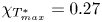${\chi _{T_{max}^\ast }} = 0.27$. Actually, the $V_{CS}^\ast (\chi )$ curve beyond 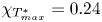${\chi _{T_{max}^\ast }} = 0.24$ coincides with the converged velocity profile since the steady flows are well developed when the contact surface particle reaches ${\chi _{T_{max}^\ast }}$. Gas self-heating is terminated by the premature formation of the steady flows, which occur in cases where the filtrated gas particles lag far behind the pressure diffusion front, ξ_T ~ O(10¹). Since there is no gas acceleration towards the rear surface, we refer to this heating mode as the gas-filtration-dominated mode.

For C-2.22-50 and C-2.22-0.045, both of which have noticeable RSR_acc, the maximum temperatures of the contact surface particles are attained at the front edge of RSR_acc, ${\chi _{T_{max}^\ast }} = {\chi _{RSR}}$, and the rear surface, ${\chi _{T_{max}^\ast }} = 1$, respectively. Since the heating effect associated with the viscous dissipation and the ‘cooling effect’ caused by the expansion work are both active inside the RSR_acc, ${\chi _{T_{max}^\ast }} = {\chi _{RSR}}$ indicates that the cooling effect prevails while ${\chi _{T_{max}^\ast }} = 1$ means that the heating effect dominates throughout. The cases wherein the cooling effect inside the RSR_acc suffices to reverse the persistent gas heating, such as C-2.22-50, are referred to as the rear-surface-dominated heating mode. Otherwise, the gases are continually heated to the rear surface in cases such as C-2.22-0.045, which are referred to as the persistent heating mode.

The boundaries delineating these three distinct heating modes are superimposed on the contour map of ${\chi _{T_{max}^\ast }}$ in figure 15(c). The boundary between the gas-filtration- and rear-surface-dominated modes roughly aligns with the vertical line M_s ~ 1.4 which coincides with the isoline of ξ_T = 2 as indicated in figure 17(a). In the gas-filtration-dominated domain the gas temperature reaches $T_{max}^\ast $ in the first half of the granular column and gradually decreases as the gases flow downstream. The persistent heating mode resides in the narrow band enveloped by the vertical line M_s ~ 1.8, and two horizontal lines Π ~ 10⁻² and Π ~ 10⁻¹. The remaining region in the M_s–Π space belongs to the rear-surface-dominated domain, where $T_{max}^\ast $ is reached inside the RSR_acc. Upon closer inspection of figure 15(a,c), the presence of the persistent heating domain evidently warps the contour lines of $T_{max}^\ast $ and T_max therein such that $T_{max}^\ast (\varPi )$ and T_max(Π) display significant nonlinear behaviours across the persistent heating domain.

The location of the persistent heating domain in the parameter space (M_s, Π) can be predicted via (4.9). The viscous loss (first term on the right-hand side), the inertial loss (second term on the right-hand side) and the pressure work (third term on the right-hand side) scale with ${(V_{non\textrm{-}iso}^\ast )^2}$, 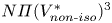$N\varPi {(V_{non\textrm{-}iso}^\ast )^3}$ and ${\partial _\chi }V_{non\textrm{-}iso}^\ast $, respectively. Employing $V_{{\chi _{RSR}}}^\ast $ and the average gradient of V*(χ) within ΔRSR_acc as approximations of $V_{non\textrm{-}iso}^\ast $ and ${\partial _\chi }V_{non\textrm{-}iso}^\ast $, respectively, gives the following:

(4.11)

\begin{equation}{\partial _\chi }V_{non\textrm{-}iso}^\ast= \frac{{\partial V_{non\textrm{-}iso}^\ast }}{{\partial \chi }} = \frac{{V_{\chi = 1}^\ast- V_{{\chi _{RSR}}}^\ast }}{{\Delta \textrm{RS}{\textrm{R}_{acc}}}}.\end{equation}

We plot each term's variations with Π at M_s = 1.43 and 2.22 as shown in figure 20(a,b). For both cases the viscous loss overwhelms the inertial loss in the domain with Π ≤ O(10⁻¹) and Re_f ≤ O(10⁰) corresponding to the Darcy flow regime. As Π exceeds O(10⁻¹), the Forchheimer flow begins to develop, and the inertial loss becomes dominant. Hence, whether gas self-heating is sustained across RSR_acc (dT*/dτ > 0) depends on the relative importance of the pressure work and the viscous loss (Π ≤ O(10⁻¹)) or the inertial loss (Π > O(10⁻¹)). For the strong incident shock, M_s = 2.22, the value of viscous loss exceeding the absolute value of the (expansion) pressure work only occurs within a narrow interval of Π, O(10⁻²) < Π < O(10⁻¹) (see figure 19a), wherein the persistent heating mode dominates. Beyond this interval of Π, the pressure work always prevails over either the viscous loss (Π ≤ O(10⁻¹)) or the inertial loss (Π > O(10⁻¹)). The gas heating is halted within the RSR_acc. The rear-surface-dominant heating mode is also the sole heating mode for M_s = 1.43 regardless of Π since the pressure work inside the RSR_acc is always higher than the viscous and internal losses (see figure 20b). The predicted location of the persistent heating domain in the parameter space (M_s, Π) is consistent with the numerically derived phase diagram shown in figure 15(a).

Figure 20.

Variations in the magnitudes of the viscous loss, inertial loss and pressure work with Π at M_s = 1.43 (a) and 2.22 (b). Inset of (b): zoom-in plot of the variations in magnitude of each term in the domain with Π ≤ O(10⁻¹).

5. Discussion

The relation between the non‐isothermal gas density, $\rho _{non\textrm{-}iso}^\ast $, and the non‐isothermal temperature, $T_{non\textrm{-}iso}^\ast $, as well as the non‐isothermal pressure, θ_non‐iso, is shown in (4.10). Differentiating (4.10) with respect to χ enables the correlation of the spatial variation of $\rho _{non\textrm{-}iso}^\ast $ with $T_{non\textrm{-}iso}^\ast $ and θ_non‐iso as given in (5.1):

(5.1)

\begin{align}\frac{{\partial \rho _{non\textrm{-}iso}^\ast }}{{\partial \chi }} = \frac{1}{{(N + 1)T{{_{non\textrm{-}iso}^\ast }^2}}}\left[ {NT_{non\textrm{-}iso}^\ast \frac{{\partial {\theta_{non\textrm{-}iso}}}}{{\partial \chi }} - (N{\theta_{non\textrm{-}iso}} + 1)\frac{{\partial T_{non\textrm{-}iso}^\ast }}{{\partial \chi }}} \right].\end{align}

Since θ_non‐iso monotonically decays with χ, ∂_χθ_non‐iso < 0 and whether $\rho _{non\textrm{-}iso}^\ast $ similarly decays with χ depends on the sign and magnitude of ${\partial _\chi }T_{non\textrm{-}iso}^\ast $. Note that the coefficients in the two derivative terms on the right-hand side of (5.1), $NT_{non\textrm{-}iso}^\ast $ and Nθ_non‐iso + 1, are of the same order of magnitude. Figure 21 shows the characteristic profiles $\rho _{non\textrm{-}iso}^\ast $ and $T_{non\textrm{-}iso}^\ast (\chi )$ for C-3.5-50 at τ = 1.45. On the rising side of the temperature peak, ${\partial _\chi }T_{non\textrm{-}iso}^\ast > 0$ such that $\rho _{non\textrm{-}iso}^\ast $ decreases with χ with a steeper slope than that of the isothermal density. On the declining side of the temperature peak, ${\partial _\chi }T_{non\textrm{-}iso}^\ast < 0$. If the absolute value of ${\partial _\chi }T_{non\textrm{-}iso}^\ast $, $|{{\partial_\chi }T_{non\textrm{-}iso}^\ast } |$, is in excess of that of ∂_χθ_non‐iso, ${\partial _\chi }\rho _{non\textrm{-}iso}^\ast $ becomes positive, resulting in a temporary increase in $\rho _{non\textrm{-}iso}^\ast $. As shown in figure 21(a) a depression appears in profile $\rho _{non\textrm{-}iso}^\ast (\chi )$ immediately downstream of the temperature peak, wherein $|{{\partial_\chi }T_{non\textrm{-}iso}^\ast } |$ is the largest. The $|{{\partial_\chi }T_{non\textrm{-}iso}^\ast } |$ becomes increasingly smaller with χ as the tail of the profile $T_{non\textrm{-}iso}^\ast (\chi )$ spreads out and eventually is surpassed by $|{{\partial_\chi }{\theta_{non\textrm{-}iso}}} |$. Afterwards the profile $\rho _{non\textrm{-}iso}^\ast (\chi )$ resumes the general decay characteristics.

Figure 21.

(a) Profiles of $\rho _{non\textrm{-}iso}^\ast $ (blue dashed line), $T_{non\textrm{-}iso}^\ast (\chi )$ (red solid line) and $\theta _{non\textrm{-}iso}^\ast (\chi )$ (black dash-dot line) for C-3.5-50 at τ = 1.45. The shaded band indicates the region with a positive density gradient, $\partial \chi \rho _{non\text{-}iso}^\ast > 0$. (b) Streamwise variations in the width and amplitude of the positive $\partial \chi \rho _{non\text{-}iso}^\ast $ phase, $\Delta {\chi _{\partial \rho > 0}}$ and $\Delta \rho _{\partial \rho > 0}^\ast $ for C-3.5-50.

The emergence of the evident temperature peak in the profile $T_{non\textrm{-}iso}^\ast (\chi )$ is the signature of the thermal effects. As mentioned before, the density depression in the profile $\rho _{non\textrm{-}iso}^\ast (\chi )$ is also the imprint of the thermal effects. The width and amplitude of the rising ramp of the density depression with positive ${\partial _\chi }\rho _{non\textrm{-}iso}^\ast $ show the influence of the thermal effects on the density field. We denote the starting and ending points of the positive ${\partial _\chi }\rho _{non\textrm{-}iso}^\ast $ phase as $\chi _{\partial \rho > 0}^0$ and $\chi _{\partial \rho > 0}^1$, respectively. The width of the positive ${\partial _\chi }\rho _{non\textrm{-}iso}^\ast $ phase, $\Delta {\chi _{\partial \rho > 0}}$, is the interval between $\chi _{\partial \rho > 0}^0$ and $\chi _{\partial \rho > 0}^1$, $\Delta {\chi _{\partial \rho > 0}} = \chi _{\partial \rho > 0}^1 - \chi _{\partial \rho > 0}^0$. The amplitude of the positive ${\partial _\chi }\rho _{non\textrm{-}iso}^\ast $ phase is defined as $\Delta \rho _{\partial \rho > 0}^\ast= \rho _{non\textrm{-}iso}^\ast (\chi _{\partial \rho > 0}^1) - \rho _{non\textrm{-}iso}^\ast (\chi _{\partial \rho > 0}^0)$. Figure 21(b) shows the streamwise variations in $\Delta {\chi _{\partial \rho > 0}}$ and $\Delta \rho _{\partial \rho > 0}^\ast $ for C-3.5-50. As this case belongs to the rear-surface-dominated heating mode domain, the temperature peak becomes tempered inside the RSR_acc, indicating the waning of the thermal effects. As a result, the positive ${\partial _\chi }\rho _{non\textrm{-}iso}^\ast $ phase becomes increasingly narrower with reduced amplitude as shown in figure 21(b).

Figure 22(a–c) displays the temporospatial evolutions of $\rho _{non\textrm{-}iso}^\ast $ in C-1.09-50, C-1.43-50 and C-2.22-0.045, which belong to the gas-filtration-dominated, rear-surface- dominated and persistent heating domains, respectively. The temporospatial evolutions of the corresponding ${\partial _\chi }\rho _{non\textrm{-}iso}^\ast $ are shown in figure 22(d–f), respectively. The thermal effect in the gas-filtration-dominated heating mode is generally modest, shown by the slight temperature rise, as indicated in figure 14; this does not suffice to cause a positive ${\partial _\chi }\rho _{non\textrm{-}iso}^\ast $ phase, which is the case in C-1.09-50 (figure 22a,d). The amplified thermal effect in the rear-surface-dominated heating mode allows the presence of a positive ${\partial _\chi }\rho _{non\textrm{-}iso}^\ast $ phase downstream of the contact surface (figure 22b,e). However, the positive ${\partial _\chi }\rho _{non\textrm{-}iso}^\ast $ phase diminishes as it approaches the rear surface since the thermal effect attenuates in the RSR_acc. We observe a substantial enhancement of the positive ${\partial _\chi }\rho _{non\textrm{-}iso}^\ast $ phase in cases controlled by the persistent heating mode in terms of the intensity, expanse and outreach, as shown in figure 22. A sharp density gradient across the hot gas layer enables high-speed schlieren imaging to visualize the thermal effect in this scenario.

Figure 22.

Temporospatial evolutions of $\rho _{non\text{-}iso}^\ast $ (a–c) and $\partial \chi \rho _{non\text{-}iso}^\ast $ (d–f) in C-1.09-50 (a,d), C-1.43-50 (b,e) and C-2.22-0.045 (c,f).

The misalignment of contour lines between θ_non‐iso and $\rho _{non\textrm{-}iso}^\ast $ provides the source for the baroclinic torque, $\boldsymbol{\nabla }{\theta _{non\textrm{-}iso}} \times \nabla \rho_{non\textrm{-}iso}^\ast $, which contributes to vorticity generation. If the vortices become so profuse that the laminar flow assumption is challenged, the formulations of Morrison's method become problematic. For mobile particle packings, the baroclinic vorticity introduces momentum to the particles in the non-streamwise directions and is likely responsible for the clustering or ‘channelling’ of the particles through the vortices. The baroclinic vorticity caused by thermal effects needs to be considered in the theory of shock-driven multiphase instability, which primarily accounts for the drag-induced vorticity deposition.

6. Conclusion

We carried out a comprehensive numerical investigation of shock-induced gas filtration through rigid granular columns in parameter space constructed by two defining non-dimensional parameters, namely the incident shock Mach number, M_s, and the filtration coefficient, Π. In contrast to the normally adopted isothermal gas filtration assumption, the results show an intense non‐isothermal filtration process characterized by a self-heating gas layer traversing the column. The resulting thermal effects have two major implications. First, the pressure diffusion is accelerated due to the influx of the additional heat which depends on the cumulative heat flux and the time-scale ratio between the thermal effect and the pressure diffusion. Second, the heat spike associated with the hot gas layer results in an intense thermal shock which may pose a threat to the integrity of the solid skeleton. The maximum gas temperature and the corresponding location are of most concern in this regard; they are used to characterize the intensity and uniformity of the thermal effect, respectively. The contour maps of the thermal effects are constructed in the parameter space (M_s, Π) from these two perspectives.

The self-heating mechanisms of the hot gas layer are considered in energy analysis. The thermal effects are further classified into three distinct modes based on the dominant heat mechanisms: gas-filtration-dominated, rear-surface-dominated and persistent heating modes. The phase diagram of the heating modes is also established in the parameter space (M_s, Π). Each heating mode correlates with distinct characteristics of the thermal effects, which justifies the variations in the thermal effects with M_s and Π.

Glossary

English letters

Greek letters

Subscripts

Declaration of interests

The authors report no conflict of interest.

Appendix A. Parameters in each numerical case

Four primary variables are involved in our simulations: the Mach number of the incident shock, M_s, the particle diameter, d_p, the packing fraction of the particle column, ϕ ₀, and the length of the column, l. With increasing Mach number from 1.094 to 2.986, the non-dimensional reflected shock intensity, N, introduced in (2.15) varies from 0.5 to 50. The other three variables constitute the filtration coefficient, Π. Since Π is mainly controlled by the particle diameter according to (2.18), d_p varies from 1 μm to 10 mm to ensure a wide variation range of Π. The packing fraction and particle column length contribute relatively less to Π; therefore, ϕ ₀ and l only vary within narrow ranges, ϕ ₀ from 0.45 to 0.58 and l/d_p from 200 to 1000. The exact values of the variable parameters in each case are provided in table 1.

Table 1.

Exact values of the variable parameters in each numerical case. The Mach number, M_s, and corresponding shock intensity, N, are provided in the first row, while the particle diameter, d_p, and corresponding filtration coefficient, Π, are given in the first column. The packing fraction and the length of the particle column are represented in the following order: ϕ ₀–l/d_p.

Appendix B. Approach to obtain the trajectory of the contact surface

The trajectory of the contact surface, χ _CS, is the moving route of the first gas particle flowing into the granular column upon shock impingement which can be obtained from the gas velocity field shown in figure 9. The new position of this gas particle along the flow direction can be updated from its previous position and the corresponding local gas velocity, as depicted in figure 23. Therefore, the complete trajectory of the contact surface is expressed as follows:

(B.1)

\begin{equation}\; {\chi _{CS}}(\tau ) = \int_0^\tau {V_{CS}^\ast \,\textrm{d}\tau } .\end{equation}

Figure 23.

Schematic diagram of the process to obtain the trajectory of the contact surface.

References

Abidoye, L.K., Khudaida, K.J. & Das, D.B. 2015 Geological carbon sequestration in the context of two-phase flow in porous media: a review. Crit. Rev. Environ. Sci. Technol. 45, 1105–1147.CrossRef Google Scholar

Alobaid, F. & Epple, B. 2013 Improvement, validation and application of CFD/DEM model to dense gas–solid flow in a fluidized bed. Particuology 11, 514–526.CrossRef Google Scholar

Apte, S., Mahesh, K. & Lundgren, T. 2003 A Eulerlan-Lagrangian model to simulate two-phase/particulate flows. Center for Turbulence Research Annual Research Briefs, pp. 161–171.Google Scholar

Baer, M.R. & Nunziato, J.W. 1986 A two-phase mixture theory for the deflagration-to-detonation transition (DDT) in reactive granular materials. Intl J. Multiphase Flow 12, 861–889.CrossRef Google Scholar

Balachandar, S. 2012 Recent advances in compressible multiphase flows explosive dispersal of particles. In Future Directions in CFD Research, a Modeling and Simulation Conference, Hampton.Google Scholar

Bdzil, J.B., Menikoff, R., Son, S.F., Kapila, A.K. & Stewart, D.S. 1999 Two-phase modeling of deflagration-to-detonation transition in granular materials: a critical examination of modeling issues. Phys. Fluids 11, 378–402.CrossRef Google Scholar

Bear, J. & Alexander, H.-D.C. 2010 Modeling Groundwater Flow and Contaminant Transport, 1st edn. Springer.CrossRef Google Scholar

Ben-Dor, G., Britan, A., Elperin, T., Igra, O. & Jiang, J.P. 1997 Experimental investigation of the interaction between weak shock waves and granular layers. Exp. Fluids 22, 432–443.CrossRef Google Scholar

Ben-Dor, G., Mazor, G., Igra, O., Sorek, S. & Onodera, H. 1994 Shock wave interaction with cellular materials. Shock Waves 3, 167–179.CrossRef Google Scholar

Borchardt-Ott, W. 2012 Crystallography: An Introduction. Springer.CrossRef Google Scholar

Britan, A., Ben-Dor, G., Elperin, T., Igra, O. & Jiang, J.P. 1997 Gas filtration during the impact of weak shock waves on granular layers. Intl J. Multiphase Flow 23, 473–491.CrossRef Google Scholar

Britan, A., Ben-Dor, G., Igra, O. & Shapiro, H. 2001 Shock waves attenuation by granular filters. Intl J. Multiphase Flow 27, 617–634.CrossRef Google Scholar

Britan, A., Ben-Dor, G., Igra, O. & Shapiro, H. 2006 Development of a general approach for predicting the pressure fields of unsteady gas flows through granular media. J. Appl. Phys. 99, 093519.CrossRef Google Scholar

Britan, A., Shapiro, H. & Ben-Dor, G. 2007 The contribution of shock tubes to simplified analysis of gas filtration through granular media. J. Fluid Mech. 586, 147–176.CrossRef Google Scholar

Britan, A., Shapiro, H., Liverts, M., Ben-Dor, G., Chinnayya, A. & Hadjadj, A. 2013 Macro-mechanical modelling of blast wave mitigation in foams. Part I. Review of available experiments and models. Shock Waves 23, 5–23.CrossRef Google Scholar

Carmouze, Q., Saurel, R., Chiapolino, A. & Lapebie, E. 2020 Riemann solver with internal reconstruction (RSIR) for compressible single-phase and non-equilibrium two-phase flows. J. Comput. Phys. 408, 109176.CrossRef Google Scholar

Chiapolino, A. & Saurel, R. 2020 Numerical investigations of two-phase finger-like instabilities. Comput. Fluids 206, 104585.CrossRef Google Scholar

Choi, D. & Park, H. 2022 Flow–structure interaction of a starting jet through a flexible circular nozzle. J. Fluid Mech. 949, A39.CrossRef Google Scholar

Crowe, C.T., Schwarzkopf, J.D., Sommerfeld, M. & Tsuji, Y. 2012 Multiphase Flows with Droplets and Particles. CRC Press.Google Scholar

De Paoli, M., Zonta, F. & Soldati, A. 2016 Influence of anisotropic permeability on convection in porous media: implications for geological CO₂ sequestration. Phys. Fluids 28, 056601.CrossRef Google Scholar

Del Prete, E., Chinnayya, A., Domergue, L., Hadjadj, A. & Haas, J.F. 2013 Blast wave mitigation by dry aqueous foams. Shock Waves 23, 39–53.CrossRef Google Scholar

Di Felice, R. 1994 The voidage function for fluid-particle interaction systems. Intl J. Multiphase Flow 20, 153–159.CrossRef Google Scholar

Ergun, S. 1952 Fluid flow through packed columns. Chem. Engng Prog. 48, 89–94.Google Scholar

Eriksen, F.K., Toussaint, R., Turquet, A.L., Måløy, K.J. & Flekkøy, E.G. 2018 Pressure evolution and deformation of confined granular media during pneumatic fracturing. Phys. Rev. E 97, 012908.CrossRef Google Scholar PubMed

Feng, Y., Xu, B., Zhang, S., Yu, A. & Zulli, P. 2004 Discrete particle simulation of gas fluidization of particle mixtures. AIChE J. 50, 1713–1728.CrossRef Google Scholar

Flekkøy, E.G., Sandnes, B. & Måløy, K.J. 2023 Shape of a frictional fluid finger. Phys. Rev. Fluids 8, 114302.CrossRef Google Scholar

Frost, D.L. 2018 Heterogeneous/particle-laden blast waves. Shock Waves 28, 439–449.CrossRef Google Scholar

Gubin, S.A. 2018 Shock waves in porous media J. Phys.: Conf. Ser. 1099, 012015.Google Scholar

Guo, Y., Wassgren, C., Hancock, B., Ketterhagen, W. & Curtis, J. 2015 Computational study of granular shear flows of dry flexible fibres using the discrete element method. J. Fluid Mech. 775, 24–52.CrossRef Google Scholar

Gvozdeva, L., Faresov, Y.M. & Fokeev, V. 1985 Interaction between air shock wave and porous compressible material. Sov. Phys. Appl. Math. Tech. Phys. 3, 111–115.Google Scholar

Han, P., Xue, K. & Bai, C. 2021 Explosively driven dynamic compaction of granular media. Phys. Fluids 33, 023309.CrossRef Google Scholar

Hayek, M. 2017 A model for subsurface oil pollutant migration. Transp. Porous Media 120, 373–393.CrossRef Google Scholar

Henderson, L., Virgona, R., Di, J. & Gvozdeva, L. 1990 Refraction of a normal shock wave from nitrogen into polyurethane foam. AIP Conf. Proc. 208, 814–818.CrossRef Google Scholar

Ji, S., Li, P. & Chen, X. 2012 Experiments on shock-absorbing capacity of granular matter under impact load. Acta Phys. Sin. 61, 184703–184703.Google Scholar

Jiang, Y., Guo, Y., Yu, Z., Hua, X., Lin, J., Wassgren, C.R. & Curtis, J.S. 2021 Discrete element method-computational fluid dynamics analyses of flexible fibre fluidization. J. Fluid Mech. 910, A8.CrossRef Google Scholar

Kafui, K.D., Thornton, C. & Adams, M.J. 2002 Discrete particle-continuum fluid modelling of gas–solid fluidised beds. Chem. Engng Sci. 57, 2395–2410.CrossRef Google Scholar

Kalenko, S. & Liberzon, A. 2020 Particle-turbulence interaction of high Stokes number irregular shape particles in accelerating flow: a rocket-engine model. Intl J. Multiphase Flow. 133, 103451.CrossRef Google Scholar

Koneru, R.B., Rollin, B., Durant, B., Ouellet, F. & Balachandar, S. 2020 A numerical study of particle jetting in a dense particle bed driven by an air-blast. Phys. Fluids 32, 093301.CrossRef Google Scholar

Kruggel-Emden, H., Sturm, M., Wirtz, S. & Scherer, V. 2008 Selection of an appropriate time integration scheme for the discrete element method (DEM). Comput. Chem. Engng 32, 2263–2279.CrossRef Google Scholar

Lage, J.L. 1998 The fundamental theory of flow through permeable media. From Darcy to turbulence. In Transport Phenomena in Porous Media (eds. Ingham, D.B. & Pop, I.), pp. 1–30. Pergamon.Google Scholar

Levy, A., Ben-Dor, G., Skews, B.W. & Sorek, S. 1993 Head-on collision of normal shock waves with rigid porous materials. Exp. Fluids 15, 183–190.CrossRef Google Scholar

Li, J., Xue, K., Zeng, J., Tian, B. & Guo, X. 2021 Shock-induced interfacial instabilities of granular media. J. Fluid Mech. 930, A22.Google Scholar

Li, J., Zeng, J. & Xue, K. 2023 Pressure evolution in shock-compacted granular media. Pet. Sci. 20, 3736–3751.CrossRef Google Scholar

Liu, X., Osher, S. & Chan, T. 1994 Weighted essentially non-oscillatory schemes. J. Comput. Phys. 115, 200–212.CrossRef Google Scholar

Meng, B., Zeng, J., Tian, B., Li, L., He, Z. & Guo, X. 2019 Modeling and verification of the Richtmyer–Meshkov instability linear growth rate of the dense gas-particle flow. Phys. Fluids 31, 074102.CrossRef Google Scholar

Mo, H., Lien, F.S., Zhang, F. & Cronin, D.S. 2019 A mesoscale study on explosively dispersed granular material using direct simulation. J. Appl. Phys. 125, 214302.CrossRef Google Scholar

Morrison, F.A. 1972 Transient gas flow in a porous column. Ind. Engng Chem. Res. Fundam. 11, 191–197.CrossRef Google Scholar

O'Rourke, P.J. & Snider, D.M. 2010 An improved collision damping time for MP-PIC calculations of dense particle flows with applications to polydisperse sedimenting beds and colliding particle jets. Chem. Engng Sci. 65, 6014–6028.CrossRef Google Scholar

Osnes, A.N., Vartdal, M. & Pettersson Reif, B.A. 2017 Numerical simulation of particle jet formation induced by shock wave acceleration in a Hele-Shaw cell. Shock Waves 28, 451–461.CrossRef Google Scholar

Patankar, N.A. & Joseph, D.D. 2001 Modeling and numerical simulation of particulate flows by the Eulerian-Lagrangian approach. Intl J. Multiphase Flow 27, 1659–1684.CrossRef Google Scholar

Pathak, S. & Singh, T. 2015 An analytic solution of mathematical model of boussinq's equation in homogeneous porous media during infiltration of groundwater flow. J. Geogr. Environ. Earth Sci. Intl 3, 8.Google Scholar

Petel, O.E., Jetté, F.X., Goroshin, S., Frost, D.L. & Ouellet, S. 2011 Blast wave attenuation through a composite of varying layer distribution. Shock Waves 21, 215–224.CrossRef Google Scholar

Petitpas, F., Franquet, E., Saurel, R. & Le Metayer, O. 2007 A relaxation-projection method for compressible flows. Part II. Artificial heat exchanges for multiphase shocks. J. Comput. Phys. 225, 2214–2248.CrossRef Google Scholar

Pontalier, Q., Loiseau, J., Goroshin, S. & Frost, D.L. 2018 Experimental investigation of blast mitigation and particle–blast interaction during the explosive dispersal of particles and liquids. Shock Waves 28, 489–511.CrossRef Google Scholar

Qiao, T., Liu, L. & Ji, S. 2022 Superquadric DEM-SPH coupling method for interaction between non-spherical granular materials and fluids. Particuology 71, 20–33.CrossRef Google Scholar

Ram, O. & Sadot, O. 2015 Analysis of the pressure buildup behind rigid porous media impinged by shock waves in time and frequency domains. J. Fluid Mech. 779, 842–858.CrossRef Google Scholar

Rogg, B., Hermann, D. & Adomeit, G. 1985 Shock-induced flow in regular arrays of cylinders and packed beds. Intl J. Heat Mass Transfer 28, 2285–2298.CrossRef Google Scholar

Rogue, X., Rodriguez, G., Haas, J.-F. & Saurel, R. 1998 Experimental and numerical investigation of the shock-induced fluidization of a particles bed. Shock Waves 8, 29–45.CrossRef Google Scholar

Sadot, O., Ram, O., Ben-Dor, G., Levy, A., Golan, G., Ran, E. & Aizik, F. 2013 A simple constitutive model for predicting the pressure histories developed behind rigid porous media impinged by shock waves. J. Fluid Mech. 718, 507–523.Google Scholar

Saurel, R., Chinnayya, A. & Carmouze, Q. 2017 Modelling compressible dense and dilute two-phase flows. Phys. Fluids 29, 063301.CrossRef Google Scholar

Shen, H., Huang, Y., Illman, W.A., Su, Y. & Miao, K. 2023 Migration behaviour of LNAPL in fractures filled with porous media: laboratory experiments and numerical simulations. J. Contam. Hydrol. 253, 104118.CrossRef Google Scholar PubMed

Skews, B. 1991 The reflected pressure field in the interaction of weak shock waves with a compressible foam. Shock Waves 1, 205–211.CrossRef Google Scholar

Skews, B.W. 2001 Shock wave propagation in multi-phase media. Handbook of Shock Waves, pp. 545–596. Academic Press.CrossRef Google Scholar

Skews, B.W., Atkins, M.D. & Seitz, M.W. 1992 Gas dynamic and physical behaviour of compressible porous foams struck by a weak shock wave. In Shock Waves (ed. Takayama, K.), pp. 511–516. Springer.CrossRef Google Scholar

Smith, P. 2010 Blast walls for structural protection against high explosive threats: a review. Intl J. Prot. Struct. 1, 67–84.CrossRef Google Scholar

Snider, D.M., Clark, S.M. & O'Rourke, P.J. 2011 Eulerian–Lagrangian method for three-dimensional thermal reacting flow with application to coal gasifiers. Chem. Engng Sci. 66, 1285–1295.CrossRef Google Scholar

Sundaresan, S., Ozel, A. & Kolehmainen, J. 2018 Toward constitutive models for momentum, species, and energy transport in gas–particle flows. Annu. Rev. Chem. Biomol. Engng 9, 61–81.CrossRef Google Scholar PubMed

Tian, B., Zeng, J., Meng, B., Chen, Q., Guo, X. & Xue, K. 2020 Compressible multiphase particle-in-cell method (CMP-PIC) for full pattern flows of gas-particle system. J. Comput. Phys. 418, 109602.CrossRef Google Scholar

Toro, E.F. 2013 Riemann Solvers and Numerical Methods for Fluid Dynamics || The HLL and HLLC Riemann Solvers. Springer.Google Scholar

Ukai, S., Balakrishnan, K. & Menon, S. 2010 On Richtmyer–Meshkov instability in dilute gas-particle mixtures. Phys. Fluids 22, 104103.CrossRef Google Scholar

Vivek, P. & Sitharam, T.G. 2019 Granular Materials Under Shock and Blast Loading, 1st edn. Springer.Google Scholar

Xue, K., Miu, L., Li, J., Bai, C. & Tian, B. 2023 Explosive dispersal of granular media. J. Fluid Mech. 959, A17.CrossRef Google Scholar

Xue, K., Shi, X., Zeng, J., Tian, B., Han, P., Li, J., Liu, L., Meng, B., Guo, X. & Bai, C. 2020 Explosion-driven interfacial instabilities of granular media. Phys. Fluids 32, 084104.CrossRef Google Scholar

Xue, L., Li, D., Nan, T. & Wu, J. 2019 Predictive assessment of groundwater flow uncertainty in multiscale porous media by using truncated power variogram model. Transp. Porous Media 126, 97–114.CrossRef Google Scholar

Yan, G., Yu, H. & Mcdowell, G. 2009 Simulation of granular material behaviour using DEM. Procedia Earth Planet. Sci. 1, 598–605.CrossRef Google Scholar

Yin, J., Ding, J., Luo, X. & Yu, X. 2019 Numerical study on shock–dusty gas cylinder interaction. Acta Mechanica Sin. 35, 740–749.CrossRef Google Scholar

Yin, L., Ni, Z., Liu, J., Fan, F., Zhi, X., Ye, J., Pan, Y. & Guo, Y. 2023 High-temperature mechanical properties of constructional 6082-T6 aluminum alloy extrusion. Structures 48, 1244–1258.CrossRef Google Scholar

Figure 1.Schematic diagrams of the two fundamental processes involved in the interaction of shock waves with porous media. (a) Compaction of the solid phase. (b) Gas filtration within the pores.

Figure 2.(a) Schematic diagram of the shock-tube-based configuration in the numerical experiments. (b) Histogram of the parcel diameter distribution. (c) Close-up image of initial particle packing coloured by the local particle volume fraction for the case with ϕ0 = 45 %.

Figure 3Distribution of the simulated systems in the non-dimensional parametric space (N, Π). The symbol size varies according to the diameter of spherical particles dp.

Figure 4Variations in N (a) and $T_5^\ast $ (b) with the Mach number of the incident shock, Ms. Insets: close-up images for part of the N(Ms) and $T_5^\ast ({M_s})$ curves towards the lower limiting end (Ms < 1.2).

Figure 5.(a) Profiles of the isothermal (dashed line) and non‐isothermal (solid line) pressure fields, θiso(χ) and θnon‐iso(χ), for C-1.43-50 during the unsteady and steady filtration phases. Unsteady phase: τ = 0.19, 0.78 and 2.29; steady phase: τ = 17.37. Note that the steady θiso(χ) and θnon‐iso(χ) profiles converge into an identical profile. Inset: zoomed-in details of θiso(χ) and θnon‐iso(χ) at τ = 0.78 with markers indicating the characteristic depth of the isothermal and non‐isothermal pressure diffusion, χs,iso and χs,non‐iso. (b) Trajectories of χs,iso(τ) and χs,non‐iso(τ) for C-1.43-50.

Figure 6.(a) Characteristic time ratio between isothermal and non‐isothermal pressure diffusions, ξp, for all simulated systems represented by filled circles whose size and colour vary with the values of the respective ξp. (b) Contour map of ξp in the parameter space (Ms, Π) rendered by interpolating the data in (a). Isolines of ξp are superimposed in (b). Note that the isoline ξp, ξp = 1.1, which can be approximated by the linear function given in (4.1), sets the upper boundary of TRdiff.

Figure 7.Temporospatial evolutions of the isothermal and non‐isothermal diffusing pressure fields in C-1.43-50. Dashed and solid curves represent the isolines of θiso(χ,τ) and θnon‐iso(χ,τ), respectively.

Figure 8.(a) Typical profiles of $V_{iso}^\ast (\chi )$ (dashed line) and $V_{non\text{-}iso}^\ast (\chi )$ (solid line) for C-1.43-50 during the unsteady and steady filtration phases. Unsteady phase: τ = 0.19, 0.78 and 2.29; steady phase: τ = 17.37. (b) Corresponding pressure gradient profiles, ∂χθiso(χ) and ∂χθnon‐iso(χ), with markers indicating the locations of the velocity peaks.

Figure 9.Temporospatial evolutions of $V_{iso}^\ast (\chi ,\tau )$ (a) and $V_{non\text{-}iso}^\ast (\chi ,\tau )$ (b) for C-1.43-50 superimposed with the velocity isolines.

Figure 10.Successions of profiles $V_{non\text{-}iso}^\ast (\chi )$ for a range of systems with varying Ms and Π, displaying a complete evolution of velocity fields. The χs,non‐iso values corresponding to the first three profiles $V_{non\text{-}iso}^\ast (\chi )$ from left to right are 0.2, 0.5 and 1, represented by the solid black, the dashed blue and the dotted green lines, respectively. The fourth profile in the dashed-dotted red line represents the steady flow.

Figure 11.Variations in $\Delta V_{peak}^\ast $ with Ms. Inset: zoom-in plot of $\Delta V_{peak}^\ast ({M_s})$ in the weakest incident shock domain, Ms < 1.1.

Figure 12.(a) Comparison of the profiles $V_{non\text{-}iso}^\ast (\chi )$ for the steady flows in systems with increasing Ms; the circle symbols indicate the front edges of the RSRacc beyond which the linear fitted lines denoted by the dashed line start to deviate from the actual profiles. (b) The Ms dependence of the front edge of the RSRacc, χRSR (left axis), and the tail rising rate, $\partial \chi V_{tail}^\ast $ (right axis).

Figure 13.(a) Temporospatial evolution of the non-dimensional temperature field T* for C-1.43-50. (b) Profiles T*(χ) at sequential times enveloped by the evolution line of $T_{peak}^\ast $ which reaches $T_{max}^\ast $ at $\chi = {\chi _{T_{max}^\ast }}$. At every moment, the position of the temperature peak, ${\chi _{T_{peak}^\ast }}$, coincides with the position of the contact surface particle, χCS.

Figure 14.Profiles T*(χ) for C-1.09-50 (a) and C-2.22-0.045 (b). Envelopes of the temperature peaks at sequential times represent the variations in $T_{peak}^\ast $.

Figure 15.Contour maps of $T_{max}^\ast $ (a), Tmax (b) and ${\chi _{T_{max}^\ast }}$ (c) in the parameter space (Ms, Π). Three distinct heating modes, mode I: the gas-filtration-dominated mode, mode II: the rear-surface-dominated mode and mode III: persistent heating mode, are delineated by two boundaries. Boundaries between different modes are represented by the pink and white solid lines which are denoted as B-I-II and B-II-III, respectively.

Figure 16.(a) Temporal variation in ${\dot{Q}_{rear}}$ prior to a steady heat flux being established for C-1.43-50. (b) Contour map of Qheat in the parameter space (Ms, Π).

Figure 17.Contour maps of ξT (a), QT→p (b), Ep (c) and $Q_{T \to p}^\ast $ (d) in the parameter space (Ms, Π).

Figure 18.(a) Zoom-in plot (χ > 0.9) of the streamwise variations in the viscous loss, inertial loss and pressure work during the steady diffusion phase for C-2.99-5000. Inset: the whole streamwise profiles of each term. (b) Corresponding temperature growth rate and temperature distribution along the length of the granular column.

Figure 19.Comparisons of the contact surface particle's velocity evolutions $V_{CS}^\ast (\chi )$ and converged velocity profiles $V_{non\text{-}iso}^\ast (\chi )$ for C-1.09-50 (a), C-2.22-50 (b) and C-2.22-0.045 (c). Profile $V_{CS}^\ast (\chi )$ for C-0.5-50 deflects upon the steady diffusing pressure fields is established and marked by the red circle in (a). The front edges of the RSRacc for C-2.22-50 and C-2.22-0.045 are also indicated in (b,c) by χRSR. Profiles $T_{CS}^\ast (\chi )$ corresponding to (a–c) are shown in (d–f), respectively. The locations of $T_{max}^\ast (\chi )$ are denoted by ${\chi _{T_{max}^\ast }}$ marked in each panel.

Figure 20.Variations in the magnitudes of the viscous loss, inertial loss and pressure work with Π at Ms = 1.43 (a) and 2.22 (b). Inset of (b): zoom-in plot of the variations in magnitude of each term in the domain with Π ≤ O(10−1).

Figure 21.(a) Profiles of $\rho _{non\textrm{-}iso}^\ast $ (blue dashed line), $T_{non\textrm{-}iso}^\ast (\chi )$ (red solid line) and $\theta _{non\textrm{-}iso}^\ast (\chi )$ (black dash-dot line) for C-3.5-50 at τ = 1.45. The shaded band indicates the region with a positive density gradient, $\partial \chi \rho _{non\text{-}iso}^\ast > 0$. (b) Streamwise variations in the width and amplitude of the positive $\partial \chi \rho _{non\text{-}iso}^\ast $ phase, $\Delta {\chi _{\partial \rho > 0}}$ and $\Delta \rho _{\partial \rho > 0}^\ast $ for C-3.5-50.

Figure 22.Temporospatial evolutions of $\rho _{non\text{-}iso}^\ast $ (a–c) and $\partial \chi \rho _{non\text{-}iso}^\ast $ (d–f) in C-1.09-50 (a,d), C-1.43-50 (b,e) and C-2.22-0.045 (c,f).

Table 1.Exact values of the variable parameters in each numerical case. The Mach number, Ms, and corresponding shock intensity, N, are provided in the first row, while the particle diameter, dp, and corresponding filtration coefficient, Π, are given in the first column. The packing fraction and the length of the particle column are represented in the following order: ϕ0–l/dp.

Figure 23.Schematic diagram of the process to obtain the trajectory of the contact surface.

Article contents

Thermal effect in shock-induced gas filtration through porous media

Abstract

JFM classification

Information

1. Introduction

2. Methods

2.1. The CMP-PIC approach

2.2. The Morrison approach

3. Numerical set-up

4. Results and analysis

4.1. Pressure diffusion

4.2. Gas flows

4.3. Gas temperature

4.4. Coupling between the thermal effect and the pressure diffusion

4.5. Mechanisms underlying the thermal effect

5. Discussion

6. Conclusion

Glossary

English letters

Greek letters

Subscripts

Declaration of interests

Appendix A. Parameters in each numerical case

Appendix B. Approach to obtain the trajectory of the contact surface

References

Save article to Kindle

Save article to Dropbox

Save article to Google Drive

Reply to: Submit a response

Your details

You have entered the maximum number of contributors

Conflicting interests