



1. Introduction
1.1. Problem formulation
A Galton–Watson tree with birth distribution
 $\mu$
is a random tree obtained recursively as follows: starting from the root, the number of children of any node is generated independently according to
 $\mu$
. In light of [Reference Bhat and Adke4], the log-likelihood of such a tree T observed until generation h is given by
 \begin{equation*}\mathcal{L}^{\tiny{GW}}_h(\mu) = \sum_{v\in T,\,\mathcal{D}(v) \lt h} \log\,\mu(\#\mathcal{C}(v)),\end{equation*}
where
 $\mathcal{D}(v)$
denotes the depth of node v, i.e. the length of the path from the root to v, and
 $\mathcal{C}(v)$
stands for the set of children of v. When the mean value
 $m(\mu)$
of the birth distribution
 $\mu$
is smaller than 1, the model is said to be subcritical and the number of vertices of T as well as its expectation are finite, that is, the genealogy associated to T becomes extinct. If a subcritical Galton–Watson model is conditioned to survive until (at least) generation h, the structure of the induced trees is changed according to Kesten’s theorem [Reference Abraham and Delmas1, Reference Kesten10]. Indeed, the conditional distribution converges, when h tends to infinity, towards the distribution of Kesten’s tree defined as follows. Kesten’s tree is a two-type Galton–Watson tree in which nodes can be normal or special such that the following conditions hold.
-
• The birth distribution of normal nodes is
 $\mu$
, while that of special nodes
$\nu$
is biased: (1.1)As for Galton–Watson trees, the numbers of children are generated independently.
\begin{equation}{\nu(k) = \dfrac{k \mu(k)}{m(\mu)} \quad\text{for all $ k\geq0$.}}\end{equation}
-
• All the children of a normal node are normal. Exactly one of the children of a special node (picked at random) is special.


It should be noted that the set of children of a special node is non-empty since
 $\nu(0)=0$
. Consequently, Kesten’s tree consists of an infinite spine composed of special nodes, to which subcritical Galton–Watson trees of normal nodes (with birth distribution
 $\mu$
) are attached. Following the reasoning presented in [Reference Bhat and Adke4] together with the form of the special birth distribution (1.1), the log-likelihood of Kesten’s tree is given by
 \begin{align}\mathcal{L}^{\tiny{K}}_h(\mu) &= \sum_{v\notin\mathcal{S},\,\mathcal{D}(v) \lt h} \log\,\mu(\#\mathcal{C}(v)) + \sum_{v\in\mathcal{S},\,\mathcal{D}(v) \lt h} \log\,\nu(\#\mathcal{C}(v)) \nonumber \\&= \sum_{\mathcal{D}(v) \lt h} \log\,\mu(\#\mathcal{C}(v)) + \sum_{v\in\mathcal{S},\,\mathcal{D}(v) \lt h} \log\,\#\mathcal{C}(v) - h \log\,m(\mu) ,\nonumber\end{align}
where
 $\mathcal{S}$
denotes the spine of T, i.e. the set of special nodes. Interestingly, maximizing the log-likelihood (with respect to
 $\mu$
) does not require us to observe the types of the nodes. Indeed, the term that involves the spine does not depend on the parameter of the model.
In this paper we investigate spinal-structured trees, which can be seen as a generalization of Kesten’s tree. A spinal-structured tree is a two-type Galton–Watson tree, made of normal and special nodes, parametrized by a distribution
 $\mu$
and a non-trivial function
 $f\colon \mathbb{N}\to\mathbb{R}_+$
, such that the following conditions hold.
-
• The birth distribution of normal nodes is
$\mu$
, while that of special nodes
$\nu$
is biased: (1.2)assuming that the denominator is positive.
\begin{equation}{\nu(k) = \dfrac{f(k) \mu(k)}{\sum_{l\geq0} f(l) \mu(l)} \quad \text{for all $ k\in\mathbb{N}$}},\end{equation}
-
• As for Kesten’s tree, a normal node gives birth to normal nodes, whereas if the set of children of a special node is non-empty, then exactly one of them (picked at random) is special.


Whenever
 $f(0)=0$
, a spinal-structured tree admits an infinite spine made of special nodes, which gives its name to the model. It should be remarked that the model fails to be identifiable because the line spanned by f defines the same probability measure
 $\nu$
. As a consequence, without loss of generality, we assume
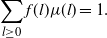 \begin{equation*} \sum_{l\geq0} f(l)\mu(l) = 1.\end{equation*}
Taking this into account, the log-likelihood of spinal-structured trees is given by
 \begin{equation*}\mathcal{L}_h^{\tiny{SST}} (\mu,f) = \sum_{\mathcal{D}(v)\lt h} \log\,\mu(\#\mathcal{C}(v)) + \sum_{v\in\mathcal{S},\,\mathcal{D}(v) \lt h} \log\,f(\#\mathcal{C}(v)).\end{equation*}
For any birth distribution
 $\mu$
, any biased distribution
 $\nu$
can be written as (1.2) with a suitable choice of f (except of course distributions
 $\nu$
such that, for some k,
 $\nu(k) \gt 0$
and
 $\mu(k)=0$
). The parametrization
 $(\mu,f)$
instead of
 $(\mu,\nu)$
makes it clearer that spinal-structured trees form a generalization of Kesten’s tree, which is obtained if and only if f is linear, considering that
 $\mu$
is subcritical. In addition, Galton–Watson trees can be seen as spinal-structured trees assuming that f is constant. Our goal in this work is to investigate the problem of estimating
 $\mu$
and f through the maximization of
 $\mathcal{L}_h^{\tiny{SST}}$
without knowledge of the types of the individuals. The main advantage of the parametrization
 $(\mu,f)$
is that, just as for Kesten’s tree, it allows us to maximize the log-likelihood with respect to
 $\mu$
without observing the types of the nodes. However, maximizing it with respect to f entails observation of the types of the nodes.
1.2. Motivation
The motivation for this paper is twofold: first, it provides a step forward in the theoretical understanding of type identification in multi-type Galton–Watson trees (MGWs); second, it offers preliminary theoretical foundations for statistically testing whether or not population data have been conditioned to survive. These two points are detailed below.
Spinal-structured trees can be seen as particular instances of two more general models. If the special individuals are interpreted as immigrants, the underlying population process is a Galton–Watson model with immigration given by
 $\nu$
. And more generally, like every Galton–Watson process with immigration, it can also be seen as a particular case of MGWs. The problem of the estimation of birth distributions in MGWs has been heavily studied, for example in [Reference Carvalho5], [Reference Cloez, Daufresne, Kerioui and Fontez6], [Reference Khaįrullin11], and [Reference Maaouia and Touati13], and references therein, but in all these works the types of the individuals are assumed to be known. A small number of works, e.g. [Reference González, Martín, Martínez and Mota9], [Reference Qi, Wang and Sun15], and [Reference Staneva and Stoimenova16], have investigated this problem with unobserved types, but none of these provide theoretical results: they only investigate numerical aspects. Using the special case of spinal-structured trees, this paper aims to demonstrate the theoretical difficulties involved in type estimation and propose a statistical strategy for dealing with them. In particular, we shall show that we are able to estimate the underlying parameters when population growth is not too large compared with the dissimilarity of the two birth distributions. This phenomenon is likely to hold true for more complicated problems.
When estimating the parameters of an observed population using a stochastic model, the latter must first be accurately chosen. To the best of our knowledge, even in the simple framework of Galton–Watson models, there is no method in the literature for rigorously determining from the data whether or not the population has been conditioned to survive. However, as mentioned above, estimating the parameters under the wrong model introduces significant biases that can lead to wrong conclusions about the population. Spinal-structured trees generalize both Galton–Watson trees (f is constant, not investigated hereafter) and Galton–Watson trees conditioned to survive (
 $f\propto\text{Id}$
). By estimating f, and even better by testing the shape of f, we can conclude which model to apply. The results of this paper will allow us to make progress in this direction (see in particular Section 7.2).
1.3. Aim of the paper
The present paper is dedicated to the development and study of an estimation method for the unknown parameters
 $\mu$
and f, as well as the unknown type of the nodes, from the observation
 $T_h$
of one spinal-structured tree until generation h. The estimation algorithm that we derive below is based on the maximization of
 $\mathcal{L}_h^{\tiny{SST}}$
with the major difficulty that types are unobserved. Once the calculations are done, it can be succinctly described as follows.
-
(i) Naive estimation of
$\mu$
:
\begin{equation*}\widehat{\mu}_h(i) = \dfrac{1}{\#T_{h}}\sum_{v\in T_h}\mathbb{1}_{\mathcal{C}(v)=i} .\end{equation*}
-
(ii) Estimation of the spine, i.e. the set of special nodes:
where
\begin{equation*} \widehat{\mathcal{S}}_{h}=\mathrm{arg\,max}_{\mathbf{s}\in\mathfrak{S}_{h}}d_{\textit{KL}}(\overline{\mathbf{s}},\mathcal{B}\widehat{\mu}_{h}),\end{equation*}
$\mathfrak{S}_{h}$
denotes the set of spine candidates (branches still alive at generation h),
$\overline{\mathbf{s}}$
is the empirical distribution of the number of children along the spine candidate
$\mathbf{s}$
,
$\mathcal{B}\widehat{\mu}_{h}(i)\propto i\,\widehat{\mu}_{h}(i)$
, and
$d_{\textit{KL}}(p,q)$
denotes the Kullback–Leibler divergence between distributions p and q.
-
(iii) Unbiased estimation of
$\mu$
(without estimated special nodes
$\widehat{\mathcal{S}}_{h}$
):
\begin{equation*}\widehat{\mu}_{h}^\star(i)=\dfrac{1}{\#T_{h}-h}\sum_{v\in T_h\setminus\widehat{\mathcal{S}}_{h}}\mathbb{1}_{\mathcal{C}(v)=i}.\end{equation*}
-
(iv) Estimation of f:
\begin{equation*}\widehat{f}_{h}(i)=\dfrac{1}{\widehat{\mu}_{h}^\star(i)h}\sum_{v\in\widehat{\mathcal{S}}_{h}}\mathbb{1}_{\mathcal{C}(v)=i}.\end{equation*}





Even in such a structured instance of MGWs, the convergence of these estimates is far from easy to establish. In Theorem 3.2 we state that if the distribution of surviving normal nodes is not too close to the special birth distribution
 $\nu$
compared to the exponential growth-rate of the tree, then
 $\widehat{\mu}^\star_h$
and
 $\widehat{f}_h$
almost surely converge towards
 $\mu$
and f. In addition, the recovered part of the spine is almost surely of order h when h goes to infinity. We insist on the fact that these two results are true for any growth regime of the tree (subcritical
 $m(\mu) \lt 1$
, critical
 $m(\mu)=1$
, or supercritical
 $m(\mu)\gt 1$
). Nevertheless, the reason behind these convergence results is not the same in the subcritical regime (where almost all of the spine can be recovered in an algorithmic fashion) and in the critical and supercritical regimes (where the number of spine candidates explodes). The theoretical convergence properties related to the asymptotics of the estimators
 $\widehat{\mu}^\star_h$
,
 $\widehat{f}_h$
, and
 $\widehat{\mathcal{S}}_h$
are shown under the following main conditions, which are essential to the proofs of convergence.
-
• The maximum number of children in the tree is
$N\geq1$
, i.e.
$\mu\in\mathcal{M}$
, where
$\mathcal{M}$
denotes the set of probability distributions on
$\{0,\dots,N\}$
. By construction (1.2),
$\nu$
also belongs to
$\mathcal{M}$
. -
•
$f(0)=0$
so that
$\nu(0)=0$
, that is, the tree admits an infinite spine of special nodes.


For the sake of readability and conciseness of the proofs, we also assume the following conditions.
-
• The support of
$\mu$
is
$\{0,\dots,N\}$
. -
•
$f(k) \gt 0$
for any
$k \gt 0$
, which implies that the support of
$\nu$
is
$\{1,\dots,N\}$
.


The article is organized as follows. Section 2 describes how some parts of the spine can be algorithmically recovered in a deterministic fashion. Section 3 is devoted to our estimation procedure and theoretical results:
-
• Section 3.1 for the preliminary estimation of
$\mu$
; -
• Section 3.2 for the identification of a candidate for the spine, named the Ugly Duckling;
-
• Section 3.3 for the final estimation of
$\mu$
and the estimation of f; -
• Section 3.4 for the statement of our main result, Theorem 3.2.


The proof of Theorem 3.2 in the subcritical case can be found in Section 4. The proof in the supercritical case involves large deviation-type estimates, for which we need information on the rate function. The rate function is studied in Section 5 and the information needed is stated in Theorem 5.1. We finally consider the proof in the critical and supercritical cases in Section 6. The final Section 7 is devoted to numerical illustrations of the results (Section 7.1) and an application to asymptotic tests for populations conditioned on surviving (Section 7.2). Appendix A concerns the proof of some intermediate lemmas.
2. Algorithmic identification of the spine
Here we propose an algorithm to (at least partially) identify the spine of a spinal-structured tree T observed until generation h. A node v of T is called observed if
 $\mathcal{D}(v) \lt h$
. It means that the number of children of v can be considered as part of the data available to reconstruct the spine of T (even if the depth of these children is h). The tree restricted to the observed nodes is denoted by
 $T_h$
.
We will also need the notion of observed height of a subtree T[v] of T. If v is a node of T, T[v] denotes the tree rooted at v and composed of v and all its descendants in T. In the literature on trees, the height
 $\mathcal{H}(T[v])$
of a subtree T[v] is the length of the longest path from its root v to its leaves. In the context of this work, T is only observed until generation h, and thus the height of T[v] can be unknown since the leaves of T[v] can be inaccessible. For this reason, we define the observed height of T[v] as
 \begin{equation*} \mathcal{H}_o(T[v]) = \min( \mathcal{H}(T[v]),\quad l-\mathcal{D}(v)),\end{equation*}
where l is the length of the minimal path from v to unobserved nodes. It should be noted that
 $\mathcal{H}_o$
implicitly depends on h. Either
 $l=+\infty$
, if v has no unobserved descendant, or
 $l = h-\mathcal{D}(v)$
. In addition, v has no unobserved descendant if and only if
 $\mathcal{H}(T[v]) + \mathcal{D}(v) \lt h$
.
The following result makes it possible to partially identify the spine.
Proposition 2.1. Let T be a spinal-structured tree observed until generation h and let v be an observed node of T.
-
• If
$\mathcal{H}_o(T[v])+\mathcal{D}(v) \lt h$
, then v is normal. -
• If v is special, the children of v are observed, and
then c is special.
\begin{equation*}\exists!\,c\in\mathcal{C}(v)\ {such\ that}\ \mathcal{H}_o(T[c])+\mathcal{D}(c)\geq h ,\end{equation*}


Proof. The proof relies on the fact that special nodes have an infinite number of descendants. First, if v is such that
 $\mathcal{H}_o(T[v])+\mathcal{D}(v) \lt h$
, it means that its subtree has become extinct before generation h and thus v is normal. Second, if v is special, exactly one of its children is special. All the subtrees rooted at the children of v that become extinct are composed of normal nodes. Consequently, if only one subtree among its children has not become extinct before generation h, it is necessarily special.
It should be noticed that if an observed node is not covered by the two previous conditions, it can be either special or normal. Indeed, if the
 $c_k$
are the children of a special node v that do not become extinct before generation h, only one of them is special, while the others are normal. In fact, only the distribution of the subtrees rooted at the
 $c_k$
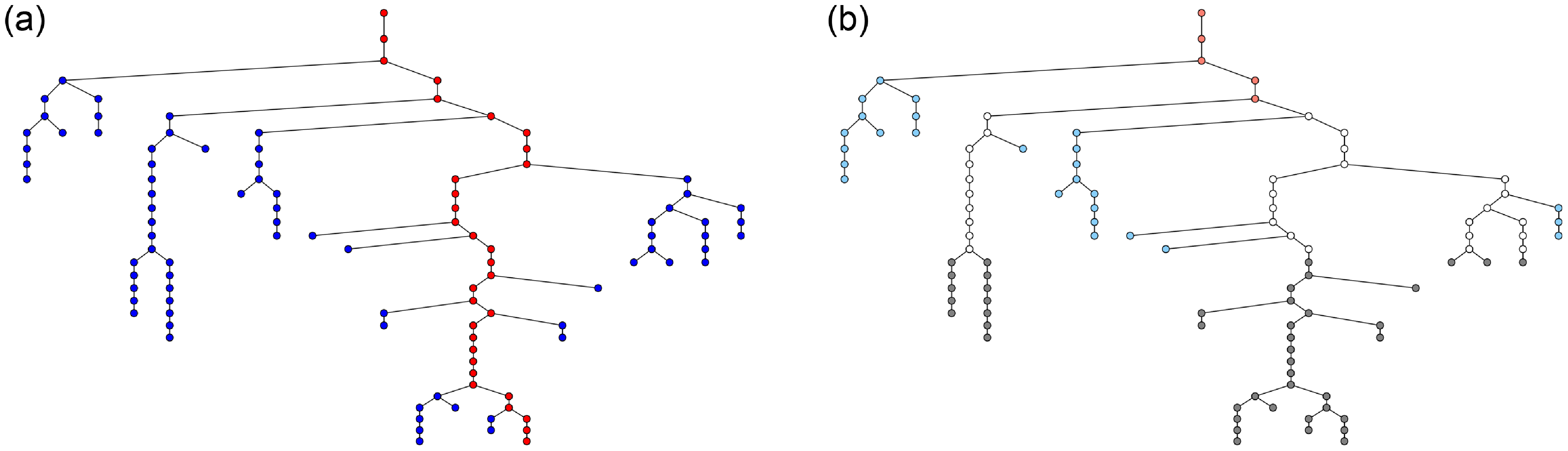
can be used to differentiate them. An application of Proposition 2.1 is presented in Figure 1.
(a) A spinal-structured tree simulated until generation 30 with normal nodes in blue and special nodes in red. We assume that it is observed until generation
 $h=15$
and in (b) we identify the type of the nodes using Proposition 2.1 with the following color code: light blue for identified normal nodes, light red for identified special nodes, gray for unobserved nodes, and white for unidentified types.
If a node v at depth
 $\mathcal{D}(v) = h-1$
has been identified as special, i.e. if v is the only node with children at depth
 $h-1$
, it means that the spine has been algorithmically reconstructed, and is formed by v and all its ancestors. Otherwise, if the type of two or more nodes at depth
 $h-1$
has not been identified, each of them is part of a possible spine. More formally, the set of possible spines
 $\mathfrak{S}_h$
is made of all the branches from the root to v whenever
 $\mathcal{D}(v) = h-1$
and the type of v has not been identified as normal. With this notation, if
 $\#\mathfrak{S}_h=1$
, then the spine has been fully reconstructed. In all cases,
 $\bigcap_{\mathbf{s}\in\mathfrak{S}_h} \mathbf{s}$
is exactly the set of nodes identified as special, while the complement
 $\bigcup_{\mathbf{s}\in\mathfrak{S}_h}\mathbf{s}\setminus \bigcap_{\mathbf{s}\in\mathfrak{S}_h}\mathbf{s}$
is composed of all the nodes that cannot be identified in an algorithmic way.
Spine candidates can be indexed by their first unobserved node. Given a node v in T, the sequence of ancestors of v is denoted by
 $\mathcal{A}(v)$
,
 \begin{equation}\mathcal{A}(v) = \bigl(\mathcal{P}^h(v) , \mathcal{P}^{h-1}(v), \dots , \mathcal{P}(v) \bigr),\end{equation}
where
 $\mathcal{P}(v)$
is the parent of v in T and recursively
 $\mathcal{P}^h(v) = \mathcal{P}(\mathcal{P}^{h-1}(v))$
. If
 $\mathcal{D}(v)=h$
, then
 $\mathcal{A}(v)$
is an element of
 $\mathfrak{S}_h$
. Throughout the paper, when there is no ambiguity, we identify
 $\mathcal{A}(v)$
with the sequence of numbers of children along
 $\mathcal{A}(v)$
, i.e.
 $(\#\mathcal{C}(u)\colon u\in\mathcal{A}(v))$
.
3. Ugly Duckling
In this section we aim to develop an estimation method for the unknown parameters
 $\mu$
and f as well as the spine
 $\mathcal{S}$
of a spinal-structured tree observed until generation h. The algorithm presented below takes advantage of the specific behavior of spinal-structured trees. We also present our main result of convergence that holds for any growth regime of the normal population, i.e. whatever the value of
 $m(\mu)$
.
3.1. Estimation of
$\mu$

As remarked in the Introduction, maximizing
 $\mathcal{L}_h^{\tiny{SST}}$
with respect to
 $\mu$
does not require us to observe the type of the nodes. Consequently, as f is unknown, we can still construct a first estimate of
 $\mu$
as
 \begin{equation*} \widehat{\mu}_h=\mathrm{arg\,max}_{\mu\in\mathcal{M}}\mathcal{L}_h^{\tiny{SST}} (\mu,f).\end{equation*}
Standard calculus shows that
 \begin{equation}\widehat{\mu}_h = \Biggl( \dfrac{1}{\#T_{h}}\sum_{v\in T_h}\mathbb{1}_{\mathcal{C}(v)=i} \Biggr)_{i\in\{0,\dots,N\}} .\end{equation}
We can notice that the optimum in f of
 $\mathcal{L}_h^{\tiny{SST}}$
depends on the unknown spine
 $\mathcal{S}$
, and is thus of no use at this stage.
3.2. Selection of the spine
In
 $\mathfrak{S}_h$
, the spine
 $\mathcal{S}$
is the unique element whose component-wise distribution is
 $\nu$
defined from (1.2). In that sense, finding
 $\mathcal{S}$
is a sample selection problem, where, however, the distribution at stake
 $\nu$
is unknown. Our approach consists in estimating the spine by the sample that differs the most from the expected behavior of a sample made of normal nodes.
However, it should be observed that the
 $\mathfrak{S}_{h}$
consist of surviving lineages. Thus
 $\mu$
is not the component-wise distribution of the samples of normal nodes in
 $\mathfrak{S}_{h}$
, and, as a consequence, is not the right distribution for comparison. Identifying the law of
 $\mathbf{s}\in\mathfrak{S}_{h}$
can be done thanks to the so-called many-to-one formula presented in the following theorem (see [Reference Lyons, Pemantle and Peres12]).
Theorem 3.1.
Let G be a Galton–Watson tree with birth distribution
 $\mu$
and let h be an integer. Then, for any bounded measurable function
 $\varphi\colon \mathbb{R}^{h}\to\mathbb{R}$
, we have
 \begin{equation}\mathbb{E}\Biggl[\sum_{\{u\in G\colon \mathcal{D}(u)=h\}}\varphi (\mathcal{A}(u))\Biggr] = m(\mu)^{h}\,\mathbb{E}[\varphi(X_{0},\ldots,X_{h-1})],\end{equation}
where
 $\mathcal{A}(u)$
is defined in (2.1) and
 $X_{1},\ldots,X_{h-1}$
is an independent and identically distributed (i.i.d.) family of random variables with common distribution
 $\mathcal{B}\mu$
, where the operator
 $\mathcal{B}$
is defined, for any
 $p\in\mathcal{M}$
, by
 \begin{equation}\mathcal{B}p(i)=\dfrac{ip_{i}}{m(p)} \quad {for\ all}\ i\in\{1,\ldots,N\}.\end{equation}
With this new information in hand, we can now define the estimate of the spine as the Ugly Duckling in
 $\mathfrak{S}_{h}$
,
 \begin{equation} \widehat{\mathcal{S}}_{h}=\mathrm{arg\,max}_{\mathbf{s}\in\mathfrak{S}_{h}}d_{\textit{KL}}(\overline{\mathbf{s}},\mathcal{B}\widehat{\mu}_{h}),\end{equation}
where
 $\overline{X}$
denotes the empirical measure associated to the vector X and
 $d_{\textit{KL}}(p,q)$
denotes the Kullback–Leibler divergence between distributions p and q. In this formula, we compare
 $\overline{\mathbf{s}}$
to
 $\mathcal{B}\widehat{\mu}_{h}$
, with
 $\widehat{\mu}_{h}$
given by (3.1), because the true distribution
 $\mu$
is obviously unknown.
Remark 3.1. Another approach would have consisted in selecting the spine as the most likely sample under
 $\nu$
, which is unknown but can be estimated from an estimate of
 $\mu$
(e.g.
 $\widehat{\mu}_{h}$
defined in (3.1)) and an estimate of f. However, as explained in Section 3.1, the optimum of
 $\mathcal{L}_h^{\tiny{SST}}$
in f depends on the spine. As a consequence, this approach would have resulted in an iterative algorithm where f is estimated from the spine, and conversely the spine from f, likely highly dependent on the initial value.
3.3. Correction of
$\mu$
and estimation of f

We can remark that the estimate (3.1) of
 $\mu$
is the empirical distribution of the numbers of children in the tree. However, the tree is made of h special nodes that do not follow
 $\mu$
, which biases the estimation. Now we know how to estimate the spine, i.e. the set of special nodes in the tree, we can take this into account and correct the estimator of
 $\mu$
as
 \begin{equation}\widehat{\mu}_{h}^\star(i)=\dfrac{1}{\#T_{h}-h}\sum_{v\in T_h\setminus\widehat{\mathcal{S}}_{h}}\mathbb{1}_{\mathcal{C}(v)=i} \quad \text{for all $ i\in\{0,\ldots,N$}\}.\end{equation}
Then we can estimate f by maximizing (under the constraint
 $\sum_{i=0}^N f(i)\widehat{\mu}_{h}^\star(i)=1$
)
 $\mathcal{L}_h^{\tiny{SST}}$
, where the unknown spine
 $\mathcal{S}$
has been replaced by
 $\widehat{\mathcal{S}}_h$
, which results in
 \begin{equation} \widehat{f}_{h}(i)=\dfrac{1}{\widehat{\mu}_{h}^\star(i)h}\sum_{v\in\widehat{\mathcal{S}}_{h}}\mathbb{1}_{\mathcal{C}(v)=i} \quad \text{for all $ i\in\{0,\ldots,N$}\}. \end{equation}
It should be noted that, by construction, no node of the spine estimate has no child, which implies
 $\widehat{f}_{h}(0)=0$
.
3.4. Theoretical results
The purpose of this section is to study the behavior of the Ugly Duckling method for large observation windows, i.e.
 $h\to\infty$
. The main difficulty arising in our problem is to recover a substantial part of the spine. Depending on the growth-rate of the population, this question takes different forms. Indeed, the number of spine candidates
 $\#\mathfrak{S}_{h}$
is highly dependent on the growth-rate
 $m(\mu)$
of the normal population in the tree.
First, in the subcritical case
 $m(\mu) \lt 1$
, the trees of normal individuals grafted onto the spine tends to become extinct. In other words, the set of spines
 $\mathfrak{S}_{h}$
is essentially reduced to
 $\mathcal{S}$
or at least to small perturbations of
 $\mathcal{S}$
. Thus a macroscopic part of the spine can be directly identified without further difficulty following the algorithm of Section 2. The only point that needs clarification is that if the unidentified part of the spine is not large enough to perturb the estimation, then we would not be able to guarantee that our estimators are convergent.
In the critical and supercritical cases, identifying the spine becomes substantially harder as the set
 $\mathfrak{S}_{h}$
may have a large size and contain potentially long lineages of non-special individuals. In particular, if the number of possible spines is large, one may observe that the empirical distribution of the number of children along some lineages
 $\mathbf{s}\in\mathfrak{S}_{h}$
may experience large deviations from its distribution, so that
 \begin{equation*}d_{\textit{KL}}(\overline{\mathbf{s}},\mathcal{B}\mu)\gg d_{\textit{KL}}(\overline{\mathcal{S}},\mathcal{B}\mu).\end{equation*}
In such a situation, one would not be able to distinguish which of
 $\mathbf{s}$
or
 $\mathcal{S}$
is the spine.
It follows that our ability to identify the spine relies on a dissimilarity/population-growth trade-off.
-
• On the one hand, if the growth-rate of the population is small, the number of possible spines is small and none of the normal spines greatly deviate from its expected distribution. Thus we can identify the sample with law
$\nu$
even if laws
$\mathcal{B}\mu$
and
$\nu$
are similar (but without being too close). -
• On the other hand, if the growth-rate is large (i.e.
$m(\mu)\gg1$
), then one may expect large deviation samples. In such a situation, we would not be able to recover the spine unless distributions
$\mathcal{B}\mu$
and
$\nu$
are very different.


One good way to measure the dissimilarity between two distributions p and q in our context is given by the following divergence:
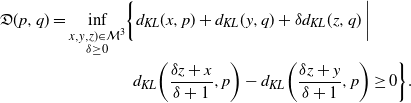 \begin{align}\mathfrak{D}(p,q)& = \inf_{\begin{subarray} (x,y,z)\in\mathcal{M}^{3}\\\quad\delta\geq0\end{subarray}} \biggl\{d_{\textit{KL}}(x,p) + d_{\textit{KL}}(y,q) + \delta d_{\textit{KL}}(z,q)\biggm| \notag \\&\quad\phantom{\inf_{\begin{subarray} (x,y,z)\in\mathcal{M}^{3}\\\quad\delta\geq0\end{subarray}}\biggl\{ }d_{\textit{KL}}\biggl(\dfrac{\delta z+x}{\delta+1},p\biggr) - d_{\textit{KL}}\biggl(\dfrac{\delta z+y}{\delta+1},p\biggr) \geq 0\biggr\}.\end{align}
This idea is summarized in the following theorem, where our convergence criterion relies on a comparison between
 $\log(m(\mu))$
and
 $\mathfrak{D}(\mathcal{B}\mu,\nu)$
.
Theorem 3.2.
If
 $\log(m(\mu))-\mathfrak{D}(\mathcal{B}\mu,\nu) \lt 0$
, then the following convergences hold almost surely:
 \begin{equation*}\widehat{\mu}_{h}^\star\xrightarrow[h\to\infty]{}\mu\end{equation*}
and
 \begin{equation*}\widehat{f}_{h} \xrightarrow[h\to\infty]{}f.\end{equation*}
In addition, an order h of the spine is recovered, that is,
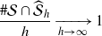 \begin{equation*}\dfrac{\#\mathcal{S}\cap\widehat{\mathcal{S}}_{h}}{h}\xrightarrow[h\to\infty]{}1\end{equation*}
almost surely.
4. Proof of Theorem 3.2 in the subcritical case
In subcritical cases, note that the criteria of Theorem 3.2 are always satisfied. In addition, it is important to note that the first step of our estimation procedure is in this case a dummy step, as it has (essentially) no use in the following steps. If
 $m(\mu) \lt 1$
, our estimation works, as for large h we can automatically identify an order h of the special individuals as the lineages of the normal ones tend to become extinct. Thus the main point to check in the proof of the subcritical case is that enough spine is directly identifiable. We directly give the proof of Theorem 3.2 in this case.
Proof of Theorem
3.2, subcritical case
 $m(\mu) \lt 1$
. The key point is that normal Galton–Watson trees induced by special individuals are very unlikely to reach a large height. As their number is finite at each generation, very few of them reach height h. In particular, they would be rather recent subtrees.
Let
 $K_{h}$
denote the length of spine that can be algorithmically identified (using the procedure presented in Proposition 2.1) when the spinal-structured tree is observed up to height h. Now, recalling that the spinal-structured tree T can be constructed by grafting an i.i.d. family of Galton–Watson trees
 $(G_{i,j})_{i,j\geq1}$
onto the spine,
 $K_{h}$
is given by
 \begin{equation*}K_{h}=\sup \{1\leq n \leq h \mid \mathcal{H}(G_{i,j})\lt h-i \ \forall\, i\in\{1,\ldots,n\},\ \forall\, j\in\{1,\ldots,S_{i}-1\} \},\end{equation*}
where
 $S_{1},\ldots,S_{h}$
denote the numbers of special children of the individuals of the spine. Thus
 \begin{align*}\mathbb{P}(K_{h}\geq n) =\mathbb{P}\Biggl(\bigcap_{i=1}^{n}\bigcap_{j=1}^{S_{i}-1}\{\mathcal{H}(G_{i,j}) \lt h-i\}\Biggr)=\prod_{i=1}^{n}\mathbb{E}\Bigl[p^{S_{i}-1}_{h-i}\Bigr],\end{align*}
where
 $p_{l}$
denotes the probability that a tree of type
 $G_{i,j}$
becomes extinct before reaching height l. We then have
 \begin{equation*}\mathbb{P}(K_{h}\geq n)\geq \prod_{i=1}^{n}p_{h-i}^{\mathbb{E}[S_{i}-1]}=\Biggl(\prod_{i=1}^{n}p_{h-i}\Biggr)^{m(\nu)-1} ,\end{equation*}
by Jensen’s inequality. Fixing some
 $\varepsilon \gt 0$
, we thus have
 \begin{equation*}\mathbb{P}\biggl(1-\dfrac{K_{h}}{h} \gt \varepsilon\biggr)=1-\mathbb{P}(K_{h}\geq \lfloor(1-\varepsilon)h\rfloor)\leq 1-\Biggl(\prod_{i=1}^{\lfloor(1-\varepsilon)h\rfloor}p_{h-i}\Biggr)^{m(\nu)-1} .\end{equation*}
In the subcritical case, it is known [Reference Athreya and Ney2] that
 \begin{equation*}p_{l}\geq1- \gamma^{l}\end{equation*}
for some real number
 $\gamma\in(0,1)$
. Hence
 \begin{equation*}\mathbb{P}\biggl(1-\dfrac{K_{h}}{h} \gt \varepsilon\biggr)\leq 1-\Biggl(\prod_{i=1}^{\lfloor(1-\varepsilon)h\rfloor}(1-\gamma^{h-i})\Biggr)^{m(\nu)-1}\leq1-(1-\gamma^{\varepsilon h})^{(m(\nu)-1)\lfloor(1-\varepsilon)h\rfloor}.\end{equation*}
It is then easily checked that
 \begin{equation*}\sum_{h\geq 1}\bigl(1-(1-\gamma^{\varepsilon h})^{(m(\nu)-1)\lfloor(1-\varepsilon)h\rfloor}\bigr) \lt \infty\end{equation*}
which, via the Borel–Cantelli lemma, entails the almost sure convergence of
 ${{K_{h}}/{h}}$
toward 1. Now, as we almost surely have
 $K_{h}\leq \#\widehat{\mathcal{S}}_{h}\cap\mathcal{S}$
, the convergence of
 $\widehat{\mu}_{h}$
and
 $\widehat{\mu}_{h}^\star$
closely follows the proof of Proposition 6.1 below, while the convergence of
 $\widehat{f}_{h}$
can be easily deduced from the Law of Large Numbers.
5. On the rate function of large deviations in sample selection
In Lemma 6.2 below, we show a large deviation-type estimate for the probability that the empirical distribution of some branch of the spinal-structured tree is closer to
 $\nu$
than that of the true spine (in Kullback–Leibler divergence). The purpose of this section is to study the rate function of this estimate, and it is a preliminary to the proof of Theorem 3.2 in the critical and supercritical cases. Throughout this section, we choose some distribution p and q in
 $\mathcal{M}$
such that
 $p\neq q$
. Our goal is to study the following parametric optimization problem referenced as problem (P
α,ε
):
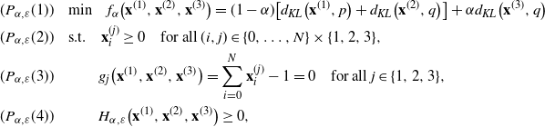 \begin{align*} & (P_{\alpha,\varepsilon}(1)) \quad \mathrm{min} \quad f_{\alpha}\bigl(\mathbf{x}^{(1)},\mathbf{x}^{(2)},\mathbf{x}^{(3)}\bigr) = (1-\alpha)\bigl[d_{\textit{KL}}\bigl(\mathbf{x}^{(1)},p\bigr)+d_{\textit{KL}}\bigl(\mathbf{x}^{(2)},q\bigr)\bigr]+\alpha d_{\textit{KL}}\bigl(\mathbf{x}^{(3)},q\bigr) \\ & (P_{\alpha,\varepsilon} (2)) \quad \text{s.t.} \quad \mathbf{x}^{(j)}_{i} \geq 0\quad\text{for all}\ (i,j)\in\{0,\ldots,N\}\times \{1,2,3\}, \\ & (P_{\alpha,\varepsilon} (3)) \qquad\quad g_{j}\bigl(\mathbf{x}^{(1)},\mathbf{x}^{(2)},\mathbf{x}^{(3)}\bigr)=\sum_{i=0}^{N}\mathbf{x}_{i}^{(j)}-1=0\quad\text{for all}\ j\in\{1,2,3\},\\ & (P_{\alpha,\varepsilon} (4)) \qquad\quad H_{\alpha,\varepsilon}\bigl(\mathbf{x}^{(1)},\mathbf{x}^{(2)},\mathbf{x}^{(3)}\bigr)\geq0, \end{align*}
where
 \begin{equation*}H_{\alpha,\varepsilon}\bigl(\mathbf{x}^{(1)},\mathbf{x}^{(2)},\mathbf{x}^{(3)}\bigr)=d_{\textit{KL}}\bigl((1-\alpha)\mathbf{x}^{(1)}+\alpha\mathbf{x}^{(3)},p\bigr)-d_{\textit{KL}}\bigl((1-\alpha)\mathbf{x}^{(2)}+\alpha\mathbf{x}^{(3)},p\bigr)+\varepsilon.\end{equation*}
The value function associated to problem (p
α,ε
) is denoted
 $V\colon [0,1]^{2}\ni(\alpha,\varepsilon)\mapsto V(\alpha,\varepsilon)\in\mathbb{R}_{+}$
and is given by
 \begin{equation}V(\alpha,\varepsilon)=\inf_{(x,y,z)\in\mathcal{M}^{3}}\{(1-\alpha)(d_{\textit{KL}}(x,p)+d_{\textit{KL}}(y,q))+\alpha d_{\textit{KL}}(z,q) \mid H_{\alpha,\varepsilon}(x,y,z) \geq 0\}.\end{equation}
In the particular situation where
 $\varepsilon=0$
, the value function associated to problem (p
α,ε
) is denoted
 $v\colon [0,1]\ni\alpha\mapsto v(\alpha)\in\mathbb{R}_{+}$
. Our goal is to show the following theorem.
Theorem 5.1.
The value function V is continuous. In addition, for any
 $\rho \in(0,1)$
, there exists
 $\varepsilon^{\ast} \gt 0$
such that
 \begin{equation*}V(\alpha,\varepsilon)\geq v(\alpha)-\rho \quad {for\ all}\ \alpha\in[0,1],\ \varepsilon\in[0,\varepsilon^{\ast}],\end{equation*}
and
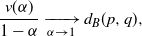 \begin{equation*}\dfrac{v(\alpha)}{1-\alpha}\xrightarrow[\alpha \to 1]{}d_{B}(p,q),\end{equation*}
where
 $d_{B}$
is the Bhattacharyya divergence defined by
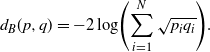 \begin{equation}d_{B}(p,q)=-2\log\Biggl(\sum_{i=1}^{N}\sqrt{p_{i}q_{i}}\Biggr).\end{equation}
To show this result, we begin by defining the parameter-dependent Lagrangian associated with problem (p α,ε ) by
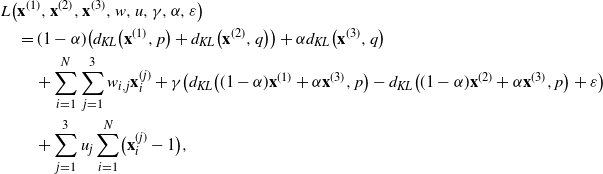 \begin{align*}& L\bigl(\mathbf{x}^{(1)},\mathbf{x}^{(2)},\mathbf{x}^{(3)},w,u,\gamma,\alpha,\varepsilon\bigr)\\&\quad = (1-\alpha)\bigl(d_{\textit{KL}}\bigl(\mathbf{x}^{(1)},p\bigr)+d_{\textit{KL}}\bigl(\mathbf{x}^{(2)},q\bigr)\bigr)+\alpha d_{\textit{KL}}\bigl(\mathbf{x}^{(3)},q\bigr)\\&\quad\quad + \sum_{i=1}^{N}\sum_{j=1}^{3}w_{i,j}\mathbf{x}^{(j)}_{i}+\gamma\bigl( d_{\textit{KL}}\bigl((1-\alpha)\mathbf{x}^{(1)}+\alpha \mathbf{x}^{(3)},p\bigr)-d_{\textit{KL}}\bigl((1-\alpha)\mathbf{x}^{(2)}+\alpha \mathbf{x}^{(3)},p\bigr)+\varepsilon\bigr) \\&\quad\quad + \sum_{j=1}^{3}u_{j}\sum_{i=1}^{N}\bigl(\mathbf{x}^{(j)}_{i}-1\bigr),\end{align*}
where
 $\gamma,u_{1}$
,
 $u_{2}$
,
 $u_{3}$
,
 $(w_{i,j})_{1\leq i\leq N,1\leq j \leq 3}$
are the Lagrange multipliers. Thus the first-order optimality conditions are given by
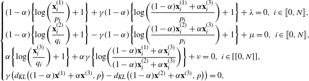 \begin{align} \begin{cases}(1-\alpha)\biggl\{\log\biggl(\dfrac{\mathbf{x}^{(1)}_{i}}{p_{i}}\biggr)+1\biggr\}+\gamma(1-\alpha)\biggl\{\log\biggl(\dfrac{(1-\alpha) \mathbf{x}^{(1)}_{i}+\alpha \mathbf{x}^{(3)}_{i}}{p_{i}}\biggr)+1\biggr\}+\lambda=0,\ i \in [[ 0,N]] , \\[5pt] (1-\alpha)\biggl\{\log\biggl(\dfrac{\mathbf{x}^{(2)}_{i}}{q_{i}}\biggr)+1\biggr\}-\gamma(1-\alpha)\biggl\{\log\biggl(\dfrac{(1-\alpha) \mathbf{x}^{(2)}_{i}+\alpha\mathbf{x}^{(3)}_{i}}{p_{i}}\biggr)+1\biggr\}+\mu=0,\ i \in[[ 0,N]] ,\\[5pt] \alpha\biggl\{\log\biggl(\dfrac{\mathbf{x}^{(3)}_{i}}{q_{i}}\biggr)+1\biggr\}+\alpha\gamma\biggl\{\log\biggl(\dfrac{(1-\alpha) \mathbf{x}^{(1)}_{i}+\alpha\mathbf{x}^{(3)}_{i}}{(1-\alpha) \mathbf{x}^{(2)}_{i}+\alpha\mathbf{x}^{(3)}_{i}}\biggr)\biggr\}+\nu=0,\ i \in[[0,N]],\\[5pt] \gamma\bigl(d_{\textit{KL}}\bigl((1-\alpha)\mathbf{x}^{(1)}+\alpha \mathbf{x}^{(3)},p\bigr)-d_{\textit{KL}}\bigl((1-\alpha)\mathbf{x}^{(2)}+\alpha \mathbf{x}^{(3)},p\bigr)\bigr)=0, \end{cases}\end{align}
where
 $\lambda$
,
 $\mu$
,
 $\nu$
are the Lagrange multipliers associated with the constraints (p
α,ε
(3)) (corresponding to u in the definition of the Lagrangian).
Let us point out that these optimality conditions do not hold for feasible points such that
 $\mathbf{x}^{(i)}_{j}=0$
for some i and j, because our problem is not smooth at these points. It only holds for feasible points in the interior of
 $\mathbb{R}_{+}^{3(N+1)}$
. In Lemma 5.1, we show that there is no optimal solution in the boundary of
 $\mathbb{R}_{+}^{3(N+1)}$
that justifies the use of conditions (5.3). The set of Lagrange multipliers associated with a feasible point (x, y, z) is denoted
 $\mathbf{L}(x,y,z)$
(and is a subset of
 $\mathbb{R}_{-}^{3(N+1)}\times\mathbb{R}^{3}\times \mathbb{R}_{-}$
). In particular, let us emphasize that due to the inequality constraint (p
α,ε
(4)), we require
 $\gamma\leq 0$
. We let
 $\mathbf{S}(\alpha,\varepsilon)$
denote the set of solutions of the above problem for given parameters
 $(\alpha,\varepsilon)$
and let
 $\mathbf{F}(\alpha,\varepsilon)$
be the set of feasible points. In the particular case where
 $\varepsilon=0$
, we use the notation
 $\mathbf{S}(\alpha)$
and
 $\mathbf{F}(\alpha)$
for
 $\mathbf{S}(\alpha,0)$
and
 $\mathbf{F}(\alpha,0)$
respectively. Our first goal is to show that for any
 $\bigl(\mathbf{x}^{(1)},\mathbf{x}^{(2)},\mathbf{x}^{(3)}\bigr)\in \mathbf{S}(\alpha,\varepsilon)$
, we have
 $\mathbf{x}^{(j)}_{i} \gt 0$
for all i,j. This is the point of the following lemma.
Lemma 5.1.
Consider the set
 $\mathbf{S}(\alpha,\varepsilon)$
of solutions of problem (p
α,ε
). Then, for
 $\varepsilon$
small enough and any
 $\alpha\in(0,1)$
, we have
 \begin{equation*}\mathbf{S}(\alpha,\varepsilon)\cap \partial\mathbb{R}_{+}^{3(N+1)}=\emptyset.\end{equation*}
Proof. The proof has been deferred to Appendix A.1.
Remark 5.1. In the cases where
 $\varepsilon=0$
, note that one can easily check using the first-order optimally conditions that the inequality constraint (p α,ε(4)) is always saturated. Thus, in the following, we will always assume that
 $\gamma \lt 0$
.
Proof of Theorem 5.1.
Step 1: Solving (P0,0) i.e.
 $\alpha=\varepsilon=0$
. In this case the first-order optimality conditions (5.3) become
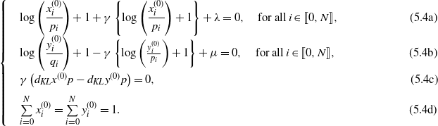 \begin{equation*}\begin{cases}&\log\left(\cfrac{x^{(0)}_{i}}{p_{i}}\right)+1+\gamma\left\{\log\left(\cfrac{ x^{(0)}_{i}}{p_{i}}\right)+1\right\}+\lambda=0,\quad \text{for all}\,i \in [[ 0,N]], \qquad\qquad\qquad(5.4\text{a})\\[6pt] &\log\left(\cfrac{y^{(0)}_{i}}{q_{i}}\right)+1-\gamma\left\{\log\left(\frac{y^{(0)}_{i}}{p_{i}}\right)+1\right\}+\mu=0,\quad \text{for all}\,i \in[[ 0,N]], \qquad\qquad\qquad\;(5.4\text{b})\\[6pt] &\gamma\left(d_{KL}{x^{(0)}}{p}-d_{KL}{y^{(0)}}{p}\right)=0,\qquad\qquad\qquad\qquad\qquad\qquad\qquad\qquad\qquad\qquad\quad\ \ \, (5.4\text{c})\\[6pt] &\sum\limits_{i=0}^{N} x^{(0)}_{i}=\sum\limits_{i=0}^{N} y^{(0)}_{i}=1.\qquad\qquad\qquad\qquad\qquad\qquad\qquad\qquad\qquad\qquad\qquad\qquad\ \ \; (5.4\text{d})\end{cases}\end{equation*}
If we assume that
 $\gamma\neq -1$
, then (5.4a), (5.4c), and (5.4d) lead to
 \begin{equation*}x^{(0)}_{i}=y^{(0)}_{i}=p_{i}\quad \text{for all}\ i \in [[ 0,N]],\end{equation*}
which is not compatible with (5.4d) unless
 $p=q$
. In addition,
 $\gamma=0$
leads to
 $x^{(0)}=p$
and
 $y^{(0)}=q$
, which is easily checked to be not feasible. Thus we have
 $\gamma= -1$
, and (5.4b) then gives
 \begin{equation*}y^{(0)}_{i}\,{\mathrm{e}}^{\mu/2}=\sqrt{p_{i}q_{i}}\quad \text{for all}\ i\in [[ 0,N]] ,\end{equation*}
which, using (5.4d), gives
 \begin{equation*}y^{(0)}_{i}=\dfrac{\sqrt{p_{i}q_{i}}}{\sum_{l=0}^{N}\sqrt{p_{l}q_{l}}}\quad \text{for all}\ i\in [[ 0,N]].\end{equation*}
It follows from (5.4c) that
 $\bigl(x^{(0)},y^{(0)},z^{(0)}\bigr)$
, with
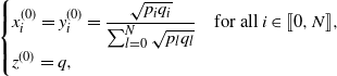 \begin{equation*}\begin{cases}x^{(0)}_{i}=y^{(0)}_{i}=\dfrac{\sqrt{p_{i}q_{i}}}{\sum_{l=0}^{N}\sqrt{p_{l}q_{l}}}\quad \text{for all}\ i \in [[ 0,N]],\\z^{(0)}=q,\end{cases}\end{equation*}
is a feasible optimal solution of problem (P 0,0). In particular,
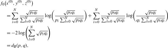 \begin{align*} &f_{0}\bigl(x^{(0)},y^{(0)},z^{(0)}\bigr)\\ &\quad=\sum_{i=0}^{N}\dfrac{\sqrt{p_{i}q_{i}}}{\sum_{l=0}^{N}\sqrt{p_{i}q_{i}}}\log\biggl(\dfrac{\sqrt{p_{i}q_{i}}}{p_{i}\sum_{l=0}^{N}\sqrt{p_{i}q_{i}} }\biggr)+\sum_{i=0}^{N}\dfrac{\sqrt{p_{i}q_{i}}}{\sum_{l=0}^{N}\sqrt{p_{i}q_{i}}}\log\biggl(\dfrac{\sqrt{p_{i}q_{i}}}{q_{i}\sum_{l=0}^{N}\sqrt{p_{i}q_{i}} }\biggr)\\ &\quad =-2\log\Biggl(\sum_{l=0}^{N}\sqrt{p_{i}q_{i}} \Biggr)\\ &\quad =d_{B}(p,q),\end{align*}
where
 $d_{B} (\cdot,\cdot)$
is the Bhattacharyya divergence defined in (5.2).
Step 2: Continuity of the value function. The goal of this step is to show that the full value function V is continuous. To do so, we apply Theorem 2.1 in conjunction with Theorem 2.8 of [Reference Fiacco and Ishizuka8]. In view of these theorems, the only point that needs clarification is that
 \begin{equation*}\overline{\{(x,y,z)\in \mathcal{M}^{3} \mid H_{\alpha,\varepsilon}(x,y,z) \gt 0\}}=\{(x,y,z)\in \mathcal{M}^{3} \mid H_{\alpha,\varepsilon}(x,y,z)\geq0\}.\end{equation*}
To do so, it suffices to show that for any
 $(a,b,c)\in \mathcal{M}^{3}$
such that
 $H_{\alpha,\varepsilon}(a,b,c)=0$
and any
 $\delta \gt 0$
, there exists an element
 $(\tilde{a},\tilde{b},\tilde{c})\in \mathcal{M}^{3}$
such that
 $H_{\alpha,\varepsilon}(\tilde{a},\tilde{b},\tilde{c}) \gt 0$
with
 \begin{equation*}\|(a,b,c)-(\tilde{a},\tilde{b},\tilde{c})\|_1 \lt \delta.\end{equation*}
As the proof closely follows the ideas of the proof of Lemma 5.1, we do not write down the details. Thus V is continuous. The first statement of Theorem 5.1 now follows from the compactness of [0,1].
Step 3: Limits of
 ${{v(\alpha)}/{(1-\alpha)}}$
as
 $\alpha\to1$
. For any
 $\alpha \in[0,1)$
, it is easily seen that
 \begin{align*} \dfrac{v(\alpha)}{1-\alpha} & = \inf_{(x,y,z)\in \mathcal{M}^{3}} \biggl\{d_{\textit{KL}}(x,p)+d_{\textit{KL}}(y,q)+\dfrac{\alpha\,d_{\textit{KL}}(z,q)}{1-\alpha}\biggm| \\ &\quad \phantom{\inf_{(x,y,z)\in \mathcal{M}^{3}} \biggl\{} d_{\textit{KL}}\biggl(x+\dfrac{\alpha}{1-\alpha}z,p\biggr)-d_{\textit{KL}}\biggl(y+\dfrac{\alpha}{1-\alpha}z,p\biggr)\geq 0 \biggr\}.\end{align*}
This is equivalent to studying the behavior of
 \begin{equation}\mathcal{V}(\delta)=\inf_{(x,y,z)\in \mathcal{M}^{3}} \{d_{\textit{KL}}(x,p)+d_{\textit{KL}}(y,q)+\delta d_{\textit{KL}}(z,q)\mid d_{\textit{KL}}(x+\delta z,p)-d_{\textit{KL}}(y+\delta z,p)\geq 0 \},\end{equation}
as
 $\delta$
goes to infinity. So, let
 $(\delta_n)_{n\geq 1}$
be some sequence of real numbers such that
 $\delta_n\xrightarrow[n\to \infty]{}\infty$
, and set
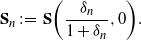 \begin{equation*}\mathbf{S}_n \,:\!=\, \mathbf{S}\biggl(\dfrac{\delta_n}{1+\delta_n},0\biggr).\end{equation*}
Now, for all
 $n\geq 1$
, choose
 $(x^{(n)},y^{(n)},z^{(n)})\in \mathbf{S}_n$
. As
 $\cup_{n\geq 1}\mathbf{S}_{n}\subset \mathcal{M}$
is relatively compact, we may assume, extracting a subsequence if needed, that
 $(x^{(n)},y^{(n)},z^{(n)})$
converges to some element
 $(x^{\ast},y^{\ast},z^{\ast})\in \mathcal{M}^{3}$
. Now assume that
 \begin{equation*}\lim_{n\to \infty}\|z^{(n)}-q\|_{1} \gt 0.\end{equation*}
However, this would imply that
 $\liminf_{n\to\infty}d_{\textit{KL}}(z^{(n)},q) \gt 0$
, and thus that
 \begin{equation*}\liminf_{n\to \infty}\{ d_{\textit{KL}}(x^{(n)},p)+d_{\textit{KL}}(y^{(n)},q)+\delta_{n}d_{\textit{KL}}(z^{(n)},q)\}\geq \liminf_{n\to \infty}\delta_{n}d_{\textit{KL}}(z^{(n)},q)=\infty,\end{equation*}
but this is impossible, since, according to Step 1,
 $\mathcal{V}(\delta)\leq d_{B}(p,q)$
(because the solution given in Step 1 is always feasible). It follows that
 \begin{equation*}\lim_{n\to \infty}\|z^{(n)}-q\|_{1}=0\end{equation*}
and
 $z^{\ast}=q$
. Now, for fixed
 $n\geq 1$
, the first-order optimality conditions of problem (5.5) take the form
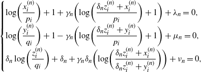 \begin{align} \begin{cases}\log\biggl(\dfrac{x^{(n)}_{i}}{p_{i}} \biggr)+1+\gamma_n\biggl(\log\biggl(\dfrac{\delta_nz^{(n)}_{i}+x^{(n)}_{i}}{p_{i}} \biggr)+1\biggr) +\lambda_n=0,\\[6pt] \log\biggl(\dfrac{y^{(n)}_{i}}{q_{i}} \biggr)+1-\gamma_n\biggl(\log\biggl(\dfrac{\delta_nz^{(n)}_{i}+y^{(n)}_{i}}{p_{i}} \biggr)+1\biggr) +\mu_n=0,\\[6pt] \delta_n\log\biggl(\dfrac{z^{(n)}_{i}}{q_{i}} \biggr)+\delta_n+\gamma_n\delta_n\biggl(\log\biggl(\dfrac{\delta_nz^{(n)}_{i}+x^{(n)}_{i}}{\delta_nz^{(n)}_{i}+y^{(n)}_{i}} \biggr)\biggr) +\nu_n=0,\end{cases}\end{align}
for some Lagrange multipliers
 $(\lambda_{n},\mu_{n},\nu_{n},\gamma_{n})\in\mathbf{L}(x^{(n)},y^{(n)},z^{(n)})$
.
We now show that the sequence
 $\gamma_{n}$
must be bounded. For this, let us assume that
 $\gamma_{n}$
is unbounded. So, extracting a subsequence if needed, we may assume that
 \begin{equation*} \gamma_{n}\xrightarrow[n\to\infty]{}-\infty. \end{equation*}
The second equation of (5.6) implies that, for all i,
 \begin{equation*}\dfrac{y_{i}^{(n)}p_{i}}{q_{i}}=p_{i}\biggl(\dfrac{\delta_{n}z^{(n)}_{i}+y_{i}^{(n)}}{p_{i}}\biggr)^{\gamma_{n}}\exp({-}1+\gamma_{n}-\mu_{n}).\end{equation*}
Summing over i and using Jensen’s inequality (since
 $\gamma_{n} \lt 0$
), we obtain
 \begin{equation*}\sum_{i=1}^{N}\dfrac{y_{i}^{(n)}p_{i}}{q_{i}}=\sum_{i=1}^{N}p_{i}\biggl(\dfrac{\delta_{n}z^{(n)}_{i}+x_{i}^{(n)}}{p_{i}}\biggr)^{\gamma_{n}}\exp({-}1+\gamma_{n}-\mu_{n})\geq(1+\delta_{n})^{\gamma_{n}}\exp({-}1+\gamma_{n}-\mu_{n}).\end{equation*}
Thus
 \begin{equation*}\log\Biggl(\sum_{i=1}^{N}\dfrac{y_{i}^{(n)}p_{i}}{q_{i}}\Biggr)-\gamma_{n}\log(1+\delta_{n})+1-\gamma_{n}+\mu_{n}\geq 0.\end{equation*}
Now equations (5.6) also give, for all
 $1\leq i\leq N$
,
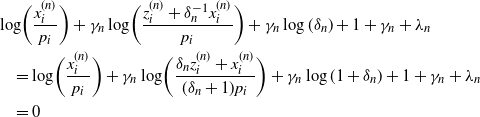 \begin{align}& \log\biggl(\dfrac{x^{(n)}_{i}}{p_{i}} \biggr)+\gamma_n\log\biggl(\dfrac{z^{(n)}_{i}+\delta_{n}^{-1}x^{(n)}_{i}}{p_{i}} \biggr)+\gamma_n\log(\delta_n) +1+\gamma_{n}+\lambda_n \nonumber\\ &\quad = \log\biggl(\dfrac{x^{(n)}_{i}}{p_{i}} \biggr)+\gamma_n\log\biggl(\dfrac{\delta_{n}z^{(n)}_{i}+x^{(n)}_{i}}{(\delta_{n}+1)p_{i}} \biggr)+\gamma_n\log(1+\delta_n) +1+\gamma_{n}+\lambda_n \notag \\ &\quad =0 \end{align}
and
 \begin{equation*} \log\biggl(\dfrac{y^{(n)}_{i}}{q_{i}} \biggr)-\gamma_n\log\biggl(\dfrac{\delta_{n}z^{(n)}_{i}+y^{(n)}_{i}}{(\delta_{n}+1)p_{i}} \biggr)-\gamma_n\log(1+\delta_n) +1+\gamma_{n}+\mu_n=0.\end{equation*}
Hence, for n large enough, we have
 \begin{equation*}\log\biggl(\dfrac{y^{(n)}_{i}}{q_{i}} \biggr)-\gamma_n\log\biggl(\dfrac{\delta_{n}z^{(n)}_{i}+y^{(n)}_{i}}{(\delta_{n}+1)p_{i}} \biggr)-\log\Biggl(\sum_{i=1}^{N}\dfrac{y_{i}^{(n)}p_{i}}{q_{i}}\Biggr)\leq 0.\end{equation*}
In particular, this implies that
 $y^{\ast}_{i}=0$
for all i such that
 $q_{i} \gt p_{i}$
. Similarly to (5.7), we get
 \begin{equation*}\log\biggl(\dfrac{x^{(n)}_{i}}{p_{i}} \biggr)+\gamma_n\log\biggl(\dfrac{\delta_{n}z^{(n)}_{i}+x^{(n)}_{i}}{(\delta_{n}+1)p_{i}} \biggr)\leq 0,\end{equation*}
and
 $x^{\ast}_{i}=0$
for all i such that
 $p_{i} \gt q_{i}$
. Now a direct computation gives
 \begin{equation*}d_{\textit{KL}}(x^{\ast},p)+d_{\textit{KL}}(y^{\ast},q)\geq -\log\Biggl(\sum_{j\in J}p_{i}\Biggr)-\log\Biggl(\sum_{i\in I}q_{i}\Biggr),\end{equation*}
with
 $I=\{i\in\{1,\ldots,N\}\mid q_{i}\leq p_{i}\}$
and
 $J=\{i\in\{1,\ldots,N\}\mid p_{i}\leq q_{i}\}$
. However,
 \begin{equation*}\Biggl(\sum_{i\in J }p_{i}\Biggr)\Biggl(\sum_{i\in I }q_{i}\Biggr)\leq\Biggl( \sum_{i\in J }\sqrt{p_{i}q_{i}}\Biggr)\Biggl( \sum_{i\in I }\sqrt{p_{i}q_{i}}\Biggr) \lt \Biggl( \sum_{i=1 }^{N}\sqrt{p_{i}q_{i}}\Biggr)^{2}.\end{equation*}
Thus
 \begin{equation*} -\log\Biggl(\sum_{j\in J}p_{i}\Biggr)-\log\Biggl(\sum_{i\in I}q_{i}\Biggr) \gt d_{B}(p,q).\end{equation*}
But, as the solution of Step 1 is always an admissible solution, this is absurd since it would imply that, for n large enough,
 $(x^{(n)},y^{(n)},z^{(n)})$
is not optimal. From the preceding, we conclude that
 $\gamma_{n}$
is bounded. Thus, again extracting a subsequence if needed, we can suppose that there exists some
 $\gamma_{\infty}\leq 0$
such that
 \begin{equation*}\gamma_{n}\xrightarrow[n\to\infty]{} \gamma_{\infty}.\end{equation*}
In addition, (5.7) implies that the sequence
 $(\gamma_n\log(\delta_n) +\lambda_n)_{n\geq 1}$
is bounded as well (because there must be at least one i such that
 $\lim_{n\to\infty }x^{(n)}_{i} \gt 0$
), which we may also assume to be convergent. From these and (5.7), it follows that
 \begin{equation}x_{i}^{(n)}=p_{i}^{1+\gamma_{n}}q_{i}^{-\gamma_{n}}\,{\mathrm{e}}^{c_{n}+\gamma_{n}{\mathrm{O}} (\delta_{n}^{-1})}=\dfrac{p_{i}^{1+\gamma_{\infty}}q_{i}^{-\gamma_{\infty}}}{\sum_{j=1}^{N}p_{j}^{1+\gamma_{\infty}}q_{j}^{-\gamma_{\infty}}}+{\mathrm{o}} (1) \quad \text{for all $ 1\leq i\leq n$,}\end{equation}
and similarly, we have
 \begin{equation}y_{i}^{(n)}=p_{i}^{-\gamma_{n}}q_{i}^{1-\gamma_{n}}\,{\mathrm{e}}^{\tilde{c}_{n}+\gamma_{n}{\mathrm{O}} (\delta_{n}^{-1})}=\dfrac{p_{i}^{-\gamma_{\infty}}q_{i}^{1+\gamma_{\infty}}}{\sum_{j=1}^{N}p_{j}^{-\gamma_{\infty}}q_{j}^{1+\gamma_{\infty}}}+{\mathrm{o}} (1)\quad \text{for all $ 1\leq i\leq n$,}\end{equation}
where
 $(c_{n})_{n\geq 1}$
and
 $(\tilde{c_{n}})_{n\geq 1}$
are some convergent sequences. Denoting
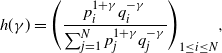 \begin{equation*}h(\gamma)=\Biggl(\dfrac{p_{i}^{1+\gamma}q_{i}^{-\gamma}}{\sum_{j=1}^{N}p_{j}^{1+\gamma}q_{j}^{-\gamma}}\Biggr)_{1\leq i\leq N},\end{equation*}
and setting
 $K(x)=d_{\textit{KL}}(x,p)$
for any
 $x\in\mathcal{M}$
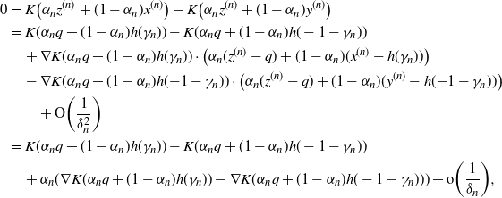
, it follows that (see Remark 5.1)
 \begin{align*}0&= K\bigl(\alpha_{n} z^{(n)}+(1-\alpha_{n})x^{(n)}\bigr)-K\bigl(\alpha_{n} z^{(n)}+(1-\alpha_{n})y^{(n)}\bigr)\\&= K(\alpha_{n}q+(1-\alpha_{n})h(\gamma_{n}))-K(\alpha_{n}q+(1-\alpha_{n})h(-1-\gamma_{n}))\\&\quad + \nabla K(\alpha_{n}q+(1-\alpha_{n})h(\gamma_{n}))\cdot\bigl(\alpha_{n}(z^{(n)}-q)+(1-\alpha_{n})(x^{(n)}-h(\gamma_{n}))\bigr)\\&\quad - \nabla K(\alpha_{n}q+(1-\alpha_{n})h({-}1-\gamma_{n}))\cdot\bigl(\alpha_{n}(z^{(n)}-q)+(1-\alpha_{n})(y^{(n)}-h({-}1-\gamma_{n}))\bigr)\\&\quad\quad +{\mathrm{O}}\biggl(\dfrac{1}{\delta_{n}^{2}}\biggr)\\&= K(\alpha_{n}q+(1-\alpha_{n})h(\gamma_{n}))-K(\alpha_{n}q+(1-\alpha_{n})h(-1-\gamma_{n}))\\&\quad + \alpha_{n}(\nabla K(\alpha_{n}q+(1-\alpha_{n})h(\gamma_{n}))-\nabla K(\alpha_{n}q+(1-\alpha_{n})h(-1-\gamma_{n})))+{\mathrm{o}}\biggl(\dfrac{1}{\delta_{n}}\biggr),\end{align*}
but since
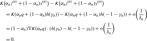
 $\nabla K$
exists and is continuous in a neighborhood of q, we get
 \begin{align*}& K\bigl(\alpha_{n} z^{(n)}+(1-\alpha_{n})x^{(n)}\bigr)-K\bigl(\alpha_{n} z^{(n)}+(1-\alpha_{n})y^{(n)}\bigr)\\&\quad = K(\alpha_{n}q+(1-\alpha_{n})h(\gamma_{n}))-K(\alpha_{n}q+(1-\alpha_{n})h(-1-\gamma_{n}))+{\mathrm{o}}\biggl(\dfrac{1}{\delta_{n}}\biggr)\\&\quad = (1-\alpha_{n})\nabla K(\alpha_{n}q)\cdot(h(\gamma_{n})-h(-1-\gamma_{n}))+{\mathrm{o}}\biggl(\dfrac{1}{\delta_{n}}\biggr)\\&\quad = 0.\end{align*}
Finally, as
 $1-\alpha_{n}\sim {{1}/{\delta_{n}}}$
, it follows that
 \begin{equation*}\nabla K(q)\cdot(h(\gamma_{\infty})-h(1-\gamma_{\infty}))=0.\end{equation*}
Now, since
 $\nabla K(q)=(\log(q_{i}/p_{i})+1)_{1\leq i\leq N}$
, we have
 \begin{equation}\sum_{i=1}^{N}\log\biggl(\dfrac{q_{i}}{p_{i}}\biggr)(h_{i}(\gamma_{\infty})-h_{i}(-1-\gamma_{\infty}))=0.\end{equation}
Since
 $p_{i}^{1+\gamma}q_{i}^{-\gamma}=(p_{i}/q_{i})^{-\gamma-1/2}(p_{i}q_{i})^{1/2}$
, (5.10) can be written as
 \begin{equation}F({-}\gamma_{\infty}-1/2)=F(\gamma_{\infty}+1/2),\end{equation}
where
 $F(\gamma)=F_{1}(\gamma)/F_{0}(\gamma)$
with, for any
 $k\in\mathbb{N}$
,
 \begin{equation*}F_{k}(\gamma) \,:\!=\, \sum_{i=1}^{N}\log^{k}\biggl(\dfrac{q_{i}}{p_{i}}\biggr)\cdot \biggl(\dfrac{q_{i}}{p_{i}}\biggr)^{\gamma}\sqrt{p_{i}q_{i}}.\end{equation*}
Let
 $\overline{\gamma_{\infty}} \,:\!=\, -\gamma_{\infty}-1/2$
, which implies that (5.11) can be rewritten as
 $F(\overline{\gamma}_{\infty})=F(-\overline{\gamma}_{\infty})$
. We shall show that the only solution of this equation is
 $\overline{\gamma}_{\infty}=0$
. One can see that
 $F(1/2)=d_{\textit{KL}}(q,p) \gt 0$
and
 $F({-}1/2)=-d_{\textit{KL}}(p,q) \lt 0$
. Since
 $F^{\prime}_{k}=F_{k+1}$
, we obtain
 \begin{equation*}F^{\prime}=\dfrac{F_{1}^{\prime}F_{0}-F_{1}F_{0}^{\prime}}{F_{0}^{2}}=\dfrac{F_{2}F_{0}-F_{1}^{2}}{F_{0}^2} \gt 0\end{equation*}
by the Cauchy–Schwarz inequality, because
 $\log(q_{i}/p_{i})$
is not constant by
 $p\neq q$
. Thus F is a strictly increasing function, which implies that the only solution is
 $\overline{\gamma}_{\infty}=0$
. Hence
 $\gamma_{\infty}=1/2$
, which finally gives, according to (5.8) and (5.9),
 \begin{equation*}x^{\ast}_{i}=y^{\ast}_{i}=\dfrac{\sqrt{p_{i}q_{i}}}{\sum_{j=1}^{N}\sqrt{p_{j}q_{j}}}\quad \text{for all $ 1\leq i\leq N$.}\end{equation*}
From this, it follows that
 \begin{equation*}\mathcal{V}(\delta_{n})\xrightarrow[n\to\infty]{}d_{B}(p,q),\end{equation*}
which, since the sequence
 $(\delta_{n})_{n\geq 1}$
is arbitrary, implies that
 \begin{equation*}\lim_{\alpha\to 1}\dfrac{v(\alpha)}{1-\alpha}=\lim_{\delta\to\infty}\mathcal{V}(\delta)=d_{B}(p,q).\end{equation*}
This ends the proof.
6. Proof of Theorem 3.2 in the critical and supercritical cases
The purpose of this section is to prove Theorem 3.2 when
 $m(\mu)\geq1$
.
6.1. Estimation of
$\mu$

We aim to prove that
 $\widehat{\mu}_{h}$
is always convergent in these cases.
Proposition 6.1.
If
 $m(\mu)\geq1$
, then the estimators
 $\widehat{\mu}_{h}$
and
 $\widehat{\mu}_{h}^{\ast}$
, defined in (3.1) and (3.5) respectively, satisfy
 \begin{equation*}\widehat{\mu}_{h}\xrightarrow[h\to\infty]{}\mu\end{equation*}
and
 \begin{equation*}\widehat{\mu}_{h}^{\ast}\xrightarrow[h\to\infty]{}\mu\end{equation*}
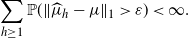
almost surely. In addition, for any
 $\varepsilon \gt 0$
we have
 \begin{equation*}\sum_{h\geq 1}\mathbb{P}(\|\widehat{\mu}_{h}-\mu\|_{1} \gt \varepsilon) \lt \infty.\end{equation*}
Note that the result of Proposition 6.1 is rather intuitive. Indeed, when the normal Galton–Watson subtrees are supercritical, the sample used in (3.1) or (3.5) is a perturbation of size h of a
 $\mu$
i.i.d. sample whose size is of order
 $m(\mu)^{h}$
. Therefore our primary concern is ensuring that this perturbation is not sufficiently large to hinder the estimation process.
Proof. Recall that the spinal-structured tree T can be decomposed as the grafting of a sequence
 $(G_{i,j})_{i,j\geq 1}$
of i.i.d. Galton–Watson trees with common birth distribution
 $\mu$
onto the spine. For each of these trees, let us write
 $\overline{X}_{i,j,h}$
, for
 $i,j,h\in\mathbb{N}$
, the random vector defined by
 \begin{equation*}\overline{X}_{i,j,h}(k)=\sum_{\{v\in G_{i,j}\colon \mathcal{D}(v)\lt h\}}\mathbb{1}_{\mathcal{C}(v)=k},\quad 0\leq k \leq N.\end{equation*}
We emphasize that i corresponds to generations in the spinal-structured tree whereas j corresponds to indices of the offspring in a given generation. In addition, it is known (see e.g. [Reference Devroye7]) that the law of
 $\overline{X}_{i,j,h}$
conditional on
 $\#\{v\in G_{i,j}\colon \mathcal{D}(v)\lt h\}$
is multinomial with parameters
 $\mu$
and
 $\#\{v\in G_{i,j}\colon \mathcal{D}(v)\lt h\}$
. From this, and from the independence of the
 $G_{i,j}$
, it follows that the random variable
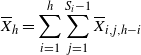
 $\overline{X}_h$
defined by
 \begin{equation*}\overline{X}_{h}=\sum_{i=1}^{h}\sum_{j=1}^{S_{i}-1}\overline{X}_{i,j,h-i}\end{equation*}
is, conditionally on
 $\#T_{h}$
, a multinomial random variable with parameters
 $\#T_{h}-h$
and
 $\mu$
independent of
 $\mathcal{S}_{h}$
. Now, letting
 $\overline{\mathcal{S}_{h}}$
denote the empirical distribution associated with
 $\mathcal{S}_{h}$
, that is,
 \begin{equation*}\overline{\mathcal{S}_{h}}(k)=\dfrac{1}{h}\sum_{i=1}^{h}\mathbb{1}_{S_{i}=k}\quad \text{for all $ k\in\{1,\ldots,N\}$,}\end{equation*}
where
 $S_{1},\ldots, S_{h}$
denote the numbers of special children of the individuals of the spine, it is easily seen that
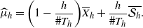 \begin{equation*}\widehat{\mu}_{h}=\biggl(1-\dfrac{h}{\#T_{h}}\biggr)\overline{X}_{h}+\dfrac{h}{\#T_{h}}\overline{\mathcal{S}_{h}}.\end{equation*}
Now, taking
 $\varepsilon \gt 0$
, Pinsker’s inequality entails that
 \begin{equation*}\mathbb{P}\bigl(\|\widehat{\mu}_{h}-\mu\|_{1} \gt \sqrt{\varepsilon/2}\bigr)\leq\mathbb{P}(d_{\textit{KL}}(\widehat{\mu}_{h},\mu) \gt \varepsilon).\end{equation*}
The convexity of the Kullback–Leibler divergence gives, with
 $\alpha_{h} \,:\!=\, {{h}/{\#T_{h}}}$
,
 \begin{align*} \mathbb{P}\bigl(\|\widehat{\mu}_{h}-\mu\|_{1} \gt \sqrt{\varepsilon/2}\bigr)&\leq\mathbb{P}\bigl((1-\alpha_{h})d_{\textit{KL}}\bigl(\overline{X}_{h},\mu\bigr)+\alpha_{h}d_{\textit{KL}}\bigl(\overline{\mathcal{S}_{h}},\mu\bigr) \gt \varepsilon\bigr)\\ &\leq \mathbb{P}\biggl((1-\alpha_{h})d_{\textit{KL}}\bigl(\overline{X}_{h},\mu\bigr)+\alpha_{h}d_{\textit{KL}}\bigl(\overline{\mathcal{S}_{h}},\mu\bigr) \gt \varepsilon,\ \alpha_{h}d_{\textit{KL}}(\nu,\mu) \lt \dfrac{\varepsilon}{2}\biggr)\\ &\quad +\mathbb{P}\biggl( \alpha_{h}d_{\textit{KL}}(\nu,\mu)\geq \dfrac{\varepsilon}{2}\biggr).\end{align*}
Next, using the method of Lemma 6.2, one can show that for any
 $\delta \gt 0$
there is a constant
 $C \gt 0$
such that
 \begin{align*}&\mathbb{P}\biggl((1-\alpha_{h})d_{\textit{KL}}\bigl(\overline{X}_{h},\mu\bigr)+\alpha_{h}d_{\textit{KL}}\bigl(\overline{\mathcal{S}_{h}},\mu\bigr) \gt \varepsilon,\ \alpha_{h}d_{\textit{KL}}(\mu,\nu) \lt \dfrac{\varepsilon}{2}\biggm| \#T_{h}\biggr)\\&\quad \leq C \exp(-\#T_{h}(\Gamma(\alpha_{h})-\delta)),\end{align*}
with
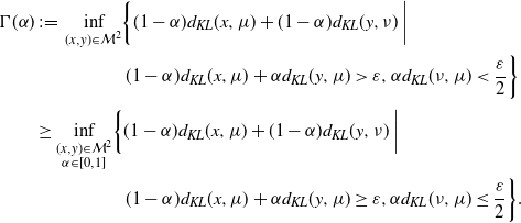 \begin{align*} \Gamma(\alpha) & \,:\!=\, \inf_{(x,y)\in \mathcal{M}^{2}} \biggl\{(1-\alpha)d_{\textit{KL}}(x,\mu)+(1-\alpha)d_{\textit{KL}}(y,\nu)\biggm| \notag \\ &\quad\ \phantom{\inf_{(x,y)\in \mathcal{M}^{2}} \biggl\{} (1-\alpha)d_{\textit{KL}}(x,\mu)+\alpha d_{\textit{KL}}(y,\mu) \gt \varepsilon,\alpha d_{\textit{KL}}(\nu,\mu) \lt \dfrac{\varepsilon}{2}\biggr\} \nonumber \\ & \geq \inf_{\substack{(x,y)\in \mathcal{M}^{2}\\ \alpha\in[0,1]}} \biggl\{(1-\alpha)d_{\textit{KL}}(x,\mu)+(1-\alpha)d_{\textit{KL}}(y,\nu)\biggm| \notag \\ &\quad\ \phantom{\inf_{\substack{(x,y)\in \mathcal{M}^{2}\\ \alpha\in[0,1]}} \biggl\{} (1-\alpha)d_{\textit{KL}}(x,\mu)+\alpha d_{\textit{KL}}(y,\mu)\geq \varepsilon,\alpha d_{\textit{KL}}(\nu,\mu)\leq\dfrac{\varepsilon}{2} \biggr\}.\end{align*}
As the feasible set of the right-hand side is obviously compact, there exists a feasible point
 $(x^{\ast},y^{\ast},\alpha^{\ast})$
such that
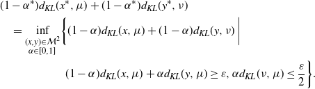 \begin{align*}& (1-\alpha^{\ast})d_{\textit{KL}}(x^{\ast},\mu)+(1-\alpha^{\ast})d_{\textit{KL}}(y^{\ast},\nu)\\ &\quad = \inf_{\substack{(x,y)\in \mathcal{M}^{2}\\\alpha\in[0,1]}} \biggl\{(1-\alpha)d_{\textit{KL}}(x,\mu)+(1-\alpha)d_{\textit{KL}}(y,\nu)\biggm|\\ &\quad\quad \phantom{\inf_{\substack{(x,y)\in \mathcal{M}^{2}\\\alpha\in[0,1]}} \biggl\{} (1-\alpha)d_{\textit{KL}}(x,\mu)+\alpha d_{\textit{KL}}(y,\mu)\geq \varepsilon,\alpha d_{\textit{KL}}(\nu,\mu)\leq\dfrac{\varepsilon}{2} \biggr\}.\end{align*}
Assume that
 $(1-\alpha^{\ast})d_{\textit{KL}}(x^{\ast},\mu)+(1-\alpha^{\ast})d_{\textit{KL}}(y^{\ast},\nu)=0$
, which readily implies that
 $x^{\ast}=\mu$
and
 $y^{\ast}=\nu$
, but it is easily seen that for any
 $\alpha\in[0,1]$
, the point
 $(\mu,\nu,\alpha)$
is not feasible. Hence there exists a constant
 $\widetilde{C} \gt 0$
independent of
 $\alpha$
such that
 \begin{equation*}\Gamma(\alpha)\geq \widetilde{C}.\end{equation*}
Choosing
 $\delta \lt \widetilde{C}$
, we get
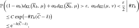 \begin{align*} &\mathbb{P}\biggl((1-\alpha_{h})d_{\textit{KL}}\bigl(\overline{X}_{h},\mu\bigr)+\alpha_{h}d_{\textit{KL}}\bigl(\overline{\mathcal{S}_{h}},\mu\bigr) \gt \varepsilon,\ \alpha_{h}d_{\textit{KL}}(\mu,\nu) \lt \dfrac{\varepsilon}{2}\biggm| \#T_{h}\biggr) \\ &\quad \leq C \exp\bigl(-\#T_{h}(\widetilde{C}-\delta)\bigr)\\&\quad \leq {\mathrm{e}}^{-h(\widetilde{C}-\delta)},\end{align*}
since
 $\#T_{h}\geq h$
. Then
 \begin{equation*}\mathbb{P}\bigl(\|\widehat{\mu}_{h}-\mu\|_{1} \gt \sqrt{\varepsilon/2}\bigr)\leq {\mathrm{e}}^{-hC}+\mathbb{P}\biggl( \alpha_{h}d_{\textit{KL}}(\mu,\nu)\geq \dfrac{\varepsilon}{2}\biggr).\end{equation*}
To ensure that the right-hand side of the previous inequality is summable for
 $h\geq 1$
, it thus remains to check that
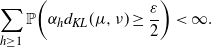 \begin{equation*}\sum_{h\geq 1}\mathbb{P}\biggl( \alpha_{h}d_{\textit{KL}}(\mu,\nu)\geq \dfrac{\varepsilon}{2}\biggr) \lt \infty.\end{equation*}
From this point we assume that the birth distribution is critical. The supercritical case is considered below. So, to treat this, we observe that the spinal-structured tree (excluding the spine) can be interpreted as a Galton–Watson tree with immigration with birth distribution
 $\mu$
and immigration
 $\tilde{\nu}$
given by
 $\tilde{\nu}_{k}=\nu_{k+1}$
for
 $k\geq 0$
. It is known (see [Reference Pakes14]) that the generating function of
 $\#T_{h}$
is given by
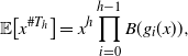 \begin{equation}\mathbb{E}\bigl[x^{\#T_{h}}\bigr]=x^{h}\prod_{i=0}^{h-1}B(g_{i}(x)),\end{equation}
where
 $B\colon [0,1]\mapsto \mathbb{R}$
is the generating function of the law
 $\tilde{\nu}$
, and
 $g_{i}$
is the generating function of the total progeny of a Galton–Watson tree with law
 $\mu$
up to generation i, that is,
 \begin{equation*}g_{i}(x)=\mathbb{E}\bigl[x^{\sum_{j=0}^{i}Z_{j}}\bigr] \quad \text{for all $ x\in[0,1]$,}\end{equation*}
where
 $(Z_{i})_{i\geq 0}$
is a standard Galton–Watson process with birth distribution
 $\mu$
. Now denote
 \begin{equation*}v_{h}=\mathbb{E}\bigl[x^{{{\#T_{h}}/{h}}}\bigr] \quad \text{for all $ h\geq 1$.}\end{equation*}
We then have (the regularity of B and
 $g_{i}$
is easily checked)
 \begin{equation*}\log(v_{h})=\log(B(g_{i}(\theta_{h})))+(\theta_{h+1}-\theta_{h})\dfrac{g^{\prime}_{i}(\eta_{h})B^{\prime}(g_{i}(\eta_{h}))}{B(g_{i}(\eta_{h}))},\end{equation*}
with
 \begin{equation}\theta_{h}=\exp\biggl(\dfrac{\log(x)}{h}\biggr)\text{ and }\eta_{h}\in(\theta_{h},\theta_{h+1})\quad\text{for all $ h\geq 1$.}\end{equation}
Hence (6.1) entails that
 \begin{equation*}\log\biggl(\dfrac{v_{h+1}}{v_{h}}\biggr)=\log(x)+(\theta_{h+1}-\theta_{h})\sum_{i=0}^{h-1}\dfrac{g^{\prime}_{i}(\eta_{h})B^{\prime}(g_{i}(\eta_{h}))}{B(g_{i}(\eta_{h}))}+\log(B(g_{h}(\theta_{h+1}))).\end{equation*}
Now, as the sequence
 $g_{i}$
is monotonically decreasing and converging to some proper generating function g (only in the critical case; see again [Reference Pakes14]), we obtain
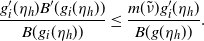 \begin{equation*}\dfrac{g^{\prime}_{i}(\eta_{h} )B^{\prime}(g_{i}(\eta_{h}))}{B(g_{i}(\eta_{h}))}\leq \dfrac{m(\tilde{\nu})g_{i}^{\prime}(\eta_{h})}{B(g(\eta_{h}))}.\end{equation*}
Now, as for
 $x\in(0,1)$
,
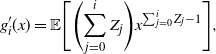 \begin{equation*}g_{i}^{\prime}(x)=\mathbb{E}\Biggl[\Biggl(\sum_{j=0}^{i}Z_{j}\Biggr)x^{\sum_{j=0}^{i}Z_{j}-1}\Biggr],\end{equation*}
we have
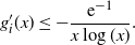 \begin{equation*}g_{i}^{\prime}(x)\leq- \dfrac{{\mathrm{e}}^{-1}}{x\log(x)}.\end{equation*}
It follows that
 \begin{align*}\limsup_{h\to\infty}\log\biggl(\dfrac{v_{h+1}}{v_{h}}\biggr)&\leq \log(x)-\limsup_{h\to\infty}\biggl((\theta_{h+1}-\theta_{h})\dfrac{m(\tilde{\nu})}{B(g(\eta_{h}))}\dfrac{h\,{\mathrm{e}}^{-1}}{\eta_{h}\log(\eta_{h})}+\log(B(g_{h}(\theta_{h+1})))\biggr)\\&= \log(x)+m(\tilde{\nu})\,{\mathrm{e}}^{-1},\end{align*}
where we used (6.2) to get
 \begin{equation*}\lim\limits_{h\to\infty}h\eta_{h}\log(\eta_{h})=\log(x).\end{equation*}
Now, as x is arbitrary, it can always be chosen such that
 $\log(x)+m(\tilde{\nu})\,{\mathrm{e}}^{-1} \lt 0$
, which, by the ratio test, implies that, for such x,
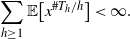 \begin{equation*}\sum_{h\geq 1}\mathbb{E}\bigl[x^{{{\#T_{h}}/{h}}}\bigr] \lt \infty.\end{equation*}
Finally, we have
 \begin{equation*}\mathbb{E}\bigl[x^{{{\#T_{h}}/{h}}}\bigr]\geq \mathbb{E}\bigl[x^{{{\#T_{h}}/{h}}}\mathbb{1}_{{{\#T_{h}}/{h}}\leq c_{\varepsilon}}\bigr]\geq x^{c_{\varepsilon}}\mathbb{P}\biggl(\dfrac{\#T_{h}}{h}\leq c_{\varepsilon}\biggr),\end{equation*}
where
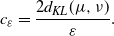 \begin{equation*}c_{\varepsilon}=\dfrac{2d_{\textit{KL}}(\mu,\nu)}{\varepsilon}.\end{equation*}
From this, it follows that
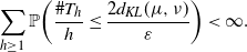 \begin{equation}\sum_{h\geq 1}\mathbb{P}\biggl(\dfrac{\#T_{h}}{h}\leq \dfrac{2d_{\textit{KL}}(\mu,\nu)}{\varepsilon}\biggr) \lt \infty.\end{equation}
We now consider the case where
 $T_{h}$
is supercritical. A possible approach is to consider a coupling between the supercritical tree
 $T_{h}$
and a critical tree
 $\widetilde{T}_{h}$
using a thinning procedure, in order to get the estimate
 \begin{equation}\mathbb{E}\bigl[x^{{{\#T_{h}}/{h}}}\bigr]\leq \mathbb{E}\bigl[x^{{{\#\widetilde{T}_{h}}/{h}}}\bigr].\end{equation}
Indeed, now assume that
 $T_{h}$
is supercritical. We consider a thinning of
 $T_{h}$
where each normal individual (and its descent) is killed independently with probability p. This induces a new tree
 $\widetilde{T}_{h}$
with new normal birth distribution
 $\widetilde{\mu}$
such that
 $m(\widetilde{\mu})=pm(\mu)$
. So taking
 $p=m(\mu)^{-1}$
implies that
 $\widetilde{T}_{h}$
is a spinal-structured tree with critical birth distribution. Hence, from the first part of the proof, we have
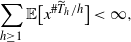 \begin{equation*}\sum_{h\geq 1}\mathbb{E}\bigl[x^{{{\#\widetilde{T}_{h}}/{h}}}\bigr] \lt \infty,\end{equation*}
for x such that
 $\log(x)+m(\tilde{\nu})\,{\mathrm{e}}^{-1} \lt 0$
. But the thinning procedure used for constructing
 $\widetilde{T}_{h}$
directly implies that
 $\#\widetilde{T}_{h}\leq \#T_{h}$
almost surely, which gives (6.4). This implies that
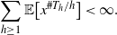 \begin{equation*}\sum_{h\geq 1}\mathbb{E}\bigl[x^{{{\#T_{h}}/{h}}}\bigr] \lt \infty.\end{equation*}
The remainder of the proof is the same as for the critical case. This ends the proof of the almost sure convergence of
 $\widehat{\mu}_{h}$
. Concerning the almost sure convergence of
 $\widehat{\mu}_{h}^{\ast}$
, first note that (6.3) implies that
 \begin{equation}\dfrac{h}{\#T_{h}}\xrightarrow[h\to\infty]{}0\end{equation}
almost surely. Now take any
 $\mathbf{s}\in\mathfrak{S}_{h}$
, where we recall that
 $\mathfrak{S}_{h}$
is the set of spine candidates defined in Section 2, and consider the estimator
 $\mu^{\mathbf{s}}_{h}$
given by
 \begin{equation*}\mu^{\mathbf{s}}_{h}(i)=\dfrac{1}{\#T_{h}-h}\sum_{v\in T_h\setminus\mathbf{s}}\mathbb{1}_{\mathcal{C}(v)=i}\quad \text{for all $ 0\leq i \leq N$.}\end{equation*}
Thus
 \begin{equation*}|\widehat{\mu}_{h}(i)-\widehat{\mu}_{h}^{\mathbf{s}}(i)|\leq \widehat{\mu}_{h}\biggl|1-\dfrac{\#T_{h}}{\#T_{h}-h}\biggr|+\dfrac{\#\mathbf{s}}{\#T_{h}-h}=\widehat{\mu}_{h}\biggl|1-\dfrac{\#T_{h}}{\#T_{h}-h}\biggr|+\dfrac{h}{\#T_{h}-h},\end{equation*}
and the result follows from (6.5) and the almost sure convergence of
 $\widehat{\mu}_{h}$
.
6.2. Spine recovery
Now, to go further in the proof of Theorem 3.2, we need to understand whether we can recover enough of the spine in order to estimate f. To do so, the idea is to show that the Ugly Duckling
 $\widehat{\mathcal{S}}_{h}$
contains a proportion of order h of special individuals. Before this result, we need some preliminary lemmas. The first one concerns Kullback–Leibler divergence.
Lemma 6.1.
Let
 $p\in\mathcal{M}$
such that
 $p_{-} \,:\!=\, \inf_{0\leq i \leq N}p_{i} \gt 0$
and
 $m(p)\geq 1$
. Then there exists
 $\varepsilon_{1} \gt 0$
such that, for any
 $q,\hat{p}\in\mathcal{M}$
, we have
 \begin{equation*}\|p-\hat{p}\|_{1} \lt \varepsilon_{1}\Longrightarrow |d_{\textit{KL}}(q,\mathcal{B}p)-d_{\textit{KL}}(q,\mathcal{B}\hat{p})|\leq C_{1}\|p-\hat{p}\|_{1},\end{equation*}
where
 $C_{1}$
depends only on p.
Proof. The proof has been deferred to Appendix A.2.
The following lemma concerns large deviations on the probability of distinguishing two samples.
Lemma 6.2.
Let p and q in
 $\mathcal{M}$
. Let R, M, and S be three independent multinomial random variables with respective parameters
 $(h-n,p)$
,
 $(h-n,q)$
, and (n,q), for some integers h and n such that
 $h \gt n$
. Then, for any
 $\delta \gt 0$
, there exists a constant
 $C \gt 0$
such that
 \begin{equation*}\mathbb{P}(d_{\textit{KL}}(M+S,p)+\varepsilon \gt d_{\textit{KL}}(R+S,p))\leq C \exp\{h(-(1-\alpha)\mathfrak{D}(p,q)+\varepsilon-\delta) \},\end{equation*}
where
 $\mathfrak{D}$
is the divergence defined in (3.7). In addition the constant C depends only on N and
 $\delta$
.
Proof. The proof has been deferred to Appendix A.3.
We can finally come to the proof of Theorem 3.2.
Proof of Theorem 3.2, critical and supercritical cases. Let us recall that, for any element
 $\mathbf{s}\in\mathfrak{S}_{h}$
,
 $\bar{\mathbf{s}}$
is defined as the random vector given by
 \begin{equation*}\bar{\mathbf{s}}_{i}=\dfrac{1}{h}\sum_{v\in\mathbf{s}}\mathbb{1}_{\mathcal{C}(v)=i}\quad \text{for all $ 0\leq i \leq N$,}\end{equation*}
that is, the empirical distribution of the numbers of children along
 $\mathbf{s}$
. In addition, for any non-negative integer
 $l\leq h$
, we let
 $\mathfrak{S}_{h}^{l}$
denote the subset of
 $\mathfrak{S}_{h}$
such that
 \begin{equation*}\mathfrak{S}_{h}^{l}=\{\mathbf{s}\in\mathfrak{S}_{h} \mid \#(\mathbf{s}\cap \mathcal{S})\leq l \}.\end{equation*}
From the definition of
 $\widehat{\mathcal{S}}_{h}$
, we have, for any non-negative integer l,
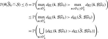 \begin{align*}\mathbb{P}(\#(\widehat{\mathcal{S}}_{h}\cap\mathcal{S} )\leq l )&= \mathbb{P}\biggl(\max_{\mathbf{s}\in\mathfrak{S}_{h}^{l}}d_{\textit{KL}}(\bar{\mathbf{s}},\mathcal{B}\widehat{\mu}_{h}) \gt \max_{\mathbf{s}\in\mathfrak{S}_{h}\setminus\mathfrak{S}_{h}^{k}}d_{\textit{KL}}(\bar{\mathbf{s}},\mathcal{B}\widehat{\mu}_{h})\biggr)\\&\leq \mathbb{P}\biggl(\max_{\mathbf{s}\in\mathfrak{S}_{h}^{l}}d_{\textit{KL}}(\bar{\mathbf{s}},\mathcal{B}\widehat{\mu}_{h}) \gt d_{\textit{KL}}(\bar{\mathcal{S}},\mathcal{B}\widehat{\mu}_{h})\biggr)\\&= \mathbb{P}\Biggl(\bigcup_{\mathbf{s}\in\mathfrak{S}_{h}^{l}}\{d_{\textit{KL}}(\bar{\mathbf{s}},\mathcal{B}\widehat{\mu}_{h}) \gt d_{\textit{KL}}(\bar{\mathcal{S}},\mathcal{B}\widehat{\mu}_{h})\}\Biggr).\end{align*}
Now let
 $\varepsilon \gt 0$
such that
 $\varepsilon \lt \varepsilon_1$
, where
 $\varepsilon_1$
is defined in Lemma 6.1. Thus, according to Lemma 6.1, we have
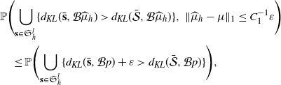 \begin{align*} &\mathbb{P}\Biggl(\bigcup_{\mathbf{s}\in \mathfrak{S}_{h}^{l}}\{d_{\textit{KL}}(\bar{\mathbf{s}},\mathcal{B}\widehat{\mu}_{h}) \gt d_{\textit{KL}}(\bar{\mathcal{S}},\mathcal{B}\widehat{\mu}_{h})\},\ \|\widehat{\mu}_{h}-\mu\|_{1}\leq C_{1}^{-1}\varepsilon\Biggr)\\ &\quad \leq \mathbb{P}\Biggl(\bigcup_{\mathbf{s}\in \mathfrak{S}_{h}^{l}}\{d_{\textit{KL}}(\bar{\mathbf{s}},\mathcal{B}p)+\varepsilon \gt d_{\textit{KL}}(\bar{\mathcal{S}},\mathcal{B}p)\}\Biggr),\end{align*}
where
 $C_{1}$
is also defined in Lemma 6.1. Hence, following the notation of (3.2), we have
 \begin{align*} \mathbb{P}(\#(\widehat{\mathcal{S}}_{h}\cap\mathcal{S} )\leq l ) & \leq \mathbb{E}\Biggl[\sum_{i=0}^{l}\sum_{j=1}^{S_i}\sum_{\{u\in G_{i,j}\colon \mathcal{D}(u)=i\}}\mathbb{1}_{d_{\textit{KL}}((1-{{i}/{h}})\overline{\mathcal{A}(u)}+{{i}/{h}}\overline{\mathcal{S}_{i}},\mathcal{B}p)+\varepsilon \gt d_{\textit{KL}}(\overline{\mathcal{S}_{h}},\mathcal{B}p)}\Biggr]\\ &\quad +\mathbb{P}\bigl(\|\widehat{\mu}_{h}-\mu\|_{1} \gt C_{1}^{-1}\varepsilon\bigr)\\ & = \mathbb{E}[S]\sum_{i=0}^{l}\mathbb{E}\Biggl[\sum_{\{u\in G\colon \mathcal{D}(u)=i\}}\mathbb{1}_{d_{\textit{KL}}({{i}/{h}}\overline{\mathcal{A}(u)}+(1-{{i}/{h}})\overline{\mathcal{S}_{i}},\mathcal{B}p)+\varepsilon \gt d_{\textit{KL}}(\overline{\mathcal{S}_{h}},\mathcal{B}p)}\Biggr]\\ &\quad +\mathbb{P}\bigl(\|\widehat{\mu}_{h}-\mu\|_{1} \gt C_{1}^{-1}\varepsilon\bigr),\end{align*}
where G is some Galton–Watson tree with birth distribution
 $\mu$
and we recall that
 $\mathcal{S}_{i}=(S_{1},\ldots,S_{i})$
are the i first elements of the spine. Now, applying the many-to-one formula (3.2), we get
 \begin{align*}& \mathbb{E}\Biggl[\sum_{\{u\in G\colon \mathcal{D}(u)=h\}}\mathbb{1}_{d_{\textit{KL}}({{i}/{h}}\overline{\mathcal{A}(u)}+(1-{{i}/{h}})\overline{\mathcal{S}_{h-i}},p)+\varepsilon \gt d_{\textit{KL}}(\bar{\mathcal{S}},p)}\Biggr]\\&\quad = m^{i}\mathbb{P}\biggl(d_{\textit{KL}}\biggl(\dfrac{i}{h}\overline{X}+\biggl(1-\dfrac{i}{h}\biggr)\overline{\mathcal{S}_{h-i}},p\biggr)+\varepsilon \gt d_{\textit{KL}}\bigl(\overline{\mathcal{S}_{h}},p\bigr)\biggr),\end{align*}
where
 $\overline{X}$
is the empirical distribution of an i.i.d. sample
 $X_1,\ldots,X_i$
with law given by
 $\mathcal{B}\mu$
independent of
 $\mathcal{S}$
.
Now let
 $\rho \gt 0$
be such that
 $\log(m(\mu))-\mathfrak{D}(\mathcal{B}\mu,\nu)+\rho \lt 0$
. Thus, according to Lemma 6.2 and Theorem 5.1, we can choose
 $\delta \gt 0$
and
 $\varepsilon$
small enough such that
 $V(\alpha,\varepsilon)\geq v(\alpha)-\rho$
and
 \begin{equation*}\mathbb{P}\bigl(\#\bigl(\widehat{\mathcal{S}}_{h}\cap \mathcal{S} \bigr)\leq l \bigr)\leq C_{\delta} \mathbb{E}[S]\sum_{i=0}^{l}m^{h-i}\exp\biggl(-h \biggl(v\biggl(\dfrac{i}{h}\biggr)-\rho\biggr)+h\delta\biggr)+\mathbb{P}\bigl(\|\widehat{\mu}_{h}-\mu\|_{1} \gt C_{1}^{-1}\varepsilon\bigr),\end{equation*}
for some constant
 $C_{\delta}$
provided by Lemma 6.2. Now let
 $\eta \gt 0$
; setting
 $\mathcal{E}_{h}=h-\#(\widehat{\mathcal{S}}_{h}\cap \mathcal{S} )$
, we have
 \begin{align*}\mathbb{P}\biggl(\dfrac{\mathcal{E}_{h}}{h} \gt \eta\biggr)&= \mathbb{P}\bigl(\#\bigl(\widehat{\mathcal{S}}_{h}\cap \mathcal{S}\bigr)\leq \lfloor(1-\delta) h\rfloor\bigr)\\&\leq C_{\delta}\mathbb{E}[S]\sum_{\alpha\in L_h}\exp(h((1-\alpha)\log(m)- v(\alpha)+\rho+\delta))+\mathbb{P}(\|\widehat{\mu}_{h}-\mu\|_{1} \gt \varepsilon),\end{align*}
with
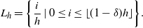 \begin{equation*}L_h=\biggl\{\frac{i}{h}\mid0\leq i\leq \lfloor (1-\delta)h\rfloor\biggr\}.\end{equation*}
One can now easily control the probability by
 \begin{equation*}\mathbb{P}\biggl(\dfrac{\mathcal{E}_{h}}{h} \gt \eta\biggr)\leq C_{\delta}\mathbb{E}[S](h+1)\exp\biggl(h\sup_{\alpha\in [0,(1-\eta)]}\bigl\{(1-\alpha)\log(m)- V(\alpha)+\rho+\delta\bigr\}\biggr).\end{equation*}
Now let us denote
 \begin{equation*}\alpha_\eta \,:\!=\, \mathrm{arg\,max}_{\alpha \in [0,(1-\eta)]}(1-\alpha)\log(m)- V(\alpha).\end{equation*}
Since
 $(1-\alpha)\log(m)- V(\alpha)\lt 0$
for all
 $\alpha\in [0,1)$
, we have
 \begin{equation*}\alpha_\eta\xrightarrow[\eta\to 0]{}1,\end{equation*}
by virtue of the continuity of V. Now, according to Theorem 5.1, we have
 \begin{equation*}(1-\alpha)\log(m)- v(\alpha)\sim_{\alpha \to 1}(1-\alpha)(\log(m)-d_{B}(p,q)).\end{equation*}
Thus, for a fixed
 $\kappa \gt 0$
and for
 $\eta$
small enough, we have
 \begin{equation*}(1-\alpha_\eta)\log(m)-v(\alpha_\eta)\leq (1-\kappa)(1-\alpha_\eta)(\log(m)-d_{B}(p,q)),\end{equation*}
which gives
 \begin{equation*}\mathbb{P}\biggl(\dfrac{\mathcal{E}_{h}}{h} \gt \eta\biggr)\leq C_{\delta}\mathbb{E}[S](h+1)\exp(h\{(1+\kappa)(1-\alpha_\eta)(\log(m)-d_{B}(p,q))+\rho+\delta\}).\end{equation*}
Thus, for
 $\rho$
and
 $\delta$
small enough, we find that
 $\mathbb{P}({{\mathcal{E}}/{h}} \gt \eta)$
converges to zero exponentially fast, which entails that
 \begin{equation*}\dfrac{\mathcal{E}_{h}}{h}\xrightarrow[h\to\infty]{}0\end{equation*}
almost surely, and ends the proof.
7. Simulation study
The numerical results presented in this section were obtained using the Python library treex [Reference Azaïs, Cerutti, Gemmerlé and Ingels3] dedicated to tree simulation and analysis.
7.1. Consistency of estimators
This part is devoted to the illustration of the consistency result stated in Theorem 3.2 through numerical simulations. For each of three normal birth distributions
 $\mu$
(subcritical, critical, and supercritical), we have simulated 50 spinal-structured trees until generation
 $h_{\max}+1$
, with
 $h_{\max}=125$
. The birth distribution of special nodes
 $\nu$
is obtained from
 $\mu$
and f using (1.2), where the only condition imposed on f (in the critical and supercritical regimes) was that the convergence criterion
 $\mathcal{K}(\mu,\nu) = \log\,m(\mu)-\mathfrak{D}(\mathcal{B}\mu,\nu)$
is negative. The values of the parameters selected for this simulation study are presented in Table 1.
Values of the parameters
 $\mu$
and f selected for the simulation of the spinal-structured trees in the subcritical, critical, and supercritical regimes, as well as the associated convergence criterion
 $\mathcal{K}(\mu,\nu) = \log\,m(\mu)-\mathfrak{D}(\mathcal{B}\mu,\nu)$
.
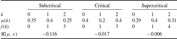
For each of these trees, we have estimated the unknown model parameters for observation windows h between 5 and
 $h_{\max}$
with a step of 5. The normal birth distribution is estimated twice: by the (biased) maximum likelihood estimator
 $\widehat{\mu}_{h}$
given in (3.1) and by the corrected estimator
 $\widehat{\mu}_{h}^\star$
defined in (3.5). The transform function f is estimated by
 $\widehat{f}_{h}$
defined in (3.6). Finally, the special birth distribution
 $\nu$
is estimated by
 \begin{equation*}\widehat{\nu}_h(k) \propto \widehat{f}_{h}(k)\widehat{\mu}_{h}^\star(k)\quad \text{for all $ 0\leq k\leq N$.}\end{equation*}
For these four numerical parameters, we have computed the error in the
 $L^1$
-norm (since f is identifiable only up to a multiplicative constant, both f and
 $\widehat{f}_{h}$
were normalized so that their sum is 1 as before). The spine is estimated by the Ugly Duckling
 $\widehat{\mathcal{S}}_{h}$
defined in (3.4). In this case, the estimation error is given by the proportion of special nodes not recovered by
 $\widehat{\mathcal{S}}_{h}$
.
The average errors computed for each of the five estimators from varying observation windows h are presented for the three growth regimes in Figure 2. First of all, note that the five average errors tend to vanish when h increases (even if it is with different shapes) for any growth regime (the convergence criterion is checked in the three examples). This illustrates the consistency of the estimators stated in Theorem 3.2. However, additional pieces of information can be obtained from these simulations.
-
• It can be remarked that the correction of
$\widehat{\mu}_{h}$
is useful only in the subcritical regime. In the two other regimes, one can indeed observe that the errors related to
$\widehat{\mu}_{h}$
and
$\widehat{\mu}_{h}^\star$
are almost superimposed. This is due to the fact that, in these growth regimes, the number of normal nodes is sufficiently large (compared to the number of special nodes) so that the bias of the maximum likelihood estimator vanishes. -
• The estimators of f and
$\nu$
are clearly less accurate than
$\widehat{\mu}_{h}^\star$
, in particular in the critical and supercritical regimes. A first but likely negligible reason is that
$\widehat{f}_{h}$
is computed from
$\widehat{\mu}_{h}^\star$
, which should only add an error to the one associated with the latter. Furthermore, the number of special nodes (used to estimate
$\widehat{f}_{h}$
) is smaller than the number of normal nodes (used to estimate
$\widehat{\mu}_{h}^\star$
). -
• The estimator of the spine seems to converge, but slowly compared to the other estimates. However, we emphasize that, when h increases, the number of unknown node types increases as well, contrary to
$\mu$
, f, and
$\nu$
, for which the dimension is fixed. It is thus expected to observe a slower convergence rate.


Average error as a function of the maximum height observed in the estimation of the unknown parameters (orange and red,
 $\mu$
; blue, f; light blue,
 $\nu$
; green,
 $\mathcal{S}$
) of a spinal-structured tree in the three growth regimes: (a) subcritical, (b) critical, (c) supercritical. Parameter values can be read in Table 1.
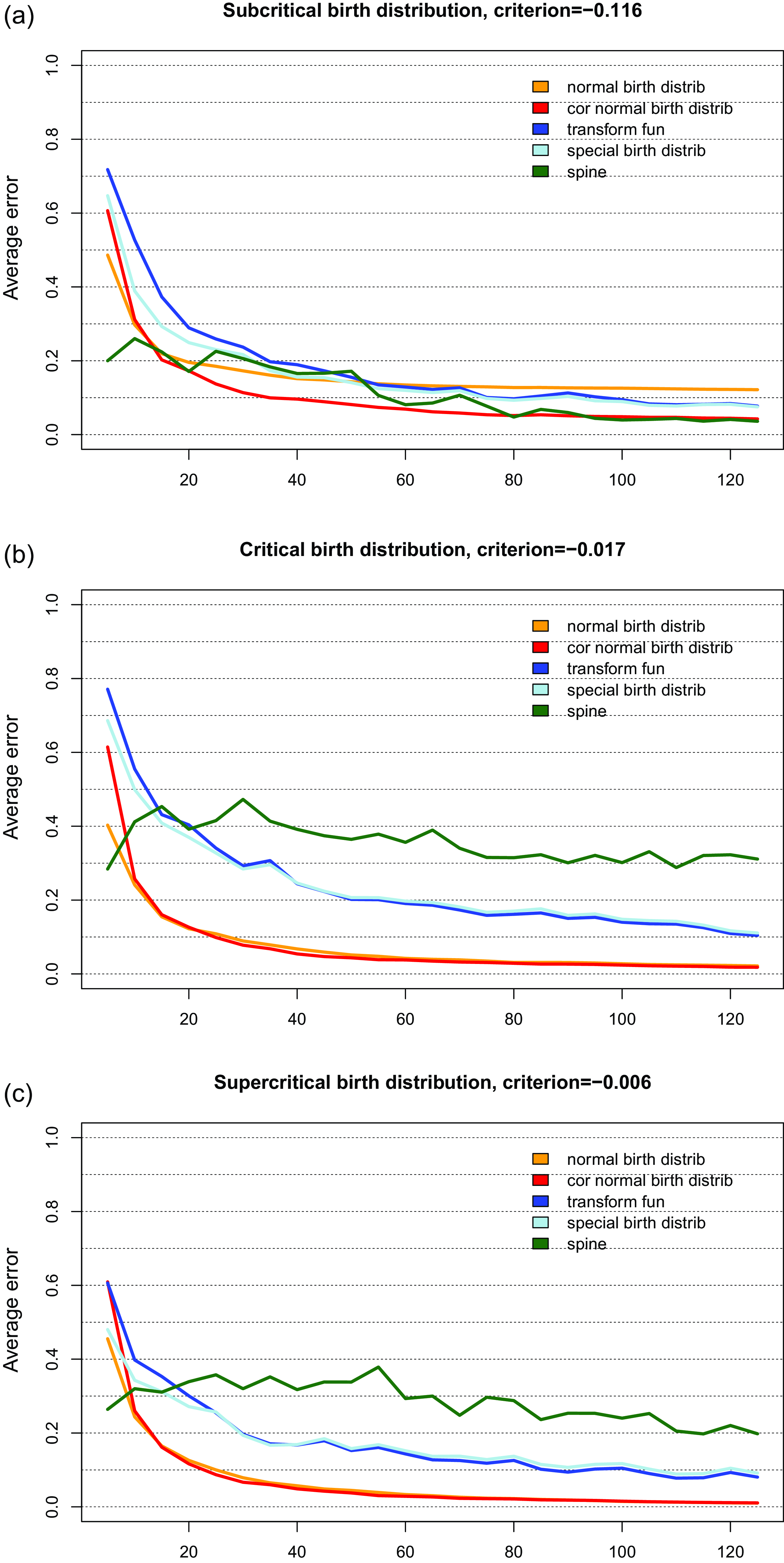
7.2. Asymptotic test of conditioned Galton–Watson trees
When observing a population modeled by a Galton–Watson tree, it is of primary importance to know whether or not it has been conditioned to survive, in particular when the birth distribution is subcritical. Here we show how the theoretical contributions of this paper can be used to develop an asymptotic test to answer this question.
We observe a subcritical tree T until generation h and would like to test the null hypothesis: T is a Galton–Watson tree conditioned to survive until (at least) generation h. In the framework of spinal-structured trees and approximating conditioned Galton–Watson trees by Kesten’s model [Reference Kesten10], this is equivalent to testing
 $f\propto\text{Id}$
, which simplifies the construction of the test but also provides a further motivation for the class of models considered in this paper. As in Section 7.1, we assume that
 $\sum_{i=0}^Nf(i)=1$
.
The construction of a test statistic for f requires both a consistent estimator and some knowledge of its asymptotic behavior. The latter is sorely lacking but can be estimated from numerical simulations. Here we restrict ourselves to binary (f(1) is therefore sufficient to know f) spinal-structured trees with
 $0.5\lt m(\mu)\lt 1$
and
 $0 \lt f(1) \lt 0.5$
, that is, f is increasing because
 $f(1)+f(2)=1$
. We suspect that
 $\widehat{f}_{h}(1)$
satisfies a central limit theorem with rate
 $\sqrt{h}$
. However, we want to check if this rate seems to be adequate, so we need to estimate its asymptotic variance, possibly as a function of both
 $\mu$
and f. To this end, we have estimated
 $h\operatorname{Var} (\widehat{f}_{h}(1)-f(1))$
from simulated samples of spinal-structured trees from various values of
 $\mu$
and f within the range specified above: the results are presented in Figure 3(a). First, we observe that
 $h\operatorname{Var} (\widehat{f}_{h}(1)-f(1))$
seems to be constant in h for any value of the two parameters, which validates the rate
 $\sqrt{h}$
. In addition, the asymptotic variance clearly depends on the parameters, but can be accurately predicted from them by a linear regression:
 \begin{equation*} \sigma^2(\mu,f) = 0.4611141 - 0.5561625\times m(\mu) + 1.0688165\times f(1).\end{equation*}
In Figure 3(b) we display the distribution of
 $\sqrt{h}(\widehat{f}_{h}(1)-f(1))/\sigma(\widehat{\mu}_{h},\widehat{f}_{h})$
, which is very close to the Gaussian distribution, as expected.
(a) Estimates of
 $h\operatorname{Var} (\widehat{f}_{h}(1)-f(1))$
from samples of 100 spinal-structured trees simulated with various parameters
 $\mu$
and f with
 $0.5 \lt m(\mu)\lt 1$
and
 $0\lt f(1)\lt 0.5$
, and (b) empirical distribution of the reduced centered error
 $\sqrt{h}(\widehat{f}_{h}(1)-f(1))/\sigma(\widehat{\mu}_{h},\widehat{f}_{h})$
for some of these parameters with a comparison to the Gaussian distribution (thick black line).

Relying on this short simulation study and recalling that
 $f(1)=1/3$
in Kesten’s model (
 $f\propto\text{Id}$
and
 $f(1)+f(2)=1$
), we introduce the test statistic
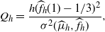 \begin{equation*}Q_h = \dfrac{h(\widehat{f}_{h}(1)-1/3)^2}{\sigma^2(\widehat{\mu}_{h},\widehat{f}_{h})},\end{equation*}
which approximately follows a
 $\chi^2(1)$
distribution when the underlying tree is sampled according to Kesten’s model. Denoting
 $\mathbf{q}(x) = \mathbb{P}(\chi^2(1) \gt x)$
, one rejects the hypothesis
 $f\propto\text{Id}$
with confidence level
 $1-\alpha$
when
 $Q_h \gt \mathbf{q}(1-\alpha)$
. Figure 4(a) illustrates the behavior of
 $Q_h$
when the tested hypothesis is true. Furthermore, Table 2 shows that the test rejects the null hypothesis with approximately the expected frequency of error
 $\alpha$
.
Empirical distribution of the test statistic
 $Q_h$
obtained from (a) samples of 100 Kesten’s trees with normal birth distribution
 $(0.55,0.2,0.25)$
, and (b) samples of 100 Galton–Watson trees with competition, both with a comparison to the
 $\chi^2(1)$
distribution (red line).

Empirical rejection rate measured when testing the null hypothesis
 $f\propto\text{Id}$
from samples of 100 Kesten’s trees with normal birth distribution
 $(0.55,0.2,0.25)$
observed until generation h for various levels of confidence
 $1-\alpha$
.

To go further, the behavior under the alternative hypothesis needs to be investigated. That is why we propose to apply the test to a population that does not follow Kesten’s model. For this purpose, we consider a Galton–Watson model with competition: for any
 $k\geq0$
, each node of the kth generation gives birth, with distribution
 $\mu_s$
depending on its size s, to a random number of children,
 \begin{equation*}\mu_{s} = \biggl( \dfrac{1}{4} \biggl(1-\dfrac{1}{s}\biggr), \dfrac{3}{4}\biggl(1-\dfrac{1}{s}\biggr) , \dfrac{1}{s}\biggr).\end{equation*}
It should be noted that
 $m(\mu_{s}) = {{3}/{4}} +{{5}/{(4s)}}$
, which makes the population growth supercritical when
 $s\leq 4$
, critical when
 $s=5$
, and subcritical when
 $s\geq6$
. Oscillating between exponential growth and decay, the population is likely to avoid extinction, without fitting to the behavior of a Galton–Watson tree conditioned on surviving. Figure 4(b) provides the distribution of the test statistic
 $Q_h$
under this model: it is significantly different from the
 $\chi^2(1)$
distribution expected under the null hypothesis, even from small populations, and thus differentiates from conditioned Galton–Watson trees.
Appendix. Proofs of intermediate lemmas
A.1. Proof of Lemma 5.1
Let
 $(x,y,z)\in\mathbf{F}(\alpha,\varepsilon)$
. The proof is based on the fact that if x, y, or z has some null coordinate, we may always perturb these points in order to decrease the objective function while still remaining in
 $\mathbf{F}(\alpha,\varepsilon)$
. For the sake of simplicity, we assume throughout the proof that
 $x_{i} \gt 0$
,
 $z_{i} \gt 0$
, and
 $y_{i} \gt 0$
, as soon as
 $i\neq0$
. The other cases can be treated similarly and are left to the reader. The harder case is when we have
 $x_{0}=z_{0}=0$
and
 $y_{0} \gt 0$
, but to give an example we first treat the case where
 $x_{0}=0$
,
 $z_{0} \gt 0$
and
 $y_{0} \gt 0$
. Henceforth, for any
 $X\in\mathbb{R}^{N+1}$
, we let I(X) denote the set given by
 \begin{equation*}I(X)=\{i\in[[0,N]] \mid X_{i}=0\},\end{equation*}
and let
 $\nabla^{+}d_{\textit{KL}}(x,p)$
be the vector given by
 \begin{equation*}\nabla^{+}d_{\textit{KL}}(x,p)=\begin{cases}1+\log(x_i/p_i)& \text{for all $ i\in I^{c}(x)$,}\\0& \text{for all $i\in I(x)$,}\end{cases}\end{equation*}
which is the vector of directional derivatives of
 $d_{\textit{KL}}(\cdot\,,p)$
in the directions where they are well-defined.
Case 1:
 $x_{0}=0$
,
 $z_{0} \gt 0$
and
 $y_{0} \gt 0$
. We first show that whenever
 $h\in \mathbb{R}^{N+1}$
satisfies
 $h_{0} \gt 0$
we have
 \begin{equation}\limsup_{\delta \to 0}\dfrac{f_{\alpha}(x+\delta h,y,z)-f_{\alpha}(x,y,z)}{\delta} \lt 0.\end{equation}
For any
 $i\in I(x)$
and any
 $\delta \gt 0$
,
 \begin{equation*}f_{\alpha}(x+\delta \mathbf{e}_{i},y,z)-f_{\alpha}(x,y,z)=(1-\alpha)\delta \log\biggl(\dfrac{\delta}{p_{i}} \biggr),\end{equation*}
where
 $\mathbf{e}_{i}$
is the ith vector of the canonical basis of
 $\mathbb{R}^{N+1}$
. This easily entails that
 \begin{equation}\lim_{\delta \to 0}\dfrac{f_{\alpha}(x+\delta \mathbf{e}_{i},y,z)-f_{\alpha}(x,y,z)}{\delta}=-\infty.\end{equation}
Now take
 $h\in \mathbb{R}^{N+1}$
such that
 $h_{0} \gt 0$
. We have that
 $h=h^{I(x)}+h^{I^c(x)}$
, where
 $h^{I(x)}$
is given by
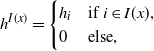 \begin{equation*}h^{I(x)}=\begin{cases}h_{i} & \text{if $i\in I(x)$,}\\0 & \text{else,}\end{cases}\end{equation*}
and
 $h^{I^c(x)}=h-h^{I(x)}$
. Thus, because f has well-defined directional derivatives in the direction of the positive coordinate, we have
 \begin{equation}f_{\alpha}(x+\delta h,y,z)=f_{\alpha}(x+\delta h^{I(x)},y,z)+\delta \nabla^{+}f_{\alpha}(x,y,z)\cdot h^{I^c(x)}+{\mathrm{o}} (\delta).\end{equation}
Thus (A.3) implies
 \begin{align*}& \limsup_{\delta \to 0}\dfrac{f_{\alpha}(x+\delta h,y,z)-f_{\alpha}(x,y,z)}{\delta}\\ &\quad = \limsup_{\delta \to 0}\dfrac{f_{\alpha}(x+\delta h^{I(x)},y,z)-f_{\alpha}(x,y,z)}{\delta}+\nabla^{+}f_{\alpha}(x,y,z)\cdot h^{I^c(x)},\end{align*}
and (A.1) now follows from (A.2). Now let
 $i^{\ast}\in [[ 0,N]]$
such that
 \begin{equation*}\log\biggl(\dfrac{(1-\alpha)x_{i^{\ast}}+\alpha z_{i^{\ast}}}{p_{i^{\ast}}} \biggr)=\min_{0\leq i\leq N}\log\biggl(\dfrac{(1-\alpha)x_{i}+\alpha z_{i}}{p_{i}} \biggr).\end{equation*}
Because
 $(1-\alpha)x+\alpha z\in\mathcal{M}$
and
 $p\in\mathcal{M}$
, we must have
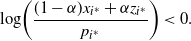 \begin{equation*}\log\biggl(\dfrac{(1-\alpha)x_{i^{\ast}}+\alpha z_{i^{\ast}}}{p_{i^{\ast}}} \biggr) \lt 0.\end{equation*}
Thus, taking
 $h= e_{0}-e_{i^{\ast}}$
, we get
 \begin{equation*}H_{\alpha,\varepsilon}(x+\delta h,y,z)-H_{\alpha,\varepsilon}(x,y,z)=\delta(1-\alpha)\biggl(\log\biggl(\dfrac{\alpha z_{0}}{p_{0}} \biggr)-\log\biggl(\dfrac{(1-\alpha)x_{i^{\ast}}+\alpha z_{i^{\ast}}}{p_{i^{\ast}}} \biggr)\biggr)+{\mathrm{o}}(\delta).\end{equation*}
For
 $\delta$
small enough, we obtain
 \begin{equation*}H_{\alpha,\varepsilon}(x+\delta h,y,z)\geq H_{\alpha,\varepsilon}(x,y,z),\end{equation*}
which implies that
 $(x+\delta h,y,z)\in\mathbf{F}(\alpha,\varepsilon)$
. In addition, (A.1) implies
 $f(x+\delta h,y,z) \lt f(x,y,z)$
for
 $\delta$
small enough. Thus (x,y,z) cannot be a solution of problem (P
α,ε
).
Case 2:
 $x_{0}=z_{0}=0$
and
 $y_{0} \gt 0$
. This particular case raises a new difficulty. Informally, in such a situation a perturbation of type
 $(x+\delta h,y,z+\delta \tilde{h})$
gives
 \begin{equation*}H_{\alpha,\varepsilon}(x+\delta h,y,z+\delta \tilde{h})=H_{\alpha,\varepsilon}(x,y,z)+\delta\log(\delta)+{\mathrm{o}} (\delta\log(\delta)).\end{equation*}
It follows that H is decreasing in any direction of type
 $\delta(h,0,\tilde{h})$
, and
 $(x+\delta h,y,z+\delta \tilde{h})$
may not be in
 $\mathbf{F}(\alpha,\varepsilon)$
. To overcome this problem, we consider perturbed points of the form
 \begin{equation*}\begin{cases}x^{\delta}=x+\delta \mathbf{e}_{0}-\delta \mathbf{e}_{i}+\delta\log(\delta)r,\\z^{\delta}=z+\delta \mathbf{e}_{0}-\delta \mathbf{e}_{i},\end{cases}\end{equation*}
where
 $r\in\mathbb{R}^{N+1}$
satisfies
 \begin{equation}\begin{cases}r_{0}=0,\\\sum_{i=0}^{N}r_{i}=0.\end{cases}\end{equation}
Thus, for sufficiently small
 $\delta$
, we have
 $z^{\delta}\in\mathcal{M}$
and
 $x^{\delta}\in\mathcal{M}$
. Because
 $x_{i} \gt 0$
and
 $z_{i} \gt 0$
for all
 $i \gt 0$
, we have
 \begin{equation*}d_{\textit{KL}}(x^{\delta},p)=d_{\textit{KL}}(x,p)+\delta\log(\delta)+\delta\log(\delta)r\cdot\nabla^{+}d_{\textit{KL}}(x,p)+{\mathrm{o}} (\delta\log(\delta))\end{equation*}
and
 \begin{equation*}d_{\textit{KL}}(z^{\delta},q)=d_{\textit{KL}}(z,q)+\delta\log(\delta)+{\mathrm{o}} (\delta\log(\delta)),\end{equation*}
which gives
 \begin{equation}f_{\alpha}(x^{\delta},y,z^{\delta})=f(x,y,z)+\delta\log(\delta)(1+(1-\alpha)r\cdot\nabla^{+}d_{\textit{KL}}(x,p))+{\mathrm{o}} (\delta\log(\delta)).\end{equation}
Similarly, we get
 \begin{align}&H_{\alpha,\varepsilon}(x^{\delta},y,z^{\delta})\nonumber\\&\quad =H_{\alpha,\varepsilon}(x,y,z)+\delta\log(\delta)(1+(1-\alpha)r\cdot\nabla^{+}d_{\textit{KL}}((1-\alpha)x+\alpha z,p))+{\mathrm{o}} (\delta\log(\delta)).\end{align}
Our next step is to show that for some choice of r and
 $\delta$
small enough, we have
 $f(x^{\delta},y,z^{\delta})\leq f(x,y,z)$
and
 $h(x^{\delta},y,z^{\delta})\geq h(x,y,z)$
, which imply
 $(x^{\delta},y,z^{\delta})\in \mathbf{F}(\alpha,\varepsilon)$
and that (x, y, z) is not a minimizer of f among the feasible set
 $\mathbf{F}(\alpha,\varepsilon)$
. To show this, by virtue of (A.5) and (A.6), we only need to find some
 $r\in\mathbb{R}^{N+1}$
satisfying conditions (A.4) and
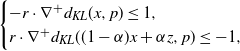 \begin{equation}\begin{cases}-r\cdot\nabla^{+}d_{\textit{KL}}(x,p)\leq 1,\\r\cdot\nabla^{+}d_{\textit{KL}}((1-\alpha)x+\alpha z,p)\leq -1,\end{cases}\end{equation}
in particular because
 $\delta\log(\delta) \lt 0$
for
 $\delta$
small enough. According to Farkas’s lemma, such an r exists as soon as there is no solution (u,v,w) to the problem
 \begin{equation}\begin{cases}-u\log\biggl(\dfrac{x_{i}}{p_{i}} \biggr)+v\log\biggl(\dfrac{(1-\alpha)x_{i}+\alpha z_{i}}{p_{i}} \biggr)+w=0\quad \text{for all $ i\gt 0$,}\\u-v \lt 0,\\u \gt 0,\ v \gt 0,\ w \gt 0.\end{cases}\end{equation}
Assume that (u,v,w) is a solution to problem (A.8). Thus, for all
 $i \gt 0$
,
 \begin{equation*}x_{i}={\mathrm{e}}^{{{w}/{u}}}p_{i}\biggl(\dfrac{(1-\alpha)x_{i}+\alpha z_{i}}{p_{i}}\biggr)^{{{v}/{u}}}.\end{equation*}
Hence, according to Jensen’s inequality and the conditions of problem (A.8),
 \begin{equation*}1={\mathrm{e}}^{{{w}/{u}}}\sum_{i=1}^{N}p_{i}\biggl(\dfrac{(1-\alpha)x_{i}+\alpha z_{i}}{p_{i}}\biggr)^{{{v}/{u}}}\geq {\mathrm{e}}^{{{w}/{v}}} \gt 1,\end{equation*}
which is absurd. Thus problem (A.8) has no solution, and Farkas’s lemma entails that there exists
 $r\in \mathbb{R}^{N+1}$
such that conditions (A.4) and (A.7) are satisfied.
The method is similar if we have more than one zero. This ends the proof.
A.2. Proof of Lemma 6.1
We begin the proof by showing that the Kullback–Leibler divergence
 $(q,p)\mapsto d_{\textit{KL}}(q,p)$
is locally Lipschitz in the second variable away from 0, and that this holds uniformly with respect to the first variable. We have
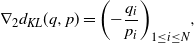 \begin{equation*}\nabla_{2}d_{\textit{KL}}(q,p)=\biggl(-\dfrac{q_{i}}{p_{i}} \biggr)_{1\leq i\leq N},\end{equation*}
where
 $\nabla_{2}$
denotes the gradient with respect to the second variable. Hence
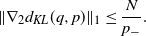 \begin{equation*}\|\nabla_{2}d_{\textit{KL}}(q,p)\|_{1}\leq \dfrac{N}{p_{-}}.\end{equation*}
Given
 $0 \lt \varepsilon \lt p_{-}$
, as soon as
 $\|p-\hat{p}\|_{1} \lt \varepsilon$
, we have
 \begin{equation*}\sup_{\{\hat{p}\in\mathcal{M}\,|\,\|p-\hat{p}\|_{1} \lt \varepsilon\}}\|\nabla_{2}d_{\textit{KL}}(q,\hat{p})\|_{1}\leq \dfrac{N}{p_{-}-\varepsilon},\end{equation*}
which entails that
 \begin{equation*}|d_{\textit{KL}}(q,p)-d_{\textit{KL}}(q,\hat{p})|\leq \dfrac{N}{p_{-}-\varepsilon}\|p-\hat{p}\|_1\quad\text{for all $ \hat{p}\in\mathcal{M}$ s.t. $\|p-\hat{p}\|_{1} \lt \varepsilon$.}\end{equation*}
To go further, we need to investigate the effect of a perturbation of p on
 $\mathcal{B}p$
, where the operator
 $\mathcal{B}$
was defined in (3.3). Now one can easily see that on the open set
 $\{p\in\mathcal{M}\mid m(p) \gt 1/2\}$
we have
 \begin{equation*}\|\nabla\mathcal{B}p\|_{1}\leq 2N.\end{equation*}
As
 $m(p)\geq1$
, there exists
 $\varepsilon \gt 0$
, such that
 $m(\hat{p}) \gt 1/2$
for all
 $\hat{p}\in B_{1}(p,\varepsilon)$
. Thus, for
 $\hat{p}\in \mathcal{M}\cap B_{1}(p,\varepsilon)$
, we have
 \begin{equation*}\|\mathcal{B}\hat{p}-\mathcal{B}p\|_{1}\leq 2N\|p-\hat{p}\|_{1},\end{equation*}
which ends the proof.
A.3. Proof of Lemma 6.2
First we have
 \begin{align}& \mathbb{P}(d_{\textit{KL}}(M+S,p)\gt d_{\textit{KL}}(R+S,p)) \nonumber \\&\quad = \sum_{r_{1}+\ldots+r_{N}=h-n}\sum_{m_{1}+\ldots+m_{N}=h-n}\sum_{s_{1}+\ldots+s_{N}=h} ((h-n)!)^2h!\prod_{i=1}^{N}\dfrac{p_{i}^{r_{i}}q_{i}^{m_{i}+s_{i}}}{r_{i}!m_{i}!s_{i}!}\mathbb{1}_{d_{\textit{KL}}(\bar{r},p)+\varepsilon \gt d_{\textit{KL}}(\bar{r},p)}. \end{align}
In addition, one can easily check that
 \begin{align*} \prod_{i=1}^{N}p_{i}^{r_{i}}q_{i}^{m_{i}+s_{i}} & = \exp(-(n-h)d_{\textit{KL}}(\bar{r},p)-(n-h)d_{\textit{KL}}(\bar{m},p)-hd_{\textit{KL}}(\bar{s},q))\\ & \quad \times \prod_{i=1}^{N}\biggl(\dfrac{r_{i}}{n-h}\biggr)^{r_{i}}\biggl(\dfrac{m_{i}}{n-h}\biggr)^{m_{i}}\biggl(\dfrac{s_{i}}{h}\biggr)^{s_{i}}.\end{align*}
In addition, since
 \begin{equation*}(h-n)!(h-n)! h!\prod_{i=1}^{N}(r_{i}!m_{i}!s_{i}!)^{-1}\prod_{i=1}^{N}\biggl(\dfrac{r_{i}}{n-h}\biggr)^{r_{i}}\biggl(\dfrac{m_{i}}{n-h}\biggr)^{m_{i}}\biggl(\dfrac{s_{i}}{h}\biggr)^{s_{i}}\leq 1,\end{equation*}
we obtain from (A.9) that
 \begin{align*}& \mathbb{P}(d_{\textit{KL}}(M+S,p) \gt d_{\textit{KL}}(R+S,p))\\ &\quad \leq \sum_{\begin{subarray} r_{1}+\ldots+r_{N}=h-n\\m_{1}+\ldots+m_{N}=h-n\\s_{1}+\ldots+s_{N}=h\end{subarray}} {\mathrm{e}}^{-(n-h)d_{\textit{KL}}(\bar{r},p)-(n-h)d_{\textit{KL}}(\bar{m},p)-hd_{\textit{KL}}(\bar{s},q)} \mathbb{1}_{d_{\textit{KL}}(\bar{r},p)+\varepsilon \gt d_{\textit{KL}}(\bar{r},p)},\end{align*}
which leads to
 \begin{equation*}\mathbb{P}(d_{\textit{KL}}(M+S,p) \gt d_{\textit{KL}}(R+S,p))\leq\dbinom{h-n+N-1}{N-1}^{2}\dbinom{h+N-1}{N-1}\exp(-hV(\alpha,\varepsilon)),\end{equation*}
where
 $V(\alpha,\varepsilon)$
is defined in (5.1) and
 $\alpha=h/n$
. Now, as
 \begin{equation*}\dbinom{h+N-1}{N-1}\leq {\mathrm{e}}^{N-1}\biggl(\dfrac{h+N-1}{N-1}\biggr)^{N-1}\leq C_{N}h^{N}\end{equation*}
for some constant
 $C_{N}$
, we get
 \begin{equation*}\mathbb{P}(d_{\textit{KL}}(M+S,p) \gt d_{\textit{KL}}(R+S,p))\leq C_{N}^{3}h^{3N}\exp({-}hV(\alpha,\varepsilon)).\end{equation*}
For any
 $\delta \gt 0$
, one can always find some constant (independent of h and
 $V(\alpha,\varepsilon)$
) such that
 \begin{equation*}C_{N}^{3}h^{3N}\exp({-}hV(\alpha,\varepsilon))\leq C \exp({-}h(V(\alpha,\varepsilon)-\delta)).\end{equation*}
This ends the proof.
Acknowledgements
The authors would like to thank the anonymous reviewers for their valuable comments that helped them to considerably improve the preliminary version of the paper. In particular, one of the reviewers pointed out an error in the proof of Theorem 5.1, which we corrected by following his/her suggestions.
Funding information
There are no funding bodies to thank relating to the creation of this article.
Competing interests
There were no competing interests to declare which arose during the preparation or publication process of this article.



