1 Introduction
Internal waves play an important role in ocean circulation. Generated by tides and winds, they propagate through the oceans and seas, redistributing momentum and energy before dissipating. The mechanism leading to dissipation and mixing remains to be clearly established but at least four possible dissipative processes are regularly invoked and still debated (Kunze & Llewellyn Smith Reference Kunze and Llewellyn Smith2004): wave–wave interactions and transfer to small scales through triadic resonant instability (MacKinnon & Winters Reference MacKinnon and Winters2005; Alford et al. Reference Alford, MacKinnon, Zhao, Pinkel, Klymak and Peacock2007; Dauxois et al. Reference Dauxois, Joubaud, Odier and Venaille2018), scattering by mesoscale structures (Rainville & Pinkel Reference Rainville and Pinkel2006), or by finite-amplitude bathymetry (Peacock et al. Reference Peacock, Mercier, Didelle, Viboud and Dauxois2009), and reflection on sloping boundaries, especially critical ones (Eriksen Reference Eriksen1982; Dauxois & Young Reference Dauxois and Young1999; Nash et al. Reference Nash, Kunze, Toole and Schmitt2004). In this context, the studies of reflections of internal waves on topographies are of particular interest since this dissipative mechanism may contribute to additional mixing of the ocean. In this paper, we will be particularly interested in three-dimensional (3D) reflection processes.
A usual simplification for the propagation of oceanic internal waves is to consider a non-rotating and stably stratified fluid with a linear stratification. This is a reasonable first approximation since the ratio of internal gravity wavelength over the (internal) Rossby deformation radius is usually small enough at the relevant scales for beamwise-propagating internal waves and also because we will consider reflections in closed domains, neglecting propagation over long distances. In this framework, Archimedes’ principle is quantified by the buoyancy frequency
 $N=\sqrt{(-g/\unicode[STIX]{x1D70C}_{0})\,\text{d}\overline{\unicode[STIX]{x1D70C}}/\text{d}z}$
, with
 $g$
the gravitational constant,
 $\unicode[STIX]{x1D70C}_{0}$
a constant reference density and
 $\overline{\unicode[STIX]{x1D70C}}(z)$
the unperturbed density field. The dispersion relation of internal waves in such a fluid is given by
 $\unicode[STIX]{x1D714}=\pm N\sin \unicode[STIX]{x1D703}$
, where
 $\unicode[STIX]{x1D703}$
is the angle of the direction of wave energy propagation with respect to the horizontal. One of the interesting consequences of this anisotropic dispersion relation is the preservation of the angle of propagation of an internal wave beam upon reflection at a rigid boundary.
The reflection on planar slopes in two dimensions has been extensively studied since Phillips (Reference Phillips1966) and is now well understood. Depending on the angle of propagation
 $\unicode[STIX]{x1D703}$
and the angle of the slope
 $\unicode[STIX]{x1D6FC}$
, reflections are divided into three categories. If
 $\unicode[STIX]{x1D703}<\unicode[STIX]{x1D6FC}$
, the reflection is subcritical, and the reflected beam propagates downwards (see figure 1
a). If
 $\unicode[STIX]{x1D703}>\unicode[STIX]{x1D6FC}$
, the reflection is supercritical, and the reflected beam propagates upwards (figure 1
c). In the critical case
 $\unicode[STIX]{x1D703}=\unicode[STIX]{x1D6FC}$
, following only the linear predictions, the beam could therefore be expected to propagate both upwards and downwards (figure 1
b): however, the amplitude of a reflected beam would be infinite. The singularity of this peculiar critical reflection has been healed by taking into account appropriately transience, nonlinearity and viscous effects (Dauxois & Young Reference Dauxois and Young1999; Tabaei, Akylas & Lamb Reference Tabaei, Akylas and Lamb2005).
Schematic representation of the possible reflections that can occur when a linear internal wave beam is propagating in two dimensions. (a) Subcritical reflection. (b) Critical reflection. (c) Supercritical reflection. At the bouncing point, the St Andrew’s cross is plotted in grey. The incident and reflected rays are respectively plotted in green and red.

Given these bouncing linear rules, one can easily compute the path of an internal wave beam in a given geometry. These trajectories are very different from what we are used to with acoustic or optical waves, nearly always leading to internal wave attractors. In a given geometry, an internal wave attractor is indeed a path towards which all internal waves of a given frequency will converge: this is therefore a limit cycle although only the linear dispersion relation is used. It has been tested through ray tracing that this attracting structure exists in various geometries (Maas & Lam Reference Maas and Lam1995; Maas Reference Maas2005; Hazewinkel, Maas & Dalziel Reference Hazewinkel, Maas and Dalziel2011; Brouzet et al. Reference Brouzet, Sibgatullin, Scolan, Ermanyuk and Dauxois2016b ). Once the geometry is given, the domain of existence of attractors corresponds to a large region of the parameter space describing the geometry (Maas et al. Reference Maas, Benielli, Sommeria and Lam1997; Maas Reference Maas2005; Brouzet et al. Reference Brouzet, Ermanyuk, Joubaud, Pillet and Dauxois2017). These arguments underline the possibility that appropriate conditions to get wave attractors can be encountered in the ocean (Buhler & Muller Reference Buhler and Muller2007; Guo & Holmes-Cerfon Reference Guo and Holmes-Cerfon2016). If this is the case, wave attractors may play an important role in the mixing. Indeed, since the internal waves of a given geometry should converge onto one single path, the energy on this path when not hindered by viscosity will lead to nonlinear effects and therefore to mixing events (Bourget et al. Reference Bourget, Scolan, Dauxois, Le Bars, Odier and Joubaud2014; Brouzet et al. Reference Brouzet, Ermanyuk, Joubaud, Sibgatullin and Dauxois2016a , Reference Brouzet, Sibgatullin, Ermanyuk, Joubaud and Dauxois2017).
Internal wave attractors have been extensively studied theoretically (Maas & Lam Reference Maas and Lam1995; Ogilvie Reference Ogilvie2005; Lam & Maas Reference Lam and Maas2008), numerically (Rieutord, Georgeot & Valdettaro Reference Rieutord, Georgeot and Valdettaro2001; Grisouard, Staquet & Pairaud Reference Grisouard, Staquet and Pairaud2008) and experimentally (Hazewinkel et al. Reference Hazewinkel, van Breevoort, Dalziel and Maas2008, Reference Hazewinkel, Tsimitri, Maas and Dalziel2010) in two dimensions, but no clear evidence of attractors has been found in the ocean yet (Manders, Maas & Gerkema Reference Manders, Maas and Gerkema2004). Internal wave attractors in 3D geometries have been much less studied (Manders & Maas Reference Manders and Maas2003; Drijfhout & Maas Reference Drijfhout and Maas2007; Hazewinkel et al. Reference Hazewinkel, Maas and Dalziel2011). The aim of this article is precisely to study these attractors in 3D geometries. In this paper, we will focus only on the simplest attractors, for which the path formed by the attractor is a quadrilateral having one single reflection at the surface and one at the sidewall, a (1,1)-attractor. For the sake of simplicity, in the remainder of the paper, we will not repeat that we discuss (1,1)-attractors only and simply refer to them as ‘attractors’. To simplify further, we will conduct our study through two geometries which slightly vary from the two-dimensional (2D) case.
(i) The 2D attractor-like set-up. This geometry is one of the simplest to obtain 2D attractors and has been extensively investigated. It consists of a right trapezium prism with given height
 $H$
, length
$L$
and width
$W$
, and a single sloping wall of tunable inclination. Usually, the precise width has no influence and the geometry is considered to be quasi-2D. In this paper, we not only take a large value of
$W$
, to be in a fully 3D case, but also we will apply the forcing over a limited stretch in the transverse direction only, potentially leading to 3D effects.
(ii) The canal-like set-up. A long but narrow tank is taken to mimic a canal while a sloping bottom is used to simply represent the most essential feature of the topography. Again here, the slope angle
$\unicode[STIX]{x1D6FC}$
with the horizontal can be tuned. The waves are forced by the generator in the along-canal lateral direction, parallel to the slope. Moreover, forcing always takes place over a limited stretch of the tank’s width only.


With these two experimental set-ups, we will be able to study carefully the robustness of internal wave attractors when a third dimension cannot be overlooked. In § 2, we first discuss the reflection and the refractive focusing that appear in three dimensions. In § 3, we present the results of the quasi-2D set-up, first with simple ray tracing, and then both experimentally as well as numerically. In § 4, we introduce the experiment with the canal-like geometry where the refractive focusing leads to counter-intuitive and striking wave trapping in the transverse plane. Likewise, we start with ray tracing predictions before discussing the experimental results. Finally, in § 5, we conclude and draw some perspectives.
2 Propagation and focusing in three dimensions
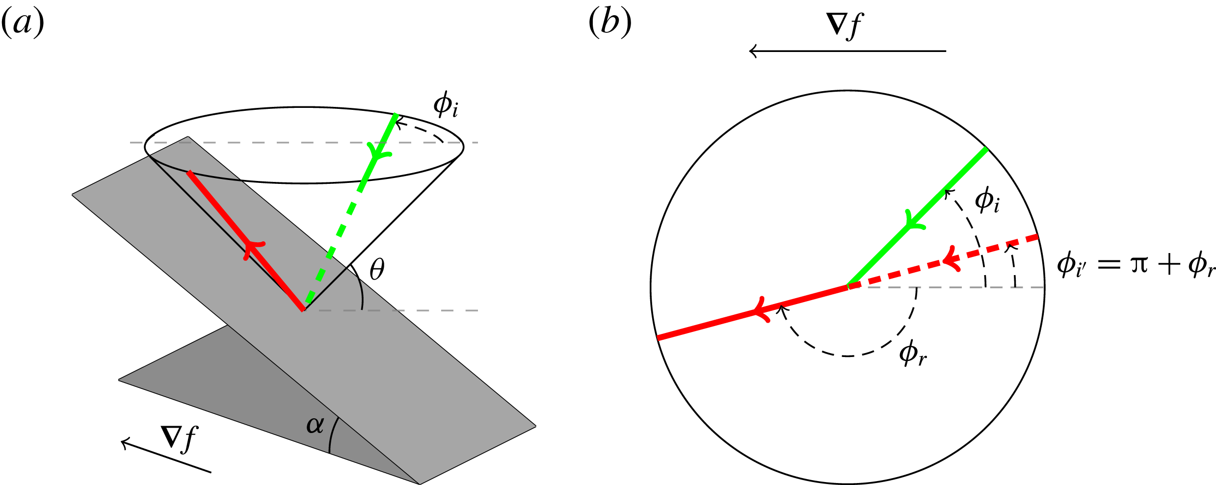
In 3D geometries, the propagation and reflection laws are more complex than in two dimensions. The St Andrew’s cross, generally used for describing 2D propagation, is transformed into a double cone whose aperture is given by the angle of propagation
 $\unicode[STIX]{x03C0}/2-\unicode[STIX]{x1D703}$
. An internal wave is then constrained to propagate on the cone. But of course, besides
 $\unicode[STIX]{x1D703}$
, another angle
 $\unicode[STIX]{x1D719}$
is needed to describe the position of the ray on the cone (see figure 2).
When reflection off a boundary occurs, the reflected ray must stay on the cone, but the horizontal propagation direction of the incident ray,
 $\unicode[STIX]{x1D719}_{i}$
, measured relative to the downslope direction, changes. The horizontal propagation direction of the reflected wave ray,
 $\unicode[STIX]{x1D719}_{r}$
, can be calculated given that of the incident wave ray, angle
 $\unicode[STIX]{x1D719}_{i}$
. This occurs according to the following law of refraction,
 $$\begin{eqnarray}\sin \unicode[STIX]{x1D719}_{r}={\displaystyle \frac{(s^{2}-1)\sin \unicode[STIX]{x1D719}_{i}}{2s\cos \unicode[STIX]{x1D719}_{i}+s^{2}+1}},\end{eqnarray}$$
derived for a single reflection by Phillips (Reference Phillips1963), and reformulated and applied iteratively by Maas (Reference Maas2005). Here,
 $s(x,y,z)=\tan \unicode[STIX]{x1D6FC}/\tan \unicode[STIX]{x1D703}$
represents the local slope of the topography,
 $\tan \unicode[STIX]{x1D6FC}$
, normalized by the characteristic slope,
 $\tan \unicode[STIX]{x1D703}$
, while the bottom is
 $z=f(x,y)$
, whose slope is given by
 $\tan \unicode[STIX]{x1D6FC}=[f_{x}^{2}+f_{y}^{2}]^{1/2}$
and subscripts denote differentiation. This formula is obtained by taking into account the dispersion relation of internal waves and the impermeability condition when internal waves reflect from bottom, surface, sidewall or slope. An example of a ‘supercritical’ 3D reflection is sketched in figure 2.
Perspective view (a) and top view (b) of the reflection of an internal wave beam off an inclined slope
 $z=f(x,y)$
. The bottom, inclined at angle
 $\unicode[STIX]{x1D6FC}$
with respect to the horizontal
 $xy$
-plane, is represented by the inclined grey rectangle, and its upslope-directed gradient is given by the horizontal vector
 $\unicode[STIX]{x1D735}f=(f_{x},f_{y},0)$
. The internal wave beam propagates along a cone whose inclination,
 $\unicode[STIX]{x1D703}$
, is set by the ratio of wave and stability frequencies. The incident (in green) and reflected (in red) beams make angles
 $\unicode[STIX]{x1D719}_{i}$
and
 $\unicode[STIX]{x1D719}_{r}$
relative to the downslope direction, respectively (beams are solid when visible while dashed if not).

This law of reflection gives birth to a whole class of behaviour absent in 2D geometries. After bounces on vertical and horizontal walls, the ray may come back on the inclined slope, but this time with a new incident angle
 $\unicode[STIX]{x1D719}_{i}^{\prime }=\unicode[STIX]{x03C0}+\unicode[STIX]{x1D719}_{r}$
measured with respect to the upslope direction. In some cases, this new angle is smaller than the incident one,
 $\unicode[STIX]{x1D719}_{i}$
, meaning that the angle of propagation will converge to
 $0^{\circ }$
after numerous bounces from surface and sloping bottom. This is the refractive focusing pointed out by Maas (Reference Maas2005). Given the definition of the angle
 $\unicode[STIX]{x1D719}$
, it means that upon multiple surface and subsequent slope reflections the ray will eventually propagate perpendicular to the slope considered.
Internal wave trapping at a finite distance from the emission point, in a plane transverse to the direction into which these waves are launched, may seem paradoxical. Upon a focusing reflection, wavelength and group speed of a reflecting internal wave decrease. Hence, when the internal wave refracts towards the transverse direction, its energy propagation slows down and, in the ideal fluid description, comes to a halt when that wavelength vanishes. This does not imply, however, that the (oscillatory) fluid motion is confined in the down-canal direction; it is merely reoriented upslope. Moreover, when the internal wave scale decreases due to (repeated) geometric focusing, at some point focusing is physically controlled by viscous and/or nonlinear processes.
The ray advancing into the fluid domain, first propagating completely parallel to the slope, when being diverted upslope, will seemingly slow down. This is because the velocity parallel to the ray will increase in magnitude in cross-slope direction, but not in down-canal direction. Hence, the computation of subsequent reflections will be more and more dominated by these increasing cross-canal speeds until, when the ratio to the down-canal velocity approaches infinity, the ray comes to a complete standstill in the down-canal direction.
3 The two-dimensional attractor-like geometry
3.1 Ray tracing prediction
In order to have an idea of the path of the internal waves in a 3D geometry, one can simply rely on ray tracing. In a linearly stratified fluid, internal waves propagate along straight lines. Given the coordinates of the point from which the wave ray is sent to the slope, and the initial values for angles (
 $\unicode[STIX]{x1D719}_{0}$
,
 $\unicode[STIX]{x1D703}$
), one can compute the location of the bottom reflection and the local bottom slope,
 $s$
. Then, using (2.1), one can determine angle
 $\unicode[STIX]{x1D719}_{r}$
of the reflected beam. This allows computation of the location of the next surface reflection, and subsequent horizontal propagation direction,
 $\unicode[STIX]{x1D719}_{0}^{\prime }=\unicode[STIX]{x1D719}_{r}+\unicode[STIX]{x03C0}$
. Iterating this process several times, one obtains the path an internal ray beam follows, as shown, for example, by Rabitti & Maas (Reference Rabitti and Maas2013, Reference Rabitti and Maas2014). They mainly focused on spherical and spherical shell geometries but a simple canal in a rotating fluid has also been studied experimentally and by ray tracing (Manders & Maas Reference Manders and Maas2004). In each case, they found that, for a given range of parameters, the internal ray, thanks to the focusing effect described in the previous section, ends up forming an attractor which is confined to a plane and thus identical to 2D attractors.
Brouzet et al. (Reference Brouzet, Ermanyuk, Joubaud, Sibgatullin and Dauxois2016a
,Reference Brouzet, Sibgatullin, Scolan, Ermanyuk and Dauxois
b
) have studied 2D attractors in a trapezoidal geometry, which are easy to set up experimentally. The tank used in these studies was 350 mm high, 600 mm long and quite narrow, only 170 mm wide. More importantly, the wave generator was, on purpose, almost as wide as the tank’s width. The two-dimensionality of the attractors in such a geometry was checked carefully by Brouzet et al. (Reference Brouzet, Sibgatullin, Scolan, Ermanyuk and Dauxois2016b
). Our first goal is thus to see what happens to this attractor in a tank that is much wider (
 $W=800$
mm) than the width of the forcing device (150 mm), changing it into a genuine 3D problem. Indeed, we re-used the same generator as for the 2D case. The slope with a tunable angle
 $\unicode[STIX]{x1D6FC}$
is placed along the whole width of the tank (as in the 2D set-up).
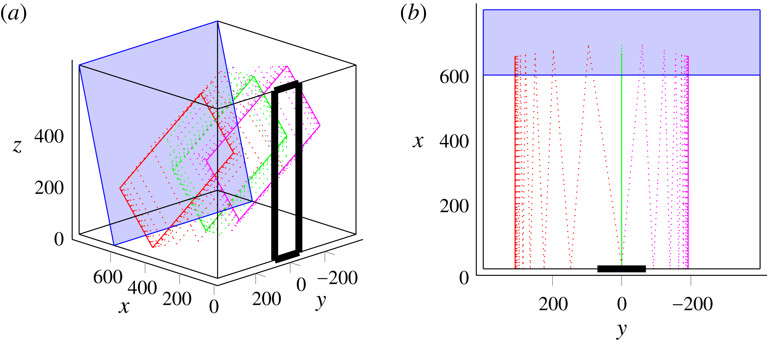
We performed ray tracing in this geometry. For rays sent exactly along the cross-slope
 $x$
-direction, i.e.
 $\unicode[STIX]{x1D719}_{0}=0^{\circ }$
, we recover exactly the 2D case: as expected, attractors are created in
 $xz$
-planes, with
 $y$
-values identical to those of the initial rays. This is shown in figure 3(a), in which the green ray represents a wave sent with
 $\unicode[STIX]{x1D719}_{0}=0^{\circ }$
: the ray path sticks to a transverse plane.
Now if we change the
 $\unicode[STIX]{x1D719}_{0}$
-value, meaning we send rays with a small angle with respect to the
 $x$
-axis, the red ray path in figure 3(a) shows that the trajectory is not 2D any more. The ray path is clearly 3D, but, due to the focusing effect described in § 2, the component of the ray along the width is reduced at every bounce against the slope and we end up with a trajectory confined to a transverse
 $xz$
-plane. The final
 $y$
-values of these planes depend in a non-trivial way on the initial position of the ray beam, but also on the initial angle
 $\unicode[STIX]{x1D719}_{0}$
.
Figure 3(b) shows the tank from above so that we can clearly see if the propagation is bounded in a
 $xz$
-plane or not. By contrast, this representation does not allow us to see that the paths in the
 $xz$
-planes are attractors.
The 2D attractor-like geometry: perspective (a) and top (b) views. The slope is represented by the inclined blue rectangle, while the generator is sketched by the thick vertical rectangle in the
 $x=0$
plane, stretching from
 $y=-70$
to
 $y=70$
. In both panels, dimensions are in mm. The successive reflections of three different incident rays are then represented with different colours: rays sent with
 $\unicode[STIX]{x1D719}_{0}=0^{\circ }$
in green,
 $\unicode[STIX]{x1D719}_{0}=7^{\circ }$
in red and
 $\unicode[STIX]{x1D719}_{0}=-5^{\circ }$
in magenta. The three rays start at the same initial position, given by
 $y_{0}=W/2$
and
 $z_{0}=H/2$
. For clarity of the demonstration, we choose the set of input values to ensure that focusing is slow and more visible in the graphic representation. Similar calculations for the experimental set of parameters would yield faster focusing.

Introducing the experimental parameters in the ray tracing programme, we found that an angular spread of only
 $\unicode[STIX]{x1D719}_{0}=0^{\circ }\pm 5^{\circ }$
is sufficient to get attractors created everywhere transversely throughout the tank. Moreover, as the geometry is transversely invariant (only the forcing is not), and the frequency given, the final attractors are all identical, but in different transverse
 $xz$
-planes.
In the experimental set-up, even if the waves are forced theoretically with
 $\unicode[STIX]{x1D719}_{0}=0^{\circ }$
, a diffraction-like phenomenon can be expected for the angle
 $\unicode[STIX]{x1D719}_{0}$
, as obtained previously when this generator was used in a tank significantly wider than the generator (Gostiaux et al.
Reference Gostiaux, Didelle, Mercier and Dauxois2007; Bordes Reference Bordes2012). So we expect to see experimentally attractors along the whole tank width, while the forcing only occurs at its centre.
3.2 Experiments
3.2.1 Material and methods
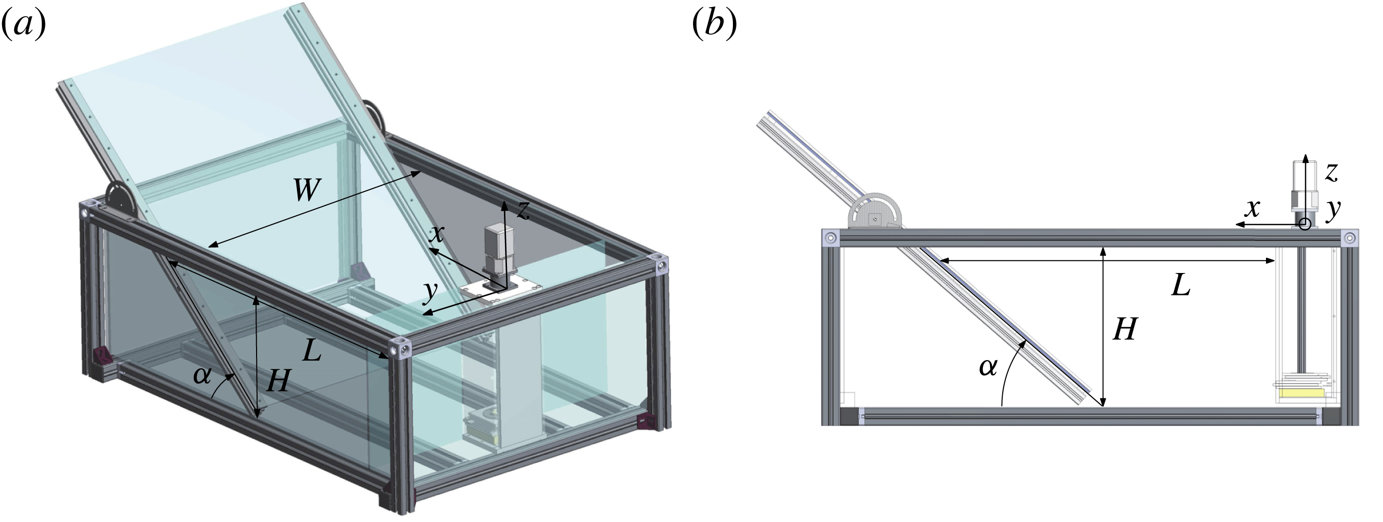
The tank used for this first experiment is sketched in figure 4. Its size is
 $1200~\text{mm}\times 800~\text{mm}\times 400~\text{mm}$
. The length,
 $L$
, at the top of the tank in between slope and wavemaker and the slope inclination
 $\unicode[STIX]{x1D6FC}$
are tunable. The tank is filled with a uniformly stratified fluid using the double-bucket technique (Oster & Yamamoto Reference Oster and Yamamoto1963) with salt used as a stratifying agent. The density profile is measured with a conductivity probe attached to a vertical traverse mechanism. The value of the buoyancy frequency is then evaluated from the measured density profile. The typical value is
 $N=0.95\pm 0.05~\text{rad}~\text{s}^{-1}$
.
The 2D attractor-like geometry: perspective (a) and top (b) views of the experimental set-up. The retractable slope and the wave generator are visible. The parameters used for our experiment are
 $H=320~\text{mm}$
,
 $L=570~\text{mm}$
,
 $W=800~\text{mm}$
and
 $\unicode[STIX]{x1D6FC}=57^{\circ }$
.

The forcing is created by the internal wave generator developed by Gostiaux et al. (Reference Gostiaux, Didelle, Mercier and Dauxois2007), studied by Mercier et al. (Reference Mercier, Martinand, Mathur, Gostiaux, Peacock and Dauxois2010) and later improved by Bordes (Reference Bordes2012). It consists of a stack of 47 plates to which we can change the amplitude and phase of oscillations, that are linked by an Archimedes’ screw. Thus, the time-dependent vertical profile of the generator can be tuned to create different profiles. For this experiment, we force with the first vertical mode of internal waves. The profile is thus given by
 $$\begin{eqnarray}\unicode[STIX]{x1D701}(z,t)=a\sin (\unicode[STIX]{x1D714}t)\cos (\unicode[STIX]{x03C0}z/H),\end{eqnarray}$$
where
 $a$
is the amplitude of motion of the cams and
 $\unicode[STIX]{x1D714}$
is the frequency of the forcing.
Since we are interested in 3D effects, we cannot use the synthetic schlieren method (Dalziel, Hughes & Sutherland Reference Dalziel, Hughes and Sutherland2000) often used for internal wave measurements when the fluid displacements are 2D to a good approximation. Consequently, here, internal wave beams are visualized using the particle image velocimetry (PIV) technique (Tropea, Yarin & Foss Reference Tropea, Yarin and Foss1973). We record the displacement of particles illuminated by a laser sheet. The particles are silver-coated spheres of size
 $10~\unicode[STIX]{x03BC}\text{m}$
and density
 $1400~\text{kg}~\text{m}^{-3}$
. The sedimentation velocity is found to be very low compared to the other velocities at play: it will have no consequences. Using a cross-correlation technique (Fincham & Delerce Reference Fincham and Delerce2000), we can finally deduce the velocity field in the tank from these images. The mesh of measurements is found to be sufficient to resolve the small-scale details of the wave field.
In a second treatment, the Hilbert transform is used to reduce noise. This method, first applied to internal waves by Mercier, Garnier & Dauxois (Reference Mercier, Garnier and Dauxois2008), is now widely used in the internal wave community. The method consists of three steps. First, a temporal Fourier transform is performed on the signal. Second, a temporal filter is applied. Finally, an inverse Fourier transform makes it possible to obtain the filtered field. Generally, the filter is centred around the forcing frequency
 $f=2\unicode[STIX]{x03C0}/\unicode[STIX]{x1D714}$
but it can be used in the case of triadic resonance and/or wave turbulence to study simultaneously several waves of different frequencies (Bourget et al.
Reference Bourget, Dauxois, Joubaud and Odier2013; Brouzet et al.
Reference Brouzet, Ermanyuk, Joubaud, Sibgatullin and Dauxois2016a
). Another common use of the Hilbert transform is to filter the signal spatially. For instance, one can separate waves propagating towards positive
 $x$
-values from waves propagating towards negative
 $x$
-values. Both spatial and temporal filtering can be simultaneously applied, as will be done in the remainder of this article.
For this experiment, a laser sheet, created above the tank, illuminates a
 $xz$
-plane along the tank. The laser sheet can be easily translated to obtain different slices of the tank, for different
 $y$
-values. A computer-controlled video AVT (Allied Vision Technologie) Pike camera with charge-coupled device (CCD) matrix of
 $1382\times 1034~\text{pixels}$
is used for video recording. The camera is located at a distance 1600 mm from the tank and operates at a constant frame rate of
 $2$
Hz, which is sufficient to resolve the significant frequencies of the signal (typically of the order of 0.1 Hz) and large enough so that the particles stay within the laser sheet between two images.
3.2.2 Experimental results
We performed experiments for the 2D attractor-like geometry with a mode-1 forcing (3.1) with
 $a=5$
mm. For the longitudinal geometry, we have chosen the same parameters as used by Brouzet et al. (Reference Brouzet, Ermanyuk, Joubaud, Sibgatullin and Dauxois2016a
). However, the forcing applies only on 150 mm out of 800 mm. We therefore expect to see the same attractors in the middle of the tank (where the forcing occurs) and, according to the ray tracing prediction, away from the forcing region as well.
Let us consider first the steady state. Once the generator is started, one waits long enough (typically 100 periods) to reach the steady state of the attractor. We then record the displacements of the particles in different
 $xz$
-slices, from the centre of the tank to one edge (
 $y$
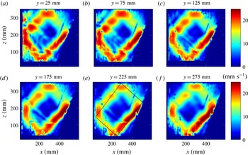
varying from 0 to 400 mm). Figure 5 shows the velocity field obtained after Hilbert filtering at the forcing frequency
 $\unicode[STIX]{x1D714}$
.
Filtered norm velocity for different
 $y$
-positions indicated above each panel. As an example, for panel (e), the ray tracing prediction is plotted with a solid black line, using the experimental parameters:
 $L=360~\text{mm}$
,
 $W=800~\text{mm}$
,
 $H=320~\text{mm}$
,
 $\unicode[STIX]{x1D6FC}=57^{\circ }$
,
 $N=1.14~\text{rad}~\text{s}^{-1}$
and
 $\unicode[STIX]{x1D714}=0.515~\text{rad}~\text{s}^{-1}$
.

One can see in figure 5 that, even if the forcing is only centred on a small part of the tank, the velocity field is almost the same everywhere throughout the tank, showing a nice attractor velocity field. We checked the presence of attractors on both sides of the tank. Because of light absorption, the signal is better when the slice is close to the camera; this is why we only show here the slices for positive values of
 $y$
.
Figure 5 shows the existence of attractors everywhere in the tank, but does not exhibit the appropriate mechanism for the transverse spreading. One could first argue that attractors away from the forcing can only be due to viscous diffusion from the centre of the tank towards the sidewalls. If so, we would see an important time dependence of the appearance of attractors with distance from the centre of the tank. An order-of-magnitude estimate of viscous spreading of the attractor is given by
 $y=\sqrt{\unicode[STIX]{x1D708}t}$
. For the viscosity of water
 $\unicode[STIX]{x1D708}\simeq 10^{-6}~\text{m}^{2}~\text{s}^{-1}$
and a distance from the centre
 $y=300$
mm, one obtains an estimate of the propagation time of the central velocity field of
 $T\simeq 10^{5}~\text{s}$
, or, approximately
 $T=10^{4}T_{0}$
.
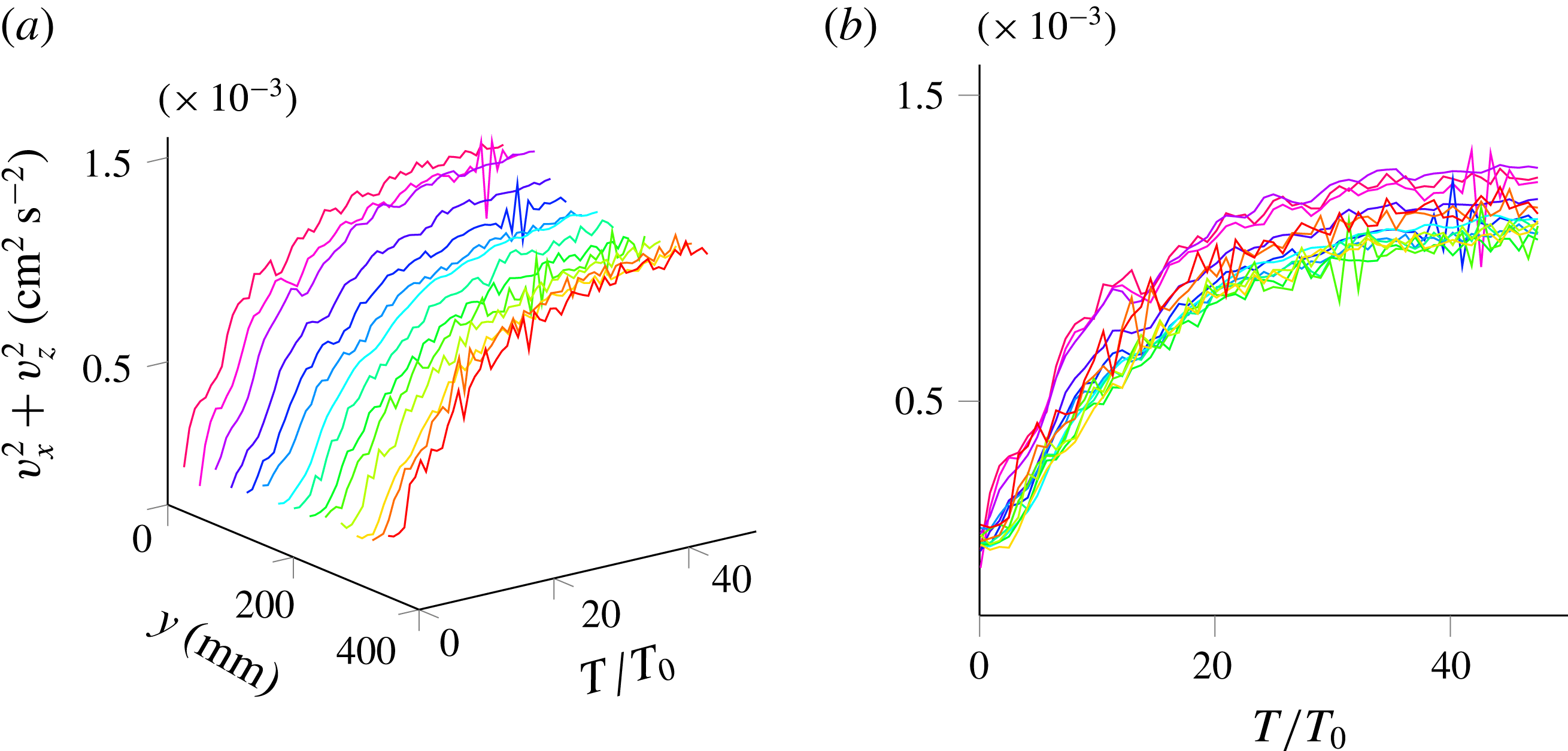
We hence performed a second series of measurements, focusing on the transitory regime of the attractors in each slice to see if such a large shift is observed between the time to reach the attractor steady state. For each slice, we started the camera acquisition and the generator at the same time. Before analysing, we perform an empirical mode decomposition (EMD) on the signal. This method, described in Huang et al. (Reference Huang, Shen, Long, Wu, Shih, Zheng, Yen, Tung and Liu1998) and Rilling & Flandrin (Reference Rilling and Flandrin2009), allows one to decompose the signal in the sum of all the important frequency contributions. In the present experiment, since we are interested only in the transitory regime, it allows us to get rid of high frequencies. In this experiment, strong oscillations at the forcing frequency are indeed present. As explained in Brouzet et al. (Reference Brouzet, Ermanyuk, Joubaud, Pillet and Dauxois2017), these oscillations are due to the propagating or standing nature of the waves and are not of interest here, since they do not modify the time scale of the transitory regime. We then looked at the sum of the squared longitudinal velocity amplitudes,
 $v_{x}^{2}+v_{z}^{2}$
. Figure 6 presents its time series for every slice. We can clearly see that the steady state is reached after approximately the same transient time for each slice, hence invalidating the intuitive mechanism of attractor spreading along the width of the tank by viscous diffusion. The rapid propagation of wave energy through the tank and its relative homogeneity in the steady state both strongly support spreading by wave propagation followed by refractive trapping.
Time evolution of the squared longitudinal velocity amplitude for different transverse slices of the tank. A different colour is used for the 14 different
 $y$
-slices varying from 0 to 350 mm. (a) Perspective view. (b) Side view. The oscillations at the forcing frequency have been removed using EMD.

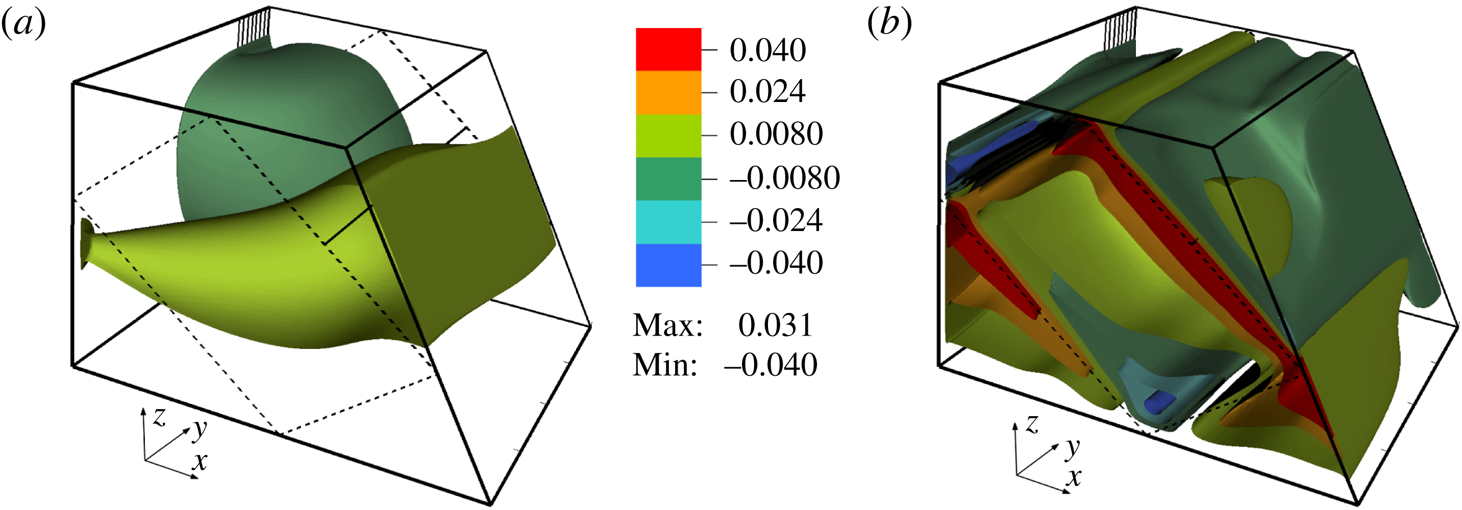
Perspective views of the attractors with the contours of the vertical velocity at
 $t=16$
s (a) and
 $t=2504.5$
s (b). The simulation results correspond to the following parameters:
 $L=456$
mm,
 $W=800$
mm,
 $H=308$
mm,
 $\unicode[STIX]{x1D6FC}=60^{\circ }$
,
 $N=0.948~\text{rad}~\text{s}^{-1}$
and
 $\unicode[STIX]{x1D714}=0.589~\text{rad}~\text{s}^{-1}$
. The generator, sketched by the vertical lines at the back of the figure, had an amplitude
 $a=0.6$
mm. The dashed lines drawn on the sides of the domain correspond to the theoretical skeleton of the wave attractor predicted by the ray tracing. The horizontal solid line connecting the middles of the first rays on the opposite lateral sides shows the location of the transverse cut for which we show below the transverse distribution of the cross-correlations and amplitudes of the wave motion.

3.3 Numerical simulations
To have a complementary view of the above results, we have performed direct numerical simulations. We used a well-tested spectral element approach, a version of the Nek5000 code (Fischer Reference Fischer1997; Fischer & Mullen Reference Fischer and Mullen2001). Using this code, 3D numerical modelling of a quasi-2D laboratory set-up, described in Brouzet et al. (Reference Brouzet, Sibgatullin, Scolan, Ermanyuk and Dauxois2016b
), showed excellent correspondence to the experiments (see also Brouzet et al.
Reference Brouzet, Ermanyuk, Joubaud, Sibgatullin and Dauxois2016a
). Results of direct numerical simulations of the present problem are found to be similar to the experimental results. The initial stage of the transient process of the wave field formation is depicted in figure 7(a) with the help of contours of the vertical component of velocity. The amplitude of the wavemaker was chosen to be sufficiently small to ensure the attractor is in the linear regime. Only half of the domain is shown in spanwise direction and, to visualize the internal flow structure, we have cut off the near-wall region
 $y>390$
mm. The ratio of the wavemaker width to the whole width of the tank is the same as in the experiments. As could be expected, the wave perturbations propagate from the wavemaker over a wide range of azimuthal directions. The dashed lines drawn on the sides of the domain correspond to the theoretical skeleton of the wave attractor predicted by the ray tracing. The horizontal solid line connecting the middles of the first rays on the opposite lateral sides shows the location of the transverse cut for which we show below the transverse distribution of the cross-correlations and amplitudes of the wave motion. Below, this line is referred to as the ‘probe line’. Figure 7(b) presents the isosurfaces of the vertical component of velocity after 235 periods of the wavemaker oscillations. Note that we use the same colour bar in both panels of figure 7. It is clearly seen that the isosurfaces form a structure that is close to a 2D one. At the same time, noticeable deviations from a purely 2D structure are visible: interestingly, the velocity may increase in transverse direction towards the lateral sidewall.
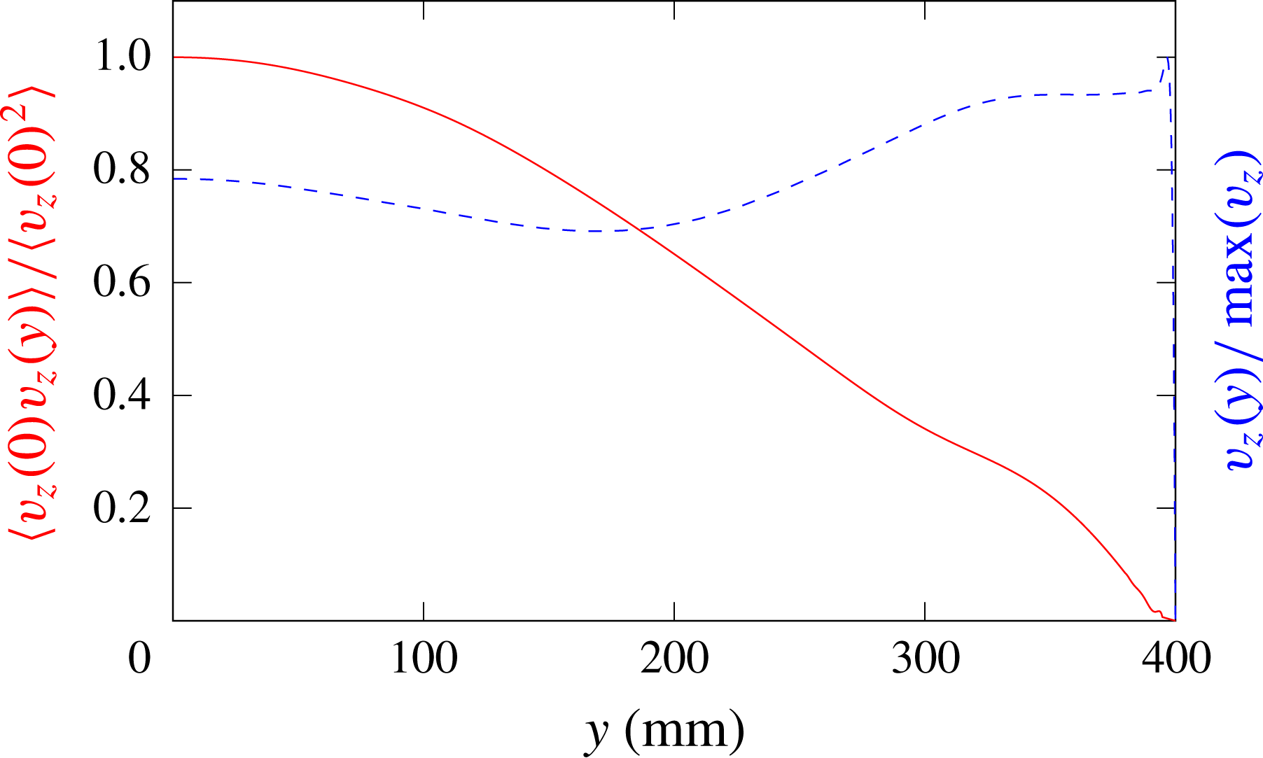
Figure 8 shows the correlation
 $\langle v_{z}(0,t)v_{z}(y,t)\rangle /\langle v_{z}(0,t)^{2}\rangle$
between the vertical velocity at the beginning of the probe line (located at the central vertical plane
 $y=0$
, coming through the middle of the wavemaker) and the vertical velocity at a different transverse location
 $y$
at the same line. Time averaging has been performed over 102 periods of the forcing oscillation. The value of the correlation decreases with the transverse coordinate. The dashed line shows the transverse distribution of the velocity amplitude
 $v_{z}(y)/\max (v_{z})$
along the same line, normalized by the maximum velocity at the probe line. These pictures as well as the analysis of 3D isosurfaces reveal that the velocity amplitude has a non-monotonic dependence on the transverse coordinate. It reaches the maximum close to the lateral wall before falling down to zero due to the no-slip boundary condition. The behaviour of the correlation coupled with the behaviour of the velocity amplitude allows us to conclude that there is also a phase shift between the wave motions at different transverse locations.
Correlation
 $\langle v_{z}(0,t)v_{z}(y,t)\rangle /\langle v_{z}(0,t)^{2}\rangle$
(solid red line) and normalized velocity
 $v_{z}(y)/\max (v_{z})$
(dashed blue line) as functions of the transverse coordinate
 $y$
for the same parameters as in figure 7.

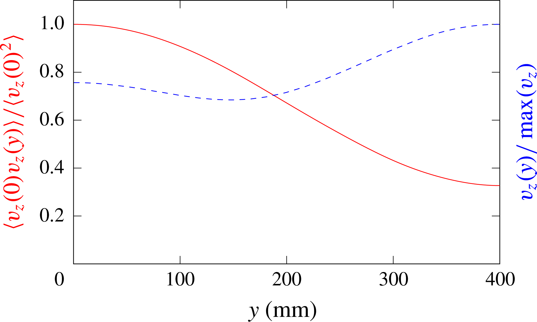
To isolate the effect of the wall friction on the lateral wall, we present in figure 9 the results of similar calculations performed for a stress-free boundary condition at the lateral wall. By comparing the results of simulations with the no-slip (figures 7 and 8) and stress-free boundary conditions (figure 9) at the lateral wall, we note that the latter case exhibits a more regular and smooth dependence of the calculated quantities on the transverse coordinate: in particular, there is no localized sharp maximum of the velocity amplitude close to the free-slip lateral wall. The shapes of the sharp maxima observed in calculations with the no-slip condition at the lateral wall (see figure 8) are reminiscent of the ‘cat ear’ velocity profiles calculated in Brouzet et al. (Reference Brouzet, Sibgatullin, Scolan, Ermanyuk and Dauxois2016b ) where such features were attributed to the effect of localized recirculating flows. Applying standard boundary layer theory as in Beckebanze et al. (Reference Beckebanze, Brouzet, Sibgatullin and Maas2018) should provide an elaborate description of the viscous dissipation in the interior shear layer, as well as at the rigid boundaries. Modification of the geometry and viscosity in calculations produce a variety of different amplitude and phase distributions, which will be described in a separate paper.
Same as figure 8 with stress-free, instead of no-slip, boundary conditions at lateral walls.

4 The canal-like geometry
4.1 Ray tracing prediction
The second experimental set-up is of particular interest since it echoes some in situ measurements. While internal waves have been measured close to the mouth of the Laurentian Channel, eastern Canada, they appear to be of very low intensity (Wang, Ingram & Mysak Reference Wang, Ingram and Mysak1991). This is surprising as internal wave dissipation in the ocean is known to be small, normally allowing internal waves to propagate thousands of kilometres before vanishing (Alford Reference Alford2003). Here this occurs even though internal tides are known to be generated at the land-locked head of the Channel (Cyr, Bourgault & Galbraith Reference Cyr, Bourgault and Galbraith2015). A possible explanation for this phenomenon could precisely be the refractive focusing mechanism investigated here, especially if tidal energy could now form attractors, as in figure 4, that are trapped on transverse planes. This is why we will study a model geometry of this physical situation, looking for the potential presence of these attractors.
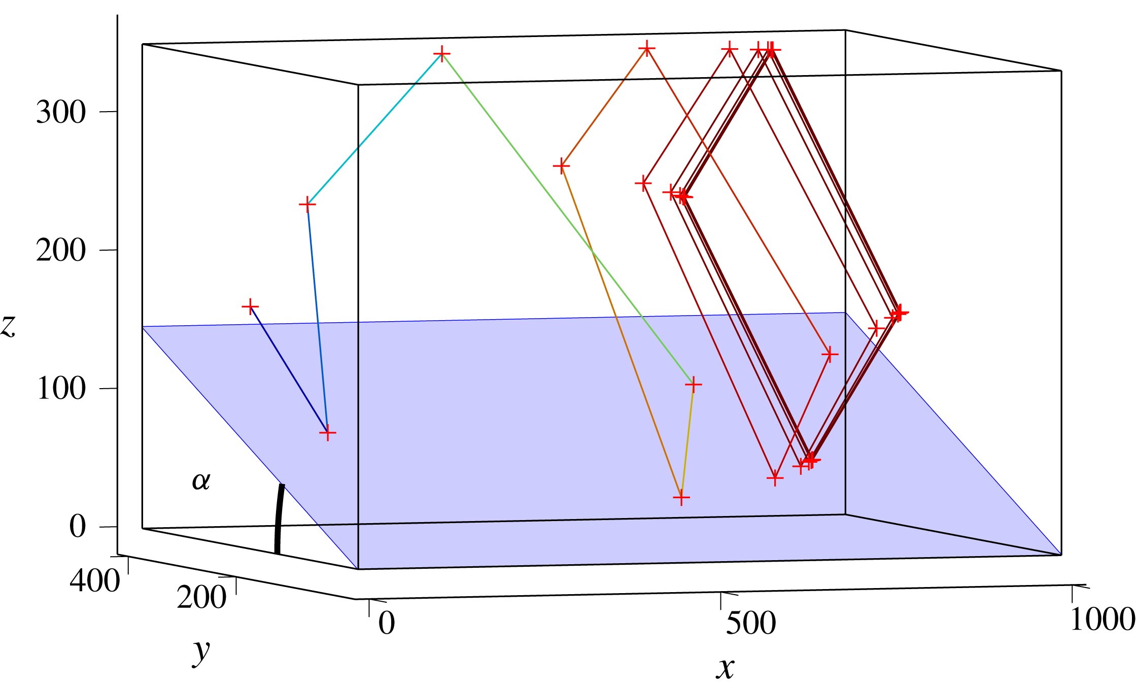
Trajectory of a single internal wave beam propagating in the canal-like geometry filled with a linearly stratified fluid. The beam is sent downwards (in the negative
 $z$
-direction) from the plane
 $x=0$
with
 $\unicode[STIX]{x1D719}_{0}=90^{\circ }$
(i.e. into the positive, along-tank
 $x$
-direction). Dimensions are in mm.

Figure 10 presents such a set-up for which an internal ray beam path leads to an attractor in a plane transverse to the along-slope, down-canal direction into which rays are initially launched. A sloping bottom is inserted in a parallelepiped tank. It makes an angle
 $\unicode[STIX]{x1D6FC}$
with the horizontal. Starting from an initial point on the wall
 $x=0$
, an internal wave beam of a given frequency
 $\unicode[STIX]{x1D714}$
launched with an angle
 $\unicode[STIX]{x1D719}_{0}=90^{\circ }$
will reflect several times on the different walls, as shown in figure 10. At each bounce off the inclined slope, the value of
 $\unicode[STIX]{x1D719}$
changes and converges to
 $0^{\circ }$
, i.e. onto a
 $yz$
-plane, transverse to the initial direction, which we call the focusing plane. In the remainder of this paper, we will index these focusing planes by their asymptotic
 $x$
-value, which we call
 $x_{\infty }$
. Moreover, as the transverse geometry of the canal has one inclined slope, it can lead to an attractor (Maas Reference Maas2005). One finds that, for a large range of angles
 $\unicode[STIX]{x1D6FC}$
, frequency ratios
 $\unicode[STIX]{x1D714}/N$
and ray launching positions, attractors can be created. In nearly all these cases, the ray will eventually not propagate downstream any longer (for exceptional ‘whispering gallery’ type waves that escape trapping, see Maas (Reference Maas2005) and Drijfhout & Maas (Reference Drijfhout and Maas2007)). Consequently, one can identify a zone of propagation of the internal wave ray, followed by a zone of trapping, and finally a zone without any internal waves.
A careful analysis shows that, for given values of
 $\unicode[STIX]{x1D6FC}$
and
 $\unicode[STIX]{x1D703}$
, the focusing plane depends on the initial angle
 $\unicode[STIX]{x1D719}_{0}$
with which the ray is launched and on its initial position
 $(x_{0},y_{0},z_{0})$
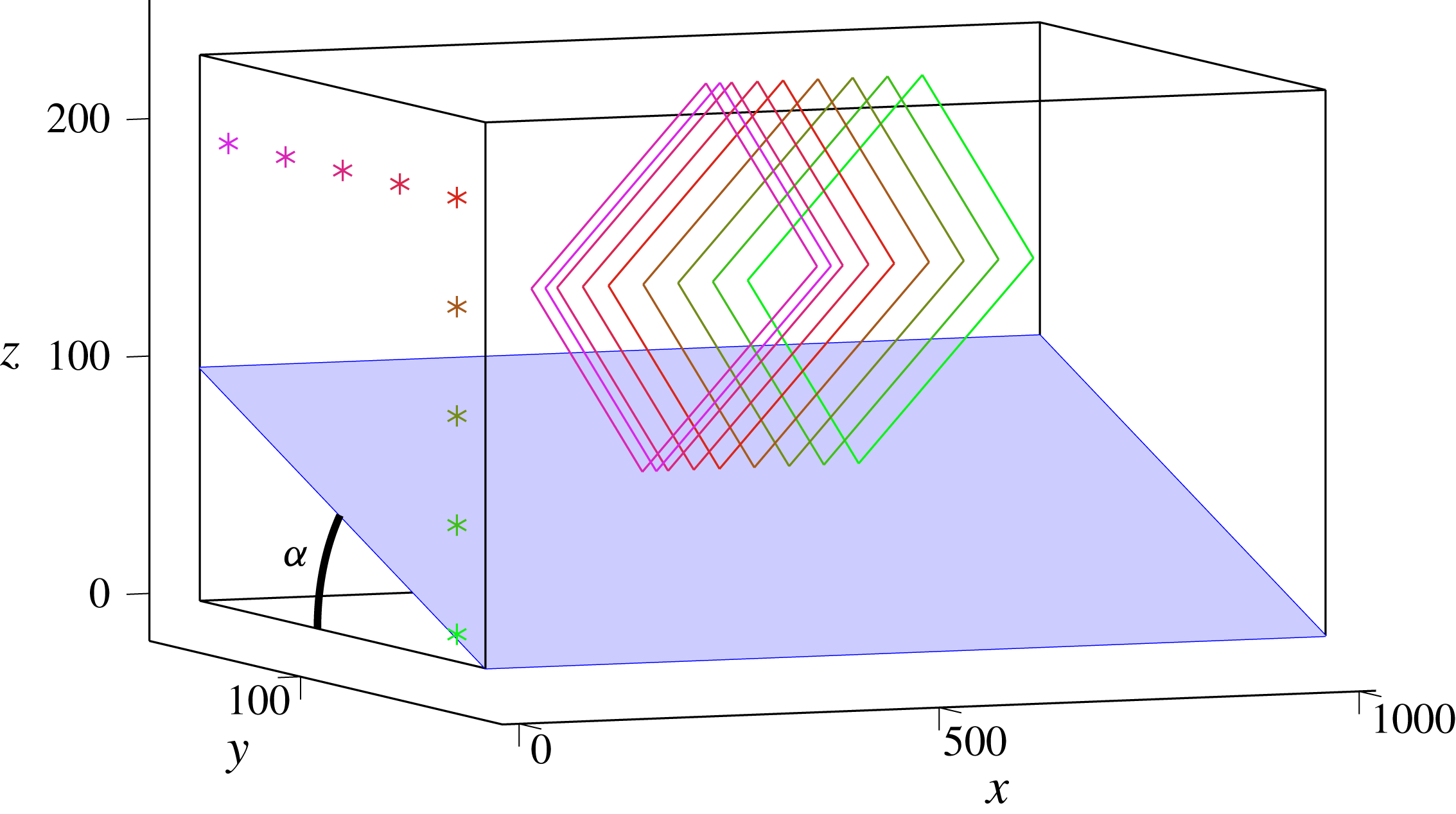
. To give an idea of the initial position dependence of
 $x_{\infty }$
, figure 11 presents the different steady paths created from several initial positions, all located in the same
 $x=0$
transverse plane. The initial positions are represented by the
 $\ast$
symbols while the steady paths correspond to the coloured lines. One can see that every point leads to a different attractor, each of them lying in a different transverse plane.
Final steady paths launched from different positions in the
 $x=0$
plane, represented by the different
 $\ast$
symbols. The rays are launched downwards with
 $\unicode[STIX]{x1D719}_{0}=90^{\circ }$
. The colour is the same for the initial point and the corresponding steady path. Dimensions are in mm.

In order to have an idea of where to expect the attractors, one can compute, for a given set of parameters (
 $\unicode[STIX]{x1D6FC}$
,
 $\unicode[STIX]{x1D703}$
,
 $\unicode[STIX]{x1D719}$
), the position map of the focusing plane as a function of
 $y_{0}$
and
 $z_{0}$
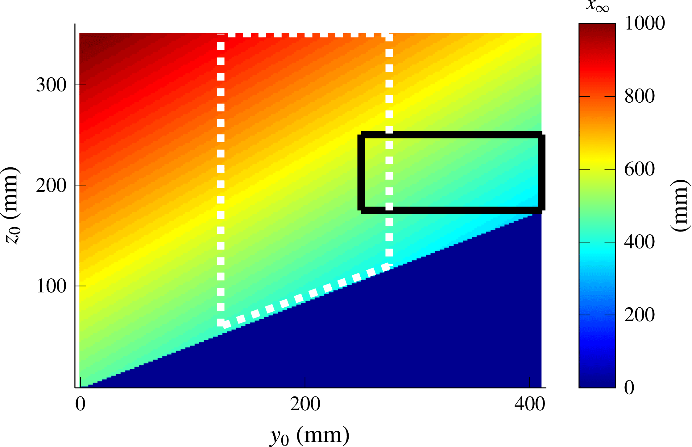
. This map presented in figure 12 is computed for a set of parameters used in the experiment described below. It emphasizes that, depending on the region of forcing, attractors can be created close to or far away from the generator. Please note already that, in the experiments, forcing of the fluid will be applied over an initial bounded
 $(y_{0},z_{0})$
-region. In doing so, one can thus expect to find attractors only in a given region of space.
For every initial point
 $(y_{0},z_{0})$
, the
 $x$
-position of the focusing plane is plotted. The parameters for this computation are
 $\unicode[STIX]{x1D6FC}=23^{\circ }$
,
 $\unicode[STIX]{x1D703}=32^{\circ }$
,
 $H=360$
mm,
 $L=1000$
mm and
 $W=410$
mm. The rays are launched downwards with
 $\unicode[STIX]{x1D719}_{0}=90^{\circ }$
. The solid black (respectively, dotted white) contour represents the region where the plane wave (respectively, mode 1) profile is forced. The blue triangle corresponds to the uninteresting region below the slope.

4.2 Experiments
The aim is to reproduce this refractive focusing predicted by ray tracing, using a tank of
 $1200~\text{mm}\times 410~\text{mm}\times 400~\text{mm}$
. The tank is filled up to 360 mm above the flat bottom and, due to the generator’s thickness, the slope is only 1000 mm long. We chose the origin,
 $x=0$
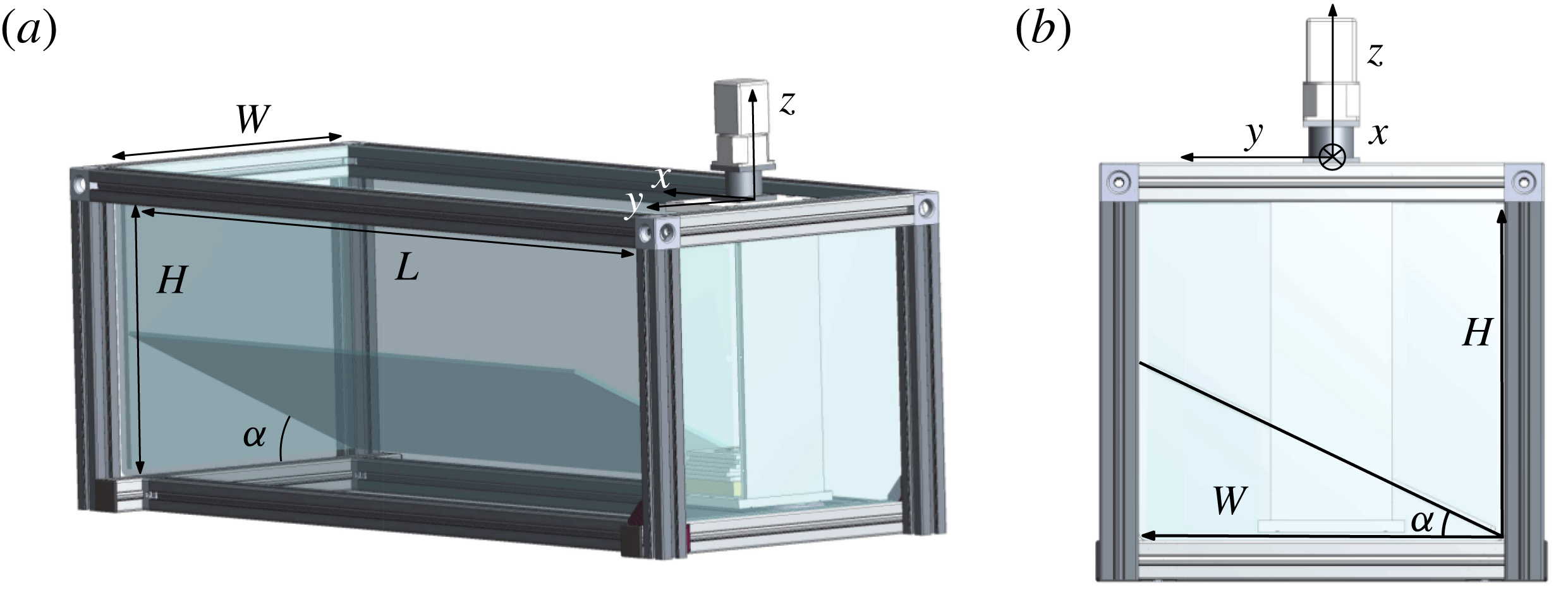
, at the edge of the wavemaker. Indeed, when experimentally studying narrow attractors, branches are not often easily distinguishable spatially. Another constraint is having a propagation angle sufficiently different from the slope angle, so that the first attractor branch will not be affected by viscous effects along the slope. These experimental difficulties greatly restrict the parameter space, leaving us few possibilities to obtain reliable data. The present set-up takes care of this issue by considering a tank that is less wide than the previous one, shown in figure 4. The transverse geometry is taken square-shaped, except for an additional slope of angle
 $\unicode[STIX]{x1D6FC}=23^{\circ }$
that is put at the bottom of the tank (see figure 13). Thus one may expect to create approximately square-shaped attractors that are easier to observe and to analyse.
The canal-like geometry: perspective (a) and side (b) views of the experimental set-up. The slope and the wave generator are visible. The parameters used for the experiment are
 $H=360$
mm,
 $L=1000$
mm,
 $W=410$
mm and
 $\unicode[STIX]{x1D6FC}=23^{\circ }$
.

For this geometry, two types of forcing were used.
(i) A mode 1 profile
$\unicode[STIX]{x1D701}(z,t)=a\sin (\unicode[STIX]{x1D714}t)\cos (\unicode[STIX]{x03C0}z/H)$
, limited to the dashed white region in figure 12 as previously, where
$H$
is the total height of the fluid,
$a$
the amplitude of motion of the cams and
$\unicode[STIX]{x1D714}$
the frequency of the forcing. This modal type of forcing can be interpreted as sending of internal wave beams in both upward as well as downward directions. Corresponding results are shown in figures 14 and 15.(ii) A plane-wave profile
$\unicode[STIX]{x1D701}(z,t)=a\sin (\unicode[STIX]{x1D714}t+2\unicode[STIX]{x03C0}z/\unicode[STIX]{x1D706})$
, limited to the black rectangular region in figure 12 in which the wavelength
$\unicode[STIX]{x1D706}$
and the numbers of wavelengths can be chosen. We choose to force the fluid with only one wavelength. The upward phase propagation, adopted here, implies that an inclined, downward-directed internal wave beam is generated. Corresponding results are shown in figure 16.





For this experiment, a laser sheet is created above the tank that illuminates a transverse
 $yz$
-section of the tank. The laser sheet can be translated to obtain different vertical slices of the tank. As before, we use the PIV method to obtain the velocity field. As previously, a Hilbert filtering is eventually used to filter the velocity field and to get rid of the noise.
In order to quantify the presence of the attractors and then conclude on the focusing effect predicted, we first force the fluid with a mode 1 with
 $a=0.5~\text{mm}$
, the generator being put at the middle of the tank width. As we can see in figure 12, with this forcing applied to the region inside the dashed white rectangle, a large band of
 $150~\text{mm}\times 300~\text{mm}$
in (
 $y_{0},z_{0}$
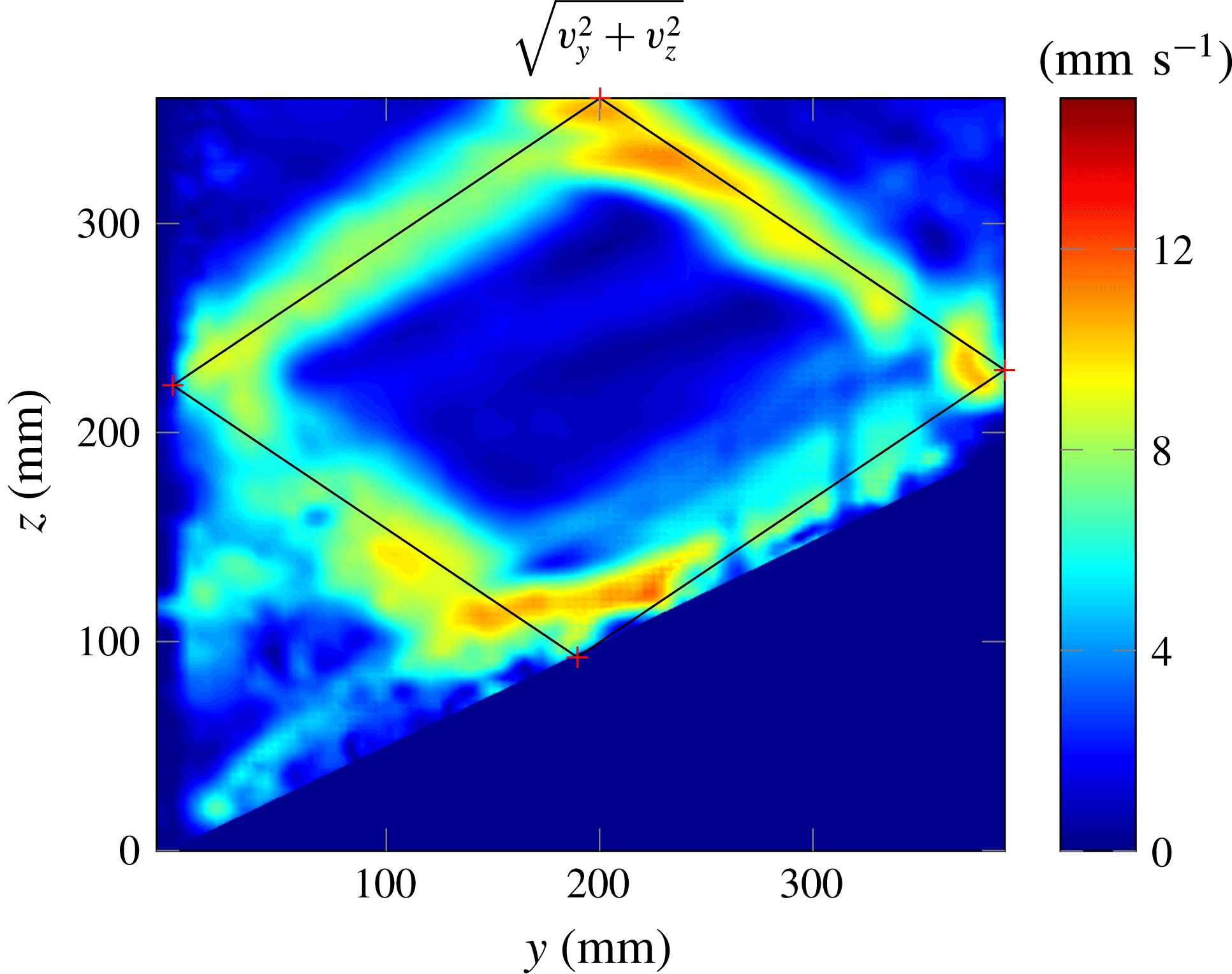
) is excited. One can thus expect that such a forcing will create attractors approximately everywhere in the tank. Experimentally, we do find attractor-like velocity fields over the whole length of the tank. Figure 14 presents an example of the velocity field obtained for a slice where the amplitude is large: one clearly sees an attractor. The ray tracing prediction, calculated for the same parameters, has been superimposed on the experimental image, emphasizing the very good agreement.
Filtered velocity field amplitude
 $(v_{y}^{2}+v_{z}^{2})^{1/2}$
at the slice
 $x=700$
mm. The ray tracing prediction is superimposed. The experimental parameters are
 $\unicode[STIX]{x1D714}=0.51~\text{rad}~\text{s}^{-1}$
,
 $N=1.0~\text{rad}~\text{s}^{-1}$
and those of figure 13.

To be quantitative and exhibit an experimental proof of the focusing of the energy in a transverse plane, we look at the wave propagation angles precisely in this transverse plane. Indeed, PIV in a transverse laser sheet only measures the projection of the real velocity field in the laser sheet since the velocity perpendicular to the sheet (here,
 $v_{x}$
, the velocity along
 $x$
) is not observed. If
 $v_{x}$
is small compared to the velocities in the other directions, then the propagation angle should follow the dispersion relation of internal waves
 $\unicode[STIX]{x1D714}=\pm N\sin \unicode[STIX]{x1D703}$
.
In order to obtain the angles of propagation of the projected velocity field, we proceed in several steps that were already proposed in Brouzet et al. (Reference Brouzet, Ermanyuk, Joubaud, Sibgatullin and Dauxois2016a
). First, we filter the velocity field in
 $\unicode[STIX]{x1D714}$
using the Hilbert transform. Second, we perform the Fourier transform on
 $v_{y}$
and
 $v_{z}$
, obtaining then the energy as a function of
 $k_{y}$
and
 $k_{z}$
, two components of the wavevectors. We then interpolate
 $E(k_{y},k_{z})$
as a function of the perpendicular wavenumber
 $k_{\bot }=(k_{y}^{2}+k_{z}^{2})^{1/2}$
and of the projected angle of propagation
 $\unicode[STIX]{x1D703}_{\bot }=\text{arcsin}(k_{z}/k_{\bot })$
to obtain
 $E(k_{\bot },\unicode[STIX]{x1D703}_{\bot })$
. Integrating finally over all values of
 $k_{\bot }$
, we get the energy density
 $E(\unicode[STIX]{x1D703}_{\bot })$
.
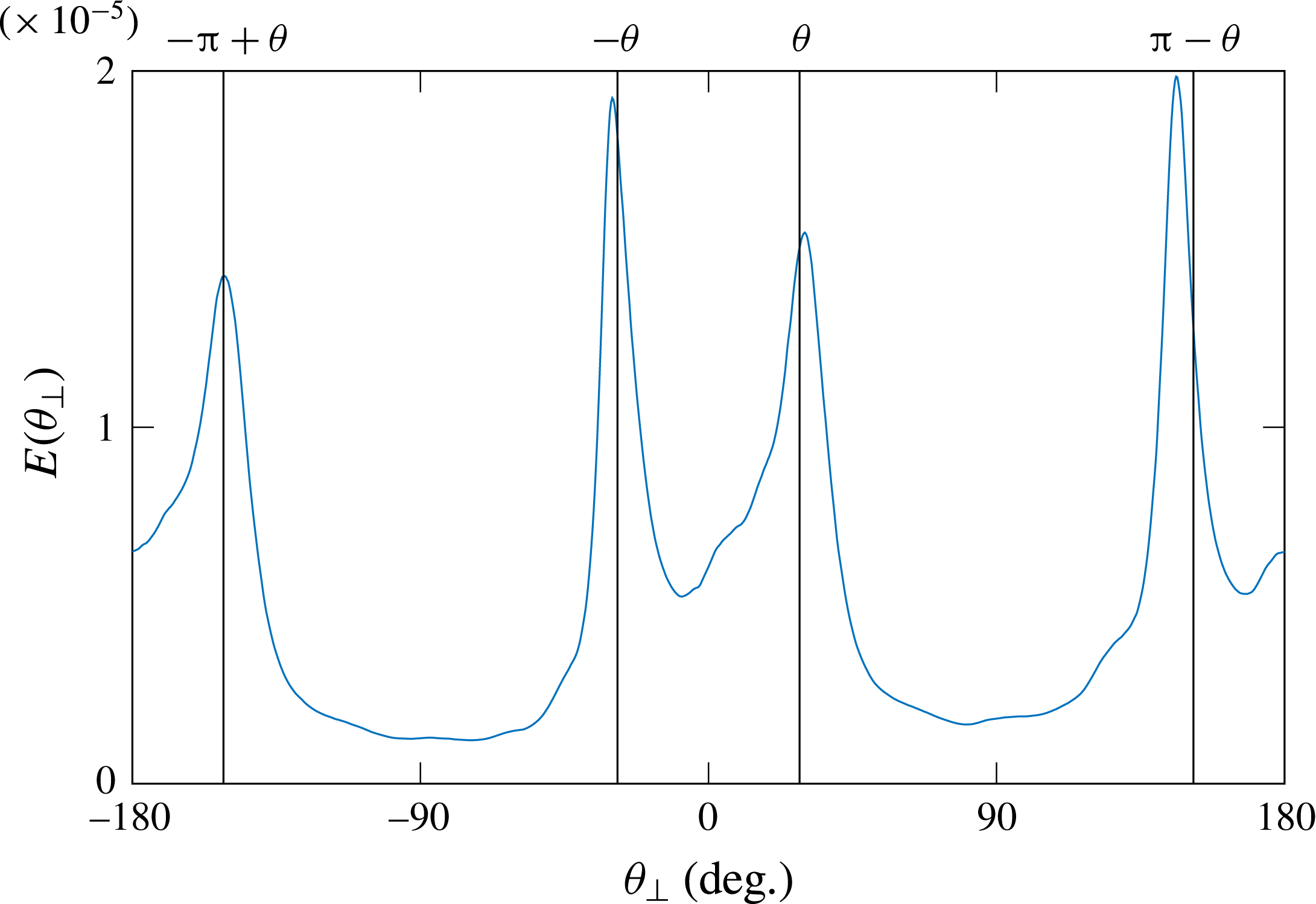
Angular repartition of the energy density
 $E(\unicode[STIX]{x1D703}_{\bot })$
for the filtered velocity field of the figure 14. The four black vertical lines represent the four
 $\unicode[STIX]{x1D703}$
values given by the dispersion relation determined by the forcing frequency.

When applying this treatment to the velocity field shown in figure 14, we obtain the
 $E(\unicode[STIX]{x1D703})$
repartition shown in figure 15. The four black vertical lines represent the four
 $\unicode[STIX]{x1D703}$
-values compatible with the dispersion relation considering the experimental forcing frequency
 $\unicode[STIX]{x1D714}$
. One can see that the four peaks, representing the four branches of the attractor, fall on the four peaks theoretically expected. So, as predicted by ray tracing, the focusing effect is taking place here.
To highlight the effect of energy trapping, due to this focusing enhanced in the ray tracing calculations, we now rely on a forcing with a plane wave. The goal is to create an attractor only in a given region of the canal to see, first, propagating energy near the generator, then attractors in the middle of the tank, and finally very low wave propagation beyond, due to the trapping of the waves. We choose a rather large wavelength,
 $\unicode[STIX]{x1D706}=75~\text{mm}$
, to limit the damping, but only one wavelength, to create attractors in a limited region only. The forcing amplitude is
 $a=0.5~\text{mm}$
. The region of the forcing is shown in figure 12 by the region inside the black solid contour.
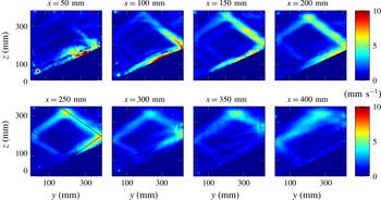
Filtered velocity amplitude
 $(v_{y}^{2}+v_{z}^{2})^{1/2}$
for different slices of the tank. The experimental parameters are
 $\unicode[STIX]{x1D714}=0.45~\text{rad}~\text{s}^{-1}$
,
 $N=0.89~\text{rad}~\text{s}^{-1}$
and those of figure 13. For
 $x=250~\text{mm}$
, the ray tracing prediction is superimposed.

Figure 16 shows nicely the successful experiment. At the beginning (
 $x=50$
–100 mm), one can see a shapeless velocity field; further downstream (
 $x=150$
–300 mm), the attractor is created and especially visible in the two most energetic branches; beyond the focusing zone, the energy is very low. Although the ray tracing predicted the attractor region around
 $x=400$
mm, it appears to be located closer to
 $x=250$
mm. The difference can be explained by the strong sensitivity of figure 12 on the parameters of the experiment.
Similarly to what has been performed for the reference case presented in figure 15, to get a more quantitative picture and show the energy focusing in a small region of the canal, it is useful to plot the position of the peaks of
 $E(\unicode[STIX]{x1D703}_{\bot })$
obtained for different slices. In this case, the procedure needs some care. For the first slices, waves propagate mainly through the observation planes. The velocity field produced by PIV is therefore not representative of the real 3D velocity field, hence the peaks are not clearly defined. One first step is to filter the velocity field in the
 $k_{\bot }$
space. Using the Hilbert method again, one can filter the velocity field for (
 $k_{y},k_{z}>0$
), (
 $k_{z}<0<k_{y}$
), (
 $k_{y}<0<k_{z}$
) and (
 $k_{y},k_{z}<0$
), giving separately the four branches of the attractor. This procedure has proven its utility for the four branches of the St Andrew’s cross (Mercier et al.
Reference Mercier, Garnier and Dauxois2008) or for 2D attractors (Brouzet et al.
Reference Brouzet, Sibgatullin, Ermanyuk, Joubaud and Dauxois2017). For each branch, one can moreover plot the angular repartition of the energy.
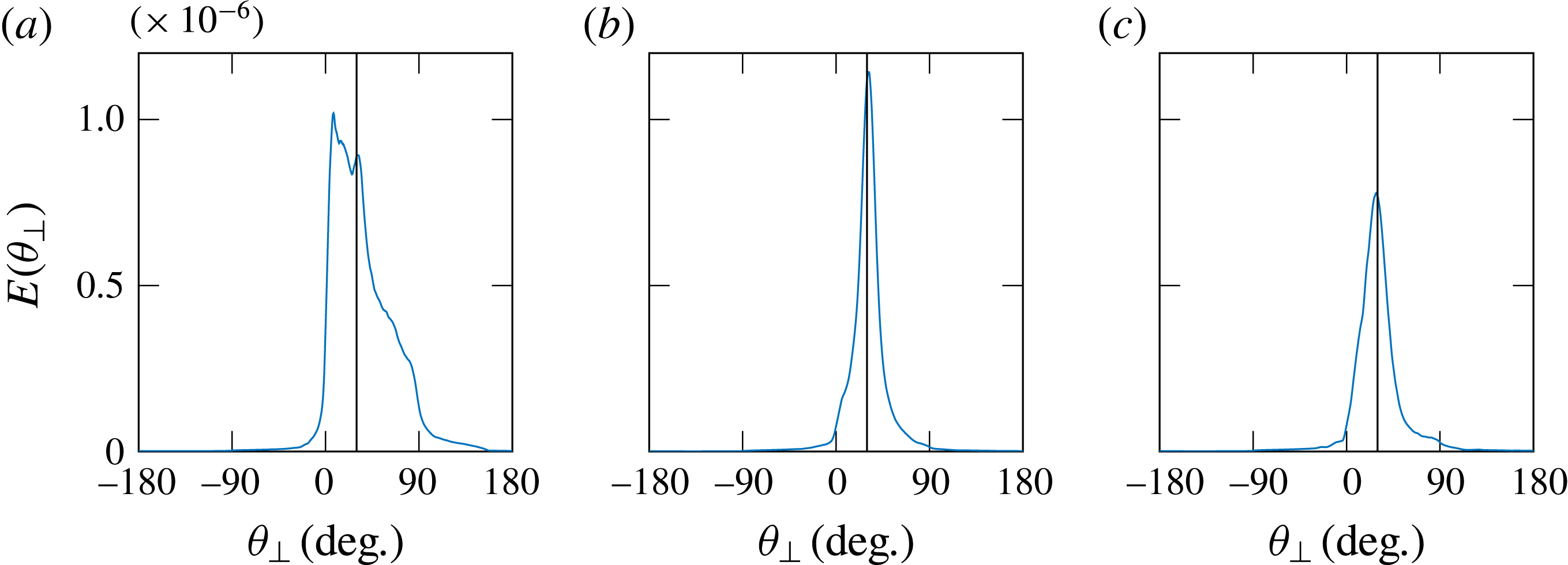
Angular repartition of energy for branch 3 corresponding to (
 $k_{y}>0$
,
 $k_{z}>0$
) for three slices:
 $x=50$
mm (a),
 $x=250$
mm (b) and
 $x=450$
mm (c).

We thus study the positions of the peaks and their shape along the longitudinal
 $x$
-direction. For instance, figure 17 presents the angular repartition of the energy for
 $k_{y}>0$
and
 $k_{z}>0$
, i.e. in branch 3, counting anticlockwise from the attractor’s slope reflection, three different slices corresponding to three different
 $x$
-positions. At the beginning and therefore close to the injection (
 $x=50$
mm, figure 17
a), the energy is not focused on a single peak, and not even centred on the expected angle, represented by the solid vertical line: the wave is still propagating transversely to the observation slice. Further downstream in the canal (
 $x=250$
mm, figure 17
b), the energy is almost centred along one single peak and its position corresponds to the angle given by the dispersion relation: focusing has occurred and the waves are almost trapped in the observation slice. Even further downstream (
 $x=450$
mm, figure 17
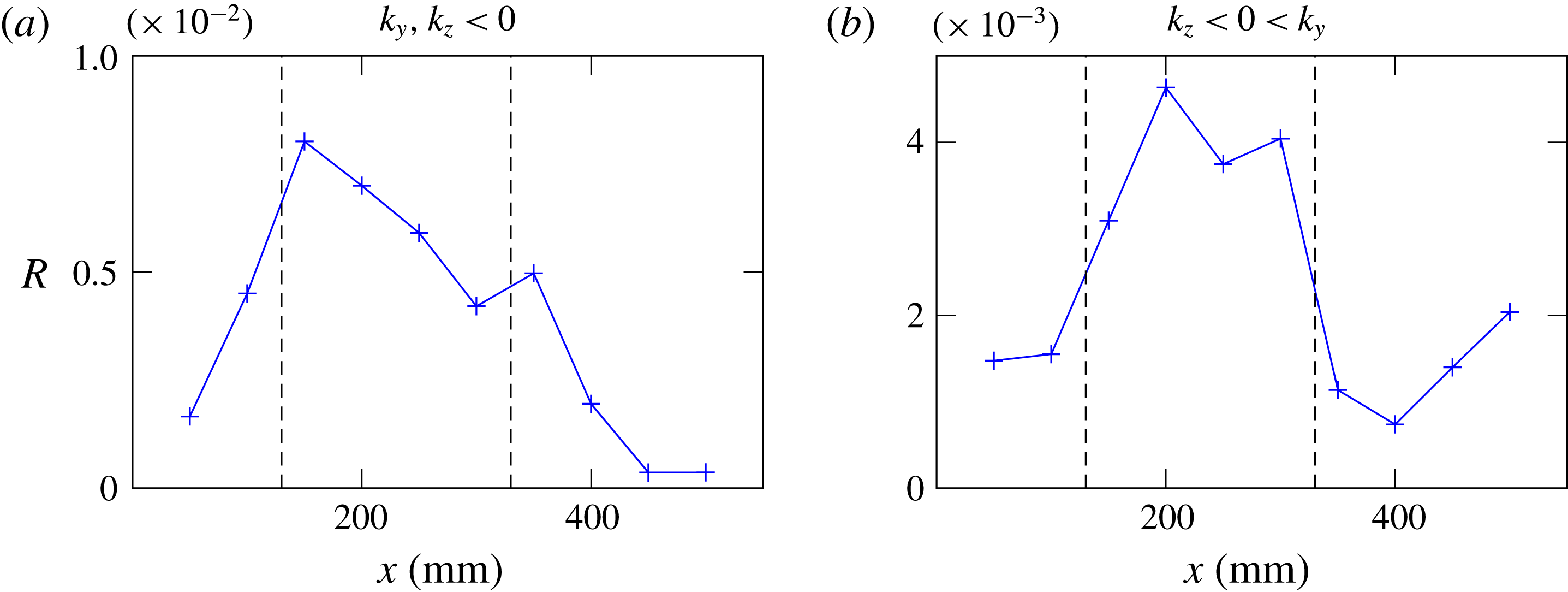
c), the waves are still almost in the transverse plane, but the energy has significantly decreased, as the trapping occurred upstream. Of course, damping also plays a role to explain this decrease. That is why, to emphasize the focusing, one may track the position of each of the four peaks, for all slices. However, as emphasized by the previous example, the peak position is not always the relevant quantity. The ratio of the peak amplitude to the total transverse slice energy
 $$\begin{eqnarray}R={\displaystyle \frac{\max (E(\unicode[STIX]{x1D703}_{\bot }))}{\displaystyle \int _{slice}(v_{y}^{2}+v_{z}^{2})\,\text{d}y\,\text{d}z}}\end{eqnarray}$$
is a more appropriate indicator. If this quantity is relatively large, it indicates that the energy is well focused around the main peak and therefore looking at the peak position makes sense. On the contrary, if this quantity is low, one cannot clearly define a single direction of propagation in this region of the
 $k$
-space and at this slice. The ratio (4.1) can be calculated for all four branches of the attractor, but we chose to focus only on the two most energetic ones, obtained by filtering
 $k_{\bot }$
for branch 2 (
 $k_{y},k_{z}<0$
) and for branch 1 (
 $k_{z}<0<k_{y}$
). Figure 18 presents the value of
 $R$
for these two branches, for all slices.
Ratio
 $R$
of the peak amplitude divided by the total energy of a slice. (a,b) Correspond to the two most energetic branches of the attractor, branch 2 (a) and branch 1 (b). The dashed lines represent the zone where
 $R>\max (R)/2$
for (b).

Taking the most energetic branch (figure 18
b), one can define a zone of confidence by the region for which
 $R>\max (R)/2$
. This region, emphasized with the vertical dashed lines in figure 18, is approximately located between
 $x=130$
mm and
 $x=320$
mm.
This quantity is not a proof of the focusing in itself but gives a good indication at which
 $x$
-position along the canal it is relevant to study the peak positions in the
 $(E,\unicode[STIX]{x1D703})$
diagram. For these two branches, one can rely on the
 $E(\unicode[STIX]{x1D703}_{\bot })$
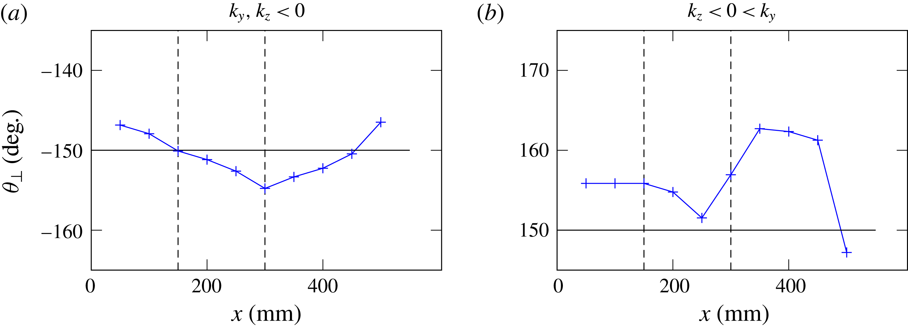
peak position values if the slice is taken between the dashed lines. In this area, one can expect a good estimate of the transverse angle of propagation
 $\unicode[STIX]{x1D703}_{\bot }$
. In figure 19, the peak position is plotted for all the slices, for the two branches. We add moreover in each plot a horizontal line representing the expected propagation angle and two vertical dotted lines to show the confidence zone. For
 $x$
-values in this zone, one can see that the propagation angles correspond to the expected ones, confirming that, in these slices, the propagation is almost totally transverse: trapping occurred because of the focusing effect.
Peak position for all slices, for the two most energetic branches. The vertical dashed lines delimit the region in which the energy is significantly focused on a single
 $\unicode[STIX]{x1D703}$
-value, so where looking at the peak position makes sense. The horizontal black line shows the expected value of the propagation angle.

The ratio
 $R$
combined with the peak position for many
 $yz$
-slices allows us to conclude that there is indeed a region between approximately
 $x=150$
mm and
 $x=300$
mm where propagation of most of the energy is totally transverse. As predicted by ray tracing, the refractive focusing mechanism is now experimentally confirmed.
5 Conclusion
We studied experimentally two simple 3D geometries. The first one is slightly different from a classical 2D study case for (1,1)-attractors. The difference lays in the forcing, which is non-uniform, since we are forcing only over a 150 mm wide lateral interval in a 800 mm wide tank. The ray tracing in this geometry shows that, if the rays are sent with a small angle with respect to the bottom-normal direction, they spread everywhere throughout the tank, before ending up in a plane oriented normal to the sloping bottom, always forming attractors. This prediction was then confirmed experimentally. We showed first that the attractor velocity field is nearly identical everywhere in the tank even though forcing only occurs in the middle of the tank. In a subsequent experiment, we showed that attractors are created approximately everywhere almost simultaneously. Moreover, the energy was roughly uniformly spread throughout the tank, giving two strong arguments in favour of the proposed mechanism of generation by refractive trapping. Complementary numerical experiments also confirmed the results, revealed a phase shifting in the transverse direction and provided in addition a very interesting confirmation of the role of boundary conditions. In particular, they emphasize the stronger localized response near lateral walls when using a no-slip instead of stress-free boundary condition.
In the second experiment, the geometry of the tank is closer to a canal having a sloping bottom. The forcing is applied in the along-slope, longitudinal direction of the canal. The ray tracing and the experimental data showed unambiguously that the propagation ends up transversely to the canal. Experimentally, we proved the refractive focusing by looking at the angular repartition of the energy. We showed, indeed, that, once focused, waves propagate at the angles expected by the dispersion relation. We also showed that this focusing can significantly reduce the energy at the end of the canal, since waves are rapidly trapped in transverse planes. This may provide a tentative explanation for in situ measurements of the Laurentian Channel, which show measurements of unexpectedly low internal wave energy far away from the channel head, as yet unexplained (Wang et al. Reference Wang, Ingram and Mysak1991). Subsequent observations, along one side of this Channel, do show evidence of internal tides. These appear to be forced at the nearby located transverse sill at the head of the Laurentian Channel, and while initially expected to propagate down-channel, they appear to be responsible for observed transverse internal tidal motions (Cyr et al. Reference Cyr, Bourgault and Galbraith2015), such as expected from the refractive trapping mechanism.
This work shows the importance of the refractive focusing effect when considering 3D reflection of internal gravity waves. In both cases studied in this paper, the structure eventually created in the transverse planes is a 2D-like attractor. The parameter space diagrams suggest that attractors are indeed generic for these geometries. It is likely that there is a direct link between the focusing and the existence of attractors. Work along this line is in progress.
Acknowledgements
This work was supported by the LABEX iMUST (ANR-10-LABX-0064) of Université de Lyon, within the programme ‘Investissements d’Avenir’ (ANR-11-IDEX-0007), operated by the French National Research Agency (ANR). This work has been supported by the ANR through grant ANR-17-CE30-0003 (DisET). This work has achieved thanks to the resources of PSMN from ENS de Lyon. Direct numerical simulations were performed on supercomputer ‘Lomonosov’ of Moscow State University.