


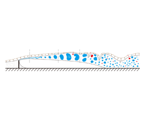

1. Introduction
In many turbulent flows, such as jets, mixing layers and turbulent boundary layers, the flow field can be divided into two distinct regions: the turbulent region characterized by high-vorticity fluids and the non-turbulent region where the flow is theoretically irrotational (Corrsin & Kistler Reference Corrsin and Kistler1955). These two regions are separated by a thin and strongly convoluted interface known as the turbulent/non-turbulent interface (TNTI), across which turbulent entrainment occurs (da Silva et al. Reference da Silva, Hunt, Eames and Westerweel2014a). Entrainment refers to the process where irrotational fluids become part of the turbulent region, which is responsible for the transfer of mass, momentum and energy between the turbulent flow and the adjacent non-turbulent flow. In view of its importance in the understanding of turbulent mixing, extensive efforts have been dedicated to identifying, quantifying and modelling entrainment in previous studies (Holzner & Luthi Reference Holzner and Luthi2011; Wolf et al. Reference Wolf, Lüthi, Holzner, Krug, Kinzelbach and Tsinober2013; Jahanbakhshi & Madnia Reference Jahanbakhshi and Madnia2016; Mistry et al. Reference Mistry, Philip, Dawson and Marusic2016; Jahanbakhshi Reference Jahanbakhshi2021; Long, Wang & Pan Reference Long, Wang and Pan2022a; Xu, Long & Wang Reference Xu, Long and Wang2023; Zhang, Watanabe & Nagata Reference Zhang, Watanabe and Nagata2023).
It is generally agreed that the entrainment process consists of two mechanisms: nibbling and engulfment (da Silva et al. Reference da Silva, Hunt, Eames and Westerweel2014a). Nibbling refers to the mechanism by which the fluids near the TNTI acquire vorticity due to vorticity diffusion and becomes part of the turbulent region, and engulfment refers to the process in which the irrotational fluids are drawn directly into the turbulent region before they acquire vorticity (Mathew & Basu Reference Mathew and Basu2002; Taveira et al. Reference Taveira, Diogo, Lopes and da Silva2013; Chauhan, Philip & Marusic Reference Chauhan, Philip and Marusic2014; da Silva et al. Reference da Silva, Hunt, Eames and Westerweel2014a; Jahanbakhshi & Madnia Reference Jahanbakhshi and Madnia2016). Nibbling occurs continuously on almost the entire TNTI and is usually considered to be related to the outward spreading of small-scale vortices in the vicinity of the TNTI (Mathew & Basu Reference Mathew and Basu2002; Westerweel et al. Reference Westerweel, Fukushima, Pedersen and Hunt2005). In recent studies, the nibbling mechanism is generally quantified by the local entrainment velocity, defined as the velocity of the TNTI relative to the flow, which is of Kolmogorov scale and dominated by the viscous component (Holzner & Luthi Reference Holzner and Luthi2011; Jahanbakhshi & Madnia Reference Jahanbakhshi and Madnia2016; Mistry et al. Reference Mistry, Philip, Dawson and Marusic2016; Long et al. Reference Long, Wang and Pan2022a). Engulfment takes place occasionally and is mostly caused by the motions of large-scale eddies, usually forming low-vorticity pockets (also known as bubbles) in the turbulent region (Mathew & Basu Reference Mathew and Basu2002; Taveira et al. Reference Taveira, Diogo, Lopes and da Silva2013; Jahanbakhshi & Madnia Reference Jahanbakhshi and Madnia2016). As large-scale motions exhibit some distinct characteristics in diverse flows, the contribution of nibbling and engulfment to total entrainment might vary in each flow (Philip & Marusic Reference Philip and Marusic2012). For example, it was reported that engulfment is the dominant mechanism in wakes (Bisset, Hunt & Rogers Reference Bisset, Hunt and Rogers2002; Hickey, Hussain & Wu Reference Hickey, Hussain and Wu2013), while nibbling plays the main role in the entrainment process in jets and turbulent boundary layers (Mathew & Basu Reference Mathew and Basu2002; Westerweel et al. Reference Westerweel, Fukushima, Pedersen and Hunt2005; Borrell and Jiménez Reference Borrell and Jiménez2016; Jahanbakhshi & Madnia Reference Jahanbakhshi and Madnia2016; Long et al. Reference Long, Wang and Pan2022a; Xu et al. Reference Xu, Long and Wang2023). In view of this fact, it is necessary to discuss the issue of whether nibbling or engulfment contributes more to the entrainment process depending on the specific flow type being considered.
To better understand the mechanisms of entrainment, considerable attention has been devoted to investigating the influence of turbulent coherent structures on entrainment. It was once reported that entrainment is mostly controlled by small-scale motions (Westerweel et al. Reference Westerweel, Fukushima, Pedersen and Hunt2005, Reference Westerweel, Fukushima, Pedersen and Hunt2009). The local entrainment velocity is modulated by the nearby Taylor microscale vortex (da Silva et al. Reference da Silva, Hunt, Eames and Westerweel2014a; Mistry, Philip & Dawson Reference Mistry, Philip and Dawson2019; Neamtu-Halic et al. Reference Neamtu-Halic, Krug, Mollicone, van Reeuwijk, Haller and Holzner2020), and statistically, the dominant length scale of TNTI normal velocity is the Taylor microscale (Balamurugan et al. Reference Balamurugan, Rodda, Philip and Mandal2020). By examining a model where an artificial small-scale eddy is positioned near the TNTI, Watanabe et al. (Reference Watanabe, Jaulino, Taveira, da Silva, Nagata and Sakai2017) demonstrated that details of entrainment movements are governed by small-scale eddies.
However, since the interaction between scales has been demonstrated to exist at modest Reynolds numbers by recent works (Buxton Reference Buxton2015; Fiscaletti et al. Reference Fiscaletti, Attili, Bisetti and Elsinga2016a,Reference Fiscaletti, Elsinga, Attili, Bisetti and Buxtonb), it seems inappropriate to ignore the contribution of large-scale motions in all cases. In fact, there are many works that emphasized the importance of large-scale motions for turbulent entrainment. Detailed multiscale analyses by Philip et al. (Reference Philip, Meneveau, de Silva and Marusic2014) and Mistry et al. (Reference Mistry, Philip, Dawson and Marusic2016) indicated that although the tortuosity of the TNTI and the local entrainment velocity vary in different scales, the total entrainment flux is independent of the scale. Philip et al. (Reference Philip, Meneveau, de Silva and Marusic2014) suggested that viscous effects at the smallest scales provide the physical mechanism ultimately responsible for entrainment, while the overall rate of entrainment is determined by the large-scale transport due to the energy-containing eddies. In addition, Cimarelli & Boga (Reference Cimarelli and Boga2021) conducted a numerical study where the large-scale and small-scale velocity fields were numerically separated and evolved independently. They found that entrainment is more intensive in the large-scale velocity field. Long et al. (Reference Long, Wang and Pan2022a) studied the modulations of large-scale motions on entrainment in the turbulent boundary layer. They indicated that high-speed large-scale motions enhance the engulfment by the sweep flow, whereas low-speed large-scale motions induce stronger instantaneous nibbling. Nonetheless, the integral nibbling flux is larger above high-speed motions due to the more distorted TNTI induced by high-speed large-scale motions. Moreover, the Reynolds number dependence of entrainment in the turbulent boundary layer was investigated in a recent study conducted by Zhang et al. (Reference Zhang, Watanabe and Nagata2023). The probability density functions (PDFs) of the local entrainment velocity agree well with each other for high Reynolds numbers when the local entrainment velocity is normalized by the friction velocity. They attributed this variation to the diminution of the direct wall effects on the small-scale motions and the prominence of the large-scale motions with the increase of the Reynolds number.
Most previous researches have been limited to the fully developed canonical flows such as jets, wakes, mixing layers and turbulent boundary layers. In contrast, only a few studies have focused on entrainment in more complex flows (Zhang, Rival & Wu Reference Zhang, Rival and Wu2021; Long, Wang & Wang Reference Long, Wang and Wang2022b) or developing flows (Philip et al. Reference Philip, Bermejo-Moreno, Chung and MARUSIC2015; Wu, Wallace & Hickey Reference Wu, Wallace and Hickey2019). Zhang et al. (Reference Zhang, Rival and Wu2021) studied the TNTI properties in the airfoil flow where separation bubbles, transition, turbulent boundary-layer separation and asymmetric wakes coexist in the complex spatially developing flow. They reported the propensity for local entrainment across the cross-streamwise and leading edges as well as the relatively flat surfaces of the TNTI after the transition, which resembled the behaviour observed in jets (Mistry et al. Reference Mistry, Philip and Dawson2019) and wakes (Philip et al. Reference Philip, Bermejo-Moreno, Chung and MARUSIC2015). However, in the early transitional stage, entrainment is not strongly influenced by the geometric properties of the TNTI. Long et al. (Reference Long, Wang and Wang2022b) explored the evolution of the TNTI above the main element of a multi-element airfoil. They indicated that the local entrainment flux increases along the streamwise direction, suggesting that the increase in tortuosity of the TNTI has a greater effect on entrainment than the decrease of the vorticity gradient in the transition.
Although many detailed researches have focused on turbulent entrainment, the evolution of entrainment and the effect of flow structures on entrainment in the transition process is not clear yet. In the present work we focuse on turbulent entrainment in the transition of the separated and reattaching flow induced by a fixed fence in the flat-plate boundary layer. Preliminary study has shown that the properties of the TNTI evolve significantly accompanied with the flow evolution from the separated shear layer, transition, reattachment and finally to the turbulent boundary layer (Li, Long & Wang Reference Li, Long and Wang2022). Whereas, the characteristics of turbulent entrainment in the transition are still unknown and intriguing. In addition, the separated and reattaching turbulent flows, which generally enhance the turbulent mixing, are also ubiquitous and important flows in nature and engineering. From the perspective of the TNTI, the studies on entrainment help to improve our understanding of the turbulent mixing. Therefore, the main objective of the present work is to study the evolution of turbulent entrainment and the effect of vortex structure on entrainment in the separated and reattaching flow.
This paper is organized as follows. The experimental equipment, parameters and the interface detection method are described in § 2. The mean characteristics of the separated and reattaching flow and the dynamics of the shedding vortex are illustrated in § 3. The streamwise variations of entrainment and the effects of vortex structures on entrainment are studied in § 4. Finally, this paper is summarized in § 5.
2. Experimental methods
2.1. Experimental set-up
To analyse the entrainment properties, a time-resolved particle image velocimetry (PIV) experiment was conducted in the low-speed water channel at Beihang University. Actually, the experimental set-up was similar to that in our preliminary study (Li et al. Reference Li, Long and Wang2022) except for the PIV system. Nevertheless, essential parameters are described here again to ensure the integrity of this work and to make it convenient for the reader. As illustrated in figure 1(a), a flat and smooth acrylic plate was vertically fixed in the centre of the 3 m long, 60 cm wide channel. The length, width and thickness of the plate were 200, 50 and 1.5 cm, respectively, and the free surface of water just submerged the top of the plate. The ratio of the plate width to the half-width of the flume was 3.33, and the flume was quite wide in the spanwise direction. An elliptic leading edge with the aspect ratio of  $5:1$ was utilized to avoid flow separation from the leading edge of the plate.
(a) Sketch of the experimental set-up. (b) Mean profile of the streamwise velocity for the laminar boundary layer.

To ensure that a stable incoming flow was guaranteed by this experimental set-up, the unperturbed boundary layer on the smooth surface of the plate was examined before installing the fence. Figure 1(b) shows the mean profile of the streamwise velocity at the streamwise location where the fence was expected to be installed. The profile compares well with the theoretical velocity profile of laminar boundary layers – the Blasius solution. The vertical coordinate,  $\xi =y\sqrt {U_\infty /\nu x_L}$, is the dimensionless similarity variable, where
 $x_L$ is the streamwise distance from the leading edge of the plate and
 $\nu$ is the kinematic viscosity. The boundary-layer thickness
 $\delta _{99}$ defined by
 $0.99U_\infty$ is
 $0.85h$, where
 $U_\infty = 102$ mm s
 $^{-1}$ is the free-stream velocity. The shape factor
 $H = 2.58$, which is quite close to the theoretical value. The Reynolds number based on the displacement thickness
 $\delta ^*$ is
 $Re_{\delta ^*}=U_\infty \delta ^*/\nu =286$, which is below the critical value
 $Re_{\delta ^*}\leq 400$ (White Reference White1991). These results suggest that the boundary layer is in a stable laminar state before the fence is installed.
The flow separation was induced by a solid stainless steel fence mounted on the plate, as shown in figure 1(a). The fence was 10 mm in height (denoted as  $h$), 1 mm in thickness and 30 cm away from the leading edge of the plate. The fence is as wide as the plate, forming a two-dimensional model with the plate. The Reynolds number based on the height
 $h$ is
 $Re_h = U_\infty h/\nu = 965$. The streamwise, vertical and spanwise directions in the laboratory coordinates are denoted as
 $x$,
 $y$ and
 $z$, respectively. The
 $x$-axis origin was located on the thick centre of the fence, and the
 $y$-axis origin was located on the surface of the plate. The streamwise and vertical instantaneous velocities are denoted by
 $u$ and
 $v$, respectively, the corresponding mean velocities are denoted by
 $U$ and
 $V$, respectively, and the fluctuation components are denoted by
 $u^\prime$ and
 $v^\prime$, respectively.
The two-dimensional PIV system was used to obtain the velocity field in the side view section ( $x$–
 $y$ plane). As shown in figure 1(a), fields of view (FoV) were located in the central plane of the plate, which were far away from both the free surface and the bottom wall of the channel to reduced the end effect. Seeding particles were hollow glass beads with a diameter of 5–20
 $\mathrm {\mu }$m and a density of 1.05 g cm
 $^{-3}$, which were illuminated by a laser sheet approximately 1 mm thick generated by a high-frequency double-pulsed laser (Beamtech Vlite-Hi-527). Particle images were synchronously captured by three CMOS cameras (
 $2048\times 2048$ pixels) with Nikkor 85-mm tilt-shift lenses with a sampling frequency of 250 Hz. The FoV for each camera was approximately
 $100\ {\rm mm} \times 100\ {\rm mm}$ (
 $10h\times 10h$) and there was an overlap of at least 10 mm between the FoVs of adjacent cameras. Calibration with a single long reference target covering the entire measurement area was used for stitching FoVs. The multiple iterative Lucas–Kanade algorithm (Champagnat et al. Reference Champagnat, Plyer, Le Besnerais, Leclaire, Davoust and Le Sant2011; Pan et al. Reference Pan, Xue, Xu, Wang and Wei2015) was used to calculate the velocity field with an interrogation window of
 $32\times 32$ pixels and an overlap of 75 % for the final iteration. The maximum particle displacement between two adjacent frames was about 9 pixels in all measurements so that the uncertainty for each measurement was kept at the same level. Following Qu et al. (Reference Qu, Wang, Feng and He2019), the uncertainties of velocity and vorticity are approximately 1.21 mm s
 $^{-1}$ and 2.32 s
 $^{-1}$, respectively. To obtain a velocity field long enough to analyse the evolution of entrainment, three independent measurements were made at different streamwise locations with each measurement covering a streamwise region of approximately
 $25h$, which was limited by the width of the laser sheet.
In the present work, Kolmogorov length scale is defined as  $\eta _I=(\nu ^3/\varepsilon _I)^{1/4}$, where
 $\varepsilon _I$ is the dissipation rate estimated using the conditional averaging operation (Jahanbakhshi Reference Jahanbakhshi2021; Zecchetto & da Silva Reference Zecchetto and da Silva2021; Zhang et al. Reference Zhang, Watanabe and Nagata2023) based on the assumption of local axisymmetry (George & Hussein Reference George and Hussein1991),
 \begin{equation} \varepsilon_I = \nu\left[-\overline{\left(\frac{\partial u^\prime}{\partial x}\right)^2_I}+2\overline{\left(\frac{\partial u^\prime}{\partial y}\right)^2_I}+2\overline{\left(\frac{\partial v^\prime}{\partial x}\right)^2_I}+8\overline{\left(\frac{\partial v^\prime}{\partial y}\right)^2_I}\right],\end{equation}
and the subscript  $I$ denotes data measured at the TNTI. As the flow evolves spatially,
 $\eta _I$ decreases first and then increases, with its minimum located in the reattachment region where the dissipation rate is the largest. The maximum ratio between the velocity vector spacing
 $\delta x$ and
 $\eta _I$ is approximately 1.04, indicating that the spatial resolution is high enough. Thus, the present spatial resolution suffices for the TNTI detection and the relevant analysis. In addition, since the Kolmogorov scale is not constant along the whole FoV, all results normalized by the Kolmogorov scale hereinafter are normalized using the local Kolmogorov scale.
2.2. Turbulent/non-turbulent interface detection method
To study the entrainment properties, the instantaneous interface between the rotational flows and the free stream needs to be detected. Considering the rotational property shared by the separated shear layer, transitional boundary layer and turbulent boundary layer compared with the free stream, the interface is detected by the magnitude of spanwise enstrophy  $\omega _z^2=(\partial v/\partial x-\partial u/\partial y)^2$ with an artificially selected threshold
 $\omega ^2_{z,th}$. Strictly speaking, as the separated shear layer is not initially turbulent (see § 3), it might be debatable to call the interface a TNTI. Nevertheless, the detection procedure is consistent with the detection of TNTI in fully developed turbulence (Zecchetto & da Silva Reference Zecchetto and da Silva2021; Long et al. Reference Long, Wang and Pan2022a). As a consequence, when the downstream boundary layer is fully developed, the present results will be consistent with the existing turbulent entrainment conclusions. For convenience, the interface herein is also referred to as TNTI without a strict distinction following the practice of Philip et al. (Reference Philip, Bermejo-Moreno, Chung and MARUSIC2015) and Long et al. (Reference Long, Wang and Wang2022b).
By specifying a threshold, the flow field is divided into two regions: the turbulent region where  $\omega ^2_z>\omega ^2_{z,th}$ and the non-turbulent region where
 $\omega ^2_z<\omega ^2_{z,th}$. To choose the most reasonable threshold,
 $A_{tur}/A$ against the threshold is examined, where
 $A_{tur}$ is the mean area of the turbulent region and
 $A$ is the area of the whole field. Then, the threshold is selected where the slope of this curve
 $A_{tur}^\prime =|{\rm d}A_{tur}/{\rm d}\omega ^2_{z,th}|$ is minimal, as marked by the hollow circles in figure 2(a). From an opposite perspective, the process of detecting the turbulent region is equivalent to the process of detecting the non-turbulent region. Although the flow in the turbulent region evolves gradually downstream of the fence, the enstrophy in the non-turbulent region is generally constant. Therefore, the same threshold is used in the whole FoV for each measurement.
(a) Proportion of turbulent area as a function of threshold  $\omega ^2_{z,th}$. Here
 $A_{tur}^\prime$ is normalized by the maximum slope
 $A_{tur,max}^\prime$. (b) Local TNTI coordinate
 $y_I$. The black curve denotes the instantaneous TNTI. The red dash-dotted lines represent the excluded samples. (c) Conditional averaged enstrophy
 $\langle \omega _z^2\rangle _I$. (d) Definition of the mean TNTI thickness at
 $x = 30h$.
 $\langle \omega _z^2\rangle ^\prime _I$ is normalized by the largest gradient
 $\langle \omega _z^2\rangle ^\prime _{I,max}$.

The TNTI is located where the vorticity magnitude is rapidly adjusted between the turbulent and non-turbulent regions (da Silva et al. Reference da Silva, Hunt, Eames and Westerweel2014a). Therefore, the TNTI is characterized by a large gradient of the enstrophy across the TNTI, which is usually presented by the conditional averaged enstrophy profile and is widely used to verify the reasonability of TNTI detection (Jahanbakhshi & Madnia Reference Jahanbakhshi and Madnia2016; Zhang, Watanabe & Nagata Reference Zhang, Watanabe and Nagata2018; Long et al. Reference Long, Wang and Pan2022a). The conditional averaged enstrophy is obtained along the local TNTI coordinate  $y_I$ that originates from the instantaneous TNTI and points to the turbulent region along the local unit normal vector
 $\boldsymbol {n}=\boldsymbol {\nabla }\omega _z^2/|\boldsymbol {\nabla }\omega _z^2|$, as shown in figure 2(b). The conditional averaged enstrophy, denoted by
 $\langle \omega _z^2\rangle _I$, is then calculated by averaging the data collected along the local TNTI coordinate in every instant. Exactly because the geometry of the TNTI is distorted, the local TNTI coordinate will cross the TNTI multiple times at certain positions. A problem arises at these positions where data collected in turbulent and non-turbulent regions are mixed and averaged together. To avoid this problem, data at specified positions are excluded from the conditional averaging (Watanabe, Zhang & Nagata Reference Watanabe, Zhang and Nagata2018). If the second cross-point is at
 $|y_I|\le \varDelta _{th}$, all data on this coordinate are excluded, as shown at point A in figure 2(b). If the second cross-point is at
 $|y_I|>\varDelta _{th}$, data whose distance from the second cross-point is less than
 $\varDelta _{th}$ are excluded, as shown at point C in figure 2(b). Here
 $\varDelta _{th}$ is set to be
 $9\eta _I$, and changing
 $\varDelta _{th}$ slightly does not affect conclusions.
Figure 2(c) shows profiles of the conditional averaged enstrophy at different streamwise positions. The step changes of conditional averaged enstrophy across the detected TNTI at all streamwise positions are clearly presented. In the non-turbulent region outside the TNTI ( $y_I<0$), the enstrophy is almost zero, whereas the enstrophy increases rapidly inside the TNTI (
 $y_I>0$). These results suggest that the selected threshold works well for distinguishing the inner turbulent region from the outer non-turbulent region at different streamwise positions.
Furthermore, the mean thickness of the TNTI can be estimated based on the conditional average analysis. Following previous studies (Hayashi, Watanabe & Nagata Reference Hayashi, Watanabe and Nagata2021; Li et al. Reference Li, Long and Wang2022), the mean TNTI thickness  $\delta _\omega$ is defined as the distance from
 $y_I=0$ to the position of
 $\langle \omega _z^2\rangle _I^\prime /\langle \omega _z^2\rangle _{I,max}^\prime = 0.1$, where
 $\langle \omega _z^2\rangle _I^\prime ={\rm d}\langle \omega _z^2\rangle _I/{\rm d}y_I$ is the gradient of the conditional averaged enstrophy and
 $\langle \omega _z^2\rangle _{I,max}^\prime$ is the largest gradient. Profiles of the conditional averaged enstrophy and its gradient at
 $x=30h$ are taken, for example, as shown in figure 2(d). In the present case, the TNTI thickness at different streamwise positions is less than the value of
 $15\eta _I$ reported in many fully developed turbulent flows (Zecchetto & da Silva Reference Zecchetto and da Silva2021; Long et al. Reference Long, Wang and Pan2022a; Zhang et al. Reference Zhang, Watanabe and Nagata2023). This might be owing to the effect of a low Reynolds number (Silva, Zecchetto & da Silva Reference Silva, Zecchetto and da Silva2018; Wu et al. Reference Wu, Wallace and Hickey2019; Li et al. Reference Li, Long and Wang2022). Due to the highly similar flow conditions, the streamwise evolution of the TNTI thickness (not shown here) is almost the same with that in our previous work, and more detailed results about the streamwise variation of the conditional averaged quantities can be found in Li et al. (Reference Li, Long and Wang2022).
3. Characteristics of the separated and reattaching flow
3.1. Mean flow characteristics
Numerous evidence indicates that flow structures have significant effects on turbulent entrainment as mentioned in § 1. Therefore, it is necessary to study the basic characteristics of flow structures before detailed analyses on entrainment. On average, the flow field can be divided into four zones (Agelinchaab & Tachie Reference Agelinchaab and Tachie2008): (i) the separated shear layer, (ii) separation bubble or recirculation zone beneath the shear layer, (iii) reattachment zone and (iv) recovery region downstream of the reattachment where a new boundary layer develops. The contour of mean streamwise velocity  $U$ superimposed with mean streamlines are shown in figure 3. A large separation bubble can be observed behind the fence. Isopleths of
 $U = 0$ and
 $\varPhi = 0$ are also superimposed in figure 3, where
 $\varPhi$ is the integral of mean streamwise velocity along the vertical direction, i.e.
 $\varPhi (x,y)=\int _0^yU(x,y)\,{{\rm d}\kern 0.05em y}$. The isopleth of
 $\varPhi = 0$ is considered to be a favourable approximation of the separating streamline (Castro & Haque Reference Castro and Haque1987; Mohammed-Taifour & Weiss Reference Mohammed-Taifour and Weiss2016; Fang & Tachie Reference Fang and Tachie2019), which is the streamline originated from the leading edge of the fence to the reattachment point on the wall. Therefore, isopleths of
 $U = 0$ and
 $\varPhi = 0$ represent the centre and upper boundary of the mean separation bubble, respectively. The height and length of the separation bubble is
 $1.7h$ and
 $13h$ (i.e. the reattachment point is located at
 $x_r = 13h$), obtained by checking the peak and the intersection point with the wall on the isopleth of
 $\varPhi = 0$, respectively. The size of the separation bubble is quite large and coincides well with the observation reported by van der Kindere & Ganapathisubramani (Reference van der Kindere and Ganapathisubramani2018) in the case with the same streamwise aspect ratio of the wall-mounted obstacle.
Contour of mean streamwise velocity (U) and mean streamlines.

To further illustrate the growth of the mean separated shear layer, the streamwise variation of the vorticity thickness is employed as shown in figure 4. The vorticity thickness is defined as  $\delta _v=(U_{{max}}-U_{{min}})/(\partial U/\partial y)_{{max}}$, where
 $U_{{max}}$ and
 $U_{{min}}$ are the maximum and minimum mean streamwise velocity, respectively, and
 $(\partial U/\partial y)_{{max}}$ is the maximum vertical gradient of the mean streamwise velocity. The vorticity thickness was originally proposed by Brown & Roshko (Reference Brown and Roshko1974) and is useful for quantifying the growth of the separated shear layer. It is well known that
 $\delta _v$ increase approximately linearly along the streamwise direction with a similar growth rate
 $k={\rm d}\delta _v/{{\rm d}\kern 0.06em x}$ in different types of shear layers (Brown & Roshko Reference Brown and Roshko1974; Agelinchaab & Tachie Reference Agelinchaab and Tachie2008; Mohammed-Taifour & Weiss Reference Mohammed-Taifour and Weiss2016). Moreover, recent studies have shown that
 $k$ will change with the transition of the shear layer and the development of flow structures (Fang & Tachie Reference Fang and Tachie2019; Cheng & Chen Reference Cheng and Chen2021; Kang et al. Reference Kang, Essel, Roussinova and Balachandar2021; Li et al. Reference Li, Long and Wang2022).
Streamwise variation of vorticity thickness ( $\delta _v$). The red dash-dotted lines represent the linear fits to vorticity thickness. Here
 $k = {\rm d}\delta _v/{{\rm d}\kern 0.06em x}$ is the growth rate of vorticity thickness.

As shown in figure 4, there are four growth rates of the vorticity thickness in the separated region. The growth rate in the range  $x=0\unicode{x2013}6h$ is much smaller than values of
 $k \in [0.15\unicode{x2013}0.22]$ reported for plane mixing layers and separations over bluff bodies, forward-facing steps and backward-facing steps (Brown & Roshko Reference Brown and Roshko1974; Lander et al. Reference Lander, Letchford, Amitay and Kopp2016; Nematollahi & Tachie Reference Nematollahi and Tachie2018; Fang & Tachie Reference Fang and Tachie2019). The lower growth rate might be due to the absence of initial vortex structures or the absence of major deformation in vortex structures (Martha, Blaisdell & Lyrintzis Reference Martha, Blaisdell and Lyrintzis2013; Cheng & Chen Reference Cheng and Chen2021), which implies the disturbance is weak in this stage. The growth rate becomes
 $k = 0.21$ in the range
 $x=6\unicode{x2013}9.2h$, which is in good agreement with previous results of
 $k \in [0.15\unicode{x2013}0.22]$. Subsequently, the growth rate decreases to
 $k=0.11$ for
 $x>9.2h$, which is mainly caused by the decrease of the velocity difference across the shear layer (Agelinchaab & Tachie Reference Agelinchaab and Tachie2008; Kang et al. Reference Kang, Essel, Roussinova and Balachandar2021). Considering that multiple growth rates might suggest different stages of development, the development of the separated shear layer is further divided into four stages by these characteristic points where the vorticity thickness growth rate changes, and characteristics of flow structures corresponding to each stage will be further discussed in § 3.2.
3.2. Development of the shedding vortex
Generally, the transition process begins where the instability causes the separated shear layer to roll up and form concentrated centres of vorticity, which leads to the generation of vortices. At a low Reynolds number, the growth and advection of vortices are relatively regular in the early stage of separation. Subsequently, these coherent vortices undergo large three-dimensional deformations due to secondary instability and eventually break down into small turbulent eddies (Lander et al. Reference Lander, Letchford, Amitay and Kopp2016; Moore, Letchford & Amitay Reference Moore, Letchford and Amitay2019). To make the evolution process of the shedding vortex more clear, power spectra of the vertical velocity at different streamwise positions are explored to study the periodicity of the separated flow as shown in figure 5(a). The temporal signals for the spectra analysis are extracted at local peaks of the root mean square (r.m.s.) of vertical velocity  $v_{rms}$ at different streamwise positions illustrated by the black solid line in the top of figure 5(a). The power spectral density (PSD) is estimated by the Welch method (Welch Reference Welch1967) and normalized by the local variance of vertical velocity. Strouhal number is defined as
 $St=fh/U_\infty$ here. There are two distinct broad spectral peak bands, i.e.
 $St_0\approx 0.19$ (1.9 Hz) and
 $St_1\approx 0.14$ (1.4 Hz), as marked by horizontal dashed lines in the bottom of figure 5(a). Here
 $St_0$ is the first observable characteristic frequency along the streamwise direction that is in good agreement with the vortex shedding frequency reported by Gu, Yang & Liu (Reference Gu, Yang and Liu2017) (
 $St\approx 0.18$ at
 $x/h=4$) and Fraga, Yin & Ong (Reference Fraga, Yin and Ong2022) (
 $St\approx 0.2$ at
 $x/h=3.5$) where the boundary-layer thickness
 $\delta /h$ is also small. Another characteristic frequency
 $St_1$ appearing at
 $x\approx 6h$ might also be related to the vortex shedding, which is indicated by the wavelet analysis. Wavelets are helpful to study periodic characteristics of time series associated with time-varying frequencies. The wavelet spectrum is computed based on the Morlet wavelet (Morlet Reference Morlet1983). The vertical velocity signal used for the wavelet analysis is extracted in the range where two characteristic frequencies coexist, for example, at
 $x=7.5h$, and contains at least 43 vortex shedding cycles. Higher wavelet coefficients are alternately clustered around
 $St_0$ and
 $St_1$ in the time series as shown in figure 5(b), indicating the coexistence of vortex shedding at different frequencies. Since
 $St_1$ does not appear and cease synchronously with
 $St_0$, the appearance of
 $St_1$ indicates a new development stage of the shedding vortex when
 $x>6h$.
(a) The r.m.s. of the vertical velocity (top) and the normalized PSD (bottom) at different streamwise positions. The black solid line (top) represents the locations of the local peaks of  $v_{rms}$ at each streamwise position. The superimposed dash-dotted and dashed curves (top) are the same as those in figure 3. The grey vertical dash-dotted lines (bottom) are used as the position references obtained from figure 4. (b) Wavelet spectrum of the vertical velocity at
 $x=7.5h$.

In addition to the frequency alternation between  $St_0$ and
 $St_1$, the frequency migration towards lower frequencies is discernible in the field. This phenomenon is usually related to the behaviour of vortex pairing occurring repeatedly and the complex interaction between vortices at difficult frequencies (Moore et al. Reference Moore, Letchford and Amitay2019; Fang, Tachie & Dow Reference Fang, Tachie and Dow2022). The migration from high to low frequency is continuous rather than discrete, which is similar to the observation by Moore et al. (Reference Moore, Letchford and Amitay2019) in the latter part of the separation bubble. Fang et al. (Reference Fang, Tachie and Dow2022) suggested that the continuous frequency migration is caused by the interruption of the development of Kelvin–Helmholtz (KH) instability by the vortex shedding instability. Actually, there is no discernible spectral peak at much higher frequencies that might correspond to the KH instability, e.g.
 $St\approx 4\unicode{x2013}8$ reported by Moore et al. (Reference Moore, Letchford and Amitay2019) or
 $St=3.6$ reported by Fang et al. (Reference Fang, Tachie and Dow2022) near the leading edge of bluff bodies. The absence of a KH frequency might be related to the low Reynolds number (Rajagopalan & Antonia Reference Rajagopalan and Antonia2005) and accordingly suggests that the vortex shedding is the primary instability mechanism in the separated shear layer.
Furthermore, the streamwise evolution of the spectrum shows some rough similarities with that of the vorticity thickness growth rate, as indicated by the vertical dash-dotted lines in figure 5(a). Specifically, the normalized PSD is very small when  $x<2h$ compared with the downstream PSD because the disturbance is weak and the separated shear layer is still stable in the early stage. Here
 $St_0$ appears at
 $x=2h$ where the growth rate of
 $\delta _v$ varies for the first time, and
 $St_1$ appears at
 $x=6h$ corresponding to the second change of
 $\delta _v$ growth rate. Additionally, the first significant frequency migration begins at approximately
 $x=6h$ and the frequency migration towards lower frequencies becomes more frequent and broad when
 $x>9.2h$. Generally, the shedding vortex will undergo several development stages, such as growth, deformation due to nonlinear interaction and breakdown (Lander et al. Reference Lander, Letchford, Amitay and Kopp2016). Therefore, it is natural to associate the variations of vorticity thickness growth rate and spectral characteristics along the streamwise direction with the changes in major characteristics of the shedding vortex. However, it seems insufficient to identify the evolution of the shedding vortex based only on the spectra. On the one hand, the spectra do not intuitively show the vortex structures. On the other hand, even if vortex structures break down, the PSD of the predominant frequencies in the spectra will not disappear immediately (Moore et al. Reference Moore, Letchford and Amitay2019), which makes it difficult to confirm whether the shedding vortex breaks down after
 $x>9.2h$ (statistically speaking). Consequently, to make the evolution of vortices more explicit and quantitative, we conducted the analysis on the instantaneous motion of vortex structures.
Herein, vortex structures are detected using the swirling strength ( $\lambda _{ci}$) criterion proposed by Zhou et al. (Reference Zhou, Adrian, Balachandar and Kendall1999). In this criterion, the swirling strength of the fluid element is quantified by
 $\lambda _{ci}$, which is the magnitude of the imaginary part of the eigenvalue of the velocity gradient tensor. Nevertheless, because the complete three-dimensional velocity gradient tensor is inaccessible here, the two-dimensional velocity gradient tensor is used in estimating the values of the swirling strength. Vortex detection via swirling strength is Galilean invariant but does not retain the information of the swirling direction. Therefore, the sign of
 $\lambda _{ci}$ is set to be the same as that of the local spanwise vorticity to distinguish spanwise vortices with different swirling directions as shown in figure 6(a). Clockwise rotating spanwise vortices (
 $\lambda _{ci}<0$) are also referred to as prograde spanwise vortices, because they rotate in the same sense as the mean shear. Similarly, counterclockwise rotating spanwise vortices (
 $\lambda _{ci}>0$) are also referred to as retrograde spanwise vortices. Besides, 1.5 times the r.m.s. of
 $\lambda _{ci}$ is used as a threshold to limit the influence of noise and detect the boundary of vortex structures (Wu & Christensen Reference Wu and Christensen2006; Cui et al. Reference Cui, Pan, Wu, Ye and Wang2019).
(a) Visualization of instantaneous vortex structures detected by  $\lambda _{ci}$ criterion. The TNTI is denoted by the black curve. (b) Trajectories of vortex centroids coloured according to the dimensionless time interval
 $\Delta tU_\infty /h$. Temporal evolution of the (c) vortex circulation
 $\varGamma$, (d) vortex diameter
 $D$, (e) vortex centroid
 $x$-coordinate
 $x_c$ and ( f) vortex centroid
 $y$-coordinate
 $y_c$. In (c,d,e,f) the solid curve and the shaded region represent the mean value and the standard deviation of the corresponding property, respectively. Vertical black solid lines mark the locations where
 $x_c=6h$ and
 $x_c=9.2h$, respectively. In (c,d) the red dash-dotted line represents the linear fit to the mean value, and the blue dash-dotted curve represents the second-order polynomial fit to the mean value.

Based on the time-resolved data, the trajectory of each vortex can be traced to investigate the development of the shedding vortex in a pseudo-Lagrange perspective. Along these trajectories, properties of vortex structures such as circulations  $\varGamma$, diameters
 $D$,
 $x$-coordinates
 $x_c$ and
 $y$-coordinates
 $y_c$ of centroids are recorded in time order. Here, the vortex circulation is estimated as
 $\varGamma =\int _{\varOmega }\omega _z\,{\rm d}\sigma$, where
 ${\rm d}\sigma$ is the area element and
 $\varOmega$ is the domain of the vortex structure. The vortex diameter is estimated as
 $D=2\sqrt {A_v/{\rm \pi} }$, where
 $A_v$ is the area of the vortex structure. As shown in figure 6(b), instantaneous trajectories of vortices are disordered because the deformation and breakdown of different vortex structures occur randomly at different locations due to instability. To compare the variation of vorticity thickness and spectra with the evolution of the shedding vortex quantitatively, the conditional mean and standard deviation of vortex structures are calculated based on the time interval
 $\Delta t$ from a specific instant
 $t_0$, where
 $t_0$ corresponds to the instant when the vortex convection passes a certain location
 $x_c=x_0$. The conclusion does not change when
 $x_0=4\unicode{x2013}6h$ because the motion of a vortex structure is relatively periodical in this region, which is characterized by the significant frequency as shown in figure 5(a). Therefore, statistical results when
 $x_0=5h$ are taken, for example, as shown in figure 6(c–f). Unfortunately, due to the imperfection of the
 $\lambda _{ci}$ criterion (Liu et al. Reference Liu, Gao, Dong, Wang, Liu, Zhang, Cai and Gui2019), when the fluid element in the separated layer is dominant by shear motion, the vortex boundary detection is not very accurate. This disadvantage leads to severe fluctuations of
 $\varGamma$ and
 $D$ when
 $\Delta tU_\infty /h<-2.2$ (
 $x_c<4h$) as shown in figure 6(c,d) coloured in grey. Nevertheless, the
 $\lambda _{ci}$ criterion works best for present two-dimensional data sets compared with other vortex identification methods.
Despite this disadvantage, it is clear that both mean circulation  $\bar {\varGamma }$ and mean diameter
 $\bar {D}$ increase almost linearly when
 $x_c<6h$, and vary nonlinearly when
 $x_c>6h$, which is related to the vortex deformation and nonlinear interaction due to the secondary instability. The standard deviation of
 $y_c$ increase when
 $x>6h$ while the standard deviation of
 $x_c$ is negligible, which indicates that the vortex deformation leads to vertical fluctuations of the vortex centroid rather than affecting the advection velocity of the vortex. In the vortex tracking process, only one vortex trajectory after the breakdown of the shedding vortex can be connected with the trajectory before. Thus, the circulation and size of the vortex along the trajectory will collapse if the vortex breaks down. As a consequence, the peak of
 $\bar {\varGamma }$ is expected to be associated with the occurrence of the vortex breakdown. Additionally, when
 $x_c>9.2h$, all standard deviations of
 $\varGamma$,
 $D$,
 $x_c$ and
 $y_c$ further increase obviously, and the mean values of these quantities become more fluctuant due to the significant difference between the trajectories of different small vortices after the breakdown. These characteristic points,
 $x=6h$ and
 $9.2h$, are consistent with that of vortex thickness as shown in figure 4, which further supports the view that statistically speaking, the shedding vortex begins to deform at
 $x=6h$ and breaks down at
 $x=9.2h$ in the present case.
According to above analyses on the spectra and the vortex tracking, it becomes more reasonable to divide the development of the separated flow into four stages by the characteristic points of the vorticity thickness, i.e. the stage in  $x=0\unicode{x2013}2h$ where the separated layer is laminar, the stage in
 $x=2\unicode{x2013}6h$ where the disturbance is small and discrete spanwise vortices appear and grow regularly, the stage in
 $x=6\unicode{x2013}9.2h$ where vortices deform significantly due to the secondary instability, and the stage for
 $x>9.2h$ where large shedding vortices breaks down into small ones. This division is similar to that in our previous study (Li et al. Reference Li, Long and Wang2022), and is reinforced in different ways here because understanding the vortex evolution is advantageous and necessary to study the relationship between the mechanisms of entrainment and vortex structures.
4. Development of entrainment
To investigate the effect of vortex structures on entrainment during the transition, it is also important to study the variation of entrainment along the streamwise direction. To avoid confusion, it should be noted that the definitions of both nibbling and engulfment may be different in various works. In some multiscale studies (e.g. Philip et al. Reference Philip, Meneveau, de Silva and Marusic2014; Mistry et al. Reference Mistry, Philip, Dawson and Marusic2016), engulfment and nibbling are defined as the entrainment process related to large-scale and small-scale components, respectively. In the present work, the traditional anthropomorphic definition is adopted as illustrated in figure 7(a), which is the definition generally adopted in most studies (Mathew & Basu Reference Mathew and Basu2002; Westerweel et al. Reference Westerweel, Fukushima, Pedersen and Hunt2005; Taveira et al. Reference Taveira, Diogo, Lopes and da Silva2013; da Silva et al. Reference da Silva, Hunt, Eames and Westerweel2014a; Jahanbakhshi & Madnia Reference Jahanbakhshi and Madnia2016; Long et al. Reference Long, Wang and Pan2022a,Reference Long, Wang and Wangb). Engulfment refers to the (inviscid) process in which large-scale eddy motions pull the external fluid into the turbulent region by induced velocity, forming low-vorticity bubbles inside the turbulent region, which happens occasionally. By contrast, nibbling is considered as the continuous movement of the TNTI caused by vorticity diffusion along the whole TNTI. It is proved that nibbling is dominant by viscous diffusion and viscous dissipation (Holzner & Luthi Reference Holzner and Luthi2011), which are also present in the laminar flow (Philip et al. Reference Philip, Bermejo-Moreno, Chung and MARUSIC2015). Therefore, this definition inherently covers the cases where the separation of scales is insufficient in the transition process.
(a) Schematic of the entrainment process that consists of the nibbling process and the engulfment processes. (b) Schematic of the movement of the TNTI as a result of nibbling and engulfment. For brevity, advection is not presented in this figure.

Figure 7(b) depicts a concise schematic of the movement of the TNTI from its position at the initial instant  $t_0$ (dash-dotted line) to the position at the subsequent instant
 $t_0+\Delta t$ (solid line) as a result of entrainment. The region encompassed between the two instantaneous TNTIs represents the fluid volume entrained into the turbulent region. This entrained volume is composed of two parts, one caused by nibbling that is distributed along the entire TNTI (coloured in pale yellow), and the other stemming from engulfment that is isolated (coloured in light grey). Therefore, one way to evaluate the contribution of nibbling and engulfment to entrainment is to compare the mass (equivalent to volume for incompressible flows) entrained into the turbulent region by each of these mechanisms (Jahanbakhshi & Madnia Reference Jahanbakhshi and Madnia2016; Long et al. Reference Long, Wang and Pan2022a). The contribution of nibbling is usually quantified by the nibbling flux, i.e. the fluid volume across the TNTI per unit area (length for two-dimensional data) in unit time, which is obtained by integrating the entrainment velocity along the TNTI (Jahanbakhshi & Madnia Reference Jahanbakhshi and Madnia2016; Mistry et al. Reference Mistry, Philip, Dawson and Marusic2016; Long et al. Reference Long, Wang and Pan2022a). On the other hand, the contribution of engulfment can be assessed by examining the volume of bubbles. In previous works, for comparing with the nibbling flux, the contribution of engulfment was measured by an constructed ‘flux’ that was the total volume of bubbles divided by a characteristic time (Jahanbakhshi & Madnia Reference Jahanbakhshi and Madnia2016; Long et al. Reference Long, Wang and Pan2022a). Whereas, as engulfment is not a continuous mechanism like nibbling, this ‘flux’ is more of a statistic than a physical quantity. It seems disputable to compare it directly with the nibbling flux that is a physical quantity, and the choice of characteristic time might also affect the results. Consequently, this study shifted to comparing the time-mean volume (actually area for two-dimensional data) entrained by each of these mechanisms over a longer period of time, rather than examining fluxes. More details are presented in §§ 4.1 and 4.2, respectively.
4.1. Entrainment characteristics: nibbling
To quantify the nibbling process, the basic idea is to decompose the movement of TNTI into two components: the advection with local flow and the displacement resulting from local nibbling. By subtracting the local advection from the total movement, the component attributable to nibbling is acquired. Subsequently, the instantaneous entrainment velocity  $v_n$ is defined as the nibbling-caused displacement per unit time. When nibbling causes the expansion of the turbulent region (i.e. the TNTI moves towards the non-turbulent region),
 $v_n$ is negative as the TNTI normal vectors are oriented from the non-turbulent region to the turbulent region herein. Conversely,
 $v_n$ can also be positive denoting the process inverse to entrainment, called detrainment, when the turbulent region experiences a local contraction (Jahanbakhshi & Madnia Reference Jahanbakhshi and Madnia2016; Mistry et al. Reference Mistry, Philip and Dawson2019; Kankanwadi & Buxton Reference Kankanwadi and Buxton2020). Specifically speaking, fluids that initially containing vorticity above the threshold defining the TNTI may lose vorticity due to viscous dissipation (Mistry et al. Reference Mistry, Philip and Dawson2019), leading to a reduction in their vorticity to levels below the TNTI threshold. Consequently, these fluids leave from the turbulent region into the non-turbulent region, which results in detrainment. Certainly, the mean entrainment velocity remains negative (see figure 9a) corresponding to the net expansion of the turbulent region, which is a result of imbalance between local entrainment and local detrainment.
Due to the lack of three-dimensional data, it is difficult to calculate  $v_n$ directly through the theoretical formula deduced by Holzner & Luthi (Reference Holzner and Luthi2011). Therefore,
 $v_n$ is obtained utilizing a TNTI-tracking method proposed by Wolf et al. (Reference Wolf, Lüthi, Holzner, Krug, Kinzelbach and Tsinober2012). This method has been used in many previous studies based on two-dimensional data sets, and
 $v_n$ obtained, which is only a projection of the entrainment velocity on the two-dimensional plane, is sufficient to reflect dominant nibbling characteristics (Mistry et al. Reference Mistry, Philip, Dawson and Marusic2016; Kankanwadi & Buxton Reference Kankanwadi and Buxton2020; Long et al. Reference Long, Wang and Pan2022a).
Figure 8(a) illustrates the calculation process. First, the TNTI at a short-time interval after ( $t_0+\Delta t$) is advected with the local velocity back to the current instant
 $t_0$, which is called the advected TNTI. Second, the entrainment velocity
 $v_n$ is obtained by dividing the normal distance from the current TNTI to the advected TNTI with the advection time
 $\Delta t$. In the practice of this method, large errors might be caused by noise when
 $\Delta t$ is too small, which could usually be reduced by increasing
 $\Delta t$. However, if
 $\Delta t$ is too large, other errors due to the out-of-plane motion and too large spatial evolution of the fluid will become unfavourable to the measurement. The selection of
 $\Delta t$ lacks a uniform standard, which depends on the data set and flow type being considered, and whether it is appropriate to select the same
 $\Delta t$ in a spatially evolving flow remains to be explored. Mistry et al. (Reference Mistry, Philip, Dawson and Marusic2016) studied the effect of
 $\Delta t$ on statistics of
 $v_n$, based on which they carried out the optimum
 $\Delta t$ for their case. Following this idea, the mean and r.m.s. entrainment velocities at different streamwise positions are examined against the advection time interval
 $\Delta t$ as shown in figure 8(b,c). It is found that when the time interval is large (
 $\Delta t>0.6\tau _\eta$, where
 $\tau _\eta =(\nu /\varepsilon _I)^{1/2}$ is the local Kolmogorov time scale at the TNTI), magnitudes of the mean entrainment velocity
 $\overline {v_n}$ increase with the increase of
 $\Delta t$ at the positions where the flow evolves relatively quickly, for example, at
 $x=4h$ and
 $7.5h$ as shown in figure 8(b). For other cases,
 $\overline {v_n}$ seems insensitive to
 $\Delta t$. On the other hand, as shown in figure 8(c), the r.m.s. entrainment velocity
 $v_n^{rms}$ decreases with the increase of
 $\Delta t$ because the larger spatial separation of TNTIs can improve the signal-to-noise ratio. Besides, even if different
 $\Delta t/\tau _\eta$ is used at the different streamwise positions, relative differences between entrainment velocities at different streamwise positions are qualitatively negligible. As a result, in the present work,
 $\Delta t$ is selected as
 $0.5\tau _\eta$ at all streamwise positions as shown by the black dash-dotted line in figure 8(b,c), with the idea that the optimum
 $\Delta t$ should make
 $v_n^{rms}$ as small as possible while having little effect on
 $\overline {v_n}$ (Mistry et al. Reference Mistry, Philip, Dawson and Marusic2016). In fact,
 $\Delta t$ can only be an integer multiple of the time resolution of data sets and
 $\tau _\eta$ varies along the streamwise direction, which means that
 $\Delta t$ may not be exactly equal to
 $0.5\tau _\eta$ for all positions. Thus, the actual time interval closest to
 $0.5\tau _\eta$ is selected as shown by black hollow circles in figure 8(b,c), but is denoted as ‘
 $\Delta t=0.5\tau _\eta$’ for brevity.
(a) Illustration of the entrainment velocity calculation process. (b) Variation of the time-mean entrainment velocity  $\overline {v_n}$ against the advection time
 $\Delta t$. (c) Variation of the r.m.s. entrainment velocity
 $v_n^{rms}$ against the advection time
 $\Delta t$. (d) The PDFs of entrainment velocity at different streamwise positions for
 $\Delta t=4\tau _\eta$.

The PDFs of  $v_n/u_\eta$ are shown in figure 8(d), where
 $u_\eta =(\nu \varepsilon _I)^{1/4}$ is the local Kolmogorov velocity scale at the TNTI. All PDFs are non-Gaussian and have negative skewness corresponding to the outwards spreading tendency of the turbulent region, which is qualitatively consistent with the previous results (Wolf et al. Reference Wolf, Lüthi, Holzner, Krug, Kinzelbach and Tsinober2012; Mistry et al. Reference Mistry, Philip, Dawson and Marusic2016; Long et al. Reference Long, Wang and Pan2022a). For
 $x<6h$ where vortex structures are relatively weak, the probability distribution of
 $v_n$ is concentrated and changes slightly along the streamwise direction. After the deformation of the shedding vortex (
 $x>6h$), the PDF of larger entrainment velocity increases significantly. Furthermore, the PDF of
 $v_n/u_\eta$ grows slowly again after the breakdown of the shedding vortex (
 $x>9.2h$). Finally, the PDF of larger
 $v_n/u_\eta$ begins to decrease slightly after the reattachment (
 $x>13h$) and becomes almost invariable far downstream when
 $x>46h$. Obviously, the evolution of entrainment velocity is closely related to the vortex structure. More details about the effect of the vortex structure will be discussed in § 4.3.
To illustrate the evolution of the entrainment velocity more clearly, streamwise variations of the time-mean entrainment velocity  $\overline {v_n}$ and the r.m.s. entrainment velocity
 $v_n^{rms}$ are shown in figure 9. The results of selecting other
 $\Delta t$ are also shown in this figure. Again, it shows that the error will be larger when
 $\Delta t\leq 0.3\tau _\eta$. Meanwhile, when
 $\Delta t\geq 0.7\tau _\eta$, the error due to the spatial evolution becomes more apparent in the vicinity of
 $x=7.5h$. Therefore, it is appropriate to choose the compromise value of
 $\Delta t=0.5\tau _\eta$ (all results hereinafter are based on
 $\Delta t=0.5\tau _\eta$). For
 $x<2h$, the separated flow is dominated by the shear motions and the change of
 $\overline {v_n}$ is quite small. When the prograde shedding vortex appears (
 $x>2h$), the entrainment velocity begins to decrease. The magnitude of
 $\overline {v_n}$ decreases more rapidly when the vortex structure begins to deform due to secondary instability (
 $x>6h$). The entrainment velocity is minimum at
 $x=7.5h$ where the prograde vortex is the strongest. With the further deformation of the shedding vortex, the vortex structure is stretched more significantly in the vertical direction. The vorticity diffuses deeper into the boundary layer rather than concentrates near the TNTI, which reduces the effect of the prograde vortex structure on entrainment resulting in a gradual recovery in the entrainment velocity. After the breakdown of the shedding vortex, the entrainment velocity continues to increase and reaches the maximum magnitude of
 $\overline {v_n}=1.85u_\eta$ after the reattachment. Then the entrainment velocity decreases and finally reaches a constant value of
 $0.85u_\eta$ for
 $x>46h$, which is qualitatively consistent with results reported by previous studies for fully developed turbulence (Wolf et al. Reference Wolf, Lüthi, Holzner, Krug, Kinzelbach and Tsinober2012; Mistry et al. Reference Mistry, Philip, Dawson and Marusic2016; Long et al. Reference Long, Wang and Wang2022b). On the other hand, the variation of
 $v_n^{rms}$ is relatively simple and does not correspond to development stages of the shedding vortex. Here
 $v_n^{rms}$ is quite small when
 $x<6h$ because the nibbling is mainly related to the viscosity in the early stage. It increases monotonically before the reattachment, and then slightly decreases to a plateau of
 $v_n^{rms}\approx 3.4u_\eta$.
Streamwise variation of (a) the time-mean entrainment velocity  $\overline {v_n}$ and (b) the r.m.s. entrainment velocity
 $v_n^{rms}$.

Additionally, it is interesting to find that the maximum of  $\overline {v_n}$ is associated well with the local minimal value of the mean TNTI height
 $Y_i$ at
 $x\approx 15h$ in the reattachment region, where the sweep flow (
 $V<0$) is strong as shown in figure 10(a). According to Long et al. (Reference Long, Wang and Pan2022a),
 $v_n$ will be enhanced when more fluids are transported towards the TNTI. Therefore, it is expectable that the flow in the vicinity of the TNTI in the reattachment region is not induced away from the TNTI by the sweep flow, and it is verified in figure 10(b) by checking the conditional averaged relative velocity
 $\langle u_n-u_n(0)\rangle _I$ in the vicinity of the TNTI. Here,
 $u_n$ is the projected velocity on the TNTI normal direction and
 $u_n(0)$ is the
 $u_n$ at the TNTI location. Because the TNTI normal vector points towards the turbulent region,
 $\langle u_n-u_n(0)\rangle _I>0$ means the flow moves towards the turbulent region. Although the time-mean sweep flow is strong in the reattachment region, fluids in the turbulent region still move towards the TNTI (
 $\langle u_n-u_n(0)\rangle _I<0$), which is conducive to nibbling (Long et al. Reference Long, Wang and Pan2022a). Moreover, the gradient of the conditional averaged enstrophy is largest at
 $x\approx 15h$ as shown in figure 10(c), which might also be responsible for the largest
 $\overline {v_n}$ there.
(a) Time-mean vertical velocity  $V$ and the time-mean height of the TNTI
 $Y_i$ (denoted by the black curve). The minimal point of
 $Y_i$ is marked by the magenta pentagram. (b) Conditional averaged relative normal velocity
 $\langle u_n-u_n(0)\rangle _I$. (c) Gradient of the conditional averaged enstrophy. Curves in (b) correspond to the same streamwise positions as those in (c).

Nevertheless, a larger (smaller) entrainment velocity does not necessarily mean more (less) entrainment since the tortuous geometry of TNTI allows for a larger contact area between turbulent and non-turbulent regions (Mistry et al. Reference Mistry, Philip, Dawson and Marusic2016; Long et al. Reference Long, Wang and Pan2022a). Therefore, the contribution of nibbling is usually quantified by the nibbling flux  $F_n$, which takes both the entrainment velocity and TNTI length into account. To study the variation of the flux along the streamwise direction, the local nibbling flux is calculated in a window with a finite width
 $L_x$ and taken as the value at the centre position of that window. Besides, it is divided by
 $L_x$ to contract the dependence on the window width, i.e.
 \begin{equation} F_n = \frac{1}{L_x}\int_{TNTI}v_n\,{\rm d}s, \end{equation}
where  ${\rm d}s$ is the length element. Here
 $L_x$ is equal to 10 mm in the present work. A larger
 $L_x$ will smooth the streamwise variation of results, but will not qualitatively affect the conclusions. Then, nibbling fluxes at different positions are obtained by shifting the window. Time-mean nibbling fluxes
 $\overline {F_n}$ and tortuosities of the TNTI at different streamwise positions are presented in figure 11(a,b), respectively, where the latter is approximately quantified by the ratio between the curve length of the TNTI,
 $L_s$, and
 $L_x$. The tortuosity of the TNTI grows monotonically along the streamwise direction from
 $L_s/L_x=1$ (almost parallel to the wall) to
 $L_s/L_x=3$ (fully distorted). However, when
 $\overline {v_n}$ is varying significantly, the TNTI has not been sufficiently distorted, resulting in the small effect of tortuosity on the nibbling flux. As a consequence, the variation trend of
 $\overline {F_n}$ is more similar to that of the mean entrainment velocity
 $\overline {v_n}$. This result implies that vortex structures affect the nibbling flux more by modulating the entrainment velocity than by increasing the tortuosity of the TNTI geometry in the transition process.
(a) Variation of the time-mean nibbling flux along the streamwise direction. (b) Tortuosities of the TNTI at different streamwise positions.

Since there are significant differences between vortex structures in the separated shear layer and that in the downstream newly developed turbulent boundary layer, it is natural to consider that the evolution of the entrainment velocity is closely related to the evolution of vortex structures. The effect of the vortex structure has been briefly mentioned when describing the evolution of entrainment velocity above, and it will be explained in more detail in § 4.3
4.2. Entrainment characteristics: engulfment
As for the engulfment process, because the engulfment process will generate low-vorticity bubbles in the turbulent region (Mathew & Basu Reference Mathew and Basu2002; da Silva et al. Reference da Silva, Hunt, Eames and Westerweel2014a), we begin our studies on engulfment by investigating bubble structures. Bubbles are detected utilizing the same method and threshold as the TNTI detection. To avoid disturbance caused by noise, bubbles with an area smaller than  $3\times 3$ data points (approximately
 $3\eta _I\times 3\eta _I$) are ignored. Bubbles are widely distributed from the wall to the TNTI as shown in figure 12. However, not all of them are related to the engulfment process, because bubbles can also be generated inside the turbulent region instead of being engulfed from the non-turbulent region (da Silva, Taveira & Borrell Reference da Silva, Taveira and Borrell2014b). Besides, low-vorticity regions in the recirculation zone will also be identified as bubbles as shown by dash-dotted curves in figure 12. Nevertheless, bubbles in the recirculation zone are unlikely to be associated with engulfment, as the recirculation zone is isolated from the free stream by the separated shear layer. Therefore, bubbles advected upstream are excluded.
Instantaneous vorticity field downstream of the fence. The TNTI is denoted by the black curve, bubbles advected downstream are denoted by closed magenta solid curves, while bubbles advected upstream are denoted by closed magenta dash-dotted curves.

Furthermore, it was found that the size of bubbles (Jahanbakhshi & Madnia Reference Jahanbakhshi and Madnia2016), the velocity fluctuations inside bubbles (Long et al. Reference Long, Wang and Pan2022a) and the homogeneity of the flow inside bubbles (Xu et al. Reference Xu, Long and Wang2023) show significant differences between bubbles near and away from the TNTI. These characteristics vary considerably with the distance from the bubble to the TNTI, but they are approximately constant when the bubble is located deep inside the turbulent core region. In addition, PDFs of bubble size near and far away from the TNTI follow different power laws. The latter follows the power law with an exponent of  $-3$ that is consistent with that reported in the homogeneous isotropic turbulence (da Silva et al. Reference da Silva, Taveira and Borrell2014b), suggesting that bubbles far away from the TNTI are more likely to be generated inside the turbulent region. Therefore, an approach to separate engulfment-induced bubbles from the others based on the distance from the bubble to the TNTI has been implemented in previous studies (Jahanbakhshi & Madnia Reference Jahanbakhshi and Madnia2016; Long et al. Reference Long, Wang and Pan2022a; Xu et al. Reference Xu, Long and Wang2023). Moreover, Wu, Wang & Pan (Reference Wu, Wang and Pan2020) studied the trajectory of bubbles in the turbulent boundary layer and reported that the y-coordinate of the bubble centroid is almost constant during the advection, which indicates that bubbles generated by engulfment are usually not advected deeper into the turbulent core region. This evidence also supports the feasibility of the method that distinguishes the two kinds of bubbles based on their distances to the TNTI.
In the present study, the critical distance is determined by examining the homogeneity of the flow in bubbles, which is measured by the velocity standard deviation within the bubble (Xu et al. Reference Xu, Long and Wang2023),
 \begin{equation} \sigma_b = \sqrt{\overline{(u-\langle u\rangle_b)^2}}, \end{equation}
where  $\langle u\rangle _b$ is the spatially averaged velocity inside each bubble. The variations of
 $\langle \sigma _b\rangle$ against the distance
 $\varDelta _{b-I}$ from the bubble to the TNTI are shown in figure 13(a), where
 $\langle \sigma _b\rangle$ is the conditional average of
 $\sigma _b$ based on
 $\varDelta _{b-I}$. Curves of
 $\langle \sigma _b\rangle$ at
 $x = 7\unicode{x2013}11h$ are greatly fluctuant probably because the number of bubbles at the beginning of appearance is not enough to ensure the convergence of statistical results. Along the streamwise direction,
 $\langle \sigma _b\rangle$ decreases gradually until the new turbulent boundary layer is fully developed for
 $x>46h$, just as the disturbance caused by the flow separation gradually decays. When
 $x\geq ~12h$, variations of
 $\langle \sigma _b\rangle$ against
 $\varDelta _{b-I}$ become regular to some degree. Specifically,
 $\langle \sigma _b\rangle$ increases apparently when the bubble is near the TNTI, while it remains constant or slightly decreases when the bubble is far away from the TNTI. This result is in good agreement with that in jets reported by Xu et al. (Reference Xu, Long and Wang2023).
Conditional averaged velocity standard deviation inside bubbles  $\langle \sigma _b\rangle$ as functions of (a)
 $\varDelta _{b-I}$ and (b)
 $(\varDelta _{b-I}-\delta _\omega )$, respectively, at different streamwise positions.

Bubbles near the TNTI that contain more homogeneous flows are more likely to be generated by engulfment, such that it is natural to use the turning point of the  $\langle \sigma _b\rangle -\varDelta _{b-I}$ curve as the critical distance to distinguish the two kinds of bubbles. However, turning points at different streamwise positions are inconstant in the present study. Reviewing previous studies, the Taylor length scale (Jahanbakhshi & Madnia Reference Jahanbakhshi and Madnia2016) and
 $15\eta$ (Long et al. Reference Long, Wang and Pan2022a; Xu et al. Reference Xu, Long and Wang2023) (
 $\eta$ is the Kolmogorov length scale) have been used as the threshold to distinguish the engulfed bubbles, which correspond exactly to the TNTI thickness in their cases, respectively. The TNTI thickness
 $\delta _\omega$ in the present case is slightly different from that at high Reynolds number and varies along the streamwise direction (Li et al. Reference Li, Long and Wang2022), prompting us to wonder whether the TNTI thickness is actually an adaptive threshold for all cases.
Therefore, curves of  $\langle \sigma _b\rangle$ are offset by the local TNTI thickness
 $\delta _\omega$ as shown in the figure 13(b). These results show that turning points at different streamwise positions coincide well with each other for
 $x\geq 12h$, as highlighted by the vertical dash-dotted line at
 $\varDelta _{b-I}=\delta _\omega$. Although profiles are fluctuant in
 $x=9\unicode{x2013}11h$,
 $\langle \sigma _b\rangle$ also increases and then decreases before and after
 $\varDelta _{b-I}=\delta _\omega$ in general. Therefore,
 $\delta _\omega$ is still used as a threshold in this region. Moreover, although bubbles appear as early as
 $x=7\unicode{x2013}8h$, they are far away from the TNTI and contain more heterogeneous flow, and are more likely to be generated inside the turbulent region. On the other hand, PDFs of bubble size further corroborate this identification, as shown in figure 14. This result is in good agreement with that of previous studies (da Silva et al. Reference da Silva, Taveira and Borrell2014b; Jahanbakhshi & Madnia Reference Jahanbakhshi and Madnia2016; Long et al. Reference Long, Wang and Pan2022a; Xu et al. Reference Xu, Long and Wang2023). The PDFs of bubbles far away from the TNTI (
 $\varDelta _{b-I}>\delta _\omega$) follow the power law with an exponent of
 $-3$, and PDFs of bubbles close to the TNTI (
 $\varDelta _{b-I}<\delta _\omega$) follow a different power law with a larger slope of
 $-$4.4 in the present case. Therefore, only the bubbles inside the TNTI (
 $\varDelta _{b-I}<\delta _\omega$) are taken into account for the estimation of engulfment in subsequent analyses.
The PDFs of the bubble size at different streamwise positions. The bubble size is characterized by the square root of the bubble area  $S_b$. The PDFs for
 $\varDelta _{b-I}<\delta _\omega$ are offset by
 $10^{-2}$ for clarity.

Subsequently, the contribution of engulfment is quantitatively assessed by the time-mean engulfed area per unit length,  $\overline {F_e}$, which is defined as the cumulative area of all engulfed bubbles over the entire experimental time span divided by the total time
 $T$ and the length of the streamwise window
 $L_x$ (identical to that in (4.1)), i.e.
 \begin{equation} \overline{F_e} = \frac{1}{T}\frac{1}{L_x}\sum_{\varDelta_{b-I}<\delta_\omega} S_b. \end{equation}
In addition, it should be mentioned that, before summing the areas of bubbles, the advection trajectories of bubbles are tracked based on the time-resolved data and only the bubbles that emerged for the first time on each trajectory were counted to avoid repeatedly counting the same bubble from the Lagrangian perspective. The time-mean engulfed area  $\overline {F_e}$ is shown in figure 15(a). The contribution of engulfment measured according to the method mentioned above becomes observable downstream after the breakdown of the shedding vortex. Here
 $\overline {F_e}$ increases rapidly in the region
 $x=9.2\unicode{x2013}15h$, and then varies slightly after the reattachment zone. When the turbulent boundary layer is fully developed,
 $\overline {F_e}$ becomes approximately
 $0.14u_\eta$. Engulfment is generally related to large-scale motions in the flow (Westerweel et al. Reference Westerweel, Fukushima, Pedersen and Hunt2005; Jahanbakhshi & Madnia Reference Jahanbakhshi and Madnia2016), and can be enhanced by stronger sweep events (Long et al. Reference Long, Wang and Pan2022a). Therefore, the evident growth of
 $\overline {F_e}$ in
 $x=9.2\unicode{x2013}15h$ might be related to the sweep flow near the reattachment point.
(a) Variation of the engulfment flux per wall unit  $\overline {F_e}$ along the streamwise direction. (b) Proportion of the engulfment flux to the total entrainment flux.

Furthermore, the contribution of engulfment to total entrainment is examined by comparing the time-mean area entrained by each of these two mechanisms, as already mentioned at the beginning of § 4. To avoid confusion, it should be noted that since nibbling is a continuous mechanism in time, the time-mean area entrained by nibbling is exactly equivalent to the time-mean nibbling flux  $\overline {F_n}$. As a consequence, the method in the present work differs from that of Jahanbakhshi & Madnia (Reference Jahanbakhshi and Madnia2016) and Long et al. (Reference Long, Wang and Pan2022a) only in the quantification of engulfment. Figure 15(b) shows the proportion of the engulfed area
 $\overline {F_e}$ to the total entrained area
 $(|\overline {F_n}|+\overline {F_e})$. The proportion of
 $\overline {F_e}$ does not increases as rapidly as
 $\overline {F_e}$ in
 $x=9.2h\unicode{x2013}h$, because the nibbling flux
 $\overline {F_n}$ in this region also increases significantly as shown in figure 11(a). Even thought this proportion steadily increases along the streamwise direction when
 $x<46h$, it is only approximately 6.9 % when the turbulent boundary layer is fully developed, which is consistent with the result reported by Jahanbakhshi & Madnia (Reference Jahanbakhshi and Madnia2016) (4–8 %) and Long et al. (Reference Long, Wang and Pan2022a) (5.5 %) despite the difference in the quantification methods. In fact, assuming all bubbles close to the TNTI at a certain instant were engulfed into the turbulent region from the free stream, the contribution of engulfment to entrainment may have been over overestimated (Borrell and Jiménez Reference Borrell and Jiménez2016; Jahanbakhshi & Madnia Reference Jahanbakhshi and Madnia2016). However, under such estimation, the time-mean engulfed area is still much smaller than the nibbling flux, suggesting that the contribution of engulfment to total entrainment is indeed small.
4.3. Effect of vortex structures on entrainment
To better understand how the evolution of vortex structures leads to the variation of entrainment along the streamwise direction, the local effect of vortex structures on the entrainment is further studied. Since the nibbling process is dominant in entrainment, more attention has been paid to the influence of vortex structures on nibbling in the present study. Since entrainment is modulated by the vortex near the TNTI (Watanabe et al. Reference Watanabe, Jaulino, Taveira, da Silva, Nagata and Sakai2017; Neamtu-Halic et al. Reference Neamtu-Halic, Krug, Mollicone, van Reeuwijk, Haller and Holzner2020), only the prograde and retrograde vortices closest to the TNTI are extracted. Then the flow around these vortices are studied by means of the conditional analysis: data are recollected from frames centred at centroids of vortex structures at a certain streamwise position, and averaged based on relative coordinates to the frame origin. The streamwise and vertical coordinates in the conditional frame are normalized with the local radius of the vortex structure evaluated as  $R = \sqrt {A_v/{\rm \pi} }$, to compare the flow field around vortex structures of the same normalized size (Neamtu-Halic et al. Reference Neamtu-Halic, Krug, Mollicone, van Reeuwijk, Haller and Holzner2020).
The conditional results are presented in figure 16. It is consistent with the previous understanding that the entrainment velocity  $v_n$ is modulated by the nearby vortex structure (Watanabe et al. Reference Watanabe, Jaulino, Taveira, da Silva, Nagata and Sakai2017; Mistry et al. Reference Mistry, Philip and Dawson2019; Neamtu-Halic et al. Reference Neamtu-Halic, Krug, Mollicone, van Reeuwijk, Haller and Holzner2020). More specifically,
 $v_n$ above and downstream of the prograde vortex structure is reduced while
 $v_n$ upstream of the prograde vortex structure is enhanced. The entrainment velocity far away downstream of the prograde vortex structure at
 $\Delta x/R\approx 5$ is also enhanced in the early stage of transition as shown in figure 16(a,b). This might be related to the periodicity of vortex shedding, that is, the relative velocity towards the TNTI, which enhances the enstrophy production thus increasing the entrainment velocity (Long et al. Reference Long, Wang and Pan2022a), is induced by the downstream shedding vortex. This phenomenon fades away when the motion of vortex structures becomes more disordered. Besides, before the breakdown of the shedding vortex (
 $x<9.2h$), the induced strong reduction of the entrainment velocity is located just above the prograde vortex structure, which is different with that after the breakdown of the shedding vortex (
 $x>9.2h$). On the other hand, the retrograde vortex structure shows the opposite effect. Here
 $v_n$ above and downstream of the retrograde vortex structure is enhanced, but there is no obvious decrease of
 $v_n$ upstream of the retrograde vortex structure. Moreover, the conditional averaged position of the TNTI and entrainment velocity
 $\langle v_n\rangle$ are not as self-similar with respect to the size of vortex structures among different positions as they are in the fully developed turbulence reported by Neamtu-Halic et al. (Reference Neamtu-Halic, Krug, Mollicone, van Reeuwijk, Haller and Holzner2020). This is mainly the result of the flow itself not being self-similar in the transition process, so it is difficult to normalize the effect of the vortex structure on entrainment based only on the structure size. Evidently, the effect of the vortex structure on entrainment is also related to the strength of the vortex and the distance from the vortex to the TNTI. After the turbulent boundary layer is fully developed, the conditional averaged field around both the prograde and the retrograde vortex structure becomes self-similar but the effect of the vortex is quite weak compared with that in the transition process.
Conditional averaged flow fields in the vicinity of vortex structures. The conditional fluctuation velocity vectors are superimposed on the contour map of conditional averaged vorticity  $\langle \omega _z\rangle$. The vortex structure boundary is indicated by the magenta contour of the conditional averaged swirling strength
 $\langle \lambda _{ci}\rangle =0.2\langle \lambda _{ci}\rangle _{max}$. The conditional averaged position of the TNTI is presented by the jet-coloured open curve, whose colour represents the magnitude of conditioned averaged entrainment velocity
 $\langle v_n\rangle$. The colour bar of
 $\langle v_n\rangle$ (left) is centred at the ensemble averaged entrainment velocity
 $\overline {v_n}$ to make it convenient to identify the increase or decrease in the entrainment velocity through colour. Data for conditional analysis are obtained in the vicinity of (a,b,c,e,g) prograde and (d,f,h) retrograde vortex structures at (a)
 $x=7.5h$, (b)
 $x=10h$, (c,d)
 $x=13h$, (e,f)
 $x=30h$ and (h,g)
 $x=55h$, respectively.

To explore the difference in modulations of prograde and retrograde vortex structures on entrainment, conditional PDFs of entrainment velocity are investigated based on whether there is a prograde or retrograde vortex beneath the TNTI or no vortex beneath the TNTI, as shown in figure 17. Entrainment velocities extracted in the above three conditions are denoted by  $v_{n,p}$,
 $v_{n,r}$ and
 $v_{n,0}$, respectively. Before the reattachment, the PDF of
 $v_{n,p}$ is smaller than PDFs of
 $v_{n,0}$ and
 $v_{n}$ when
 $v_{n,p}<0$, while it compares well with the PDFs of
 $v_{n,0}$ and
 $v_n$ when
 $v_{n,p}>0$. This result indicates that the prograde vortices will weaken the entrainment process (
 $v_n<0$) but hardly affect the detrainment process (
 $v_n>0$). However, the effect of retrograde vortices on the entrainment is not simply opposite to that of prograde vortices. The PDF of
 $v_{n,r}$ is larger than the PDFs of
 $v_{n,0}$ and
 $v_{n}$ when
 $v_{n,r}<0$, and meanwhile it is smaller than the PDFs of
 $v_{n,0}$ and
 $v_n$ when
 $v_{n,r}>0$. It suggests that retrograde vortices strengthen the entrainment process while suppressing the detrainment process. In addition, the effect of prograde vortices on smaller entrainment velocities is negligible after the reattachment, while the effect of retrograde vortices is persistent further downstream. When the boundary layer is fully developed (
 $x>46h$), there is no significant difference between the PDFs in each condition, except for the influence of prograde and retrograde vortices on the larger entrainment velocity.
Conditional PDFs of entrainment velocity based on whether there is a prograde or retrograde vortex beneath the TNTI or no vortex beneath the TNTI. Entrainment velocities in the above three conditions are denoted by  $v_{n,p}$,
 $v_{n,r}$ and
 $v_{n,0}$, respectively. Ensemble PDF of entrainment velocity
 $v_n$ is also presented for comparison. Data sets are extracted at (a)
 $x=7.5h$, (b)
 $x=11h$, (c)
 $x=13h$, (d)
 $x=16h$, (e)
 $x=30h$ and ( f)
 $x=46h$, respectively.

To study the streamwise variation of the effect on the nibbling process more clearly, the entrainment velocity and the nibbling flux are conditional averaged according to the existence of vortex structures beneath the TNTI, i.e.
 $$\begin{gather} \langle v_n\rangle_{c}=\frac{1}{T_c}\int_0^{T_c} v_{n,c}\,\text{d}t, \end{gather}$$
 $$\begin{gather}\langle F_n\rangle_{c}=\frac{1}{T_c}\int_0^{T_c} \frac{1}{L_x}\int_{TNTI}v_{n,c}\,\text{d}s\,\text{d}t, \end{gather}$$
where the subscript ‘ $c$’ represents three different conditions, i.e. whether there is prograde, retrograde or no vortex structure beneath the TNTI, which is replaced by ‘
 $p$’, ‘
 $r$’, ‘
 $0$’, respectively. Here
 $v_{n,c}$ and
 $T_c$ are the entrainment velocity and the time period under the corresponding condition, respectively. When there is no vortex structure beneath the TNTI, the conditional averaged entrainment velocity
 $\langle v_n\rangle _0$ is almost constant when
 $x<9.2h$ as shown in figure 18(a). Subsequently,
 $\langle v_n\rangle _0$ increases after the breakdown of the prograde shedding vortex, which might be related to the change in the enstrophy gradient when more small-scale vortices appear. Thereafter, the effect of vortex structure on entrainment is recognizable by comparing with the no-vortex case.
Streamwise variations of the conditional averaged (a) entrainment velocity  $\langle v_n\rangle$ and (b) nibbling flux
 $\langle F_n\rangle$ based on whether there is a prograde, retrograde vortex or no vortex structure beneath the TNTI, respectively.

The retrograde vortex structure appears first in the region where the shedding vortex is deforming, which might be the two-dimensional slice of the streamwise leg of the horseshoe vortex evolved from the spanwise vortex (Hutchins, Hambleton & Marusic Reference Hutchins, Hambleton and Marusic2005). Around the retrograde vortex structures, the entrainment velocity is dramatically enhanced, with a maximum 2.4 times as large as that of  $\langle v_n\rangle _0$ at
 $x=11h$ where the retrograde vortex structure is the strongest. The strength of retrograde vortex structures becomes weakened when
 $x>11h$, and
 $\langle v_n\rangle _r$ decreases monotonously until the boundary layer is fully developed (
 $x>46h$). On the other hand, the prograde vortex shows an obvious suppression effect on the entrainment process, causing
 $\langle v_n\rangle _p$ to be smaller than
 $\langle v_n\rangle _0$ when
 $x>4h$. The decrease of
 $v_n$ does not occur from the generation of the prograde vortex in
 $x=2\unicode{x2013}4h$, indicating that weak vortices generated in the early stage are difficult to affect entrainment. The prograde vortex structure is the strongest at
 $x=7.5h$, which results in the greatest reduction of the entrainment velocity. It is noticeable that when the modulation of the prograde vortex is strongest in the vicinity of
 $x=7.5h$,
 $-\langle v_n\rangle _p$ even becomes negative corresponding to the detrainment process. Note that, as shown in figure 17(a), this phenomenon is caused by the great suppression of prograde vortices on entrainment instead of the enhancement on detrainment. After the breakdown of the shedding vortex,
 $-\langle v_n\rangle _p$ shows a similar variation trend with
 $\langle v_n\rangle _0$ as the effect of the prograde vortex weakens. When the boundary layer is fully developed, the conditional averaged entrainment velocities become constant, while the entrainment velocity above the retrograde vortex is still slightly larger than the other conditional averaged entrainment velocities. In addition, as already mentioned in § 4.1, due to the low tortuosity of the TNTI in the early stage, the overall variation trend of the conditional averaged nibbling flux is similar to that of the entrainment velocity as shown in figure 18(b). The conditional averaged entrainment flux above the retrograde vortex
 $\langle F_n\rangle _{r}$ is apparently larger than others even when the boundary layer is fully developed, which is related to the more distorted geometry of TNTI near the retrograde vortex.
It seems that the effect of retrograde vortex structures is dominant to the nibbling process because the conditional averaged nibbling flux above the retrograde vortex is much larger than the others. However, the variation trend of  $\langle F_n\rangle _{r}$ does not coincide with that of the time-mean entrainment flux
 $\overline {F_n}$, which calls into question the importance of the modulation of retrograde vortices. In fact, if we consider the accumulated nibbling process over a long enough period of time, it becomes different because the frequency of retrograde vortices in the flow field is much less than that of prograde vortices, which means that retrograde vortex structures can not induce sustained enhancement on entrainment. To illustrate this problem more clearly, the conditional accumulated nibbling flux is investigated, defined as
 \begin{equation} \langle \tilde{F}_n\rangle_{c}=\frac{1}{T}\int_0^{T_c} \frac{1}{L_x}\int_{TNTI}v_{n,c}\,\text{d}s\,\text{d}t. \end{equation}
It is divided by the total time  $T=T_p+T_r+T_0$ for comparison with the time-mean result since
 $\overline {F_n}T=(\langle \tilde {F}_n\rangle _{p}T_p+\langle \tilde {F}_n\rangle _{r}T_r+\langle \tilde {F}_n\rangle _{0}T_0)$. As shown in figure 19,
 $\langle \tilde {F}_n\rangle _{r}$ is approximately as large as
 $\langle \tilde {F}_n\rangle _{p}$, while both of them are smaller than
 $\langle \tilde {F}_n\rangle _{0}$ before
 $x>30h$. Therefore, it is not appropriate to attribute the rapid streamwise increase of time-mean nibbling flux around the reattachment point to the influence of retrograde vortices. As mentioned in § 4.1, the increase of the entrainment velocity is more likely to be related to the large enstrophy gradient near the TNTI and the relative movement of fluid towards the TNTI. Moreover, it is necessary to consider the frequency of vortex structures if entrainment is to be controlled or adjusted based on the effect of vortex structures.
Streamwise variations of the conditional cumulated nibbling flux divided by the total time.

5. Summary and conclusions
In this paper the evolution of entrainment in the transition process of the separated and reattaching flow induced by a wall-mounted fence and the effect of vortex structures on entrainment at low Reynolds number are studied by the time-resolved two-dimensional PIV experiment. Significant variations of entrainment occur mainly above the recirculation zone and the reattachment zone. To understand the effect of the vortex on entrainment in more detail, the development of the separated shear layer is quantitatively divided into four stages according to the change of vorticity thickness growth rate, i.e. the stage of the laminar separated layer, the stage of vortex generation and development, the stage of vortex deformation and the stage after the shedding vortex breaks down. To the best of the authors’ knowledge, this is the first investigation on entrainment of the separated and reattaching flow from the perspective of TNTI.
The evolution of entrainment and the effect of vortices are summarized in figure 20. Entrainment involves two mechanisms: nibbling and engulfment. In terms of the engulfment process, the earliest engulfment event occurs after the breakdown of the shedding vortex. However, the contribution of engulfment to entrainment is much less than that of nibbling in the whole process of flow evolution, which is consistent with the situation in jets and turbulent boundary layers. As for the nibbling process, it is shown that the prograde vortex near the TNTI reduces the entrainment velocity while the retrograde vortex shows the opposite behaviour. In more detail, the prograde vortex tends to suppress the entrainment process but has little effect on the detrainment process, while the retrograde vortex promotes the entrainment process and suppresses the detrainment process as well. In summary, among different flows such as jets and turbulent boundary layers, local nibbling is enhanced when more fluids in the turbulent region are transported towards the TNTI, while the opposite is true when more fluids move away from the TNTI, whether induced by vortex structures, large-scale motions or other coherent structures.
Summary of the entrainment evolution accompanied with the development of vortex structures.

Certainly, the induced effect is related to the strength of the vortex structure, so the entrainment velocity can vary with the development of the vortex. The mean entrainment velocity is almost constant and the standard deviation of entrainment velocity is small in the stage of the laminar separated layer and the early stage of vortex development where there is no vortex beneath the TNTI or the vortex is weak. By the conditional average analysis, it is suggested that the strongest prograde vortex in the stage of vortex deformation leads to the greatest reduction in the mean entrainment velocity. Similarly, the greatest enhancement on the local entrainment velocity is induced by the strongest retrograde vortex in the stage after the breakdown of the shedding vortex. However, although the retrograde vortex can induce a significant enhancement on the local entrainment velocity, the long-term cumulative contribution of retrograde vortices to nibbling is not remarkable due to the scarcity of retrograde vortices near the TNTI. In fact, the largest mean entrainment velocity appears downstream of the reattachment point above the reattachment zone, where fluids in the vicinity of the TNTI are still transported towards the TNTI and the conditional averaged enstrophy gradient is largest there. Besides, in the transition process the streamwise variation of the entrainment flux is similar to that of the entrainment velocity, indicating that variations of the entrainment velocity are more responsible for the development of the entrainment flux than the variation of the TNTI tortuosity, because the variation of the entrainment velocity is significantly larger than that of the tortuosity.
Funding
This work was supported by the National Natural Science Foundation of China (grant nos. 91852206 and 11721202).
Declaration of interests
The authors report no conflict of interest.



