Introduction
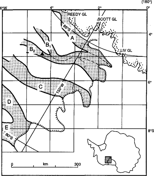
The ice streams that drain the West Antarctic ice sheet along the Siple Coast (Fig. 1) have been the focus of numerous glaciologic and geophysical investigations in recent years (Reference Alley and WhillansAlley and Whillans, 1991). A principal purpose for these studies has been to learn more about ice stream dynamics. In this paper, we investigate buried crevasses and associated strain features in the upper 85 m of a 250 km2 area of Ice Stream B. The data were collected during the 1991–92 field season using a high-resolution low-power impulse-type digitally recording ground-penetrating radar system.
Map of the ice streams (shaded) draining the West Antarctic ice sheet into the Ross Ice Shelf The solid triangle on Ice Stream B2 denotes the location of the experiments. The coordinate grid is derived by a simple transformation from polar geographic to rectangular coordinates (From Reference Shabtaie and BentleyShabtaie and Bently, 1987.)

The analysis consists of two parts. First, by tracking a target, we determine the variation in radar wave speed versus depth in the upper 85 m of the ice stream. Secondly, the shapes of diffraction hyperbolae recorded from buried linear features (crevasses, sharp folds or faults) are used to determine the depths and orientations of the buried features. The technique yields orientations from a single crossing and therefore allows effective mapping using survey-line separations of 1 km or more.
Field methods and data analysis
Instrumentation
The radar system comprised a GSSI Model SIR8 transmitter-receiver coupled to a single 80 MHz broadband transmit receive antenna with a 30 m cable. Navigation was provided by a combination of a bicycle-wheel odometer, a motion detector (used for sensing passage past grid poles accurately positioned by investigators at The Ohio State University (Reference Hulbe and WhillansHulbe and Whillans, 1994)) and an event-marking button. The data were logged directly from the CSSI receiver and navigation systems using a digital data-logging system designed and built at the University of Wisconsin. The sampling rate was 969 ± 12 MHz (1.032 ± 0.013ns sample−1). The data logger was controlled by an IBM lap-top computer and the entire system was powered from a 12V automobile battery. The relatively light weight and portability of the system allowed it to be mounted on a single Nansen sled; the antenna was towed on another Nansen sled 30 m behind. The sled train was towed by a Skidoo Alpine snowmobile. Where surface crevasses posed a danger, a second Skidoo was added 20 m behind the antenna sled for safety purposes. The snowmobile sled-sled-snowmobile arrangement was roped together; personnel were tied together on a separate rope system.
Radar-wave speed in firn
Investigators from the California Institute of Technology (Caltech) drilled several holes into and through the ice at Upstream B Camp (Fig. 1) during the 1992–92 field season (e.g. Reference Engelhardt, Hymphrey, Kamb and FahnestockEngelhardt and others, 1990). We used the radar system to record echoes from the descending (or ascending) metallic drill tip; from the echo times, the electromagnetic wave speed in the firn was calculated.
Two types of tips were used by Caltech, one 4.2 m long and one 1.6m long. Each hung on the end of a radar transparent nylon-reinforced hose. Our antenna was placed about 7 m from the top of the borehole. The data-acquisition rate varied between one and four traces per second, while drilling progressed at about 100 m h−1. The stem was tracked 12 times going up or down three different holes all within 100 m of each other. The depth of the stem was determined by calibrated meter wheels. The radar record was marked every 1 or 2 m in depth by a brief electronic pulse.
Velocity (v) versus depth (z) was calculated every 1 or 2 m from pulse travel-lime differences over 3–5 m depth intervals. A correction was made for the phase reversal from the conducting drill tip. Ray paths were assumed to be straight, an assumption that causes an error in wave speed of less than 1% at all depths.
Water introduced into the firn by Caltech’s hot-water drilling technique apparently had little effect on the measured wave speeds. As drilling progressed, large increases in echo strength were observed at specific stratigraphic levels. These changes were interpreted to mean that water was pooling at these particular levels. As long as the water content and thickness of the layer(s) did not change appreciably over the 1–3 min it took to penetrate (or withdraw through) 3–5 m of firn, and as long as that 3–5 m of firn did not include one of these wet layers, the effect of the water was removed by the travel time differencing.
The speeds are shown in raw form (Fig. 2a) and after a 5 m running mean has been applied (Fig. 2b). Also shown are least-squares regression lines of the form v(z) = a + bz fitted to the unsmoothed 0–50 m section. For the raw data (Fig. 2a), a= 213 ± l0 m µs−1, b = -0.87 ± 0.06 µs−1 and the square of the correlation coefficient is 0.63. For the smoothed data (Fig. 2b:, the correlation coefficient is 0.96; a and b are almost unchanged. Below 50 m, the wave speed is constant at 170 ± 4 µs−1.
Plots of wave speed versus depth at UpB. In each, the vertical line is at 170 m µs−1, the speed below 50 m. The sloping line is a least-squares regression-line fit to the data, and the curved line shows the wave speed expected from the known variation of density with depth. (a.) Individual measurements. (b.) .5 m running means.
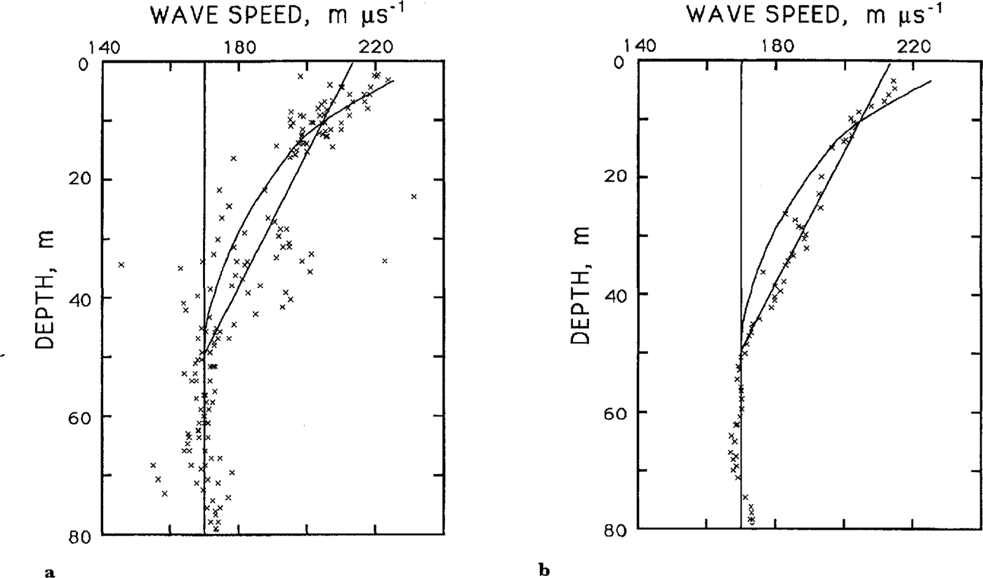
The apparent linear variation with depth is unexpected. The density-depth (ρ(z)) data presented by Reference Alley and BentleyAlley and Bentley (1988) show the expected decrease in dρ/ dz with depth downward to 50 m, where a solid-ice density of 0.90 Mg m−3 is reached; since v varies linearly with ρ (Bogorodsky and others, 1985), v(z) should show a similar form. We have plotted the expected v(z), calculated from ρ(z) using the linear relation of Reference Robin, Evans and BaileyRobin and others (1969), in Figure 2. Between 0 and 20 m, the measured and calculated wave speeds agree reasonably well, but between 25 and 50 m our measured velocities are consistently higher. (A further indication that water had little effect on the measurements.) Closely space gridded traverse lines in the vicinity of the drillholes showed buried crevasses very near two of the three drill locations. In both cases, the crevasse tops were located at about 25 m depth. We believe that propagation through crevasses is the likely cause of the unusually large wave speeds between 2.5 and 50 m. We note, however, that the data presented here cannot really differentiate between the two curves: the linear v(z) and the expected v(z) fall within 100 and 90%, respectively, of the standard deviations of the 5 m running means (not shown), For simplicity, we have used the linear relation for determining diffractor depths. The errors associated with the difference between the two curves are everywhere less than 1 m in depth and 10 years in age.
Shapes of theoretical diffraction hyperbolae
Many macroscopic strain features found on glaciers and ice sheets are linear in form. It is well known that, if the features are sharp enough, they appear as diffraction hyperbolae on radar records. Discontinuities associated with crevasses and faults obviously can cause diffraction hyperbolae: so can folding, if it is sharp compared to the curvature of the incident wave front.
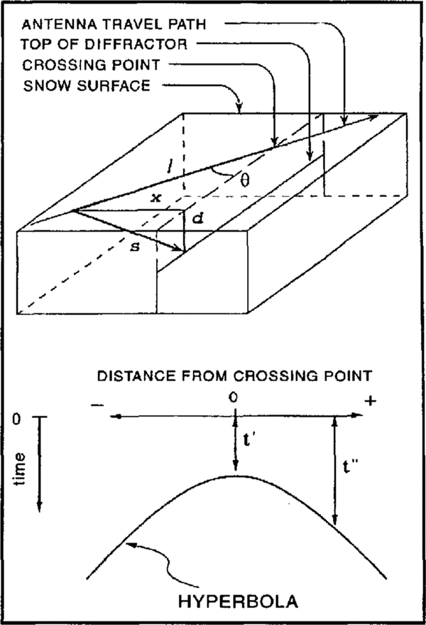
We derive a relation between hyperbola shape and crossing angle, assuming the diffractor is a straight line at a constant depth. From the geometry (Fig. 3), s
2 = x
2 + d
2, where s, x and d are slant, horizontal and vertical distances, respectively, from the antenna to the diffractor (Reference Jezek, Bentley and CloughJezek and others, 1979). Also,  and
 where t″ is the one-way travel time along s, v̄ is the average wave speed to depth d, ℓ is the distance along the traverse line from the antenna to the crossing point, θ is the crossing angle and t′ is the one-way travel time along d. For v = a + bz, we find by integration v̄ as a function of
 Then
Sketches showing the assumed geometry, the parameters used in the determination of crevasse orientation and how they relate to an observed hyperbola.


From Equation (1), sin2 θ can be calculated from the shape of the hyperbola; the sign of θ is not determined. Also, the ray path, s, is assumed to be straight. This introduces an error of less than 1% for incident angles of less than 45°, which constitute the majority of incident angles for any given hyperbola.
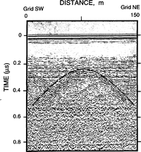
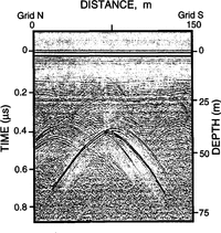
Several hyperbolae calculated from Equation (1) for different values of θ are shown in Figure 4. Calculated and measured hyperbolae from several crevasses that had known orientations (e.g. Fig. 5) agree within 5° or 10°, which is good considering that crevasses are not perfectly linear features.
Theoretical hyperbolae for linear diffractors at depths of 10 m (upper set) and 48 m (lower set) crossed at angles of 15° 30°, 60° and 90°.

A calculated hyperbola (dashed line) superimposed on an observed hyperbola. The crossing angle is 45°.
Description of buried features
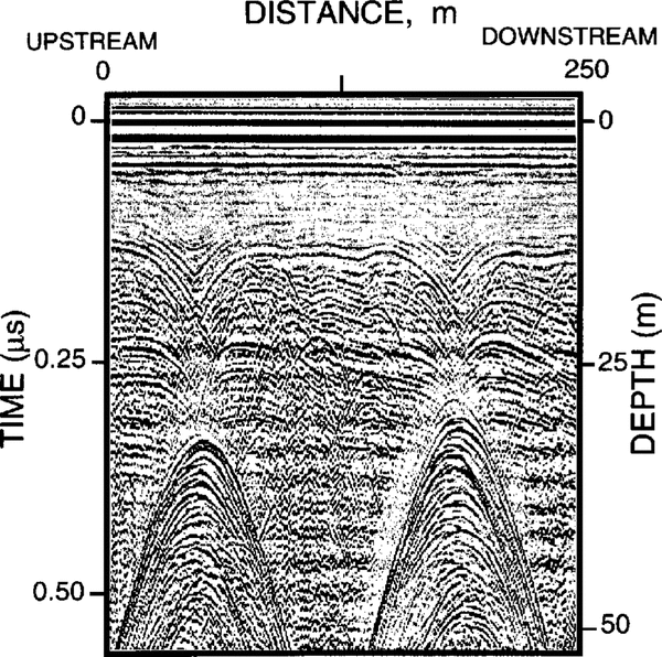
A number of different types of features produce hyperbolae and it is important to understand these differences if the hyperbolae are to be interpreted accurately. One type of near-surface crevasse produced what can be best described as single-sided hyperbolae (Fig. 6). While the surface expression of these crevasses was essentially linear, their edges were very irregular, and attempts to lower weights into them for measurement of depth were invariably thwarted by multiple snow bridges. Each side of these crevasses is characterized on the radargram by a separate set of single-armed hyperbolae with apices stacked from the surface to a depth of many meters. We interpret this as diffractions from a rough-walled crevasse, perhaps caused by simultaneous growth and burial.
Radargram we interpret as showing active crevasses with multiple snow bridges. Stacks of one-sided hyperbolae are particularly well shown in the features around 30 m from each end of the profile.

Another type of signature was observed from freshly opened, straight-edged, smooth-walled crevasses with burial depths of less than 1 m (Fig. 7). These show a single strong diffraction hyperbola at depth but almost no surface or wall signature. We associate the strong diffractions with the bottoms of the crevasses because in several cases the diffractor depths agreed with the measured depth of the corresponding crevasses. We attribute the lack of a signature from the top edges of these crevasses to their proximity to the surface and the antenna-beam angle, and the weak returns from the walls to a combination of the beam angle, the absence of snow bridges and the smoothness of the crevasse Walls.
Radargram from a very smooth-walled freshly opened crevasse. Hyperbolae near the surface can be seen only very faintly. This crevasse is about 0.7 m wide at the surface, about 37 m deep and covered by a 0.3 m thick Snow bridge.
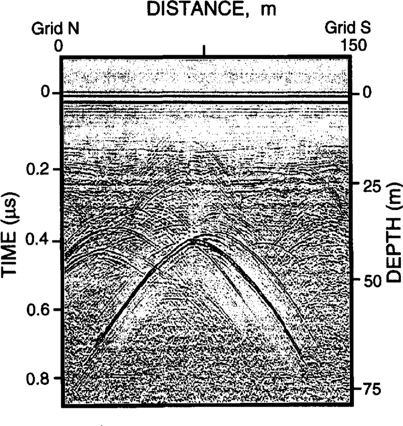
A third type of return was characterized by relatively weak hyperbolae originating from discontinuities associated with apparent faults (Fig. 8). The layering of the firn associated with these hyperbolae shows onsets of about 1 m, and these hyperbolae are only observed in areas of broad, gentle folding where there are few or no crevasses.
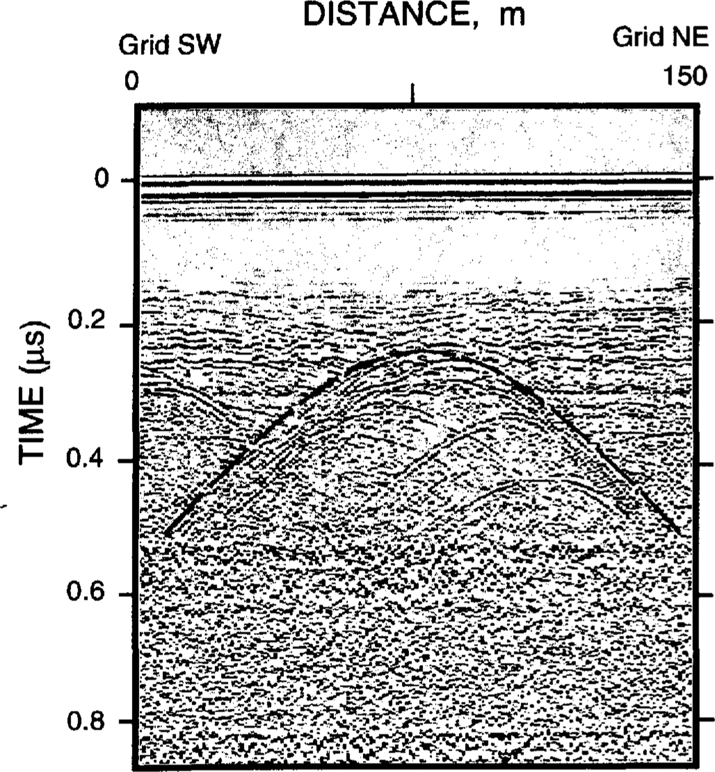
The fourth and most common type of hyperbola, however, we interpret as originating from buried snow bridges, because they are associated with distinct sags or synclines in the strata often bounded on each side by horizontal layers for 100m or more (Fig. 9). These hyperbolae occur in stacks that begin at the depth where the curvature of the syncline first exceeds the curvature of the wave front. Note that these hyperbolae provide a minimum depth to the original crevasse, since the first hyperbola in a stack is not necessarily correlated with the top of the crevasse.
Radargram showing weak hyperbolae originating from possible faults. The figure on the right is an interpreted section were hyperbolae associated with faults are dashed Lines. Offsets are about 1 m. The hyperbolae centered around 60 m across and 0.35µs depth probably have all off-nadir origin. The vertical disturbance that originates at 60 m along the surface is caused by a metallic grid pole.

Radargram showing hyperbolae associated with sagging bridges over buried crevasses. Note how the returns from sagging beds change downward into intersecting hyperbolae.

Orientation and distribution of buried features
Regardless of the nature of the sources for the hyperbolae, crossing angles can be determined on the assumption of linearity. The shapes of the hyperbolae are more sensitive to change in the crossing angle at shallow angles than at near-normal angles (Fig. 4). Shallow angles thus provide the most accurate orientations, and are encountered primarily on transverse transects (those oriented perpendicular to the flow). Longitudinal transects (oriented parallel to flow) generally provided larger numbers of crossings and thus provide a better estimate of crevasse density. Transverse and longitudinal transects were interpreted separately; the results agree to 10° or better. The ambiguity in the sign of the crossing angles was removed by using correlations between closely spaced or crossing grid lines where they existed, and then by assuming that the orientations vary smoothly between those locations.
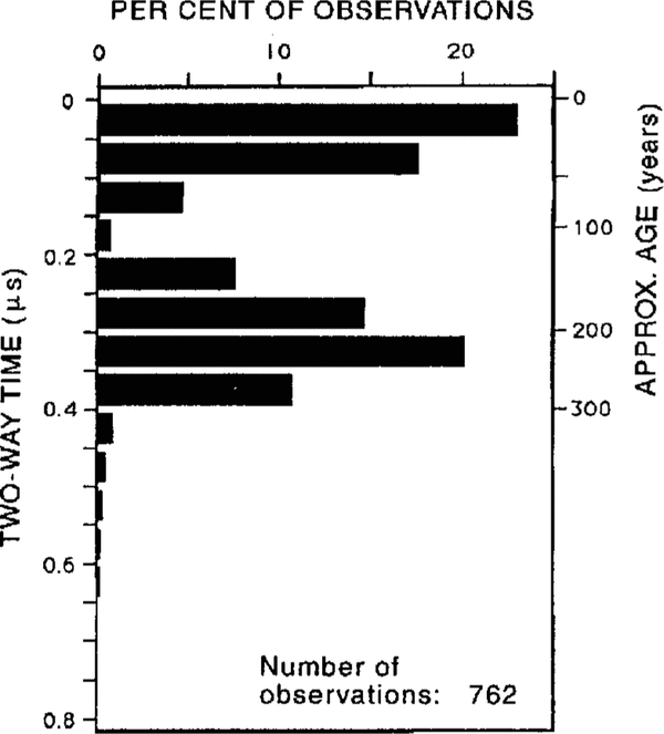
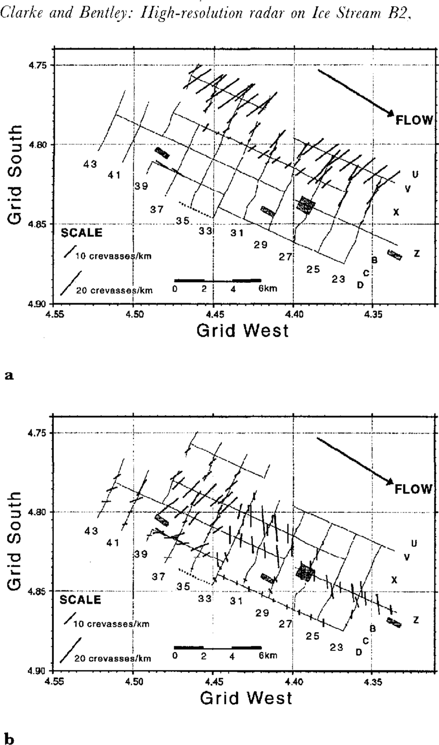
It is clear from a histogram of the distribution of hyperbolae with depth (Fig. 10) that there are two distinct crevasse populations. The shallow, young crevasses are currently active and are found in the grid northeastern part of the survey area (Fig. 11a). The orientations of the crevasses along the upstream northern edge of the grid are in good agreement with those mapped previously by Reference Whillans and van der VeenWhillans and others (1993). The crevasses downstream of that area tended to be buried slightly (hence the tail on the upper population), and therefore were not mapped by the photogrammetric technique employed by Whillans and others. The other crevasses, centered at a depth of about 30 m, have orientations that appear to vary rapidly or abruptly in the central part of the survey area (Fig. 11b). In reality, the two sets of crevasses probably intersect in this area. Figure 11b shows crevasses on either side of this area crossing the traverselines at approximately equal but opposite angles; since our method of determining orientation cannot distinguish positive from negative angles from a single traverse line, the two sets could easily be mixed.
Histogram of the number of diffractors versus depth. Only the shallowest hyperbola of a stack was counted.

Discussion and conclusions
The approximate age of burial for the deeper crevasse population can be calculated using present-day accumulation rates, and assuming that the crevasses reached the surface when they formed (Reference Whillans and van der VeenWhillans and others, 1993). (This is a reasonable assumption given that the sags associated with them are 20–30m wide (Fig. 9).) The accumulation rate in the survey area is 86 mm ice a−1 (Reference Alley and BentleyAlley and Bentley, 1988). It increases slowly upstream, averaging about 100 mm a−1over the first 200 km (Reference Whillans and BindschadlerWhillans and Bindschadler, 1988). Taking 100 ± 10mm a−1 as the accumulation rate (and post-depositional stretching as negligible) leads to an age at the depth of the peak in the deeper crevasse population of 210 ± 25 years (Fig. 10). Assuming a linear increase in ice speed from 100 m a−1 where crevasses are first observed to form, about 100km upstream, to 440ma −1 at the location of the grid (Reference Whillans and van der VeenWhillans and Van der Veen, 1993), we calculate the site of initial burial to be about 63 km upstream. This is in the lower reaches of the rather complex onset region. The likely interpretation is that the crevasses formed as the ice passed through this region. It also indicates that the ice stream has been exhibiting streaming behavior for at least the past 210 years, which is of interest given the apparent ephemeral nature of these ice streams (e.g. the recent stagnation of Ice Stream C about 130 years ago (Reference Retzlaff and BentleyRetzlaff and Bentley, 1993)).
We cannot reconstruct the state of stress that produced the buried crevasses because their subsequent strain history is not known. It is interesting, however, that a splayed crevasse pattern, as observed in the area grid west of line 35 (Fig. 11b), is the type expected in an area of transverse tension plus left-lateral shear, without longitudinal extension (Reference NyeNye, 1952; Reference Vornberger and WhillansVornberger and Whillans, 1990). If this pattern is relatively unaltered from its pre-burial configuration (a lair assumption given the near-center stream location of the crevasses, and the measurements of modern strain rate by Reference Whillans and van der VeenWhillans and others (1993)), it implies that longitudinal tension was not a factor in incorporating this particular ice into the ice stream.
We have no explanation for the crevasses to the grid east of line 35 nor for the 30° to 60° change in orientation over a distance of about 2 km. :Measured strain rates in the area are small (Reference WhillansWhillans, in press; Reference Whillans and van der VeenWhillans and others, 1993; Reference Hulbe and WhillansHulbe and Whillans, 1994) and show that rotation cannot account for the observed change over the time it takes the crevasses to travel 2 km, so the two sets of crevasses (grid east and west of line 35) either have markedly different post-burial strain histories, or more likely, formed in different stress regimes, even though their burial ages are approximately equal.
In one area along the grid southeastern edge of the survey, the radar returns showed virtually no visible stratigraphic disturbance (either crevassing or folding) down to 85 m, the maximum depth or our measurements (Fig. 11). Using the same assumptions as above for accumulation and velocity, the ice at 85 m is approximately 750 ± 80 years old, whereas travel time from the upper reaches of the ice stream to the location of the grid is only about 440 years. Apparently, this ice, and the ice adjacent to it to the grid south (toward the center of the stream), was incorporated into the ice stream without undergoing sufficient longitudinal strain (or side shear) to cause crevassing or folding, again implying that longitudinal tension was not a factor in incorporating this ice into the ice stream. Thus suggests that it might be a “raft” (Reference Whillam, Bolzan and ShabtaicWhillans and others, 1987, Reference Whillans, Jackson and Yseng1993), i.e. that it passed into the ice stream probably through the upstream onset zone (since it is near the center of the stream) as a single block.
Locations and orientations of the crevasses superimposed on a map of lines surveyed. Crevasse density and orientation are indicated by the length and orientation, respectively, of the heavy-line segments. Continuous lines are survey lines. Letters and numbers identify the lines of the strain grid. The survey-line segment with no crevasses or folds (D33–D36) is dashed. Gray-shaded boxes are areas where crevasse orientation was determined by correlation between closely spaced grid lines. (a.) The shallower set of crevasses (if Fig. 10). (b.) The deeper set (if Fig. 10). Deeper crevasses are present along the grid northeastern lines but they are obscured by the large number of younger crevasses in that area.
Acknowledgements
We wish to thank C. Liu and A.N. Novick for their assistance in the field and, in particular, N. Lord, without whom the project could not have been completed. We are grateful to I. M. Whillans and C. Hulbe at The Ohio State University for making the locations of the strain grid poles available to us. We also thank I. M. Whillans and two anonymous reviewers for helpful comments on the manuscript and R. W. Jacobel for discussions at VISAG. This work was supported by grant number DPP– 90–18530 from the U.S. National Science Foundation. This is contribution Number 541 of the University of Wisconsin-Madison, Geophysical and Polar Research Center.