1. Introduction
The compressible Navier–Stokes–Fourier (NSF) equations are routinely used to analyse gas flows when the Knudsen number (
 $Kn$
, the ratio between the mean free path and the macroscopic length of the system) is close to zero. For flows with large Knudsen numbers, the traditional low-order hydrodynamic equations are unable to predict many flow features, including the velocity slip and temperature jump at the walls, both being signatures of rarefaction effects. In molecular gases the flows are empirically classified based on Knudsen number (Kogan Reference Kogan1969; Bird Reference Bird1994): (i) continuum regime (
 $Kn\leqslant 10^{-2}$
), (ii) slip flow (
 $10^{-2}<Kn<0.1$
), (iii) transition flow (
 $0.1<Kn<10$
) and (iv) free-molecular flow (
 $Kn\geqslant O(10)$
). The slip and transition regimes fall under the category of ‘rarefied’ flows. The Boltzmann equation with appropriate boundary conditions can describe all flow regimes; unfortunately, however, it is not possible to solve the Boltzmann equation, even semi-analytically, for all
 $Kn$
. The NSF equations augmented by slip boundary conditions can describe the slip-flow regime reasonably well, but they fail when the Knudsen number is larger. One approach to model rarefied flows is to solve the Boltzmann equation via the direct simulation Monte Carlo (DSMC) method which is, however, computationally expensive (Bird Reference Bird1994); an alternative to DSMC is to use coarse-grained equations for extended sets of hydrodynamic fields. Such higher-order hydrodynamic equations, like the Burnett or super-Burnett equations (Burnett Reference Burnett1935) or Grad’s moment equations (Grad Reference Grad1949) or the regularized moment equations (Torrilhon & Struchtrup Reference Torrilhon and Struchtrup2004), seem to work well in the rarefied regimes of slip and transition flows up to a Knudsen number of
 $O(1)$
.
Rarefaction effects lead to non-Newtonian and non-Fourier transport coefficients, like the normal stress differences and ‘anisotropic’ thermal conductivity tensor, respectively, in molecular gases (Burnett Reference Burnett1935; Grad Reference Grad1949; Kogan Reference Kogan1969) as well as in dilute granular gases (Saha & Alam Reference Saha and Alam2014). At the level of hydrodynamic fields, one prototypical signature of rarefaction is the well-known ‘Knudsen-minimum’ effect (Knudsen Reference Knudsen1909) in Poiseuille flow: the mass-flow rate of a molecular gas decreases with increasing Knudsen number (
 $Kn$
), reaches a minimum at
 $Kn\sim O(1)$
and increases again with further increase in
 $Kn$
; this is also referred to as the ‘Knudsen-paradox’. The Knudsen-minimum/Knudsen-paradox has been predicted by analysing the steady Boltzmann equation with a BGK (Bhatnagar–Gross–Krook) collision term (Cercignani & Daneri Reference Cercignani and Daneri1963): the flow rate is inversely proportional to
 $Kn$
for small
 $Kn$
, but increases logarithmically (
 ${\sim}\text{log}Kn$
) for large
 $Kn$
. Another rarefaction-induced phenomenon in Poiseuille flow is the ‘bimodality’ of the temperature profile, i.e. the temperature is minimum at the channel centreline, with its maxima being located a few mean-free paths away from the centre; this was originally predicted by Tij & Santos (Reference Tij and Santos1994) and was confirmed later via DSMC simulations (Mansour, Baras & Garcia Reference Mansour, Baras and Garcia1997). The origin of the temperature bimodality has been attributed to the second-order correction terms in
 $Kn$
and hence this phenomenon belongs to the non-NSF regime (Aoki, Takata & Nakanishi Reference Aoki, Takata and Nakanishi2002).
Most granular flows of practical interest have Knudsen numbers larger than 0.01 (Goldhirsch Reference Goldhirsch2003; Galvin, Hrenya & Wildman Reference Galvin, Hrenya and Wildman2007; Forterre & Pouliquen Reference Forterre and Pouliquen2008; Gayen & Alam Reference Gayen and Alam2008; Khain, Meerson & Sasorov Reference Khain, Meerson and Sasorov2008; Rao & Nott Reference Rao and Nott2008; Rongali & Alam Reference Rongali and Alam2014; Saha & Alam Reference Saha and Alam2014) and therefore it is of interest to know whether the well-known signatures of rarefaction effects in molecular gases hold in granular gases. The latter are characterized by inelastic dissipation which is known to lead to some unexpected behaviour (Pöschel & Luding Reference Pöschel and Luding2001; Vega Reyes et al. Reference Vega Reyes, Santos and Garzo2010). Understanding the role of dissipation in rarefaction phenomena would help to formulate/test hydrodynamic-like theories and related boundary conditions for rarefied granular flows. Driven by this motivation, we focus on a simple flow configuration: the gravity-driven Poiseuille flow of a granular gas, for which no study exists on the Knudsen-minimum effect, but the temperature bimodality has been studied theoretically (Tij & Santos Reference Tij and Santos2004). We shall show, via simulation, that (i) the effect of dissipation on the above two rarefied phenomena is non-trivial, (ii) the wall roughness has a crucial role in the Knudsen-minimum effect and (iii) the characteristic features of temperature bimodality are at variance with the theoretical analysis of Tij & Santos (Reference Tij and Santos2004).
The simulation method for the gravity-driven flow of smooth inelastic hard disks in a channel is described in § 2, focusing on ‘dilute’ flows (the mean area fraction of particles being less than or equal to 0.01) for a range of Knudsen number (
 $O(0.001)\leqslant Kn\leqslant O(1)$
). The results on the mass-flow rate and the temperature profile are discussed in §§ 3.1 and 3.2, respectively, as functions of the normal restitution coefficient (
 $e_{n}$
), the wall roughness (
 ${\it\beta}_{w}$
) and the Knudsen number (
 $Kn$
). The conclusions are given in § 4.1. The present results shed some light on the range of validity of the granular hydrodynamic equations as discussed briefly in § 4.2. An appendix has been added that describes (i) the statistical steady state of our simulation (§ A.1), (ii) the hydrodynamic fields of granular Poiseuille flow (§ A.2), (iii) the possible role of normal stress difference in the flow rate (§ A.3) and (iv) the relative importance of dissipation and rarefaction on density profiles (§ A.4).
2. Simulation model for granular Poiseuille flow
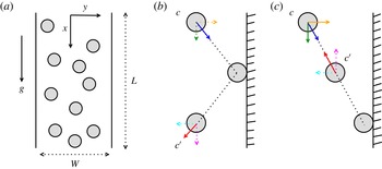
The flow configuration consists of a collection of circular disks flowing through a two-dimensional channel of width
 $W$
and length
 $L$
under the action of gravitational acceleration
 $g$
which is acting along the positive
 $x$
-direction, see figure 1(a). The channel is bounded by two rigid parallel walls at
 $y=\pm W/2$
, and the flow is assumed to be periodic along the
 $x$
-direction; the latter condition implies that a particle leaving the periodic boundary at
 $x=L$
re-enters through the opposite end at
 $x=0$
and vice versa (Mansour et al.
Reference Mansour, Baras and Garcia1997; Alam & Chikkadi Reference Alam and Chikkadi2010). As in the case of rapid granular flows (Goldhirsch Reference Goldhirsch2003), the particles move around randomly and are modelled as inelastic smooth hard disks (of diameter
 $d$
and mass
 $m$
) which interact via instantaneous binary collisions.
For smooth particles, the tangential velocity during a collision remains unchanged but the energy loss is manifested as a change in the normal component of the relative velocity via the following collision rule:
 $$\begin{eqnarray}\boldsymbol{c}_{12}^{\prime }\boldsymbol{\cdot }\boldsymbol{k}=-e_{n}(\boldsymbol{c}_{12}\boldsymbol{\cdot }\boldsymbol{k}),\end{eqnarray}$$
where
 $\boldsymbol{k}$
is the contact vector,
 $\boldsymbol{c}_{1}$
and
 $\boldsymbol{c}_{2}$
are the instantaneous velocities of disks 1 and 2, respectively, and
 $\boldsymbol{c}_{12}=\boldsymbol{c}_{2}-\boldsymbol{c}_{1}$
is the relative velocity. The restitution coefficient
 $e_{n}$
, the ratio between the post- and pre-collisional relative velocity between the colliding pair, is assumed to be a constant throughout the simulation.
Schematics of (a) granular Poiseuille flow and (b,c) the rules for wall–particle collisions: (b) reflected/specular and (c) bounce-back collisions.

2.1. Particle-level boundary condition
In addition to particle–particle collisions, the particles collide with the two rigid walls, see figure 1(b,c), and hence their post-collisional velocities are likely to be affected depending on the bulk ‘roughness’ of the walls. Assuming that the walls are rigid and massive (compared to the mass of a particle), the model for particle–wall collisions is taken as (Liss et al. Reference Liss, Conway and Glasser2002; Alam & Chikkadi Reference Alam and Chikkadi2010)
 $$\begin{eqnarray}c_{x}^{\prime }=-{\it\beta}_{w}c_{x}\quad \text{and}\quad c_{y}^{\prime }=-e_{w}c_{y},\end{eqnarray}$$
where
 $c_{i}$
is the velocity component of the colliding particle along the
 $i=x,y$
direction. For all simulations reported in this paper, we set
 $e_{w}=1$
in (2.2), i.e. the magnitude of the normal component of the velocity of a disk remains unchanged upon collision with a wall. The blue and red arrows emanating from the centres of the colliding particles in figure 1(b,c) represent typical pre- and post-collisional velocities, respectively, for two limiting cases of particle–wall collisions as described below.
The change in the tangential velocity component (
 $c_{x}$
) in (2.2) is parameterized by the ‘wall-tangential’ restitution coefficient
 ${\it\beta}_{w}$
, which characterizes the bulk roughness of the wall (Rao & Nott Reference Rao and Nott2008). The walls which reflect all particles (
 ${\it\beta}_{w}=-1$
) forward as in figure 1(b) do not cause any loss in the tangential momentum of incident particles and are called ‘smooth’ walls. On the other hand, the walls which bounce back (
 ${\it\beta}_{w}=1$
) particles in the direction of their incidence as in figure 1(c) reverse the tangential momentum of incident particles, and are called ‘perfectly rough’ walls. While the perfectly rough walls (
 ${\it\beta}_{w}=1$
) represent the ‘zero-slip’ condition at walls, the perfectly smooth walls (
 ${\it\beta}_{w}=-1$
) represent the ‘free-slip’ condition at walls (Chikkadi & Alam Reference Chikkadi and Alam2009). The intermediate case of
 ${\it\beta}_{w}=0$
, a linear combination of reflected (
 ${\it\beta}_{w}=-1$
) and bounce-back (
 ${\it\beta}_{w}=1$
) conditions, corresponds to the maximum energy loss for particle–wall collisions (which is proportional to
 ${\sim}(1-{\it\beta}_{w}^{2})$
for
 $e_{w}=1$
). Other values of
 ${\it\beta}_{w}\neq \pm 1$
represent a ‘mixed’ boundary condition which may be thought of as an analogue of Maxwell’s accommodation model (a fraction of wall–particle collisions is of specular-type and the rest are of bounce-back type) which is routinely used to model gas–surface interactions in kinetic theory (Cercignani Reference Cercignani2000).
In summary, the walls are modelled as rough-frictional surfaces with the particle–wall collision rule being given by a two-parameter model (2.2). The limits of free-slip and zero-slip conditions are achieved in this model by varying the wall tangential-restitution coefficient (i.e. the ‘bulk’ roughness of the walls) from
 ${\it\beta}_{w}\rightarrow -1$
to
 ${\it\beta}_{w}\rightarrow 1$
, respectively, see figure 15(a,b) in § A.2.
2.2. Simulation method and averaging
A previously developed (Alam & Chikkadi Reference Alam and Chikkadi2010) event-driven molecular dynamics code based on Lubachevsky’s (Reference Lubachevsky1991) algorithm is used to simulate the granular Poiseuille flow in the dilute regime. In order to prevent the inelastic collapse which is likely to occur at small values of the restitution coefficient, we implemented the TC-rule (Luding & McNamara Reference Luding and McNamara1998): if the collision time between particles is less than a critical time (
 $t_{c}\leqslant 10^{-9}$
) then
 $e_{n}$
is set to 1. The simulations are run for about 50 000 collisions per particle and the data are collected after the system has reached a statistical steady state which is ascertained by monitoring the constancy of the average kinetic energy,
 $E(t)=\sum _{i=1}^{N}(c_{xi}^{2}+c_{yi}^{2})/2N$
, per particle, see figure 13 in appendix A.
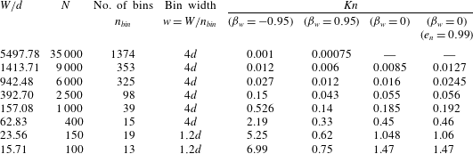
Since we are investigating rarefaction effects, the Knudsen number (the ratio between the mean-free path and a characteristic length scale of the system) must be calculated. In Poiseuille-type flows, the mean free path (
 ${\it\lambda}$
) varies across the channel width (see figure 14 in § A.1), and hence an average Knudsen number is defined via
 $$\begin{eqnarray}Kn\equiv \langle Kn(y)\rangle _{y}=\frac{\langle {\it\lambda}(y)\rangle _{y}}{W},\end{eqnarray}$$
where
 $\langle \cdot \rangle _{y}$
represents a spatial averaging over the channel width. To analyse rarefaction effects, a large range of (2.3) needs to be probed, which can be achieved in two ways: (i) vary the channel width
 $W/d$
and the number of particles
 $N$
for specified values of the channel length
 $L/d$
and the mean density,
 $$\begin{eqnarray}{\it\nu}_{av}=\frac{{\rm\pi}N}{4(L/d)(W/d)},\end{eqnarray}$$
or, (ii) for specified
 $W/d$
and
 $N$
, increase the channel length
 $L/d$
such that
 ${\it\nu}_{av}$
is decreased, which increases the mean-free path
 ${\it\lambda}$
(and hence
 $Kn$
increases) since
 ${\it\lambda}$
is inversely proportional to density. In both cases, the mean density is kept small (
 ${\it\nu}_{av}\leqslant 0.01$
) since we are focusing on a dilute granular gas. For all simulations reported here, we employed the first protocol to probe a range of
 $Kn\sim O(0.001)$
–
 $O(1)$
, see table 1 in § A.1; the same procedure was followed by Mansour et al. (Reference Mansour, Baras and Garcia1997) in the case of a molecular gas. The second protocol is computationally expensive, especially at large
 $Kn$
, since the channel width must be kept at
 $W/d\sim O(10^{3})$
or larger, but it was verified from a few case studies that the results reported here are robust irrespective of the protocol employed to vary the Knudsen number.
To extract hydrodynamic fields from the simulations, we divide the channel into an array of vertical bins, each of width
 $w$
(
 $w>d$
, see table 1 in appendix A) and then carry out ‘bin-wise’ averaging by collecting data in each bin after reaching a statistical steady state. The volume fraction
 ${\it\nu}$
, stream-wise velocity
 $U$
and granular temperature
 $T$
in the
 $i$
th bin (located at
 $y=y_{i}$
) are calculated from
 $$\begin{eqnarray}\displaystyle & \displaystyle {\it\nu}(y)=\frac{{\rm\pi}d^{2}}{4wL}\left\langle \mathop{\sum }_{i=1}^{N}{\it\delta}(y-y_{i})\right\rangle , & \displaystyle\end{eqnarray}$$
 $$\begin{eqnarray}\displaystyle & U(y)=\frac{\left\langle \displaystyle \mathop{\sum }_{i=1}^{N}c_{xi}(t){\it\delta}(y-y_{i})\right\rangle }{\displaystyle \left\langle \mathop{\sum }_{i=1}^{N}{\it\delta}(y-y_{i})\right\rangle }, & \displaystyle\end{eqnarray}$$
 $$\begin{eqnarray}\displaystyle & \displaystyle T(y)=\frac{\left\langle \displaystyle \mathop{\sum }_{i=1}^{N}\boldsymbol{C}_{i}(t)\boldsymbol{\cdot }\boldsymbol{C}_{i}(t){\it\delta}(y-y_{i})\right\rangle }{2\left\langle \displaystyle \mathop{\sum }_{i=1}^{N}{\it\delta}(y-y_{i})\right\rangle }, & \displaystyle\end{eqnarray}$$
 $\boldsymbol{C}_{i}(t)=\boldsymbol{c}_{i}(t)-U(y)\hat{\boldsymbol{x}}$
is the peculiar velocity (Chapman & Cowling Reference Chapman and Cowling1970) of particles, with
 $\hat{\boldsymbol{x}}$
being the unit vector along the
 $x$
-direction, and
 $\langle \cdot \rangle$
represents the time-averaging over a large number of snapshots of the system. For non-dimensionalization, the reference length, time and velocity scales are taken to be
 $W$
,
 $(W/g)^{1/2}$
and
 $(gW)^{1/2}$
respectively; the granular temperature (2.7) is scaled by
 $gW$
.
Typical cross-stream variations of the streamwise velocity and density are discussed in appendix A, see figure 15(a–d), and the characteristics of the temperature profiles are probed in § 3.2. The effect of inelastic dissipation on the microscopic (i.e. velocity distribution functions and two-point density and velocity correlations) and macroscopic (hydrodynamic profiles, slip velocity, rheology and density waves) fields of gravity-driven granular Poiseuille flow have been investigated in our previous works (Vijayakumar & Alam Reference Vijayakumar and Alam2007; Alam et al.
Reference Alam, Chikkadi and Gupta2009; Chikkadi & Alam Reference Chikkadi and Alam2009; Alam & Chikkadi Reference Alam and Chikkadi2010) for a range of densities, to which the reader is referred for related details. It must be noted that in the above works the simulations were carried out in a channel of width
 $W/d<100$
, and the Knudsen number was of order one (
 $Kn\sim O(1)$
) in the dilute regime and hence the rarefaction effects were not studied. On other hand, the focus of the present paper is to understand the role of inelastic dissipation on two well-known rarefaction effects in the gravity-driven Poiseuille flow of a dilute gas: (i) the Knudsen-minimum phenomenon (§ 3.1) and (ii) the bimodal shape of the temperature profile (§ 3.2).
3. Results and discussion: rarefaction
 $(Kn\neq 0)$
versus dissipation
$(e_{n}\neq 1)$


3.1. Does the Knudsen minimum exist in granular Poiseuille flow?
The dimensionless mass-flow rate is calculated from:
 $$\begin{eqnarray}Q=\frac{1}{{\it\nu}_{av}W\sqrt{gW}}\int _{-1/2}^{1/2}{\it\nu}(y)U(y)\,\text{d}y,\end{eqnarray}$$
where
 $U(y)$
and
 ${\it\nu}(y)$
are the streamwise velocity and density respectively. Equation (3.1) represents the mass-flow rate per unit width of the channel, since the length scale used is the width of the channel (
 $W$
) and the velocity scale is
 $\sqrt{gW}$
. In the dilute limit (
 ${\it\nu}\rightarrow 0$
), the mass flow rate
 $Q$
is likely to depend on (i) the Knudsen number
 $Kn$
, (ii) the wall roughness
 ${\it\beta}_{w}$
and (iii) the restitution coefficient
 $e_{n}$
, which we discuss separately in the following subsections.
3.1.1. Effect of wall roughness in the elastic limit:
$Q(Kn,{\it\beta}_{w},e_{n}\approx 1)$

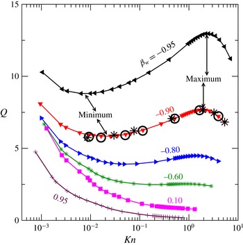
The variation of the flow rate
 $Q$
with Knudsen number
 $Kn$
is shown in figure 2 for a range of wall roughness [
 ${\it\beta}_{w}\in (-0.95,0.95)$
] in the elastic limit (
 $e_{n}=0.9999$
), with a mean density of
 ${\it\nu}_{av}=0.01$
; the results for the case of perfectly elastic collisions (
 $e_{n}=1$
) are almost identical with those of
 $e_{n}=0.9999$
, see the open circles in figure 2 for
 ${\it\beta}_{w}=-0.9$
. As discussed in § 2.2, the range of
 $Kn$
(2.3) in this figure has been achieved by varying the channel width
 $W/d$
and the number of particles
 $N$
which are listed in table 1 in § A.1. Focusing on the near-continuum limit (
 $Kn\rightarrow 0$
) of all curves in figure 2, we find that, irrespective of the value of the wall roughness
 ${\it\beta}_{w}$
, the flow rate decreases with increasing
 $Kn$
(for
 $Kn<0.01$
) which follows from Navier–Stokes hydrodynamics (Cercignani & Daneri Reference Cercignani and Daneri1963; Cercignani Reference Cercignani2000). On the other hand, for any specified value of
 $Kn$
, figure 2 also indicates that the mass-flow rate decreases with increasing wall roughness (
 ${\it\beta}_{w}>-1$
). This is because the smoother walls (
 ${\it\beta}_{w}\rightarrow -1$
) ensure a larger slip velocity (see below), leading to a higher flow rate compared to that in rough-walled channels (
 ${\it\beta}_{w}\rightarrow 1$
).
Effect of wall roughness (
 ${\it\beta}_{w}$
) on the variation of mass-flow rate (
 $Q$
) with average Knudsen number (
 $Kn$
) for a restitution coefficient of
 $e_{n}=0.9999$
. The mean density is
 ${\it\nu}_{av}=0.01$
and the channel length is
 $L/d=500$
; the open black circles represent the data for perfectly elastic collisions (
 $e_{n}=1$
) with a wall roughness of
 ${\it\beta}_{w}=-0.9$
and a channel length of
 $L/d=500$
, while the black star symbols represent the data for
 $e_{n}=1$
in a longer channel of length
 $L/d=1000$
. The range of
 $Kn$
is obtained by varying the channel width
 $W/d$
and the number of particles
 $N$
as listed in table 1 in § A.1.

Returning to the dependence of
 $Q$
on
 $Kn$
, we note from figure 2 that the flow rate decreases monotonically with increasing
 $Kn$
for channels with a wall-roughness of
 ${\it\beta}_{w}>-0.6$
. In contrast, for flows in relatively smooth-walled channels (see the top three curves in figure 2), the flow rate varies ‘non-monotonically’ with
 $Kn$
. More specifically, for the case of
 ${\it\beta}_{w}=-0.95$
(black curve), we find that the flow rate decreases with increasing
 $Kn$
, reaches a minimum at
 $Kn\approx 0.01$
, then increases, reaching a maximum at
 $Kn\approx 2.5$
, and finally decreases again with further increase in
 $Kn$
. The flow-rate curves for
 ${\it\beta}_{w}=-0.9$
and
 $-0.8$
are qualitatively similar to that for
 ${\it\beta}_{w}=-0.95$
, but the locations of
 $Q_{\mathit{min}}$
and
 $Q_{\mathit{max}}(Kn\neq 0)$
shift to larger and smaller values of
 $Kn$
respectively. For all data in figure 2 the channel length is set to
 $L/d=500$
, except for the black star symbols which represent additional data for
 $e_{n}=1$
with a larger channel length of
 $L/d=1000$
; this confirms that the overall shape of the
 $Q$
-curves does not depend on the length of the channel.
(a) Variation of
 ${\rm\Delta}Q=Q_{\mathit{max}}-Q_{\mathit{min}}$
, (3.2), with wall roughness
 ${\it\beta}_{w}$
for
 $e_{n}=0.9999$
. (b) Variations of the slip velocity (main panel) and the centreline velocity (inset) with
 $Kn$
for flows through a smooth-walled (
 ${\it\beta}_{w}=-0.95$
) channel. Other parameter values are as in figure 2.

The degree of non-monotonicity of the
 $Q$
-curves is quantified in terms of the difference between the local maximum and minimum of
 $Q$
(see figure 2),
 $$\begin{eqnarray}{\rm\Delta}Q=Q_{\mathit{max}}(Kn\neq 0)-Q_{\mathit{min}},\end{eqnarray}$$
whose variation with
 ${\it\beta}_{w}$
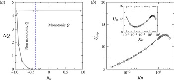
is shown in figure 3(a). This figure confirms that the flow-rate curves remain non-monotonic (i.e.
 ${\rm\Delta}Q>0$
) for flows in smooth-walled channels with a wall roughness of
 ${\it\beta}_{w}\leqslant -0.6$
. On the other hand, monotonic
 $Q$
-curves (i.e. decreasing
 $Q$
with increasing
 $Kn$
) prevail for flows through channels with roughness values of
 ${\it\beta}_{w}>-0.6$
.
To understand the origin of non-monotonic
 $Q$
-curves in figure 2, we probe the slip velocity
 $$\begin{eqnarray}U_{slip}\stackrel{def}{=}{\textstyle \frac{1}{2}}(U(\text{bin}=1)+U(\text{bin}=\text{last})),\end{eqnarray}$$
which is defined as the average of the streamwise velocities in two bins adjacent to stationary walls (see the velocity profiles in figure 15
a,b in appendix A). The variation of
 $U_{slip}$
(3.3) with
 $Kn$
is displayed in figure 3(b) for a wall roughness of
 ${\it\beta}_{w}=-0.95$
. It is seen that
 $U_{slip}$
increases with increasing
 $Kn$
, reaches a maximum at
 $Kn\sim 2$
and then starts decreasing with further increase in
 $Kn$
. This maximum slip velocity seems to be responsible for the local maximum in the flow rate at
 $Kn\sim 2$
for the case of
 ${\it\beta}_{w}=-0.95$
(see the topmost black curve in figure 2). Interestingly the centreline velocity
 $U_{0}$
, displayed in the inset of figure 3(b), follows the same non-monotonic trend with
 $Kn$
as that of the flow rate
 $Q$
. This is due to the fact that
 $U_{0}$
is a measure of the average velocity through the channel since the density variations across the channel (see figure 15
c,d in appendix A) at any
 $Kn$
remain small for
 $e_{n}\rightarrow 1$
.
(a) Effect of restitution coefficient
 $e_{n}$
on
 $Q$
for a wall roughness of
 ${\it\beta}_{w}=-0.9$
, with
 $e_{n}=1$
(red circles),
 $0.99$
(black squares) and
 $0.8$
(blue triangles). (b) Variation of
 ${\rm\Delta}Q$
, (3.2), with inelasticity
 $(1-e_{n})$
for
 ${\it\beta}_{w}=-0.9$
. (c) Phase diagram in the (
 ${\it\beta}_{w},1-e_{n}$
)-plane, delineating the regions of non-monotonic (
 ${\rm\Delta}Q>0$
) and monotonic (
 ${\rm\Delta}Q=0$
) mass-flow rates; the inset shows the definition of
 ${\rm\Delta}Q$
, (3.2), with representative data for
 $e_{n}=0.9999$
and
 ${\it\beta}_{w}=-0.95$
. Other parameter values are as in figure 2 and listed in table 1.

3.1.2. Effects of inelastic dissipation
$(e_{n}<1)$
and rarefaction
$(Kn>0)$
: the phase diagram


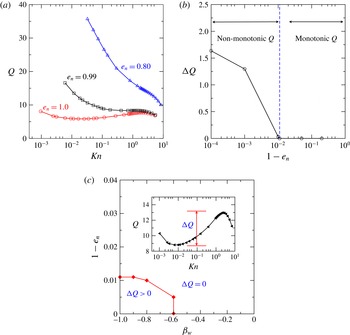
The effect of inelastic dissipation on the mass-flow rate
 $Q$
can be ascertained from figure 4(a) which compares three
 $Q$
-curves for
 $e_{n}=1.0$
(red circles), 0.99 (black squares) and 0.8 (blue triangles). For all cases, the wall roughness is set to
 ${\it\beta}_{w}=-0.9$
such that
 $Q(Kn)$
is non-monotonic in the elastic limit (
 $e_{n}=1.0$
) as indicated by the red-circle curve. In contrast, the black-square curve for
 $e_{n}=0.99$
indicates that
 $Q(Kn)$
decreases sharply up to
 $Kn\approx 0.2$
, and there is a plateau at around
 $Kn=O(1)$
, beyond which
 $Q(Kn)$
decreases again with increasing
 $Kn$
. Decreasing the restitution coefficient to
 $e_{n}=0.8$
(blue-triangle curve) makes
 $Q(Kn)$
a monotonically decreasing function of
 $Kn$
. The decrease of
 $Q(Kn)$
with increasing
 $Kn$
becomes sharper with further decrease of
 $e_{n}$
(not shown).
Figure 4(b) summarizes the effects of
 $e_{n}$
on the flow rate as a phase diagram in the (
 ${\rm\Delta}Q,1-e_{n}$
)-plane, with
 ${\rm\Delta}Q$
being defined in (3.2). It is seen that
 ${\rm\Delta}Q>0$
for
 $(1-e_{n})\leqslant 0.011$
and zero (i.e.
 $Q$
is monotonically decreasing with increasing
 $Kn$
) otherwise; these overall observations hold for other values of
 ${\it\beta}_{w}<-0.6$
. The information provided in figures 3(a) and 4(b) can be combined to obtain a phase diagram in the (
 ${\it\beta}_{w},1-e_{n}$
)-plane as depicted in figure 4(c). The regions on the left and right of the broken line (marked with diamonds) in figure 4(c) represent the regimes of ‘non-monotonic’ (
 ${\rm\Delta}Q>0$
) and ‘monotonic’ (
 ${\rm\Delta}Q=0$
) mass-flow rates respectively. We conclude from this phase diagram that the Knudsen-minimum effect is absent in granular Poiseuille flow (i) for
 $e_{n}<0.989$
, irrespective of the value of the wall roughness, and (ii) for relatively rougher walls with
 ${\it\beta}_{w}>-0.6$
at any
 $e_{n}$
.
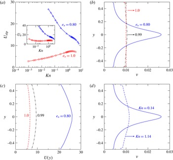
(a) Variations of slip velocity (main panel) and centreline velocity (inset) with
 $Kn$
for
 $e_{n}=0.8$
(blue triangles) and
 $e_{n}=1.0$
(red circles). (b,c) Effect of
 $e_{n}$
on (b) density and (c) velocity profiles at
 $Kn\approx 0.1$
; the blue solid, black dot-dashed and red dashed lines refer to
 $e_{n}=0.8$
, 0.99 and 1 respectively, in a channel of width
 $W/d=549.77$
with
 $N=3500$
particles. (d) Comparison of the density profiles for
 $Kn=0.14$
(solid line,
 $W/d=549.77$
and
 $N=3500$
) and
 $Kn=1.14$
(dashed line,
 $W/d=196.35$
and
 $N=1250$
) at
 $e_{n}=0.8$
. In all panels, the wall roughness is
 ${\it\beta}_{w}=-0.9$
with other parameter values as in figure 2.

3.1.3. Role of Knudsen number and the anomalous variation of slip velocity
To understand the dependence of
 $Q(Kn,e_{n})$
on
 $Kn$
for specified
 $e_{n}$
, we show the variations of the slip velocity
 $U_{slip}$
and the centreline velocity
 $U_{0}$
with
 $Kn$
, respectively, in the main panel and the inset of figure 5(a) for
 $e_{n}=0.8$
and 1.0. For this parameter combination,
 $U_{slip}$
increases with increasing
 $Kn$
for elastic (
 $e_{n}=1$
) particles; however, it follows a completely opposite trend when the restitution coefficient is reduced to
 $e_{n}=0.8$
. The latter finding is dubbed anomalous since
 $U_{slip}$
is known to increase with increasing
 $Kn$
in a molecular gas. In any case, the decrease of
 $U_{slip}$
with increasing
 $Kn$
is responsible for the continual decrease of
 $Q$
with increasing
 $Kn$
for moderately dissipative (
 $e_{n}=0.8$
) particles in smooth-walled channels.
Figure 5(a) further indicates that increasing dissipation results in larger values for both the slip velocity
 $U_{slip}$
(main panel) and the centreline velocity
 $U_{0}$
(inset), and hence the flow rate would increase with decreasing
 $e_{n}$
at any
 $Kn$
, as we found in figure 4(a). It is noteworthy that the latter effect becomes more prominent as
 $Kn$
decreases progressively towards zero, which can be explained as follows. The density profiles in figure 5(b) confirm a significant density variation across the channel width for
 $e_{n}=0.8$
(blue solid line) in comparison to nearly flat density profiles for
 $e_{n}=0.99$
(black dot-dashed line) and 1.0 (red-dashed line); the Knudsen number is set to
 $Kn\approx 0.1$
for three data sets. Overall, the particles tend to migrate towards the channel centreline where the shear rate is low with increasing dissipation (and vice versa), leading to the formation of particle-rich and particle-depleted regions near the centreline and the walls respectively. The relatively particle-depleted regions near the walls for
 $e_{n}=0.8$
imply a more rarefied regime, resulting in an increased slip velocity with decreasing
 $e_{n}$
for specified
 $Kn$
. This finding of ‘transverse clustering’ of particles (see figure 5
b) with decreasing
 $e_{n}$
, in conjunction with enhanced bulk velocities (figure 5
c), would result in enhanced flow rate (3.1) in the same limit. (A related effect with decreasing
 $e_{n}$
is the ‘finite/measurable’ normal stress differences that may also aid in enhancing the mass-flow rate, see figure 16 and the related discussion in § A.3.) It must be noted, however, that the above argument of clustering-enhanced flow rate is strictly valid in the continuum limit (
 $Kn\rightarrow 0$
) where the rarefaction effects can be neglected.
Returning to the effects of Knudsen number on the spatial distribution of particles, we compare the density profiles for
 $Kn=1.14$
(dashed line) and 0.14 (solid line) in figure 5(d). It is clear that, with other parameters being fixed, increasing
 $Kn$
leads to a more homogeneous distribution of particles across the channel width, dubbed ‘declustering’. The relatively homogeneous distribution of particles at larger
 $Kn$
results in more collisions with the walls (compared to the case for
 $Kn=0.14$
) and hence a larger energy loss near the walls, leading to a lower slip velocity with increasing
 $Kn$
at
 $e_{n}=0.8$
. Therefore, the competing effects of (i) the dissipation-induced clustering and (ii) the rarefaction-induced declustering along the wall-normal direction are responsible for the ‘anomalous’ decrease of
 $U_{slip}$
with increasing
 $Kn$
at lower values of
 $e_{n}$
(the blue curve in figure 5
a). For a related discussion on the dissipation-dominated and
 $Kn$
-dominated flow regimes, we refer to § A.4.
3.1.4. Summary and implications
Collectively, figures 2–4 confirm that the Knudsen-minimum effect is absent in a granular Poiseuille flow when the restitution coefficient is less than
 $0.99$
, irrespective of the roughness (
 ${\it\beta}_{w}$
) of channel walls. Only for quasi-elastic (
 $e_{n}\approx 1$
) particles flowing through a channel with very smooth walls (
 ${\it\beta}_{w}\sim -1$
), do we see evidence of a local minimum, which appears at a Knudsen number of
 $Kn\sim O(0.01)$
and, more interestingly, the flow rate can be maximum at finite
 $Kn\sim O(1)$
. The latter finding has important implications: the maximum flow rate at finite
 $Kn$
can be achieved by choosing an appropriate channel width (
 $W/d$
) with very smooth walls. At sufficiently small values of
 $e_{n}$
, the inelastic dissipation overcomes the competing effect of rarefaction, which is responsible for the observed monotonic variation of the mass-flow rate for
 $e_{n}<0.99$
.
Our findings on the Knudsen-minimum effect in granular Poiseuille flow seem to be at odds with reference to what is known in a molecular gas (Knudsen Reference Knudsen1909; Cercignani & Daneri Reference Cercignani and Daneri1963). One possible reason is that our boundary conditions (§ 2.1) are different from the ‘thermal-wall’ boundary conditions (that are used to model the Poiseuille flow of a molecular gas (Cercignani Reference Cercignani2000)) in some fundamental ways. This issue can be resolved if the present ‘athermal’ boundary conditions could be mapped into ‘effective’ thermal wall conditions by a priori specifying (i) a wall temperature and (ii) the momentum accommodation coefficients. While it is not clear how to specify the ‘granular’ temperature for a ‘stationary’ wall, the latter, (ii), requires some knowledge about the velocity distribution functions of incident and reflected particles near the walls. Previous works (Vijayakumar & Alam Reference Vijayakumar and Alam2007; Alam & Chikkadi Reference Alam and Chikkadi2010) suggest that such wall-distribution functions in granular Poiseuille flow can deviate significantly from a Maxwellian if the walls are rough, and therefore the simple rules to reflect/bounce back the particles (based on a Maxwellian distribution at some wall-temperature, Mansour et al.
Reference Mansour, Baras and Garcia1997; Aoki et al.
Reference Aoki, Takata and Nakanishi2002) are unlikely to hold for a granular gas. A systematic resolution of these issues may help to understand the absence of the Knudsen-minimum effect in granular/athermal Poiseuille flow with relatively rough walls (
 ${\it\beta}_{w}>-0.6$
) at any restitution coefficient.
3.2. Bimodality of granular temperature: rarefaction or dissipation driven?
Here we characterize the temperature profiles in a dilute granular Poiseuille flow, and attempt to make a connection with the well-known ‘bimodal’ shape (Tij & Santos Reference Tij and Santos1994), with a temperature minimum at the centre of the channel and two local maxima positioned symmetrically away from
 $y=0$
, in its molecular gas counterpart. The primary goal is to unveil the origin of the temperature bimodality in the granular Poiseuille flow. All results in this section are presented for
 ${\it\beta}_{w}=0$
, which corresponds to a mixed boundary condition with equal contributions from bounce-back (
 ${\it\beta}_{w}=1$
) and specular/reflected (
 ${\it\beta}_{w}=-1$
) particle–wall collisions, but we have verified that the following observations hold for any
 $-1<{\it\beta}_{w}<1$
.
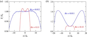
Figures 6(a) and 6(b) display the temperature profiles for the case of perfectly elastic (
 $e_{n}=1$
) and inelastic (
 $e_{n}=0.99$
) collisions respectively. The temperature has been normalized by its centreline value (
 $T_{0}=T(y=0)$
) which is plotted against
 $y/{\it\lambda}_{0}$
, where
 ${\it\lambda}_{0}$
is the centreline mean-free path. (The corresponding density profiles are shown in figure 17(a,b) in § A.4.) The two curves in each panel represent data for channels of different widths that can be mapped to different values of average Knudsen number (
 $Kn\sim 0.01$
and 0.1, from (2.3); see table 1 in § A.1). For the case of perfectly elastic collisions (
 $e_{n}=1$
) in figure 6(a), it is seen that the temperature profile has a maximum at
 $y=0$
for
 $Kn=0.012$
, but the one at
 $Kn=0.11$
has a local minimum at
 $y=0$
, with two maxima being located symmetrically away from
 $y=0$
. Overall the temperature profile for
 $e_{n}=1.0$
is unimodal at lower values of
 $Kn$
and becomes bimodal at larger
 $Kn$
. In contrast, for a granular gas (
 $e_{n}=0.99$
), the bimodal shape of the temperature profile persists even at lower values of
 $Kn\sim 0.01$
as confirmed in figure 6(b). More importantly, the degree of bimodality (
 ${\sim}(T_{\mathit{max}}-T_{0})$
, (3.4)) has increased markedly with decreasing
 $Kn$
for
 $e_{n}=0.99$
. This seemingly opposite behaviour for
 $e_{n}=1$
and
 $e_{n}=0.99$
can be resolved if we know the origin of the temperature bimodality in granular/athermal Poiseuille flow.
Temperature profiles at different
 $Kn$
for (a) perfectly elastic (
 $e_{n}=1$
) and (b) inelastic (
 $e_{n}=0.99$
) particles; the parameter values are set to
 ${\it\nu}_{av}=0.01$
,
 $L/d=500$
and
 ${\it\beta}_{w}=0$
in both panels. While in (a) the Knudsen numbers of
 $Kn=0.012$
and 0.11 are achieved with parameters of
 $(W/d,N)=(1178.09,7500)$
and
 $(W/d,N)=(235.61,1500)$
respectively, in (b)
 $Kn=0.011$
and 0.12 correspond to
 $(W/d,N)=(1570.79,10\,000)$
and
 $(W/d,N)=(235.61,1500)$
respectively.

3.2.1. Origin of temperature bimodality
The primary characteristic feature of the bimodal shape of the temperature profile, such as those in figure 6, is the ‘excess’ temperature ratio,
 ${\rm\Delta}T$
, which is defined as
 $$\begin{eqnarray}{\rm\Delta}T=\frac{(T_{\mathit{max}}-T_{0})}{T_{0}},\end{eqnarray}$$
where
 $T_{0}$
is the temperature at the channel centreline (
 $y=0$
) and
 $T_{\mathit{max}}$
is the maximum temperature. Clearly,
 ${\rm\Delta}T=0$
and
 ${>}0$
for unimodal and bimodal temperature profiles respectively. The larger the value of
 ${\rm\Delta}T$
, the larger is the deviation from a unimodal profile, and hence
 ${\rm\Delta}T$
is also a measure of the degree of temperature bimodality. To find out whether there is indeed a local minimum of the temperature profile at
 $y=0$
, we need to evaluate its second derivative
 $T^{\prime \prime }(y=0)$
: the temperature has a local maximum or minimum at
 $y=0$
depending on whether
 $$\begin{eqnarray}T^{\prime \prime }(0)\equiv \frac{\text{d}^{2}T}{\text{d}y^{2}}(y=0)\leqslant 0\quad \text{or}\quad T^{\prime \prime }(0)>0,\end{eqnarray}$$
respectively.
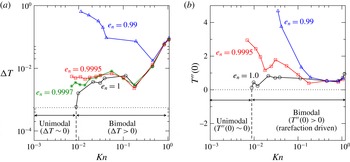
Figures 7(a) and 7(b) display the variations of
 ${\rm\Delta}T$
and
 $T^{\prime \prime }(y=0)$
, respectively, with Knudsen number
 $Kn$
. In each panel, the curves represent data for different restitution coefficients. The black-circle curves for
 $e_{n}=1$
in figure 7(a,b) confirm that the temperature profile for elastically colliding particles undergoes a transition from a unimodal (
 ${\rm\Delta}T\approx 0$
and
 $T^{\prime \prime }(y=0)\approx 0$
) to a bimodal (
 ${\rm\Delta}T>0$
and
 $T^{\prime \prime }(y=0)>0$
) shape at some small but finite value of
 $Kn=Kn_{c}\approx 0.01$
. Therefore, the origin of temperature bimodality in the Poiseuille flow of a molecular gas is tied to the rarefaction effect (Tij & Santos Reference Tij and Santos1994; Mansour et al.
Reference Mansour, Baras and Garcia1997) since it occurs at finite values of Knudsen number.
The red-square lines in figure 7(a,b) indicate that both
 ${\rm\Delta}T$
and
 $T^{\prime \prime }(0)$
are positive for all
 $Kn>0$
at
 $e_{n}=0.9995$
(since the
 ${\rm\Delta}T$
-curve develops a plateau and does not seem to decrease as
 $Kn\rightarrow 0$
and
 $T^{\prime \prime }(0)$
increases in the same limit), implying that the corresponding temperature profile is bimodal. Further decreasing the restitution coefficient (
 $e_{n}=0.99$
, see the blue lines with triangles in both panels) enhances the values of both
 ${\rm\Delta}T$
and
 $T^{\prime \prime }(0)$
markedly at lower values of
 $Kn<0.1$
. In contrast, we find that the effect of dissipation on both
 ${\rm\Delta}T$
and
 $T^{\prime \prime }(0)$
diminishes with increasing
 $Kn$
, and the respective curves for different
 $e_{n}$
coincide at
 $Kn\sim O(1)$
and beyond. Collectively, therefore, figure 7(a,b) confirms that the inelastic dissipation is the driving factor for the genesis of temperature bimodality in the continuum limit of
 $Kn\rightarrow 0$
, and the rarefaction effect prevails at large enough
 $Kn$
.
Variations of (a) excess temperature,
 ${\rm\Delta}T$
, and (b)
 $\text{d}^{2}T/\text{d}y^{2}(y=0)$
with average Knudsen number
 $Kn=\langle Kn(y)\rangle$
for different restitution coefficients of
 $e_{n}=1$
(black circles),
 $e_{n}=0.9995$
(red squares),
 $e_{n}=0.9997$
(green-stars) and 0.99 (blue triangles). The parameter values are set to
 ${\it\nu}_{av}=0.01$
and
 ${\it\beta}_{w}=0$
, with channel dimensions (for different
 $Kn$
) being listed in table 1.

3.2.2. The phase diagram: rarefaction versus dissipation
It is clear from figure 7(a) that the temperature profile remains bimodal (
 ${\rm\Delta}T>0$
) for
 $e_{n}\leqslant 0.9995$
at any
 $Kn$
. On the other hand, extrapolating the green line (for
 $e_{n}=0.9997$
), marked by the star symbols in figure 7(a), for small
 $Kn$
yields
 ${\rm\Delta}T=0$
at
 $Kn_{c}\approx 0.007$
, below which the temperature profile becomes unimodal. Therefore, the ‘unimodal-to-bimodal’ transition would occur for a very small range of restitution coefficient
 $e_{n}\in (0.9997,1)$
in the limit
 $Kn\rightarrow 0$
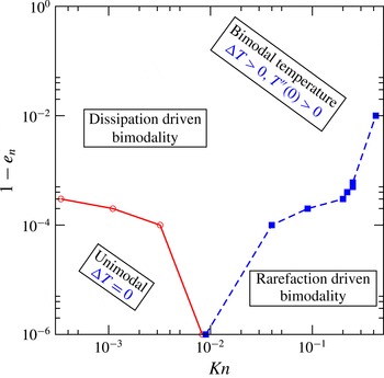
. The above findings are summarized in figure 8 as a phase diagram in the (
 $Kn,1-e_{n}$
)-plane. The red line with circles represents a phase boundary, to the left and right of which the temperature profile is unimodal and bimodal respectively. Note that the region of unimodal temperature in the (
 $Kn$
,
 $1-e_{n}$
)-plane is very small.
In the bimodal region of the phase diagram in figure 8, two distinct mechanisms compete with each other: (i) the temperature bimodality near the continuum limit (
 $Kn\sim 0$
) is driven solely by inelastic dissipation, but (ii) the rarefaction-driven bimodality remains active beyond a critical Knudsen number
 $Kn>Kn_{c}(e)>0$
as in a molecular gas. The latter mechanism would take over from the dissipation-driven mechanism at large enough
 $Kn$
(for a given
 $e_{n}$
) since the particle–wall collisions dominate over particle–particle collisions at large
 $Kn$
and therefore the collisional dissipation is likely to have a minor role in the ‘bulk’ dynamics of the flow at sufficiently large
 $Kn$
. These arguments suggest that there must be another phase boundary in the (
 $Kn,1-e_{n}$
)-plane that would demarcate (i) the dissipation-driven bimodality from (ii) the rarefaction-driven bimodality. This is marked by the blue-dashed line in figure 8, to the left and right of which the mechanisms (i) and (ii), respectively, are operative. The square symbols on this phase-boundary have been obtained from figure 7(b) as follows: each curve of
 $T^{\prime \prime }(0)$
is fitted via a polynomial in
 $Kn$
and then we determine the value of
 $Kn$
at which its slope,
 $\text{d}/\text{d}Kn(T^{\prime \prime }(0))$
, saturates approximately to zero (within 5 %).
Phase diagram in the (
 $Kn,1-e_{n}$
)-plane, delineating the regions of unimodal (
 ${\rm\Delta}T=0$
) and bimodal (
 ${\rm\Delta}T>0$
and
 $\text{d}^{2}T/\text{d}y^{2}(y=0)>0$
) temperature profiles (red solid line). The blue dashed line approximately splits the bimodal regime into two parts: (i) rarefaction-induced and (ii) dissipation-induced bimodality. The parameter values are as in figure 7.

Effect of restitution coefficient
 $e_{n}$
on granular temperature profiles (main panels); the insets show the variations of the excess temperature
 ${\rm\Delta}T$
(3.4), denoted by black circles) and the centreline temperature
 $T_{0}$
(denoted by red squares) with
 $e_{n}$
. Parameter values are (a)
 ${\it\nu}_{av}=0.01$
(
 $W/d=400$
and
 $L/d=294.5$
) and (b)
 ${\it\nu}_{av}=0.005$
(
 $W/d=400$
and
 $L/d=589$
), with
 $N=1500$
. (c) Same as in (b), but in a wider channel
 $W/d=800$
with
 $N=3000$
.

3.2.3. Excess temperature and its variation with
$e_{n}$

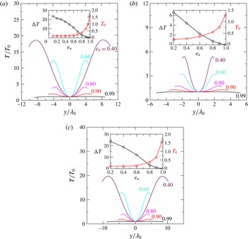
The temperature profiles at much lower values of
 $e_{n}$
are displayed in figure 9(a–c); these simulations have been carried out for
 ${\it\nu}_{av}=0.01$
(figure 9
a:
 $W/d=400$
,
 $L/d=294.5$
and
 $N=1500$
),
 ${\it\nu}_{av}=0.005$
(figure 9
b:
 $W/d=400$
,
 $L/d=589$
and
 $N=1500$
), and
 ${\it\nu}_{av}=0.005$
(figure 9
c:
 $W/d=800$
,
 $L/d=589$
and
 $N=3000$
). For all three case studies, the minimum temperature is found to occur at the channel centreline, and the maximum temperature away from
 $y=0$
. A comparison between figure 9(a) (
 ${\it\nu}_{av}=0.01$
) and figure 9(b) (
 ${\it\nu}_{av}=0.005$
) indicates that the maximum temperature and its location depend on the mean density; on the other hand, fixing the mean density to 0.005 but increasing the channel width from 400 (figure 9
b) to 800 (figure 9
c) also changes the value of
 $T_{\mathit{max}}$
and its location. Since the channel width is the same for both figures 9(a) and 9(b), decreasing the mean density from 0.01 to 0.005 implies a higher value for the Knudsen number (
 $Kn=\langle {\it\lambda}\rangle /W\sim {\it\nu}_{av}^{-1}$
); similarly, increasing the channel width 400 (figure 9
b) to 800 (figure 9
c) would result in decreased
 $Kn\propto W^{-1}$
. We shall show in § 3.2.4 that the results remain qualitatively similar for different parameter sets as long as the Knudsen numbers are of the same order.
Each inset of figure 9(a–c) indicates that the centreline temperature
 $T_{0}$
(marked by the red line) decreases with increasing dissipation (
 ${\sim}(1-e_{n}^{2})$
). The variation of the excess temperature ratio,
 ${\rm\Delta}T$
, (3.4), is also shown (marked by the black-circle line) as a function of
 $e_{n}$
in each inset. It is clear that
 ${\rm\Delta}T$
increases monotonically with decreasing
 $e_{n}$
which implies that the degree of temperature bimodality becomes more pronounced with increasing dissipation/inelasticity. This finding is in apparent contradiction with Tij & Santos (Reference Tij and Santos2004) who predicted that
 ${\rm\Delta}T$
decreases with decreasing
 $e_{n}$
from the elastic limit up to a value of
 $e_{n}\sim 0.4$
and increases subsequently for
 $e_{n}<0.4$
(see § 3.2.4).
3.2.4. Comparison of excess temperature with theory
Let us make a quantitative comparison of our simulation with the analysis of Tij & Santos (Reference Tij and Santos2004) who solved the inelastic Boltzmann equation (with a BGK-type collision model) subjected to a constant gravitational force and a stochastic (white noise) thermostat. The role of the stochastic thermostat was to heat the granular gas such that it compensates the loss of energy due to collisional cooling, yielding a ‘uniform’ state about which a Chapman–Enskog-type expansion was carried out by treating the body force as a small parameter (which is proportional to the centreline Knudsen number
 $Kn_{0}$
). Under these assumptions, they confirmed that while the Navier–Stokes equations (for a dilute granular gas) yield a temperature maximum,
 $$\begin{eqnarray}\left(\frac{\partial ^{2}T}{\partial y^{2}}\right)_{y=0}=0\quad \text{and}\quad \left(\frac{\partial ^{4}T}{\partial y^{4}}\right)_{y=0}<0,\end{eqnarray}$$
at the channel centreline (
 $y=0$
), the incorporation of
 $O(Kn^{2})$
-corrections results in
 $$\begin{eqnarray}\left(\frac{\partial ^{2}T}{\partial y^{2}}\right)_{y=0}>0,\end{eqnarray}$$
implying a local minimum at
 $y=0$
.
The major prediction of this theory (Tij & Santos Reference Tij and Santos2004) is that the ratio between the excess temperature ratio
 ${\rm\Delta}T$
, (3.4), and the centreline Froude number,
 $$\begin{eqnarray}Fr_{0}=\frac{\tilde{g}\tilde{{\it\lambda}}_{0}}{\tilde{v}_{0}^{2}}=\frac{Kn_{0}}{2T_{0}},\end{eqnarray}$$
depends only on the restitution coefficient:
 $$\begin{eqnarray}\frac{{\rm\Delta}T}{Fr_{0}^{2}}=\frac{\mathscr{A}_{2}^{2}(e_{n})}{4\mathscr{A}_{4}(e_{n})}+O(Fr_{0}^{2}).\end{eqnarray}$$
This involves an analysis up to the Burnett order. The expressions for
 $\mathscr{A}_{2}$
and
 $\mathscr{A}_{4}$
for hard disks (Rongali & Alam Reference Rongali and Alam2015, unpublished) are given by
 $$\begin{eqnarray}\displaystyle & \displaystyle \mathscr{A}_{2}(e_{n})=\frac{16(2381-2306e_{n}+(709-64e_{n})e_{n}^{2})}{3(3+e_{n})(7-3e_{n})(25-13e_{n})}, & \displaystyle\end{eqnarray}$$
 $$\begin{eqnarray}\displaystyle & \displaystyle \mathscr{A}_{4}(e_{n})=\frac{{\rm\pi}(35+e_{n})(1+e_{n})^{2}(17-5e_{n})^{3}}{62208(21-2e_{n}-3e_{n}^{2})}. & \displaystyle\end{eqnarray}$$
(a) Comparison between theory (solid line) and simulation (symbols) for the normalized excess temperature
 ${\rm\Delta}T/Fr_{0}^{2}$
. Upper inset shows the variation of the centreline Froude number (
 $Fr_{0}$
, (3.8)) with
 $e_{n}$
. Lower inset compares the theories of Tij & Santos (Reference Tij and Santos2004) (dashed line) and Rongali & Alam (Reference Rongali and Alam2015, unpublished) (solid line). (b) Variation of the centreline Knudsen number
 $Kn_{0}={\it\lambda}_{0}/W$
with restitution coefficient. Symbols refer to simulation data: squares (
 ${\it\nu}_{av}=0.01$
,
 $W/d=400$
), triangles (
 ${\it\nu}_{av}=0.005$
,
 $W/d=400$
) and diamonds (
 ${\it\nu}_{av}=0.005$
,
 $W/d=800$
), with other parameters as in figure 9.

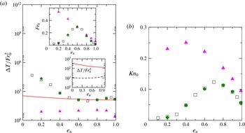
The quantity in (3.9) is called ‘normalized’ excess temperature, which is compared with simulation data in figure 10(a) as a function of
 $e_{n}$
. The corresponding variation of Froude number (3.8) is displayed in the upper inset. The two sets of data, denoted by squares and diamonds, refer to simulations for
 ${\it\nu}_{av}=0.01$
(with
 $W/d=400$
as extracted from figure 9
a) and
 ${\it\nu}_{av}=0.005$
(with
 $W/d=800$
as extracted from figure 9
c) respectively. These simulation data show a good agreement with theory (Rongali & Alam Reference Rongali and Alam2015, unpublished) up to a restitution coefficient of
 $e_{n}=0.5$
, but quantitative agreement worsens for
 $e_{n}<0.5$
. The disagreement for lower values of
 $e_{n}$
can be reconciled from the viewpoint of density inhomogeneities as discussed later in § 3.2.5.
On the other hand, the third data set, denoted by triangles in figure 10(a), which refer to
 ${\it\nu}_{av}=0.005$
(with
 $W/d=400$
as in figure 9
b), deviates considerably from theory for the whole range of
 $e_{n}$
. This might be due to the violation of an inbuilt assumption of the theory as we discuss below.
The variation of the centreline Knudsen number
 $Kn_{0}$
(
 $={\it\lambda}_{0}/W$
) with
 $e_{n}$
is shown in figure 10(b). Note that
 $Kn_{0}$
is of
 $O(0.1)$
or less for two of the data sets (squares and diamonds) and they closely match with each other, with a non-monotonic variation of
 $Kn_{0}$
with
 $e_{n}$
: the Knudsen number is
 $Kn_{0}=0.05$
at
 $e_{n}\rightarrow 1$
, increases to a maximum of
 $Kn_{0}\approx 0.12$
at
 $e_{n}=0.7$
and decreases monotonically with further decrease of
 $e_{n}$
. On the other hand, the data obtained from figure 9(b), denoted by triangles in figure 10(a,b), correspond to
 $Kn_{0}=O(0.1)$
and larger. The disagreement of theory with the latter data set in figure 10(a) is possibly due to the relatively larger values of
 $Kn_{0}$
for all
 $e_{n}$
. Recall that an inbuilt assumption of the theory is
 $Kn_{0}\ll 1$
and
 $Fr_{0}\ll 1$
which is satisfied only for
 $e_{n}\sim 1$
for the first two data sets (squares and diamonds in figure 10
a).
Snapshots of instantaneous particle positions for (a)
 $e_{n}=0.9$
and (b)
 $e_{n}=0.2$
, with other parameters as in figure 9(a). Power spectra of the coarse-grained density fields of (a) and (b) are shown in (c) and (d) respectively.

3.2.5. Possible role of axial inhomogeneities
For the two data sets denoted by squares and diamonds in figure 10(b), the centreline Knudsen number
 $Kn_{0}$
increases initially as
 $e_{n}$
is decreased, reaches a maximum and decreases thereafter. This implies that the granular gas becomes more rarefied around the channel centreline with decreasing
 $e_{n}$
down to
 $e_{n}\approx 0.7$
, before entering into a less-rarefied regime for
 $e_{n}<0.7$
. The critical
 $e_{n}$
at which the above flow transition occurs is in fact tied to clustering of particles along the axial direction as we shall demonstrate below.
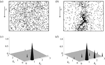
For parameter values as in figure 9(a), snapshots of the system for
 $e_{n}=0.9$
and 0.2 are displayed in figures 11(a) and 11(b) respectively. The particle distribution appears homogeneous at
 $e_{n}=0.9$
, but there are considerable variations along both streamwise and lateral directions at
 $e_{n}=0.2$
. To better characterize the spatial organization of particles, the system is divided into
 $n_{x}\times n_{y}$
cells and the density (the area fraction of particles) is calculated in each cell and is stored as a matrix of size
 $n_{x}\times n_{y}$
from which the power spectrum is calculated using the fast Fourier transform (Liss et al.
Reference Liss, Conway and Glasser2002; Alam et al.
Reference Alam, Chikkadi and Gupta2009). The coefficients,
 $a(k_{x},k_{y})$
, of the Fourier series for the coarse-grained density field,
 $$\begin{eqnarray}a(k_{x},k_{y})\exp [\text{i}2{\rm\pi}(k_{x}x/L+k_{y}y/W)],\end{eqnarray}$$
are found and stored in a matrix
 $\unicode[STIX]{x1D653}$
. The power spectrum (
 $\mathscr{P}$
) of the density field is then calculated from
 $$\begin{eqnarray}\displaystyle \mathscr{P}(k_{x},k_{y})=\frac{2\unicode[STIX]{x1D653}\boldsymbol{\cdot }\text{conj}(\unicode[STIX]{x1D653})}{(n_{x}n_{y})^{2}}, & & \displaystyle\end{eqnarray}$$
which is normalized by the size of the matrix to remove its dependence on the chosen mesh.
Figures 11(c) and 11(d) show the power spectra for
 $e_{n}=0.9$
and 0.2 respectively. There is a dominant peak at
 $(k_{x},k_{y})=(0,1)$
in figure 11(c) which is a signature of the inhomogeneous distribution of particles along the wall-normal (
 $y$
) direction; this is dubbed ‘plug-type’ flow as expected in the Poiseuille flow. On the other hand, at
 $e_{n}=0.2$
, figure 11(d) contains an additional dominant peak at
 $(k_{x},k_{y})=(0,2)$
, along with sub-dominant peaks at
 $(k_{x},k_{y})=(1,0)$
and
 $(1,1)$
. Collectively, the peaks at
 $(k_{x},k_{y})=(0,1)$
and
 $(1,0)$
imply that the particles are inhomogeneously distributed along both the streamwise and wall-normal directions, and is dubbed ‘slug/clump’ flow (Liss et al.
Reference Liss, Conway and Glasser2002; Alam et al.
Reference Alam, Chikkadi and Gupta2009). Therefore, with reference to figure 9(a,c), the flow transitions from plug to slug/clump as the dissipation is increased. These axial inhomogeneities increase the centreline mean-free path
 ${\it\lambda}_{0}$
, leading to a decrease of both
 $Kn_{0}$
and
 $Fr_{0}$
for
 $e_{n}<0.6$
, and are, in turn, responsible for the sharp increase of
 ${\rm\Delta}T/Fr_{0}^{2}$
in the same limit, as illustrated in figure 10(a).
4. Conclusion and discussion
4.1. Conclusion: competition between rarefaction and inelastic dissipation
The roles of inelastic dissipation and wall-roughness in two well-known rarefaction phenomena, the ‘Knudsen-minimum’ effect and the ‘bimodality’ of the temperature profile, have been elucidated for a dilute granular/athermal Poiseuille flow via event-driven simulations of smooth inelastic hard disks under gravity. The wall roughness has a crucial role in the elastic limit (
 $e_{n}\rightarrow 1$
): in channels with smooth walls (
 ${\it\beta}_{w}\sim -1$
, i.e. reflected-type collisions), we uncovered a local minimum in the flow rate (resembling the well-known Knudsen minimum) that occurred at a Knudsen number of
 $Kn\sim O(0.01)$
, but the maximum flow rate occurred at a finite Knudsen number of
 $Kn\sim O(1)$
, beyond which the flow rate decreases. On the other hand, the Knudsen minimum was found to be absent (i) even for quasi-elastic collisions (
 $e_{n}<0.99$
), irrespective of the wall roughness, as well as (ii) for relatively rougher walls (
 ${\it\beta}_{w}>-0.6$
) at any
 $e_{n}$
as summarized in the phase diagram in figure 4(c). An anomalous effect, the decreased slip velocity with increasing
 $Kn$
, was uncovered in smooth-walled channels for dissipative particles, which is responsible for the continual decrease of the flow rate with increasing
 $Kn$
for
 $e_{n}<0.99$
. The origin of this anomalous variation of the slip velocity seems to be tied to the competing effects of (i) the dissipation-induced ‘clustering’ (i.e. the inhomogeneity of the density field along the transverse/wall-normal direction) and (ii) the rarefaction-induced ‘declustering’ of particles along the wall-normal direction.
The granular temperature profile is found to be of ‘bimodal’ shape, with a minimum at the channel centreline and two symmetric maxima away from centre, at any
 $Kn>0$
for
 $e_{n}\leqslant 0.9997$
. In contrast, the temperature bimodality is known to occur in the Poiseuille flow of a molecular gas (
 $e_{n}=1$
) beyond a critical value of
 $Kn>Kn_{c}\sim 0.01$
(Tij & Santos Reference Tij and Santos1994). We found that the origin of temperature bimodality is inelastic dissipation in the continuum limit (i.e. at
 $Kn\sim 0$
), but the rarefaction effects take over beyond
 $Kn>O(0.1)$
as in its molecular counterpart. Therefore, the observed temperature bimodality in granular Poiseuille flow is a consequence of the competition between dissipation and rarefaction as discussed in a phase diagram in the (
 $Kn,1-e_{n}$
)-plane in figure 8. Increasing inelastic dissipation increases the excess temperature ratio
 ${\rm\Delta}T$
(3.4) and hence the degree of temperature bimodality is enhanced. The above finding is at odds with the predictions (
 ${\rm\Delta}T$
decreases with decreasing
 $e_{n}$
from the elastic limit and then increases again) of a kinetic model (Tij & Santos Reference Tij and Santos2004). On the other hand, the simulation results on
 ${\rm\Delta}T$
agree well with the predictions of Rongali & Alam (Reference Rongali and Alam2015, unpublished) as long as the underlying assumptions in the theory (i.e. the inelastic dissipation
 $(1-e_{n})$
, the Knudsen number
 $Kn$
and the Froude number
 $Fr$
must be kept small) are satisfied.


4.2. Discussion: implications for granular hydrodynamic equations
Lastly, we remark on the validity of Navier–Stokes (NS)-order hydrodynamic description for granular gases. With reference to figure 8, the NS equations will hold perfectly in the ‘unimodal’ regime of the phase diagram (to the left of the solid line with circles). On the other hand, we know that the rarefaction-driven bimodality (to the right of the dashed line in figure 8 for
 $Kn>0.01$
) cannot be predicted by NS-equations and requires at least Burnett-order equations. In the region lying between the solid and dashed lines in figure 8, the temperature profile remains bimodal which is, however, driven by inelastic dissipation as discussed in § 3.2.2. In this regime, the NS-equations may hold as long as (i) the Knudsen number
 $Kn$
and (ii) the inelastic dissipation
 $(1-e_{n})$
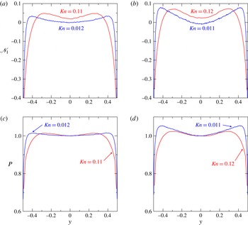
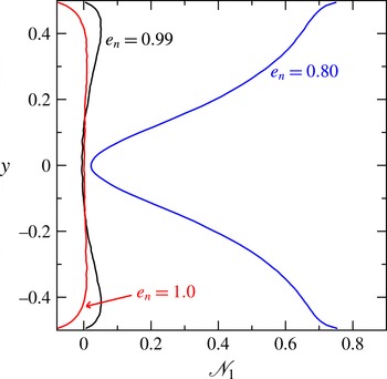
are small. This is because the normal stress difference, which requires a Burnett-order description (Sela & Goldhirsch Reference Sela and Goldhirsch1998; Saha & Alam Reference Saha and Alam2014), becomes finite and measurable with increasing dissipation. This is evident from a comparison between figures 12(a) and 12(b) which display the profiles of scaled first normal stress difference
 $\mathscr{N}_{1}$
, as defined in (A 2), for
 $e_{n}=1$
and
 $0.99$
respectively. Each panel further illustrates that
 $\mathscr{N}_{1}$
increases (in the bulk) with increasing
 $Kn$
for specified values of
 $e_{n}$
.
For a theoretical understanding, let us now consider the transverse momentum equation for the steady, unidirectional flow of a granular fluid:
 $$\begin{eqnarray}\frac{\text{d}p_{yy}}{\text{d}y}=0\equiv \frac{\text{d}p}{\text{d}y}-\frac{1}{2}\frac{\text{d}\mathscr{N}_{1}^{\ast }}{\text{d}y},\end{eqnarray}$$
where
 $\mathscr{N}_{1}^{\ast }=(p_{xx}-p_{yy})$
and
 $p=(p_{xx}+p_{yy})/2$
. For NS-equations,
 $\mathscr{N}_{1}^{\ast }=0$
and hence
 $p(y)$
should be uniform across the channel width. Figure 12(c) confirms that the pressure is nearly uniform in the bulk of the channel (except near boundaries) for
 $Kn=0.012$
and
 $e_{n}=1$
, but visible non-uniformity prevails at higher values of
 $Kn=0.11$
. Recall from figure 8 that the onset of bimodality occurs at
 $Kn=Kn_{c}\approx 0.01$
for
 $e_{n}=1$
, and NS-equations are expected to hold below
 $Kn_{c}$
for this case. On the other hand, figure 12(d) indicates that the pressure is non-uniform for both
 $Kn=0.011$
and 0.12 when the particles are slightly dissipative (
 $e_{n}=0.99$
). The origin of non-uniform pressure at
 $Kn=0.011$
for
 $e_{n}=0.99$
can be tied to the ‘non-negligible’ second term in (4.1) as confirmed from figure 12(b). Therefore, we conclude that, in a phase diagram such as in figure 8, the region of validity of NS-hydrodynamics is indeed small (at least for granular Poiseuille flow).
Future theoretical work should focus on solving the Boltzmann equation with an exact collision kernel, or solving the resultant extended hydrodynamic equations (Saha & Alam Reference Saha and Alam2014) that are valid at least in the Burnett regime. The latter, however, requires the derivation of boundary conditions for higher-order hydrodynamic fields, which can be undertaken in the future too.
Acknowledgements
We sincerely thank Mr R. Rongali for providing the analytical expressions of equations (3.10) and (3.11) for inelastic hard disks. M.A. acknowledges partial funding support from Department of Atomic Energy, Government of India via the DAE-SRC Outstanding Research Investigator Award (DAE/MA/4265).
Appendix A. Granular Poiseuille flow: steady state and hydrodynamic fields
The simulation model for the gravity-driven granular Poiseuille flow, depicted in figure 1(a), consists of a channel of length
 $L$
along the periodic
 $x$
-direction and bounded by two plane rigid frictional walls, parallel to the
 $x$
-direction, with a separation of width
 $W$
(along the
 $y$
-direction), and the gravitational acceleration (
 $g$
) is acting along the
 $x$
-direction. As discussed in § 2.1, the frictional properties of the walls are modelled via a two-parameter model (2.2): (i) the wall-tangential restitution coefficient (
 $-1\leqslant {\it\beta}_{w}\leqslant 1$
) and (ii) the wall-normal restitution coefficient (
 $e_{w}$
) for particle–wall collisions. For all simulations, we set
 $e_{w}=1$
, and the wall roughness is varied by varying the value of
 ${\it\beta}_{w}$
, with
 ${\it\beta}_{w}=-1$
and
 $1$
representing perfectly smooth and rough walls respectively. The collision rule for particle–particle interactions is given by (2.1), with
 $e_{n}$
representing the normal restitution coefficient for particle–particle collisions.
Given the mean density (area fraction) of disks
 ${\it\nu}_{av}$
, the width
 $W$
and the length
 $L$
of the channel, a collection of
 $N$
identical smooth and rigid inelastic disks of mass
 $m=1$
and diameter
 $d=1$
are positioned randomly within the channel, and the disks are assigned random velocities (chosen from a normal distribution). With this initial configuration and wall conditions, the material is allowed to flow under the action of gravity, and an event-driven algorithm (Lubachevsky Reference Lubachevsky1991) is used to simulate the temporal dynamics of this system.
A.1. Steady state and Knudsen number
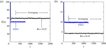
Figure 13(a,b) displays the temporal variations of the total kinetic energy,
 $$\begin{eqnarray}E(t)=\frac{1}{2N}\mathop{\sum }_{i=1}^{N}c_{xi}^{2}+c_{yi}^{2},\end{eqnarray}$$
per particle. The data in figures 13(a) and 13(b) correspond to smooth- (
 ${\it\beta}_{w}=-0.95$
) and rough-walled (
 ${\it\beta}_{w}=0.95$
) channels respectively; other parameters are the same as in figure 2 and listed in table 1. It is seen that
 $E(t)$
fluctuates around some statistical mean value after a transient period, irrespective of the values of
 ${\it\beta}_{w}$
and the mean Knudsen number
 $Kn$
(2.3). In each figure, the initial period of transients continues till a few hundreds of collisions per particle, beyond which the data are collected to calculate hydrodynamic fields and related coarse-grained quantities.


Evolution of kinetic energy, (A 1), versus time for (a)
 ${\it\beta}_{w}=-0.95$
(smooth wall) and (b)
 ${\it\beta}_{w}=0.95$
(rough wall). The system reaches a statistical steady state when
 $E(t)$
fluctuates around some mean value; the vertical line in each panel marks an approximate time at which data is collected for averaging. The mean density is
 ${\it\nu}_{av}=0.01$
and the restitution coefficient is
 $e_{n}=0.9999$
, and the parameter combinations of (
 $W/d,N$
) for different
 $Kn$
are listed in table 1.


For most simulations, we used a mean density (2.4) of
 ${\it\nu}_{av}=0.01$
or less, and the Knudsen number was changed by varying the width of the channel (
 $W/d$
) and the number of particles
 $N$
by keeping the channel length (
 $L/d$
) fixed (Protocol
 $1$
, see § 2.2). Since the hydrodynamic fields vary across the wall-normal direction
 $y$
(see below), the channel is partitioned into a number of bins (
 $n_{bin}$
) parallel to the flow direction
 $x$
, each of width
 $w=W/n_{bin}$
. Table 1 provides details on the system parameters used to vary the average Knudsen number (2.3) as well as the number of bins used for averaging. The ‘bin-wise’ averaging procedure has been described in § 2.2. The two values of
 $Kn$
marked in each panel of figure 13 correspond to different combinations of (
 $W/d,N$
), which are given in table 1.
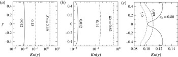
The cross-stream variations of the local Knudsen number
 $Kn(y)$
are shown in figure 14(a–c). In figure 14(a,b), three profiles of
 $Kn(y)$
are plotted for different combinations of (
 $W/d,N$
), resulting in different values of the mean Knudsen number; other parameter values are as in figure 13(a,b). Clearly, the local
 $Kn$
varies along the wall-normal direction, albeit modestly, for both smooth- (figure 14
a) and rough-walled (figure 14
b) channels. The modulations of
 $Kn(y)$
become stronger when the restitution coefficient (
 $e_{n}$
) is decreased, see figure 14(
 $c$
) for which the parameter combinations of (
 $W/d,N$
) were chosen such that
 $Kn=\langle Kn(y)\rangle \approx 0.1$
as in figure 5(b).
A.2. Hydrodynamic profiles in granular Poiseuille flow
For the present system the statistical steady state corresponds to a ‘non-equilibrium’ steady state for which the stream-wise velocity (
 $U$
), volume fraction (
 ${\it\nu}$
) and granular temperature (
 $T$
) remain invariant in time, having spatial variations along the wall-normal direction (
 $y$
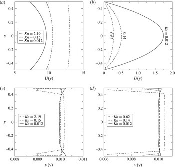
). Typical velocity and density profiles are shown in figure 15 for flows in smooth- (
 ${\it\beta}_{w}=-0.95$
, figure 15
a,c) and rough-walled (
 ${\it\beta}_{w}=0.95$
, figure 15
b,d) channels, with parameter values as in figure 2. As expected, the velocity profiles remain symmetric about the channel centreline
 $y=0$
. It is clear from figure 15(a) that there is a large slip velocity when the channel walls are smooth (
 ${\it\beta}_{w}=-0.95$
), and the magnitude of the slip velocity increases with increasing
 $Kn$
and so does the centreline velocity. In contrast, the slip velocity remains finite but small when the walls are rough (
 ${\it\beta}_{w}=0.95$
, figure 15
b) compared to that for smooth-walled channels; although there is no discernible change in the slip velocity with increasing
 $Kn$
, the centreline velocity (and hence the average velocity as well as the flow rate) decreases markedly with increasing
 $Kn$
. Collectively, figures 15(a) and 15(b) confirm that the slip velocity can be changed from nearly zero to some large value by changing the wall-roughness parameter
 ${\it\beta}_{w}$
from 1 to
 $-1$
.
The density profiles in figure 15(c,d) suggest that the wall-normal variations of density in the ‘bulk’ (around the centreline
 $y=0$
) of the channel remain relatively small (but finite) for both smooth and rough walls for elastic collisions (
 $e_{n}=1.0$
). On the other hand, for a given wall-roughness
 ${\it\beta}_{w}$
, increasing the Knudsen number from the continuum limit (
 $Kn\sim 0$
) to the rarefied regime (
 $Kn\sim O(1)$
) makes the density variation relatively smaller (i.e. more homogeneous) in the bulk of the channel. For a specified
 $Kn$
, increasing the inelastic dissipation (i.e. decreasing
 $e_{n}$
) ensures discernible density modulations across the channel width as discussed in § 3.1 (see figure 5
b in the main text); this is dubbed ‘dissipation-induced’ clustering (see also § A.4).
Profiles of (a,b) the streamwise velocity and (c,d) the density for flows in smooth-walled (
 ${\it\beta}_{w}=-0.95$
, a,c) and rough-walled (
 ${\it\beta}_{w}=0.95$
, b,d) channels. Other parameter values are listed in table 1.

Effect of
 $e_{n}$
on the first normal stress difference,
 $\mathscr{N}_{1}=(p_{xx}-p_{yy})/p$
, at
 $Kn\approx 0.1$
. Other parameters are as in figure 5(b).

A.3. Possible role of normal stress difference on flow rate
It is well-known in rarefied gas dynamics (Kogan Reference Kogan1969) that finite values of Knudsen number (
 $Kn$
) give rise to a non-zero normal stress difference which remains of infinitesimal magnitude in a molecular gas. In contrast, however, the inelastic dissipation makes the normal stress differences (Sela & Goldhirsch Reference Sela and Goldhirsch1998; Saha & Alam Reference Saha and Alam2014) finite and ‘measurable’. This additional effect of inelasticity may have some impact on the macroscopic behaviour of Poiseuille flow (e.g. the mass-flow rate) as we discuss below.
In figure 16, we compare the profiles of the ‘scaled’ first normal stress difference (Chikkadi & Alam Reference Chikkadi and Alam2009; Alam & Luding Reference Alam and Luding2003, Reference Alam and Luding2005a ,Reference Alam, Luding, Garcia-Rojo, Herrmann and McNamara b )
 $$\begin{eqnarray}\mathscr{N}_{1}=\frac{p_{xx}-p_{yy}}{p}=\frac{2(p_{xx}-p_{yy})}{(p_{xx}+p_{yy})}\sim (T_{x}-T_{y}),\end{eqnarray}$$
where
 $p_{ij}=\langle {\it\nu}C_{i}C_{j}\rangle$
and
 $C_{i}$
is the peculiar velocity, see (2.7); the Knudsen number is set to
 $Kn\approx 0.1$
as in the main panel of figure 5(b). It is clear that inelastic dissipation enhances the first normal stress difference across the channel width. Since (A 2) is also a measure of the temperature anisotropy (
 $T_{x}\neq T_{y}$
), this implies that the fluctuation velocity levels along the flow direction are higher than those along the wall-normal direction as dissipation increases. The latter finding may partially be responsible for the enhanced flow rate with increasing dissipation as found in figure 4(a).
A.4. Dissipation versus rarefaction: effects on density profile
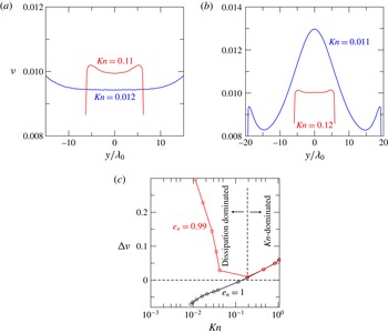
The above issue of dissipation-induced ‘clustering’ (i.e. the density inhomogeneity along the transverse/wall-normal direction) is also evident from a comparison of density profiles in figure 17(a,b). The corresponding temperature profiles are shown in figure 6, see the related discussion on temperature bimodality in § 3.2.1. It is clear from figure 17(a,b) that, for any specified
 $e_{n}$
, increasing the Knudsen number makes the density profiles relatively homogeneous in the ‘bulk’ of the channel; this is dubbed ‘rarefaction-induced’ declustering.
Figure 17(c) displays the variations of the ‘excess’ density at
 $y=0$
(with respect to mean/average density),
 $$\begin{eqnarray}{\rm\Delta}{\it\nu}=\frac{{\it\nu}(0)}{{\it\nu}_{av}}-1,\end{eqnarray}$$
with the Knudsen number
 $Kn$
for two values of the restitution coefficient; here,
 ${\it\nu}(0)$
is the density at the channel centreline and
 ${\it\nu}_{av}$
is the mean density. The curves for both
 $e_{n}=1$
(black circles) and 0.99 (red squares) coincide with each other for
 $Kn\geqslant 0.2$
, implying that dissipation plays no role in the bulk dynamics of density profiles for
 $Kn\geqslant 0.2$
. It is clear that, for
 $e_{n}=1$
, there is a critical Knudsen number of
 $Kn\approx 0.2$
above/below which there is a net accumulation/depletion of particles at
 $y=0$
. Interestingly, even a small amount of dissipation (
 $e_{n}=0.99$
) leads to an overall accumulation of particles (
 ${\rm\Delta}{\it\nu}>0$
) around the channel centreline at any
 $Kn<0.2$
, and the degree of particle accumulation (
 $\propto {\rm\Delta}{\it\nu}$
) increases with decreasing
 $Kn$
for a given
 $e_{n}\neq 1$
. Further decreasing the restitution coefficient (not shown) increases the value of the excess density
 ${\rm\Delta}{\it\nu}$
at
 $Kn<0.2$
. Based on these results, we conclude that the inelastic dissipation has a primary influence on the hydrodynamic density profiles at lower values of
 $Kn$
. The vertical dashed line in figure 17(c) approximately demarcates the regions of ‘dissipation-dominated’ and ‘rarefaction-dominated’ flows.
Profiles of density for (a)
 $e_{n}=1.0$
and (b)
 $e_{n}=0.99$
, with parameter values as in figure 6. (c) Variation of the excess density,
 ${\rm\Delta}{\it\nu}=({\it\nu}(0)/{\it\nu}_{av}-1)$
, with Knudsen number.