


Introduction
Soil freezing in cold areas is connected with a complex of physical, chemical and mechanical processes. The relief of these regions is formed and transformed by different geo-cryological phenomena: thermokarst, pingos, formation and melting of underground ice lenses and hypersaline underground zones. Study of pingo formation requires the modelling of temperature fields, heat-transfer properties, moisture and chemical properties of the soil. Soil is a porous medium consisting of a mineral crystalline structure, ice, constrained water, salt solution and a gas component (air with water vapour). Physical and mechanical soil properties are sensitive to the mineral composition and the size of mineral particle of skeleton due to different specific surfaces of particles (fine and coarse granularity). The specific surfaces of a particle define the quantity of the water in pore space. Chemical composition and granularity define the temperature of the phase transition. Soil heaving can be divided into seasonal and long-term parts. This process can be accompanied by pingo formation. The height and rate of growth of a pingo and velocity formation depend on soil type, moisture content, granularity and salinity. The thickness of the upper freezing layer and the freezing rate play an important role, and are determined by the variability of climatic conditions. The soil-heaving process depends on moisture migration to the phase boundary.
The mathematical model is based on the hypothesis that the process is caused by two interlinked processes. The first is the formation of an area with high salt concentration in front of the phase boundary, caused by salt being forced out of the freezing soil. The second is osmotic phenomena in finegrained soil. Such soils have a small diffusion coefficient, so a soil layer can play the role of a semi-permeable membrane. As soil freezes, the difference in salt concentration between the zone in front of the phase boundary and remote soil increases. Osmotic pressure tries to equalize the chemical potentials of solution and porous water. This pressure can reach large values: in a Siberian pingo a pressure of about 52 atm was measured (Reference FrenzelFrenzel, 1973). These processes cause water migration to the phase boundary and the increase in osmotic pressure. Ice segregation and pingo origin has been studied by many researchers, some of whom have studied the osmotic mechanism of underground ice growth (Reference GoldsteinGoldstein, 1948; Reference Guseva, Grigoryan and KrassGuseva, 1986, Reference Guseva1987; Reference Grigoryan, Krass, Guseva and GevorkyanGrigoryan and others, 1987, Reference Grigoryan, Krass, Guseva and Gevorkyan1989; Reference Horiguchi and NakanoHoriguchi and Nakano, 1993). The mathematical model of pingo formation includes heat transfer, diffusion and filtration, equations for an increase in soil volume for different freezing regimes, the equation for water flux to the phase boundary, the criteria of different freezing regimes and an equation for a solution interlayer, and is based on previous work (Reference Guseva, Grigoryan and KrassGuseva, 1986, Reference Guseva1987; Reference Grigoryan, Krass, Guseva and GevorkyanGrigoryan and others, 1987, Reference Grigorian, Guseva and Krass1989).
During the freezing of the unfrozen soil, the chemical content of the salt solution can be divided into three parts: the first part stays in the frozen soil, the second falls as a solid residual and the last is transported to the liquid phase of the unfrozen soil. One result of these processes is the formation of hypersaline underground zones. Salt concentration in these areas can reach ≥ 200gL-1 . Such brine zones cannot be frozen (Reference ErshovErshov, 1982).
Characteristics of the different soils
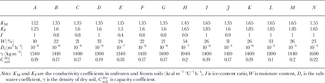
Analysis of pingo formation demonstrates three regimes of soil freezing:
-
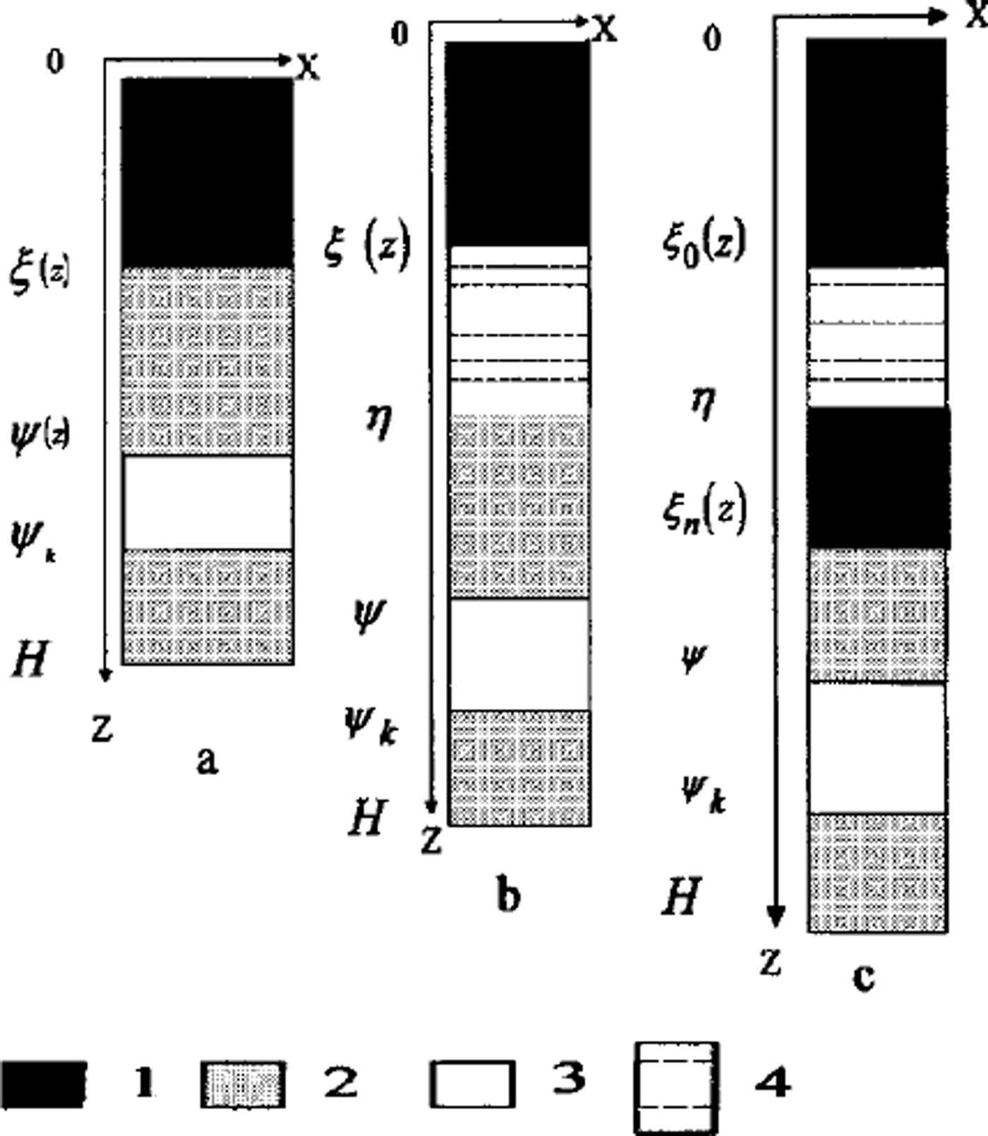
(1) The first regime arises when the osmotic pressure is less than the weight of soil over the phase boundary. There is no water migration. This regime is realized in two cases: at a soil depth and at low salt concentration in front of the phase boundary. Osmotic pressure increases due to growth concentration near the phase boundary (Fig. 1a).
-
(2) When the osmotic pressure equals the weight of frozen soil above the phase boundary the second regime is initiated. The water flows to a phase boundary due to differences of salt concentration. The phase boundary moves fast enough and this water is frozen quasi-homogeneously If the water-migration rate exceeds the rate of freezing, a layer of free water appears between the frozen and unfrozen soil (Fig. 1b).
-
(3) The third regime is characterized by the origination of the water layer. This salinity layer brakes the movement of the phase boundary. Soil under this layer can be frozen due to further freezing. Another phase boundary is formed. A water layer between two phase boundaries can be locked in and be frozen later (Fig. 1c).
Two-dimensional schema of area D: (a) regime 1; (b) regime 2; (c) regime 3 1. Frozen soil; 2. unfrozen soil; 3 water-bearing horizon; 4. brine layer.
The mathematical model takes into account the heterogeneity of soil through coefficients of heat capacity conductivity and salt diffusion, soil density, total quantity of moisture in soil, quantity of constrained water and quantity of residual salinity in soil.
Mathematical model of soil heaving by freezing process
A two-dimensional area D = (0 ≤ x ≤ r 0, 0 ≤ z ≤ Ψ ≤ H) is considered (Fig. la). The origin of the vertical axis z = 0 is defined at a ground surface with the equation of surface relief z = f(x). Beyond the phase boundary ξ, soil is frozen, and under ξ soil is unfrozen. The boundary between soil and the water-bearing horizon is z = Ψ The water layer appears due to the further soil freezing (the boundary z = η is a low boundary of the underground brine layer). The lower part of the area D is a water-bearing horizon (lower than z = Ψ ) . We assume that water migration is negligible in frozen soil, and a rate of water migration to the phase boundary j = 0 in frozen soil (z ≤ £(*)). The temperature in D is calculated from:

where T is temperature, t is time, Ki ,Ci and Cw are the coefficients of heat conductivity and capacity in melting (i = M) and frozen (i = F) soil and in water, respectively, and W(T) is the volumetric coefficient of moisture content in unfrozen soil.
The equation of salt diffusion in unfrozen soil (z > £(x)) with salt transfer due to water migration to the phase boundary is:

where Cs is salt concentration and Ds is the salt diffusion coefficient in soil.
Boundary conditions exist for Equations (1) and (2):
-
1. On the top surface of the soil, z = f(x), the following conditions apply:

where Ta(x,t) is the air temperature (with correction for radiation) and R* is the resistance of snow cover in winter or vegetation cover in summer. (If R*=0,then T = Ta.)
-
2. There is geothermal flux at the bottom of area z = H and soil concentration:
-
3. On the vertical boundaries, the heat and salt flux are absent and the conditions are:
-
4. At the phase boundary, the Stefan condition for Equation (1) is:
where a is the specific heat of phase transition, 7 is the density of dry soil, Wf is the proportion of unfrozen water in soil at negative temperature, p is the water density, ∂/ ∂n is normal derivative and Kg = [1 + (∂ξ/∂x)2 + (∂ξ/∂z)2]1/2. At the beginning of soil freezing (regime 1), the coefficients are A = 1 and B = 0; in regime 2, A = 1 and B = 1; and in regime 3, ,4 = 0 and B = l.


At the phase boundary, the mass-balance conditions for Equation (2) are:


where j = 0 in regime 1. Water is moved to the phase boundary under pressure, caused by a difference between hydrostatic and osmotic pressure. If the hydrostatic pressures are equal, the water moves to the area with the largest concentration. This process continues while the hydrostatic and osmotic pressures are equalized. Using Darcy’s equation j=–DW(p*–pg), where P* is the difference between the hydrostatic and osmotic pressures, the continuity condition Vj = 0 with boundary conditions at the boundaries of A we can define the effective pressure P* for water moving to the phase boundary and we can write the equation in area z ≥ ξ(x) for the definition of water flux j :

where Dw is a filtration coefficient in unfrozen soil, R is the universal gas constant, Ms is the molecular salt weight, Tk is the temperature on the Kelvin scale and P0 is water pressure in the water-bearing horizon. The conditions of water-layer appearance are: condition dΨ/df ≥ dξ/df, t=t1 defines a time of appearance; condition dψ/dt > dξ/dt, t= t 1 defines the moving of the lower boundary of the water layer; and condition η(t) = η 1 + ψ(t) – ψ(t 1) is the initial condition.
Initial conditions for Equations (1) and (2) are
The increase in soil volume due to freezing is defined by:


where ε is a coefficient of volume increasing due to water-ice phase transition.
The hydrostatic pressure is smaller than the weight of overlying soil (regime 1) and j = O. The soil volume increases due to water flux to the phase boundary (regime 2). The small water inclusions transform into small lenses due to fast phase-boundary movement. The increase in soil volume (regime 3) occurs due to water flux to the salinity water layer.There are regime transition criteria:

where the osmotic pressure PM is defined by the equation


A phase-boundary position can be defined by the condition

where Tp is a phase-transition temperature.
The appearance of a new phase boundary ξ = & in an area with low salt concentration (the area is below the phase boundary) can be estimated from the following temperature condition:

The salinity layer with thickness d(x) = rj ― & is closed and a new boundary ξn is established; & is the old phase boundary. A new salt-accumulation process is started in front of the new boundary ξo due to its movement (see Fig. 1). The temperature T(x, z) and phase boundary ξ are defined from the heat problem (Equation (1)) with Stefan’s boundary condition, and concentration is defined from the diffusion problem (Equation (2)). The geometry of these salinity interlayers depends on relief geometry, soil-heat coefficients and salt-concentration distribution. The mathematical model uses a narrow phase boundary in Stefan’s problem. The thickness of the phase-transition zone is narrow in coarse-grained soils. In fine-grained soils this zone can be wide and consists of both phases of ice: liquid with salt and solid-phase ice.
Numerical Modeling
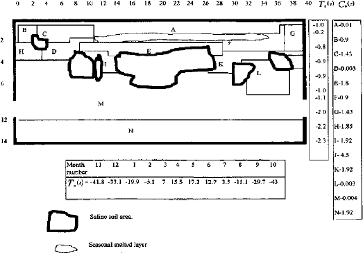
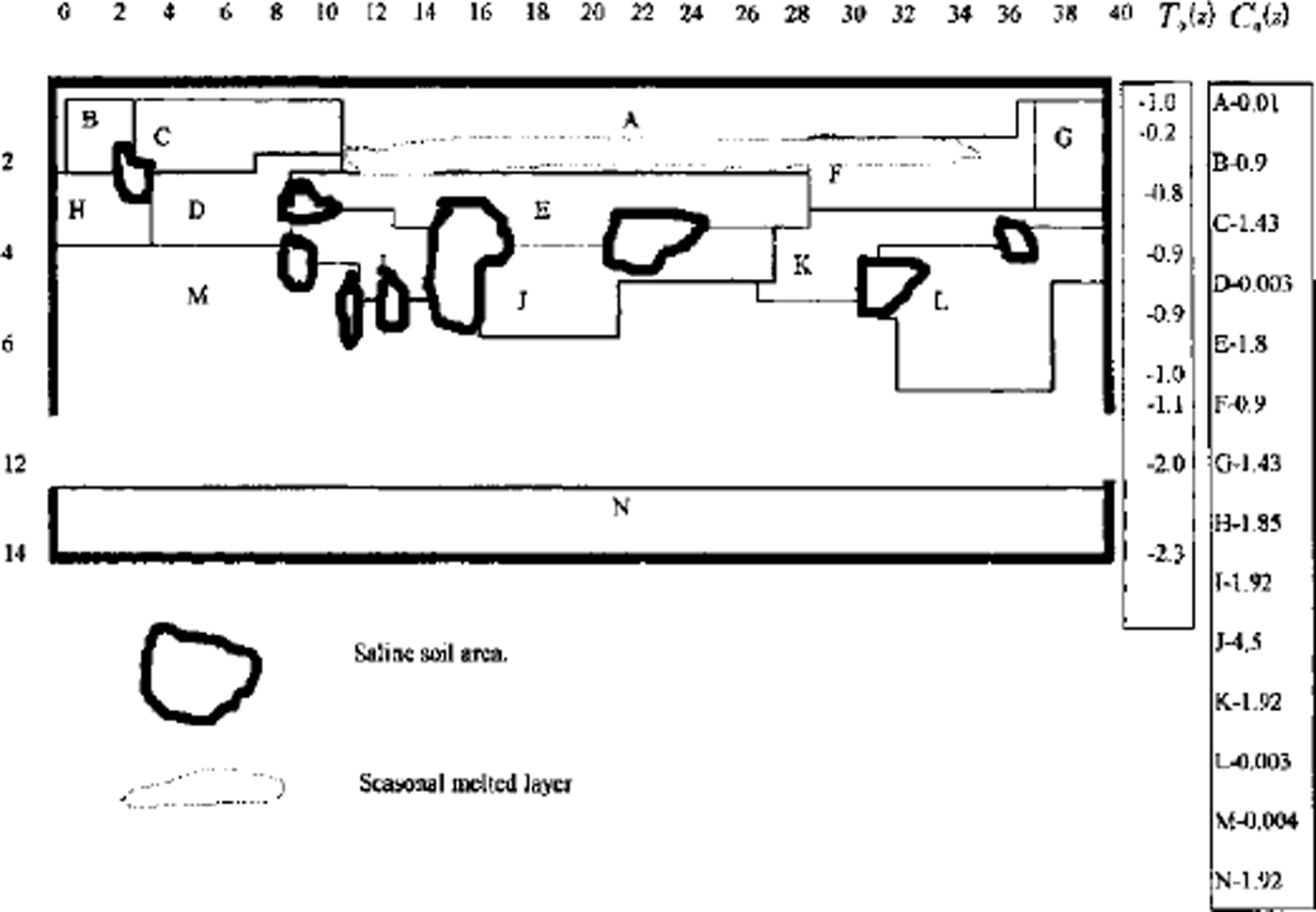
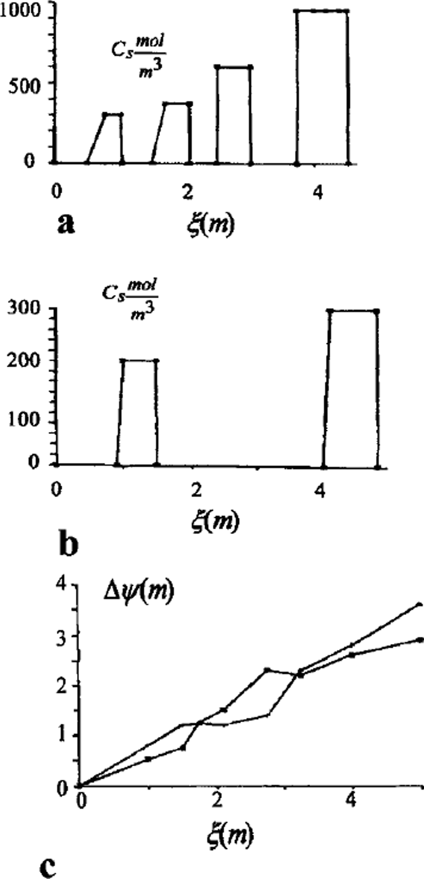
A full model was used for one- and two-dimensional case computations. A finite-difference balance method of smoothing coefficients throughout the computing area was used as numerical model (Reference Guseva, Grigoryan and KrassGuseva 1986, Reference Guseva1987). For numerical simulations a real area with complex distribution of the different lithologies (A-N) was chosen (Fig. 2). There is no connection with the water-bearing horizon in this area. This example is interesting due to closed salt-zones migration during calculation time. The lithologies all have different salinity, heat, moisture and diffusion coefficients. The underground water always contains dissolved salts such as sodium chloride, potassium chloride, calcium sulfate and calcium chloride. The amounts vary, but most solutions range from the salinity of sea water (3.5% dissolved solids by weight) to about ten times that of sea water. A hydrothermal solution is therefore brine (Reference Skinner and PorterSkinner and others, 1992). Initial profiles of the temperature and concentration are shown in Figure 2. The air temperature was changed every month, and the model was run for 20 years. A salinity zone between A and E appeared due to seasonal melting-freezing processes. Salt migrated to this zone from zone E with larger salt concentration than zone A. The salt distribution and stability of this zone is very sensitive to the movement of phase boundaries. Freezing of the seasonal melted layer in winter and the rise of the lower phase boundary define an evolution of this zone. Seasonal soils can be characterized by the periodic migration of this zone due to large temperature gradients. At the soil depth brine zones are left unfrozen. Salt concentration increases there. The volume of these zones is reduced by further freezing of the area (see Figs 2 and 3). Some of them are divided into smaller zones. A connection between lithology boundaries and brine zones is visible (see Figs 2 and 3). Horizontal ice layering with heterogeneity distribution of the horizontal mineral impurities is often observed in permafrost areas. These ice horizons are deposited near the boundary between sand and clay deposits (Reference Kudryavtsev, Poltev, Romanovskiy, Kondratyeva, Melamed and GaraguliaKudryavtsev and others, 1981). Figure 4a and b show salt concentration distributions in water layers, and Figure 4c shows changes of the layer thickness with depth. The initial salt concentration in porous water was Cs = 200 molnr3. The average summer temperature was Ts = 5°C, and the average winter temperatures were Tw = –10°C (Fig. 4a) and Tw = –20°C (Fig. 4b). The salt concentrations and layer thickness increase with depth. The salt accumulation begins after freezing, with the movement of a new phase boundary. The thickness of frozen soil is due to water flux to the phase boundary. The number of brine layers is larger in Figure 4a than in Figure 4b. Interlayers grow better due to slower freezing rates. The water flows more slowly as a phase boundary in Figure 4b. The water here is distributed in volume quasi-uniformly in the form of small inclusions. The total value of frost heaving is defined by the salt concentration in front of the phase boundary, the freezing rate, diffusion and the permeability of the soil for water and salts. Figure 4c shows a computing heaving parameter ( A Ψ = Ψ(t) ― *(0)) as a function of the freezing depths in Figure 4a and b. The total thickness is larger in Figure 4b than in Figure 4a.
Vertical profile of the heterogeneous area for numerical simulation. A-JVare indexes of different types of soil. T0 (Z) is initial vertical temperature distribution. Cs0(Z) is initial concentration distribution in lithological zones A-K The numerical net is irregular: in horizontal direction Δxz = 4m for i= 1–12 and i = 26–40; Axz = 2mfori = 13–25; in vertical direction Δzi = I m for i = 1, 21. Td(t) is the long-term temperature of air at the soil surface. Frozen area with air temperature Ta (t) during t=7years.
Vertical profile of the heterogeneous area for numerical simulation. A-N are indexes of different types of soil. Freeze of area with air temperature Ta(t) during t = 25years.
Salt-concentration distribution of interior soil in salt layers, (a) Soil freezing with summer Ts = 5°C and winter Tw = –10°C temperatures; (b) soil freezing with summer Ts = 5° C and winter Tw=-20° C temperatures; (c) heaving of soil as a function of freezing depth (phase boundary depth).
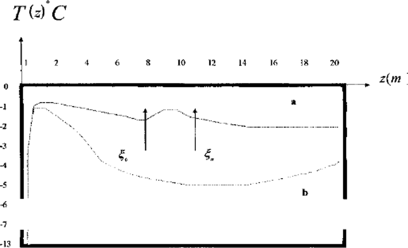
Computations show that the volume of the frozen part rises faster in regime 2 (small lenses) than in regime 3 (larger layers). The sequence of ice-lens growth is in accordance with the texture classification of fine-grained frozen soils (Reference ShumskiyShumskiy, 1955). Unfrozen zones with high concentration are often observed at the underground boundaries. These zones are resistant to heat flux and decrease the rate of freezing. Figure 5 shows a temperature profile of the soil with and without the unfrozen zone (Figs 2 and 3).
Two vertical profiles of temperature in area D: temperature distribution in frozen soil; temperature distribution in soil with thaw brine layer. ξ0 and η = & are phase boundaries.
Discussion
Pingo formation is connected with freezing of taliks and occurs in peatbogs. The total moisture of such soils can reach 40–60% and exceed total soil moisture in the thawing state. Sources of the water which migrates to the phase boundary and forms ice kernels are the initial soil moisture, water from water-bearing horizons with good permeability and water from thaw swamps around the pingo. Long-term pingos usually appear in the area of thermokarst degradation (the last stage). Pingos can reach heights of 30–40 m and have a diameter of about 100–200 m (Reference FrenzelFrenzel, 1973). Pingo formation is accompanied by heaving of the soil surface. In winter, snow is blown from the surface. Vegetation disappears through further reduction of soil temperature (Reference Kudryavtsev, Poltev, Romanovskiy, Kondratyeva, Melamed and GaraguliaKudryavtsev and others, 1981). Bare soil is exposed to deflation. Deflation takes place only where little or no vegetation exists and where loose rock particles are fine enough to be picked up by the wind. Deflation lowers the land surface slowly and irregularly. Deflation varies from a long-term average rate of erosion of a few centimeters per millennium to lm or more within only a few years (Reference Skinner and PorterSkinner and Porter, 1992). Deflation is a reason for the exposure of soil with ice or ice layers. Bare ice melts due to summer heat flux. Snow cover isolates the ground from winter cold flux. These processes lead to degradation of pingo and to crater formation at its upper surface. Water from ice lenses evaporates or flows out. The thermokarst process begins in the case of water-layer appearance at the upper surface (Reference Grigoryan, Guseva and KrassGrigoryan and others, 1983,Reference Grigoryan, Krass, Guseva and Gevorkyan1987; Reference Guseva, Grigoryan and KrassGuseva, 1983). A dome is formed in the center of this crater because the upper load decreases through deflation and melting. External slopes of pingo are frozen while vegetation there is retained, preventing thawing in summer. The change of the processes thermokarst-soil heaving-pingo-thermokarst has a cyclical character.
Conclusion
The approach described explains the following effects: the extent of this process in fine-grained soils; the appearance and formation of ice lenses with a horizontal orientation; the decreasing ice quantity and the appearance of ice lenses with depth; and the existence of an underground boundary above which the ice content in soil is high.



