1 Introduction
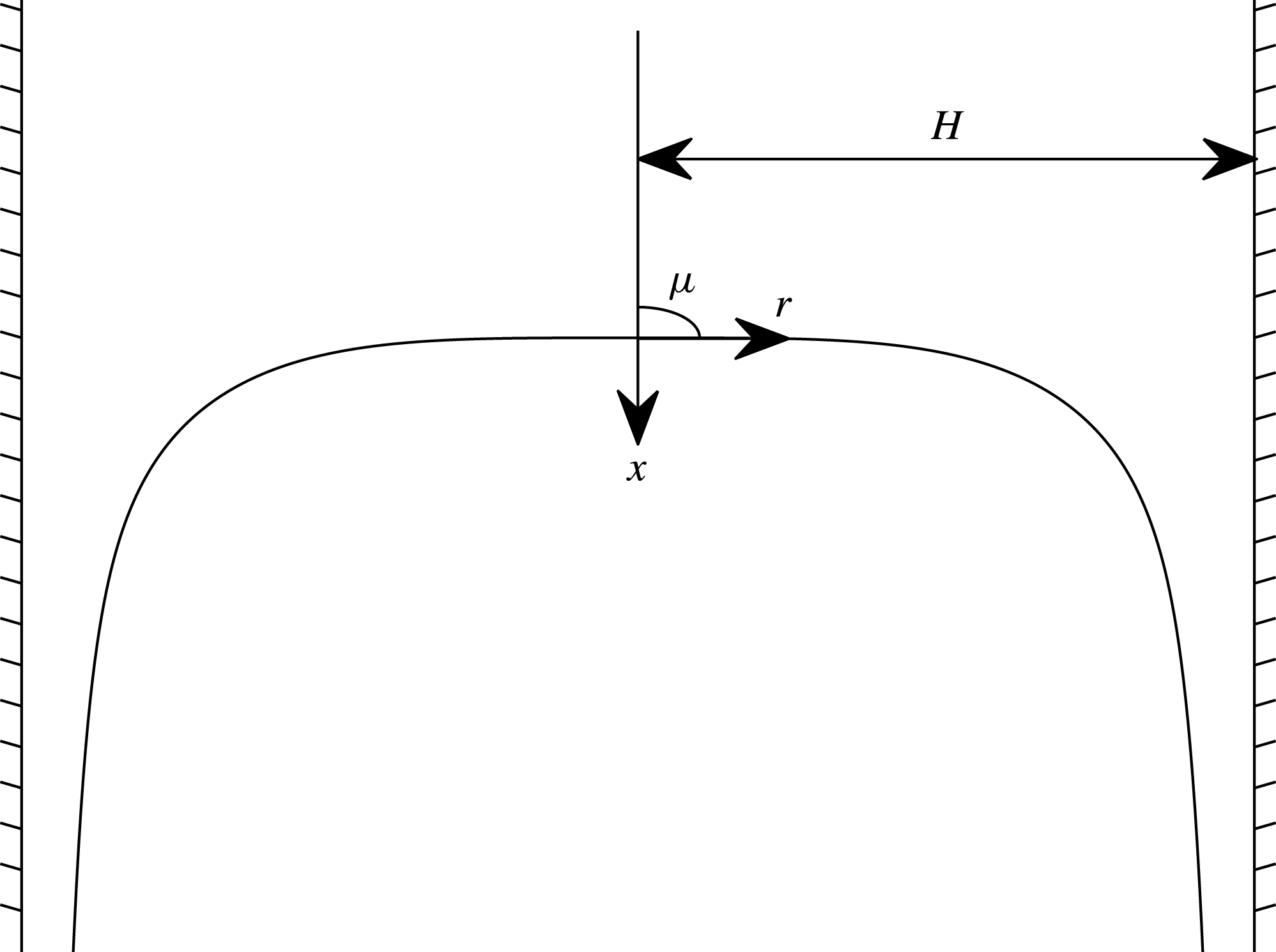
We consider the classical problem of a long bubble rising in a cylindrical tube (see figure 1). Since the experiments of Dumitrescu (Reference Dumitrescu1943), it has been known that large volumes of air can rise steadily through a denser medium in the form of a finger-shaped bubble. This unchanging headform has a radius close to that of the tube, such that there is a thin jet of fluid around the outer edges of the finger. Such bubbles are often referred to as Taylor bubbles. Many authors have performed experiments on this type of flow, in both channel geometry (Collins Reference Collins1965; Maneri & Zuber Reference Maneri and Zuber1974), frequently referred to as plane bubbles, and axisymmetric geometry (most famously Davies & Taylor Reference Davies and Taylor1950; Zukoski Reference Zukoski1966, and for a review, Viana et al. Reference Viana, Pardo, Yanez, Trallero and Joseph2003).
It has been found that the rise velocity
 $U$
is independent of both the length of the bubble and viscous effects, under the condition that the Reynolds number
 $Re$
, given by
 $Re=\unicode[STIX]{x1D70C}HU/\unicode[STIX]{x1D707}$
, is sufficiently large (
 $Re>200$
). Here,
 $\unicode[STIX]{x1D70C}$
and
 $\unicode[STIX]{x1D707}$
are the density and dynamic viscosity of the fluid through which the bubble is travelling and
 $H$
the tube radius. This justifies an inviscid and infinite model, in which we take the bubble to extend indefinitely down the tube. We take the density of air to be negligible compared to that of the heavier fluid, which we assume to be incompressible. Due to the inviscid nature of the problem, we consider the flow to be irrotational.
The problem is characterised by two dimensionless constants, the Froude number,
 $$\begin{eqnarray}\displaystyle & \displaystyle F=\frac{U}{\sqrt{gH}}, & \displaystyle\end{eqnarray}$$
and the Weber number
 $$\begin{eqnarray}\displaystyle & \displaystyle \unicode[STIX]{x1D6FC}=\frac{U^{2}H\unicode[STIX]{x1D70C}}{T}, & \displaystyle\end{eqnarray}$$
where
 $g$
is the acceleration of gravity, and
 $T$
the surface tension.
In this paper, we consider a regime characterised by negligible surface tension. It has been found in experiments that, for a given Weber number, the Froude number is uniquely determined. Therefore, one would hope that the mathematical model described in this paper emits a unique solution
 $F$
when surface tension is neglected. However, this is known not be the case. A unique zero surface tension solution cannot be obtained without the inclusion of surface tension in the equations. Below, we describe the solution space of the two-dimensional Taylor bubbles, and the solution selection procedure.
Formulation of the problem in the
 $(x,r)$
space.

Two-dimensional Taylor bubbles have been the subject of many investigations, where most authors make use of conformal mapping techniques. Denoting
 $\unicode[STIX]{x1D707}$
as the angle between the central streamline and the free surface (see figure 1), we define smooth bubbles as those with
 $\unicode[STIX]{x1D707}=\unicode[STIX]{x03C0}/2$
. Bubbles with
 $\unicode[STIX]{x1D707}=\unicode[STIX]{x03C0}$
are called cusped bubbles, while solutions with any other value of
 $\unicode[STIX]{x1D707}$
we refer to as pointed bubbles. In experiments, cusped and pointed bubbles are never seen, so such solutions are considered non-physical. Garabedian (Reference Garabedian1957) demonstrated analytically that, for
 $T=0$
, smooth plane bubble solutions are not uniquely defined in
 $F$
, but instead there exists a continuum
 $F\in (0,F_{C})$
for which such solutions exist. Using a heuristic energy argument, he claimed the only physically significant solution is the one given by
 $F=F_{C}$
, and found that
 $F_{C}>0.334$
. Vanden-Broeck (Reference Vanden-Broeck1984a
) later showed numerically that
 $F_{C}\approx 0.51$
. He confirmed that all solutions with
 $F<F_{C}$
are smooth bubbles, and furthermore showed that solutions with
 $F>F_{C}$
are cusped bubbles. Modi (Reference Modi1985) and Garabedian (Reference Garabedian1985) both stated there could also exist zero surface tension pointed bubbles with
 $\unicode[STIX]{x1D707}=2\unicode[STIX]{x03C0}/3$
. Such a solution does exist, and was found by Vanden-Broeck (Reference Vanden-Broeck1986), who showed that
 $F=F_{C}$
is the only value for which this is the case.
Taking non-zero values of surface tension, Vanden-Broeck (Reference Vanden-Broeck1984b
) found that, for a given values of
 $\unicode[STIX]{x1D6FC}$
, there exists an infinite discrete set of smooth bubbles
 $F_{1}(\unicode[STIX]{x1D6FC}),F_{2}(\unicode[STIX]{x1D6FC}),\ldots$
. These solutions are bounded above by
 $F^{\ast }\approx 0.318$
, and it was found that as
 $\unicode[STIX]{x1D6FC}\rightarrow \infty$
, these solution branches collapsed to the value
 $F^{\ast }$
. This mechanism, by which a unique solution
 $F^{\ast }$
to the
 $T=0$
problem is found by including surface tension in the system, and then taking the limit as surface tension goes to zero, is called solution selection. A similar mechanism was used to select a unique solution for viscous Saffman–Taylor fingering (McLean & Saffman Reference McLean and Saffman1981). It is known to be associated with exponentially small terms of surface tension (Vanden-Broeck Reference Vanden-Broeck1992). This challenged Garabedian’s claim that the physically significant solution was the
 $F=F_{C}$
solution, since the experimental value for negligible surface tension is given by
 $F_{e}\approx 0.35$
(Collins Reference Collins1965).
It has long been believed that the solutions for the axisymmetric problem exhibit the same behaviour. Levine & Yang (Reference Levine and Yang1990) computed axisymmetric Taylor bubbles using a boundary integral method. They showed that for
 $T=0$
, there again exists a continuum of solutions
 $F\in (0,F_{C})$
for which the bubble is smooth. It was found that
 $F_{C}\approx 0.7$
. In this paper, we show the solution for
 $F=F_{C}$
is a pointed bubble with an interior angle of approximately
 $130^{\circ }$
(i.e.
 $\unicode[STIX]{x1D707}\approx 115^{\circ }$
). Similar to the two-dimensional problem,
 $F=F_{C}$
is the only value for which we find pointed bubbles with zero surface tension. A local behaviour at the apex of this solution is given by Garabedian (Reference Garabedian1985), which we make use of when computing this bubble. The inclusion of surface tension again reduces the continuous set of smooth bubbles to an infinite discrete set
 $F_{1},F_{2},\ldots .$
Levine & Yang computed
 $F_{1}(\unicode[STIX]{x1D6FC})$
, and showed that
 $F_{1}(\unicode[STIX]{x1D6FC})\rightarrow F^{\ast }\approx 0.49$
as
 $1/\unicode[STIX]{x1D6FC}\rightarrow 0$
. This is in excellent agreement with experiments: Viana et al. (Reference Viana, Pardo, Yanez, Trallero and Joseph2003), making use of data collected from a wide selection of previously performed experiments, obtain the experimental value
 $F_{e}\approx 0.48$
. Levine & Yang also computed a small number of solutions on the branches
 $F_{2}$
and
 $F_{3}$
, but did not compute solutions on these branches for small surface tension. In this paper, we present a numerical scheme capable of computing solutions on the higher-order branches
 $F_{2}(\unicode[STIX]{x1D6FC}),F_{3}(\unicode[STIX]{x1D6FC}),\ldots .$
We were unable to compute solutions for
 $\unicode[STIX]{x1D6FC}>160$
. Despite this, similarities between the two-dimensional and axisymmetric solution spaces lead us to conjecture that these higher-order solution branches approach
 $F^{\ast }$
as
 $1/\unicode[STIX]{x1D6FC}\rightarrow 0$
. The numerical scheme presented could prove useful in solving a variety of other axisymmetric problems.
The formulation of the problem follows a numerical approach to solving axisymmetric flows first proposed by Woods (Reference Woods1951), and later independently by Jeppson (Reference Jeppson1970). We map the flow domain to an infinite strip by taking the velocity potential
 $\unicode[STIX]{x1D719}$
and Stokes streamfunction
 $\unicode[STIX]{x1D713}$
as independent variables. We then discretise the space and solve the equations via finite differences. This formulation has been used for a variety of problems (see Brennen Reference Brennen1969; Vanden-Broeck, Miloh & Spivack Reference Vanden-Broeck, Miloh and Spivack1998; Blyth & Părău Reference Blyth and Părău2014). Due to the stagnation point singularity at the apex of the bubble, a solution with the same local behaviour as the bubble at the singular point is derived and a function splitting procedure, previously adopted by a variety of authors (Southwell Reference Southwell1946; Woods Reference Woods1953; Brennen Reference Brennen1966), is used to allow for accurate approximation of derivatives.
The paper is organised as follows. In § 2, we formulate the problem. In § 3, we present a finite difference scheme used to solve the problem for smooth bubbles, along with an explanation of the function splitting procedure used to regulate the singularity at the apex of the bubble. In § 4, we present results for the smooth bubbles. In § 5, we describe a method used to compute the
 $F=F_{C}$
axisymmetric bubble. Section 6 is a conclusion of the paper.
2 Formulation
Consider an axisymmetric bubble rising vertically with constant velocity
 $U$
through a fluid at rest in a tube of radius
 $H$
. We take standard cylindrical coordinates
 $(x,\unicode[STIX]{x1D703},r)$
, where we choose
 $x$
to point in the direction of gravity, and
 $r\in [0,H]$
to be the radial distance from the central streamline
 $r=0$
. We take the origin to be at the apex of the bubble and to travel with the bubble such that the problem is steady. In this frame of reference, the background flow at
 $x\rightarrow -\infty$
is a uniform stream in the positive
 $x$
direction with velocity
 $U$
. We take
 $H$
as the reference length and
 $U$
as the reference velocity. The formulation in the
 $(x,r)$
space is shown in figure 1.
We consider incompressible, inviscid and irrotational flow. Therefore, there exists a velocity potential
 $\unicode[STIX]{x1D719}$
and stokes streamfunction
 $\unicode[STIX]{x1D713}$
given by
 $$\begin{eqnarray}\displaystyle & \displaystyle u=\unicode[STIX]{x1D719}_{x}=\frac{\unicode[STIX]{x1D713}_{r}}{r},\quad v=\unicode[STIX]{x1D719}_{r}=-\frac{\unicode[STIX]{x1D713}_{x}}{r}, & \displaystyle\end{eqnarray}$$
where
 $u$
and
 $v$
are the velocities in the
 $x$
and
 $r$
directions respectively, and subscripts denote partial differentiation. Without loss of generality, we take
 $\unicode[STIX]{x1D719}=0$
at the apex and
 $\unicode[STIX]{x1D713}=0$
on the free surface. Integration of (2.1) at
 $x\rightarrow -\infty$
gives
 $$\begin{eqnarray}\displaystyle & \displaystyle \unicode[STIX]{x1D713}\rightarrow \frac{r^{2}}{2}\quad \text{as}\,x\rightarrow -\infty . & \displaystyle\end{eqnarray}$$
Therefore, the wall is given by
 $\unicode[STIX]{x1D713}=1/2$
. Unlike the two-dimensional streamfunction, the Stokes streamfunction does not satisfy the Laplace equation. This means the powerful tools of complex analysis used to solve the two-dimensional analogue of this problem are unavailable.
On the free surface, as well as
 $\unicode[STIX]{x1D713}=0$
, we must satisfy the Bernoulli equation. This is given by
 $$\begin{eqnarray}\displaystyle & \displaystyle q^{2}-\frac{2}{F^{2}}x+\frac{2}{\unicode[STIX]{x1D6FC}}K=\text{const.}, & \displaystyle\end{eqnarray}$$
where
 $q$
is the magnitude of the velocity,
 $F$
and
 $\unicode[STIX]{x1D6FC}$
are given by (1.1) and (1.2) and
 $K=R_{1}^{-1}+R_{2}^{-1}$
is the mean curvature of the free surface, where the principle radii of curvature,
 $R_{1}$
and
 $R_{2}$
, are counted positive when the centres of curvature lie inside the fluid.
Even though the mapping from the
 $(r,x)$
to the
 $(\unicode[STIX]{x1D719},\unicode[STIX]{x1D713})$
space is not conformal, we still find the mapping beneficial. The domain in the
 $(\unicode[STIX]{x1D719},\unicode[STIX]{x1D713})$
space is the infinite strip
 $\unicode[STIX]{x1D6FA}_{\unicode[STIX]{x1D719}}=\{\unicode[STIX]{x1D713}\in [0,1/2],-\infty <\unicode[STIX]{x1D719}<\infty \}$
. The approach to the problem follows the work of Woods (Reference Woods1951). We seek
 $r$
as a function of the independent variables
 $(\unicode[STIX]{x1D719},\unicode[STIX]{x1D713})$
. The key benefit to working in the potential space as opposed to the physical space is that the free surface is fixed to the positive
 $\unicode[STIX]{x1D719}$
-axis (
 $\unicode[STIX]{x1D713}=0,\unicode[STIX]{x1D719}>0$
).
The mapping from the
 $(x,r)$
to the
 $(\unicode[STIX]{x1D719},\unicode[STIX]{x1D713})$
space produces the relations
 $$\begin{eqnarray}\displaystyle & \displaystyle x_{\unicode[STIX]{x1D719}}=\frac{1}{2}f_{\unicode[STIX]{x1D713}},\quad x_{\unicode[STIX]{x1D713}}=-\frac{f_{\unicode[STIX]{x1D719}}}{2f}, & \displaystyle\end{eqnarray}$$
where
 $f=r^{2}$
. Woods derived a governing equation for
 $f(\unicode[STIX]{x1D719},\unicode[STIX]{x1D713})$
, given by
 $$\begin{eqnarray}\displaystyle \frac{f_{\unicode[STIX]{x1D719}\unicode[STIX]{x1D719}}}{f}-\left(\frac{f_{\unicode[STIX]{x1D719}}}{f}\right)^{2}+f_{\unicode[STIX]{x1D713}\unicode[STIX]{x1D713}}=0. & & \displaystyle\end{eqnarray}$$
Furthermore, it can be shown that
 $$\begin{eqnarray}\displaystyle & \displaystyle q=2\left(\frac{f_{\unicode[STIX]{x1D719}}^{2}}{f}+f_{\unicode[STIX]{x1D713}}^{2}\right)^{-1/2}, & \displaystyle\end{eqnarray}$$
 $$\begin{eqnarray}\displaystyle & \displaystyle K=-\frac{f_{\unicode[STIX]{x1D713}}q}{2\sqrt{f}}+\frac{q^{3}}{4\sqrt{f}}\left[f_{\unicode[STIX]{x1D713}}f_{\unicode[STIX]{x1D719}\unicode[STIX]{x1D719}}-f_{\unicode[STIX]{x1D719}}f_{\unicode[STIX]{x1D719}\unicode[STIX]{x1D713}}-\frac{1}{2}\frac{f_{\unicode[STIX]{x1D713}}f_{\unicode[STIX]{x1D719}}^{2}}{f}\right]. & \displaystyle\end{eqnarray}$$
Making use of (2.4), we find it beneficial to differentiate Bernoulli’s equation (2.3) with respect to
 $\unicode[STIX]{x1D719}$
in order to remove the
 $x$
term. This gives us
 $$\begin{eqnarray}\displaystyle & \displaystyle qq_{\unicode[STIX]{x1D719}}-\frac{1}{2F^{2}}f_{\unicode[STIX]{x1D713}}+\frac{1}{\unicode[STIX]{x1D6FC}}K_{\unicode[STIX]{x1D719}}=0. & \displaystyle\end{eqnarray}$$
The boundary conditions on the central streamline and the wall
 $f=1$
can be written as
 $$\begin{eqnarray}\displaystyle & \displaystyle f(\unicode[STIX]{x1D719},0)=0\quad \unicode[STIX]{x1D719}<0, & \displaystyle\end{eqnarray}$$
 $$\begin{eqnarray}\displaystyle & \displaystyle f(\unicode[STIX]{x1D719},1/2)=1\quad \forall \unicode[STIX]{x1D719}, & \displaystyle\end{eqnarray}$$
respectively. Finally, (2.2) gives us the upstream condition
 $$\begin{eqnarray}\displaystyle f\rightarrow 2\unicode[STIX]{x1D713}\quad \text{as}\,\unicode[STIX]{x1D719}\rightarrow -\infty . & & \displaystyle\end{eqnarray}$$
This completes the formulation of the problem. It is left to find
 $f$
as a function of the independent variables
 $(\unicode[STIX]{x1D719},\unicode[STIX]{x1D713})$
such that it satisfies (2.5), (2.8), (2.9), (2.10) and (2.11).
For the two-dimensional problem, we take standard Cartesian coordinates
 $(x,y)$
, where again
 $x$
points downwards and
 $y$
is the coordinate orthogonal with gravity (analogous to
 $r$
in the axisymmetric problem, figure 1). In this case, since the mapping from the physical to potential space is conformal,
 $y$
satisfies the Laplace equation in the
 $(\unicode[STIX]{x1D719},\unicode[STIX]{x1D713})$
space. Furthermore, a similar formula to (2.8) can be obtained in terms of
 $y(\unicode[STIX]{x1D719},\unicode[STIX]{x1D713})$
.
In the following section, we will present a finite difference scheme used to solve this system.
3 Finite difference scheme
We truncate the infinite strip
 $\unicode[STIX]{x1D6FA}_{\unicode[STIX]{x1D719}}$
to a finite domain
 $\unicode[STIX]{x1D6FA}_{T}=\{\unicode[STIX]{x1D713}\in [0,1/2],\unicode[STIX]{x1D719}\in [-\unicode[STIX]{x1D719}_{1},\unicode[STIX]{x1D719}_{2}]\}$
, where
 $\unicode[STIX]{x1D719}_{1}$
and
 $\unicode[STIX]{x1D719}_{2}$
are positive real numbers. We must ensure when computing our solutions that we truncate far enough both up- and downstream such that the solution becomes invariant to truncating the domain further. This is explained in greater detail in § 4.
We found it beneficial to perform two coordinate transforms,
 $$\begin{eqnarray}\displaystyle \unicode[STIX]{x1D719}=\left\{\begin{array}{@{}ll@{}}-s^{2},\quad & \text{if}\,\unicode[STIX]{x1D719}<0,\\ s^{2},\quad & \text{if}\,\unicode[STIX]{x1D719}\geqslant 0,\end{array}\right. & & \displaystyle\end{eqnarray}$$
 $$\begin{eqnarray}\displaystyle \unicode[STIX]{x1D713}=t^{2}, & & \displaystyle\end{eqnarray}$$
 $$\begin{eqnarray}\displaystyle & \displaystyle f_{\unicode[STIX]{x1D713}}=\frac{1}{2t}f_{t}, & \displaystyle\end{eqnarray}$$
 $$\begin{eqnarray}\displaystyle & \displaystyle f_{\unicode[STIX]{x1D713}\unicode[STIX]{x1D713}}=\frac{1}{4t^{2}}\left(f_{tt}-\frac{f_{t}}{t}\right), & \displaystyle\end{eqnarray}$$
 $\unicode[STIX]{x1D719}$
. We discretise
 $\unicode[STIX]{x1D6FA}_{T}$
with
 $M$
points in
 $s$
and
 $N$
points in
 $t$
as follows:
 $$\begin{eqnarray}\displaystyle \left.\begin{array}{@{}ll@{}}s_{i}=-Ah+(i-1)h & i=1,\ldots ,M,\\[2.0pt] \displaystyle t_{j}=\frac{1}{\sqrt{2}}\frac{j-1}{N-1} & j=1,\ldots ,N,\end{array}\right\} & & \displaystyle\end{eqnarray}$$
where
 $A<M$
is a positive integer, chosen such that there are sufficient points upstream and downstream. From (3.3), we can see that
 $$\begin{eqnarray}\displaystyle \unicode[STIX]{x1D719}_{1}=\left(Ah\right)^{2},\quad \unicode[STIX]{x1D719}_{2}=\left((M-A-1)h\right)^{2}. & & \displaystyle\end{eqnarray}$$
This choice of discretisation produces
 $MN$
unknowns:
 $f$
evaluated at each mesh point
 $f(s_{i},t_{j})=f_{i,j}$
. Therefore, we require
 $MN$
equations. We note that the mesh points are uniformly spaced in
 $s$
and
 $t$
with differences
 $$\begin{eqnarray}\displaystyle \left.\begin{array}{@{}l@{}}\unicode[STIX]{x0394}s=s_{i+1}-s_{i}=h,\\ \displaystyle \unicode[STIX]{x0394}t=t_{j+1}-t_{j}=\frac{1}{\sqrt{2}}\frac{1}{N-1}=k.\end{array}\right\} & & \displaystyle\end{eqnarray}$$
We will impose an equation at each mesh point. In all interior nodes, we apply the governing equation (2.5). We apply the boundary condition (2.11) at
 $\unicode[STIX]{x1D719}=-\unicode[STIX]{x1D719}_{1}$
. This is an approximation, since the boundary condition should be applied in the limit
 $\unicode[STIX]{x1D719}\rightarrow -\infty$
, but it is found that the error is negligible given
 $\unicode[STIX]{x1D719}_{1}$
is sufficiently large, as discussed in § 4. We apply the wall and free-surface boundary conditions at their respective places on the mesh. The full discrete system of equations is given by
 $$\begin{eqnarray}\displaystyle \displaystyle \frac{\unicode[STIX]{x2202}^{2}f_{i,j}}{\unicode[STIX]{x2202}\unicode[STIX]{x1D713}^{2}}+\frac{\unicode[STIX]{x2202}^{2}f_{i,j}}{\unicode[STIX]{x2202}\unicode[STIX]{x1D719}^{2}}/f_{i,j}-\left[\frac{\unicode[STIX]{x2202}f_{i,j}}{\unicode[STIX]{x2202}\unicode[STIX]{x1D719}}/f_{i,j}\right]^{2} & = & \displaystyle 0\quad \text{for}\left\{\begin{array}{@{}l@{}}i=2,\ldots ,M,\quad \\ j=2,\ldots ,N-1,\quad \end{array}\right.\end{eqnarray}$$
 $$\begin{eqnarray}\displaystyle \displaystyle f_{i,N}-1 & = & \displaystyle 0\quad \text{for}\,i=1\ldots M,\end{eqnarray}$$
 $$\begin{eqnarray}\displaystyle \displaystyle f_{1,j}-2\unicode[STIX]{x1D713}_{j} & = & \displaystyle 0\quad \text{for}\,j=1\ldots N,\end{eqnarray}$$
 $$\begin{eqnarray}\displaystyle \displaystyle f_{i,1} & = & \displaystyle 0\quad \text{for}\,i=1\ldots A+1,\end{eqnarray}$$
 $$\begin{eqnarray}\displaystyle \displaystyle q_{i,1}\frac{\unicode[STIX]{x2202}q_{i,1}}{\unicode[STIX]{x2202}\unicode[STIX]{x1D719}}-\frac{1}{2F^{2}}\frac{\unicode[STIX]{x2202}f_{i,1}}{\unicode[STIX]{x2202}\unicode[STIX]{x1D713}}+\frac{1}{\unicode[STIX]{x1D6FC}}\frac{\unicode[STIX]{x2202}K_{i,1}}{\unicode[STIX]{x2202}\unicode[STIX]{x1D719}} & = & \displaystyle 0\quad \text{for}\,i=A+2\ldots M,\end{eqnarray}$$
 $K_{i,1}$
refer to values of the curvature (2.7) computed at the mesh point
 $(\unicode[STIX]{x1D719}_{i},\unicode[STIX]{x1D713}_{1})$
. All the derivatives (
 $f_{s}$
,
 $f_{t}$
etc.) are approximated using second-order central difference formulae or, when necessity dictates, second-order one-sided formulae. We then use formulae such as (3.2a
)–(3.2b
) to obtain values of
 $f_{\unicode[STIX]{x1D713}},f_{\unicode[STIX]{x1D713}\unicode[STIX]{x1D713}}$
(etc.) at each mesh point. We note that these formulae cannot be used for derivatives where
 $s=0$
or
 $t=0$
. In such cases, we approximate the derivatives directly in
 $\unicode[STIX]{x1D719}$
and
 $\unicode[STIX]{x1D713}$
. This system of
 $MN$
equations can be solved for the
 $MN$
unknowns using Newton’s method. We terminate the iterations in Newton’s method once the
 $L^{\infty }$
-norm of the residuals (values on the right-hand side of equations (3.6a
–3.6e
)) is of order
 $10^{-12}$
. Once we have obtained values of
 $f_{i,j}$
for all
 $(i,j)$
, we can obtain values of
 $x_{i,j}$
by integrating (2.4) along lines of constant
 $\unicode[STIX]{x1D713}$
. This is given by
 $$\begin{eqnarray}\displaystyle & \displaystyle x_{i+1,j}=x_{i,j}+\frac{1}{2}\int _{\unicode[STIX]{x1D719}_{i}}^{\unicode[STIX]{x1D719}_{i+1}}\frac{\unicode[STIX]{x2202}f}{\unicode[STIX]{x2202}\unicode[STIX]{x1D713}}(\unicode[STIX]{x1D719},\unicode[STIX]{x1D713}_{j})\,\text{d}\unicode[STIX]{x1D719}. & \displaystyle\end{eqnarray}$$
The above integral is approximated via the trapezoidal rule.
3.1 Singularity removal: smooth bubbles
It is found that singularities, when not properly accounted for, cause inaccuracies to the approximation of derivatives in finite difference schemes (Woods Reference Woods1953). In particular, as mesh spacing is decreased, the inaccuracies grow and the method fails to converge in the limit as mesh spacing goes to zero. In our case, we must remove the singularity associated with the stagnation point at the apex of the bubble
 $\unicode[STIX]{x1D719}=\unicode[STIX]{x1D713}=0$
. Woods (Reference Woods1953) derived a function splitting procedure to regulate singularities in finite difference methods, paying particular attention to Poisson’s equation. We follow a similar strategy, but with some modifications. In particular, while Woods performs the function splitting to the differential operator of the governing equation as a whole, we instead use the method on individual partial derivatives, due to the nonlinearity of (2.5).
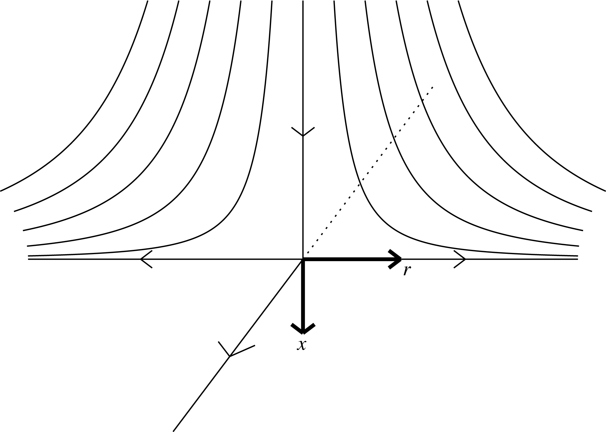
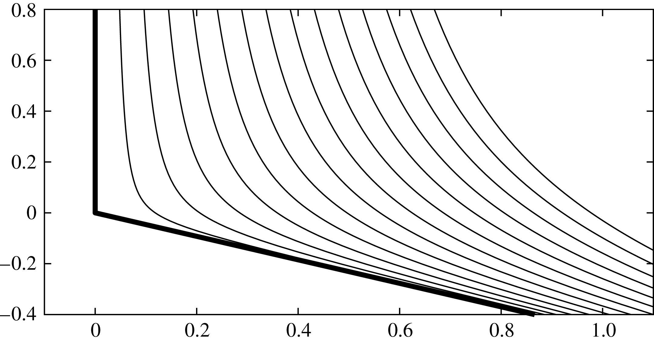
Axisymmetric flow onto a plate parallel with the
 $r$
-axis. Some streamlines are shown.

The basic procedure to regulate the singularity is to first consider some function
 $f=\unicode[STIX]{x1D712}(\unicode[STIX]{x1D719},\unicode[STIX]{x1D713})$
which has the same singular behaviour as our flow at the singularity and satisfies the governing equation. A natural choice is the flow onto an infinite flat plate (see figure 2). The velocity potential and streamfunction of this flow are found to be
 $$\begin{eqnarray}\displaystyle \unicode[STIX]{x1D719}=B\left({\textstyle \frac{1}{2}}f-x^{2}\right),\quad \unicode[STIX]{x1D713}=-Bfx, & & \displaystyle\end{eqnarray}$$
where
 $B$
is an arbitrary positive constant. This can be re-arranged to remove
 $x$
, producing a cubic for
 $f$
. The unique real positive root of this cubic,
 $\unicode[STIX]{x1D712}=f$
, is given by
 $$\begin{eqnarray}\displaystyle \unicode[STIX]{x1D712} & = & \displaystyle \frac{2}{3B}\unicode[STIX]{x1D719}+\frac{1}{B^{2/3}}\left(A\unicode[STIX]{x1D719}^{3}+\unicode[STIX]{x1D713}^{2}+\unicode[STIX]{x1D713}\sqrt{2A\unicode[STIX]{x1D719}^{3}+\unicode[STIX]{x1D713}^{2}}\right)^{1/3}\nonumber\\ \displaystyle & & \displaystyle +\,\frac{1}{B^{2/3}}\left(A\unicode[STIX]{x1D719}^{3}+\unicode[STIX]{x1D713}^{2}-\unicode[STIX]{x1D713}\sqrt{2A\unicode[STIX]{x1D719}^{3}+\unicode[STIX]{x1D713}^{2}}\right)^{1/3},\end{eqnarray}$$
where
 $A=8/(27B)$
. This function can be differentiated to analytically compute values of
 $\unicode[STIX]{x1D712}_{\unicode[STIX]{x1D719}}$
(etc.) everywhere in the flow domain. The unknown constant
 $B$
can be used to match the flow configuration in figure 2 to our problem by satisfying
 $$\begin{eqnarray}\displaystyle & \displaystyle \unicode[STIX]{x1D712}(\unicode[STIX]{x1D719}_{i},\unicode[STIX]{x1D713}_{j})-f(\unicode[STIX]{x1D719}_{i},\unicode[STIX]{x1D713}_{j})=0, & \displaystyle\end{eqnarray}$$
for some mesh point
 $(\unicode[STIX]{x1D719}_{i},\unicode[STIX]{x1D713}_{j})$
in the flow close to the singularity. A natural choice is to use the mesh point on the free surface immediately after the apex,
 $(\unicode[STIX]{x1D719}_{A+2},\unicode[STIX]{x1D713}_{1})=(h^{2},0)$
. This gives rise to
 $$\begin{eqnarray}\displaystyle & \displaystyle B=2\frac{\unicode[STIX]{x1D719}_{A+2}}{f_{A+2,1}}. & \displaystyle\end{eqnarray}$$
We then re-write our solution
 $f$
as
 $$\begin{eqnarray}\displaystyle f(\unicode[STIX]{x1D719},\unicode[STIX]{x1D713})=(f-\unicode[STIX]{x1D712})+\unicode[STIX]{x1D712}. & & \displaystyle\end{eqnarray}$$
The motivation for subtracting and adding
 $\unicode[STIX]{x1D712}$
is now we can numerically compute derivatives on the function
 $(f-\unicode[STIX]{x1D712})$
and analytically compute the derivatives of
 $\unicode[STIX]{x1D712}$
. Hence, in our code, the values of
 $\unicode[STIX]{x2202}f_{i,j}/\unicode[STIX]{x2202}\unicode[STIX]{x1D719}$
are computed as
 $$\begin{eqnarray}\displaystyle & \displaystyle \frac{\unicode[STIX]{x2202}f_{i,j}}{\unicode[STIX]{x2202}\unicode[STIX]{x1D719}}=\unicode[STIX]{x1D6FF}_{\unicode[STIX]{x1D719}}(f_{i,j}-\unicode[STIX]{x1D712}_{i,j})+\frac{\unicode[STIX]{x2202}\unicode[STIX]{x1D712}_{i,j}}{\unicode[STIX]{x2202}\unicode[STIX]{x1D719}}, & \displaystyle\end{eqnarray}$$
where
 $\unicode[STIX]{x1D6FF}_{\unicode[STIX]{x1D719}}$
is some finite difference approximation of the derivative. Since
 $\unicode[STIX]{x1D712}$
has been defined such that it has the same behaviour as
 $f$
at the stagnation point, the function
 $(f-\unicode[STIX]{x1D712})$
is not singular, allowing us to approximate derivatives via finite differences. Furthermore, since we have an explicit formula (3.9) for
 $\unicode[STIX]{x1D712}$
, computing derivatives (for example,
 $\unicode[STIX]{x2202}\unicode[STIX]{x1D712}_{i,j}/\unicode[STIX]{x2202}\unicode[STIX]{x1D719}$
) is possible analytically. Therefore, (3.13) can be used to approximate derivatives at all mesh points. We note that this would not work on a nonlinear differential operator, say
 $(\unicode[STIX]{x2202}f_{i,j}/\unicode[STIX]{x2202}\unicode[STIX]{x1D719})^{2}$
, since in this case
 $$\begin{eqnarray}\displaystyle & \displaystyle \left[\frac{\unicode[STIX]{x2202}(f_{i,j}-\unicode[STIX]{x1D712}_{i,j}+\unicode[STIX]{x1D712}_{i,j})}{\unicode[STIX]{x2202}\unicode[STIX]{x1D719}}\right]^{2}\neq \left[\frac{\unicode[STIX]{x2202}(f_{i,j}-\unicode[STIX]{x1D712}_{i,j})}{\unicode[STIX]{x2202}\unicode[STIX]{x1D719}}\right]^{2}+\frac{\unicode[STIX]{x2202}\unicode[STIX]{x1D712}_{i,j}}{\unicode[STIX]{x2202}\unicode[STIX]{x1D719}}^{2}. & \displaystyle\end{eqnarray}$$
However, one can simply apply (3.13), and then square the result to obtain the required value. Brennen (Reference Brennen1966) followed a similar method to remove a stagnation point singularity in a successive relaxation scheme used to compute axisymmetric cavitating flow past an obstruction in a tunnel. He solved the same governing equation (2.5) but with different boundary conditions. He approximated the front stagnation point using non-cavitating flow past a disc or sphere. However, he treated the governing equation as though it were linear as an approximation. Although this dramatically reduces computational time and requirements on storage (you can avoid computing terms like
 $\unicode[STIX]{x2202}\unicode[STIX]{x1D712}_{i,j}/\unicode[STIX]{x2202}\unicode[STIX]{x1D719}$
at all interior mesh points, since
 $\unicode[STIX]{x1D712}$
is chosen to satisfy the governing equation), in this paper, such an approximation is unnecessary.
Special care must be taken when computing the integral (3.7) through the stagnation point. For example, consider the case where
 $i=A$
and
 $j=1$
, such that the integral is on the streamline
 $\unicode[STIX]{x1D713}=0$
, from the point
 $\unicode[STIX]{x1D719}_{A}=-h^{2}$
to
 $\unicode[STIX]{x1D719}_{A+1}=0$
. If we attempt to approximate the integral using the trapezoidal rule, taking into account (3.13), we obtain
 $$\begin{eqnarray}\displaystyle & \displaystyle \int _{-h^{2}}^{0}\frac{\unicode[STIX]{x2202}f}{\unicode[STIX]{x2202}\unicode[STIX]{x1D713}}\,\text{d}\unicode[STIX]{x1D719}\approx \frac{h^{2}}{2}\left[\unicode[STIX]{x1D6FF}_{\unicode[STIX]{x1D713}}(f_{A+1,1}-\unicode[STIX]{x1D712}_{A+1,1})+\unicode[STIX]{x1D6FF}_{\unicode[STIX]{x1D713}}(f_{A,1}-\unicode[STIX]{x1D712}_{A,1})+\frac{\unicode[STIX]{x2202}\unicode[STIX]{x1D712}_{A+1,1}}{\unicode[STIX]{x2202}\unicode[STIX]{x1D713}}+\frac{\unicode[STIX]{x2202}\unicode[STIX]{x1D712}_{A,1}}{\unicode[STIX]{x2202}\unicode[STIX]{x1D713}}\right]. & \displaystyle\end{eqnarray}$$
However, the value of
 $\unicode[STIX]{x2202}\unicode[STIX]{x1D712}_{A+1,1}/\unicode[STIX]{x2202}\unicode[STIX]{x1D713}$
is singular. Instead of directly applying the trapezoidal rule, we must integrate the
 $\unicode[STIX]{x2202}\unicode[STIX]{x1D712}/\unicode[STIX]{x2202}\unicode[STIX]{x1D713}$
term explicitly, that is,
 $$\begin{eqnarray}\displaystyle & \displaystyle \int _{-h^{2}}^{0}\frac{\unicode[STIX]{x2202}y}{\unicode[STIX]{x2202}\unicode[STIX]{x1D713}}\,\text{d}\unicode[STIX]{x1D719}\approx \frac{h^{2}}{2}\left[\unicode[STIX]{x1D6FF}_{\unicode[STIX]{x1D713}}(y_{A+1,1}-\unicode[STIX]{x1D712}_{A+1,1})+\unicode[STIX]{x1D6FF}_{\unicode[STIX]{x1D713}}(y_{A,1}-\unicode[STIX]{x1D712}_{A,1})\right]+\int _{-h^{2}}^{0}\frac{\unicode[STIX]{x2202}\unicode[STIX]{x1D712}}{\unicode[STIX]{x2202}\unicode[STIX]{x1D713}}\,\text{d}\unicode[STIX]{x1D719}, & \displaystyle\end{eqnarray}$$
where the second term is an integral calculated analytically. The same consideration must be made when integrating from
 $\unicode[STIX]{x1D719}_{A+1}=0$
to
 $\unicode[STIX]{x1D719}_{A+2}=h^{2}$
for
 $\unicode[STIX]{x1D713}=0$
.
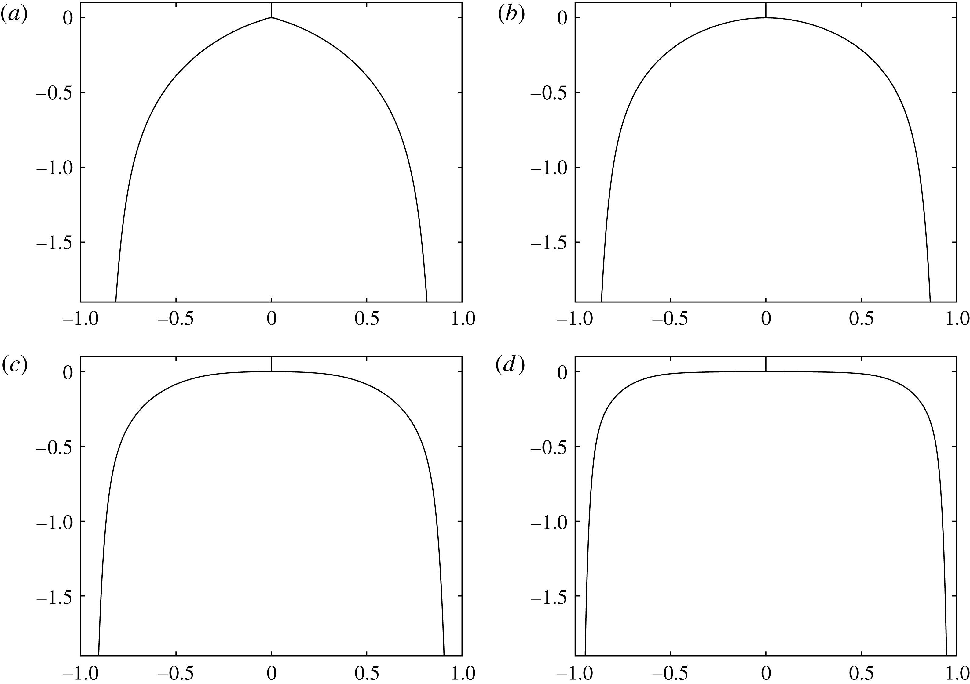
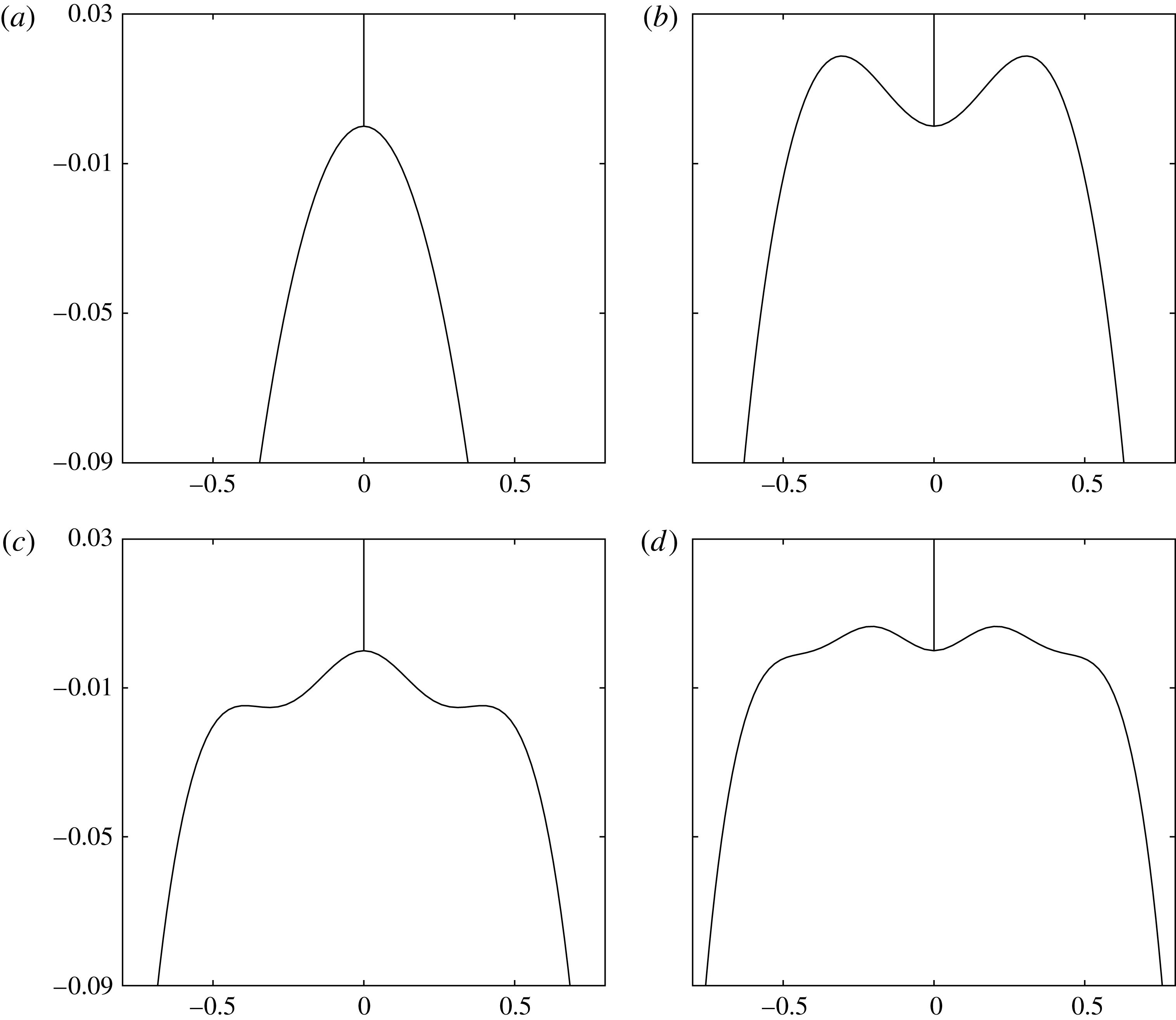
Various profiles of axisymmetric bubbles for the zero surface tension case with Froude numbers (a)
 $F=0.65$
, (b)
 $F=0.5$
, (c)
 $F=0.35$
and (d)
 $F=0.2$
.

It is of interest to note that Vanden-Broeck (Reference Vanden-Broeck1991) constructed a similar finite difference scheme for this problem, taking
 $r$
as a function of the independent variables
 $(x,\unicode[STIX]{x1D713})$
. However, the method took no measures to regulate the singularity at the stagnation point. Repeating the numerical scheme, the authors found the results satisfactory for crude meshes but ultimately diverge with mesh refinement. On the other hand, we found the new numerical scheme described above convergent upon mesh refinement, at least as far as computationally practical, as shown in § 4.
We feel it worth mentioning for completeness that, to remove the singularity in the two-dimensional problem, we used the classical solution of flow in a right-angled corner, given by
 $$\begin{eqnarray}\displaystyle y=\unicode[STIX]{x1D712}(\unicode[STIX]{x1D719},\unicode[STIX]{x1D713})=\text{Im}\Big\{\frac{\text{i}}{B}\sqrt{\unicode[STIX]{x1D719}+\text{i}\unicode[STIX]{x1D713}}\Big\}. & & \displaystyle\end{eqnarray}$$
4 Results for smooth Taylor bubbles
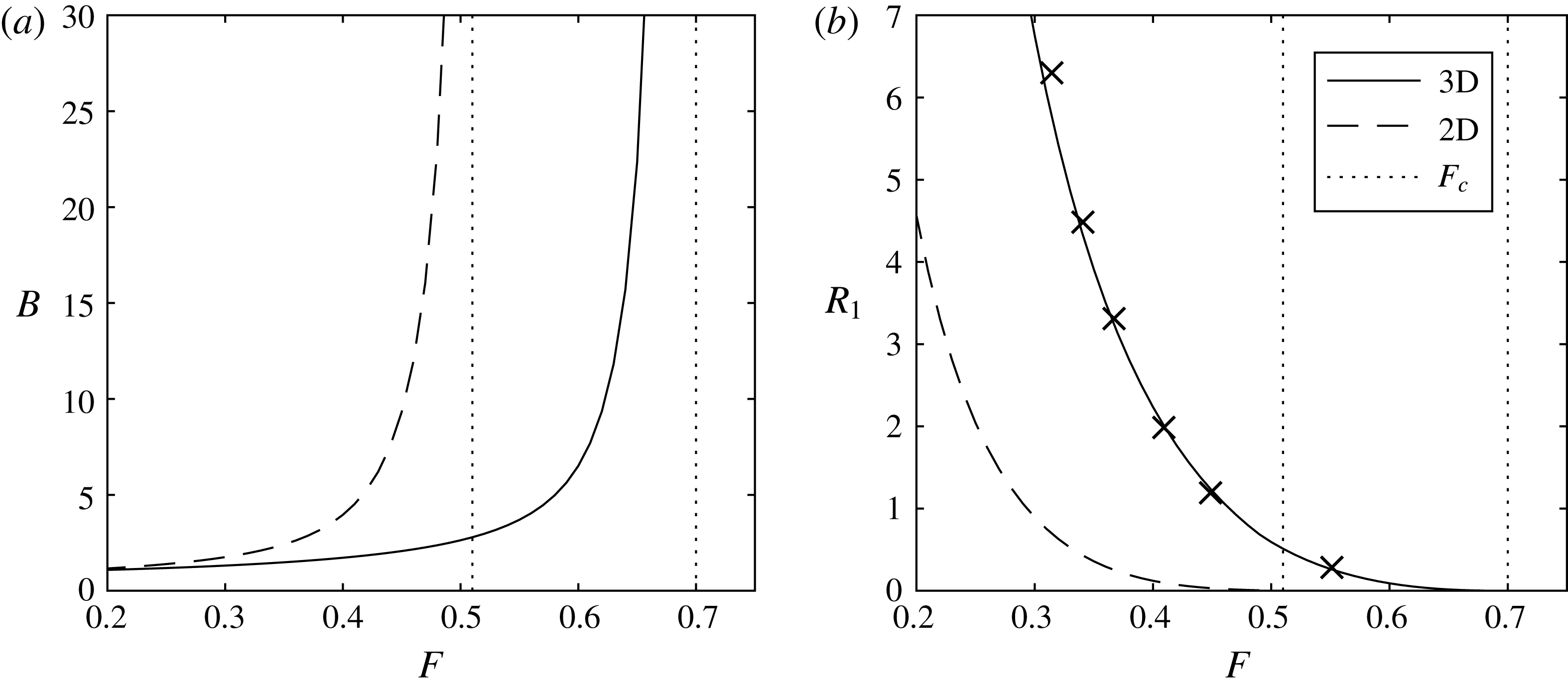
(a) Plot of the value of the constant
 $B$
given in (3.17) for the plane bubble and the constant
 $B$
in (3.9) for the axisymmetric bubble as a function of the Froude number
 $F$
for the zero surface tension case. As the solution branch approaches
 $F=F_{C}$
, the curvature at the apex becomes large and the value of
 $B\rightarrow \infty$
. This is shown in (b), where the radius of curvature of the streamline at the apex of the bubble,
 $R_{1}$
, goes to zero as
 $F\rightarrow F_{C}$
. The crosses show values obtained by Levine & Yang (Reference Levine and Yang1990).

The above method was used to compute solutions to both plane and axisymmetric bubbles with and without surface tension. Some profiles of axisymmetric
 $T=0$
solutions are shown in figure 3. As shown in figure 4, as we approach
 $F=F_{c}$
, the radius of curvature of the streamline becomes very small at the apex of the bubble (resulting in large values of the curvature). Since the
 $F=F_{c}$
solution is a pointed bubble with infinite curvature (computed in § 5), the constant
 $B$
associated with the corner singularity (3.9) is singular in the limit
 $F\rightarrow F_{c}$
. This made smooth bubbles with values of
 $F$
close to
 $F=F_{c}$
difficult to compute. We found that we required higher than double precision when computing these solutions in order for iterations in Newton’s method to convergence. This was done using MATLAB and the Advanpix (2017) multiprecision toolkit.
For the case of non-zero surface tension, we computed the first three solution branches
 $F_{1}(\unicode[STIX]{x1D6FC}),F_{2}(\unicode[STIX]{x1D6FC})$
and
 $F_{3}(\unicode[STIX]{x1D6FC})$
. When computing along solution branches, it is of significant importance that we are able to fix either
 $F$
or
 $\unicode[STIX]{x1D6FC}$
, and allow the other parameter to vary. In general, we found it more convenient to fix
 $\unicode[STIX]{x1D6FC}$
. Since there is now one additional unknown, we must introduce a new equation such that our discrete system is not ill posed. We impose a four-point interpolation formula on the curvature of the free surface, given by
 $$\begin{eqnarray}\displaystyle & \displaystyle K_{L,1}-3K_{L+1,1}+3K_{L+2,1}-K_{L+3,1}=0, & \displaystyle\end{eqnarray}$$
where
 $L>A+1$
is an integer such that
 $\unicode[STIX]{x1D719}_{L}>0$
. The motivation for using (4.1) is that, for a small range of values of
 $F$
around the solution branches
 $F_{i}(\unicode[STIX]{x1D6FC})$
, the method converges on unrealistic solutions with erratic curvature values. Alternatively, we occasionally fixed both
 $\unicode[STIX]{x1D6FC}$
and
 $F$
and manually moved through the solution space. This method was particularly useful when trying to obtain the first solution on a solution branch
 $F_{i}$
. Once on the solution branch, the code with varying
 $F$
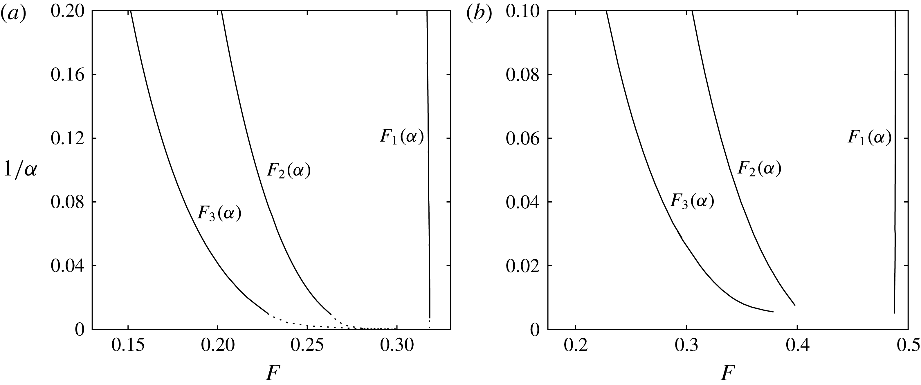
was used to compute solutions close to the one already obtained on the branch, using the previous solution as an initial guess. The first three solution branches for the plane and axisymmetric bubbles are shown in figure 5. The branch
 $F_{1}$
approaches
 $F^{\ast }$
. For higher-order branches, the numerical scheme fails to produce unique results for values of
 $\unicode[STIX]{x1D6FC}$
larger than shown in figure 5. Fixing both
 $\unicode[STIX]{x1D6FC}$
and
 $F$
, it is found the numerical scheme converges for all
 $F$
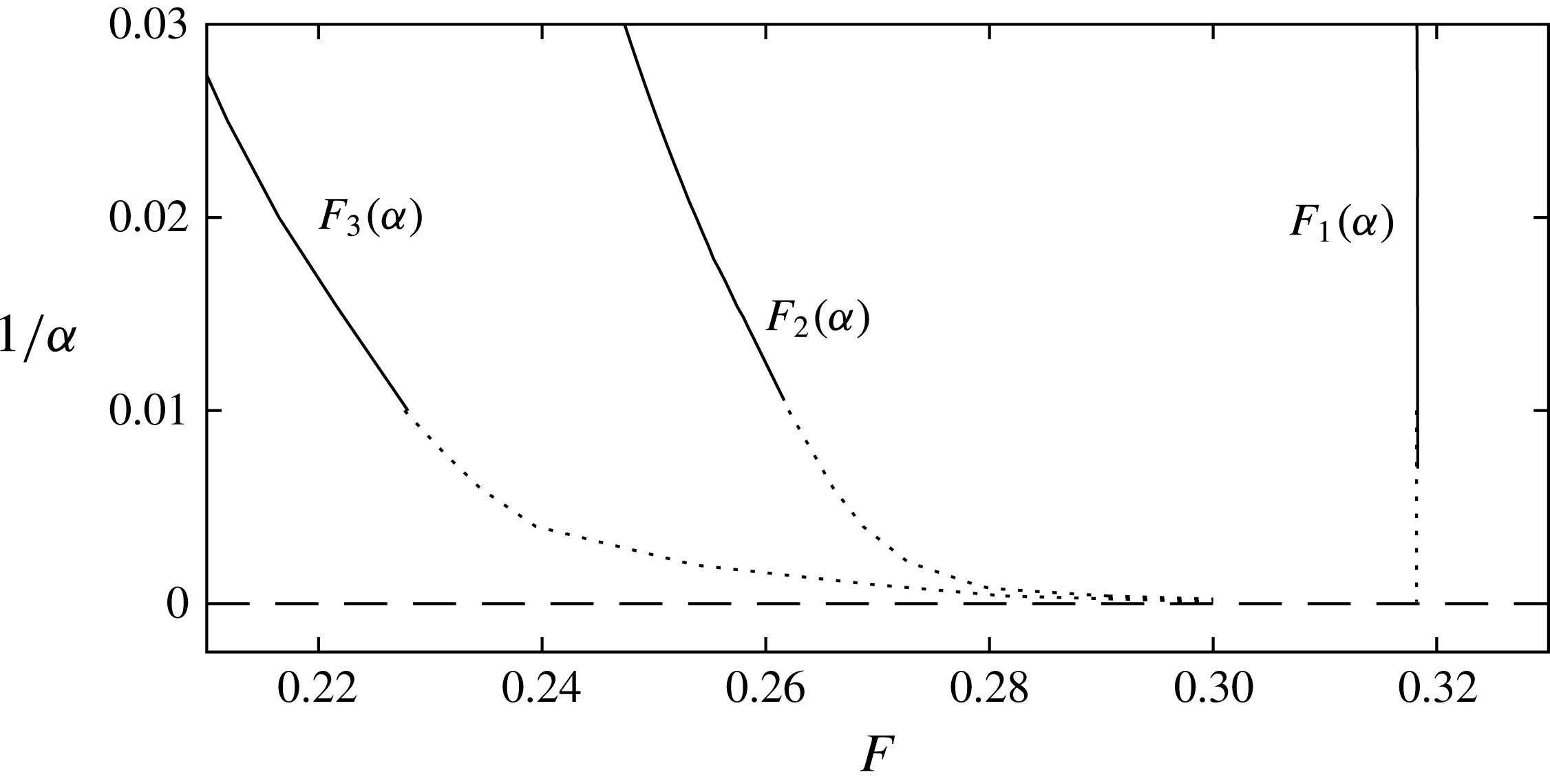
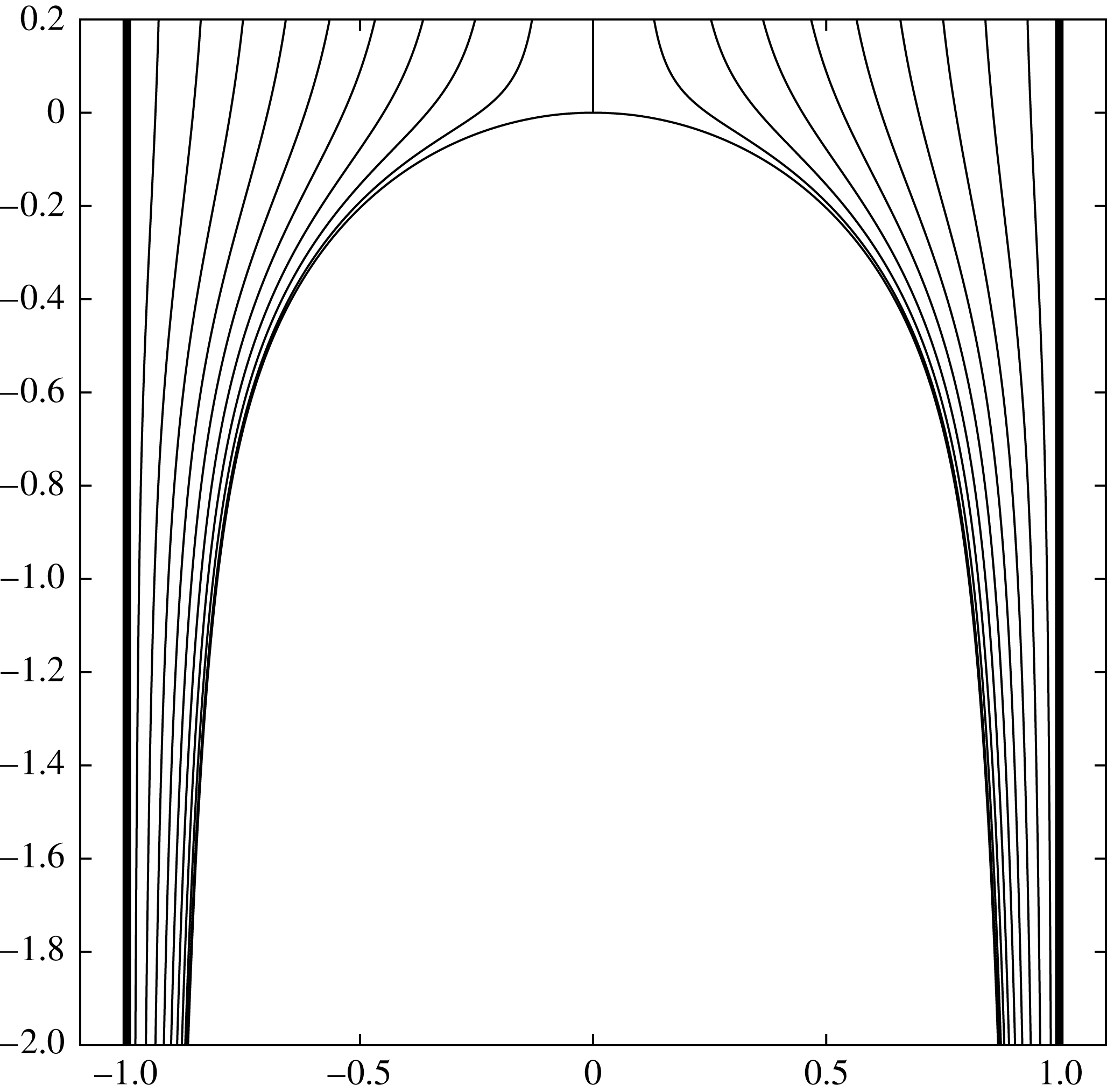
in this region. This is true for both the two-dimensional and axisymmetric problem. In figure 6, we show an enlarged plot of the limiting behaviour of the higher-order branches computed using the series truncation method for two-dimensional bubbles. Solutions computed using the series truncation method are very accurate, since, through the use of conformal mapping techniques, the numerical scheme is reduced to a one-dimensional problem (for a review of these methods, see Vanden-Broeck Reference Vanden-Broeck2010). This allows computations with thousands of mesh points on the free surface. As many as 10 000 points on the free surface were required to obtain solutions in this region of the solution space, far exceeding what is possible with our finite difference method. We conjecture that the higher-order branches of the axisymmetric bubbles have the same limiting behaviour, but a computationally less extensive numerical procedure would be required to compute solutions in this region. A plot of the selected axisymmetric solution
 $F^{\ast }$
is shown in figure 7.
The first three branches
 $F_{1}$
,
 $F_{2}$
and
 $F_{3}$
for the two-dimensional (a) and axisymmetric (b) bubbles. The dotted lines in (a) were computed using a series truncation method (see Vanden-Broeck Reference Vanden-Broeck1984b
).

A blow-up of figure 5(a), showing the limiting behaviour of the solution branches
 $F_{i}(\unicode[STIX]{x1D6FC})$
for the two-dimensional problem.

The selected axisymmetric solution
 $F^{\ast }=0.49$
, plotted to scale. Some streamlines are shown to demonstrate the flow field.

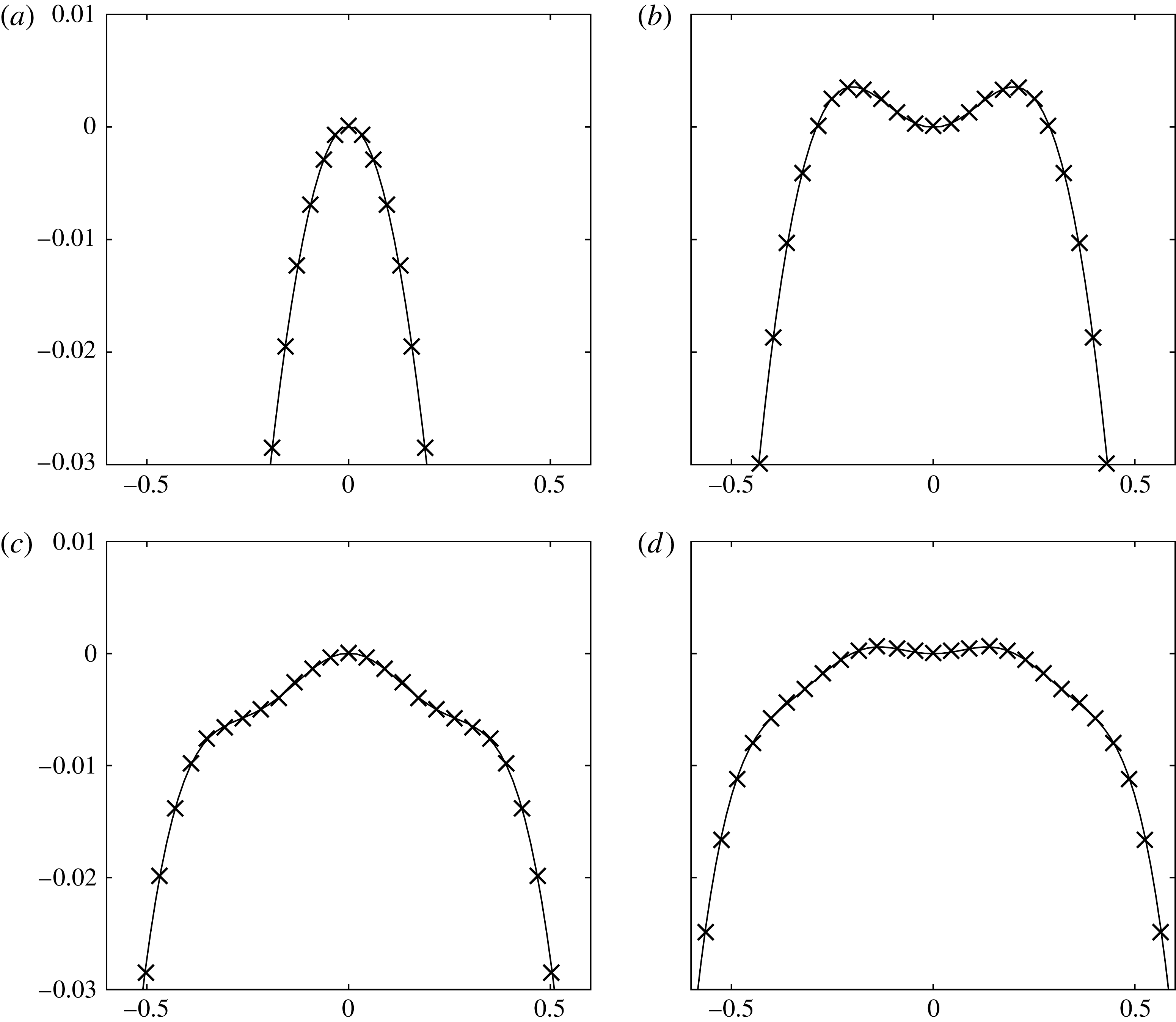
Profiles of smooth two-dimensional Taylor bubbles from the first four solution branches. The vertical scale has been exaggerated to show the oscillations clearly, and is the same for each figure. Every solution is given by
 $\unicode[STIX]{x1D6FC}=5$
, and the values of
 $F$
are (a)
 $F_{1}(5)=0.316$
, (b)
 $F_{2}(5)=0.202$
, (c)
 $F_{3}(5)=0.151$
and (d)
 $F_{4}(5)=0.122$
. The crosses are computed using a series truncation method (Vanden-Broeck Reference Vanden-Broeck1984a
), and agree with the results obtained using the finite difference scheme.

Profiles of axisymmetric Taylor bubbles from the first four solution branches. The vertical scale has been exaggerated to show the oscillations clearly, and is the same for each figure. Every solution is given by
 $\unicode[STIX]{x1D6FC}=10$
, and the values of
 $F$
are (a)
 $F_{1}(10)=0.488$
, (b)
 $F_{2}(10)=0.305$
, (c)
 $F_{3}(10)=0.228$
and (d)
 $F_{4}(10)=0.183$
.

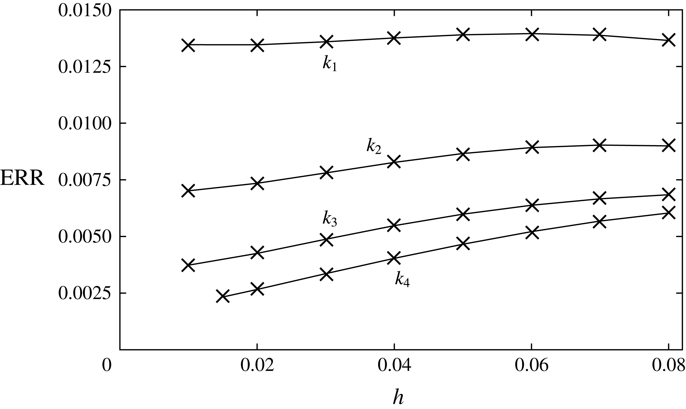
Plot of the relative errors in the value of
 $B$
for the
 $F=0.3$
two-dimensional bubble with zero surface tension for various mesh sizes. Denoting
 $B_{n}$
the value obtained by the numerical scheme, the relative error is defined as
 $\text{ERR}=|B_{e}-B_{n}|/B_{e}$
, where
 $B_{e}$
is the value obtained using the series truncation method. The curves are lines of constant
 $k$
, where the values of
 $k$
are
 $k_{1}=0.04$
,
 $k_{2}=0.02$
,
 $k_{3}=0.01$
and
 $k_{4}=0.005$
.

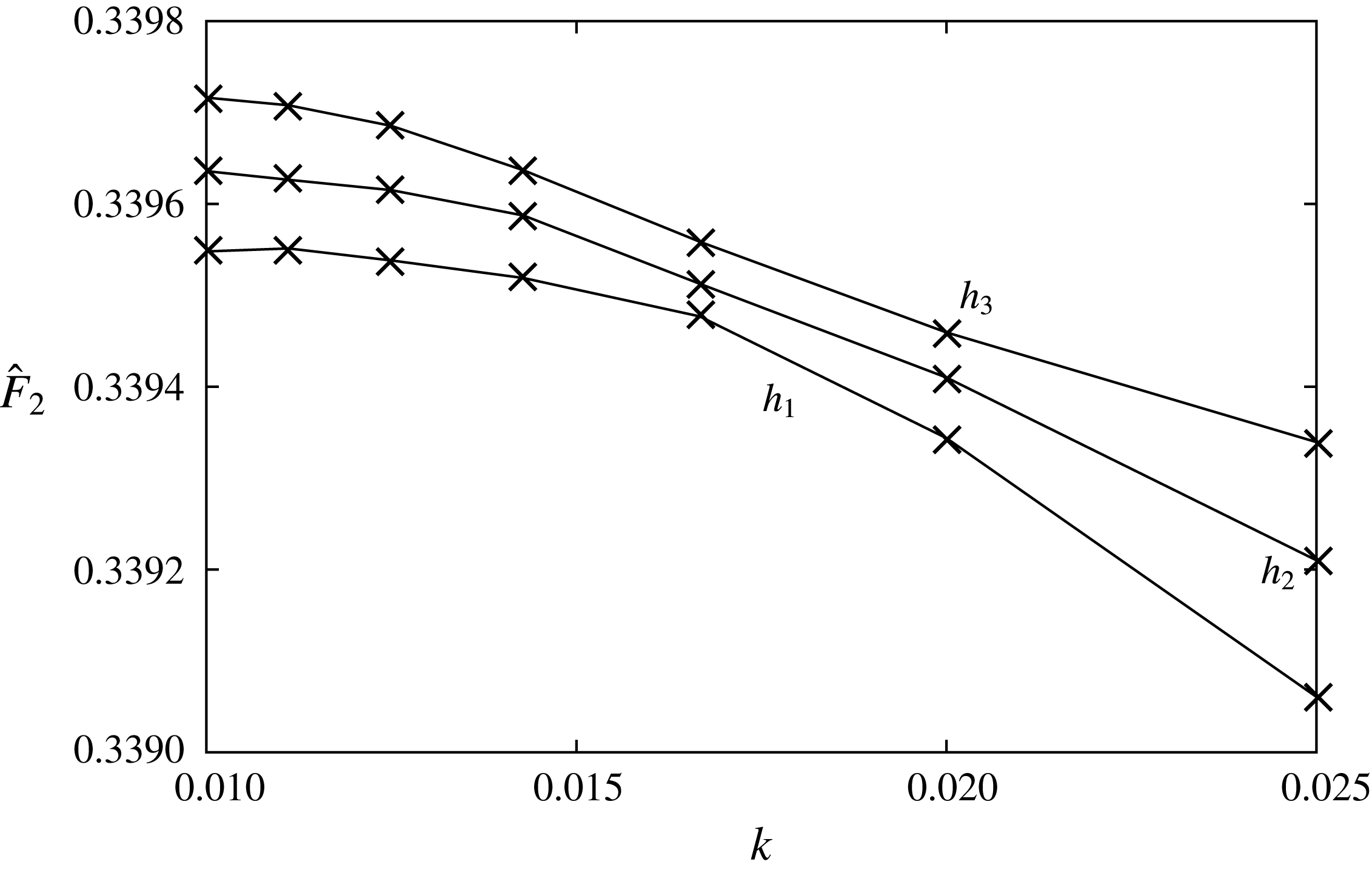
Values obtained for
 $F_{2}(20)=\hat{F}_{2}$
for the axisymmetric bubble. The curves are lines of constant
 $h$
, where the values of
 $h$
are
 $h_{1}=0.02$
,
 $h_{2}=0.01732$
and
 $h_{3}=0.015$
.

An interesting property of solutions on the higher mode solution branches is that they develop oscillations on the free surface. Figures 8 and 9 show solutions from the first four modes for a given
 $\unicode[STIX]{x1D6FC}$
for plane and axisymmetric bubbles respectively. Each odd mode
 $F_{2n-1}$
has a peak at the apex followed by
 $n-1$
peaks and troughs, while each even mode
 $F_{2n}$
has a trough at the apex, followed by
 $n$
peaks and
 $n-1$
troughs. Such behaviour was commented on by Levine & Yang (Reference Levine and Yang1990), who computed some higher mode solutions for larger values of the surface tension.
There are three main sources of error in the method: the approximation of derivatives via finite differences, the computation of
 $B$
in (3.11), and the truncation of the previously infinite flow domain
 $\unicode[STIX]{x1D6FA}_{\unicode[STIX]{x1D719}}$
. The error from domain truncation can be made negligible by taking
 $\unicode[STIX]{x1D719}_{1}$
and
 $\unicode[STIX]{x1D719}_{2}$
from (3.4) suitably large. For example, consider the axisymmetric bubble with zero surface tension and
 $F=0.34$
, computed with mesh spacing
 $h=0.02$
and
 $k=1/(60\sqrt{2})$
, where
 $h$
and
 $k$
are defined in (3.5). Comparing the solution obtained with
 $\unicode[STIX]{x1D719}_{1}\approx 4$
,
 $\unicode[STIX]{x1D719}_{2}\approx 20$
(denote
 $f=f_{1}(\unicode[STIX]{x1D719},\unicode[STIX]{x1D713})$
) and
 $\unicode[STIX]{x1D719}_{1}\approx 5$
,
 $\unicode[STIX]{x1D719}_{2}\approx 25$
(denote
 $f_{2}(\unicode[STIX]{x1D719},\unicode[STIX]{x1D713})$
), we find that
 $L^{\infty }|f_{1}-f_{2}|<10^{-13}$
.
In figure 10, we compare values of
 $B$
(see (3.17)) for the
 $T=0$
,
 $F=0.3$
two-dimensional bubble obtained using the series truncation with the value computed using the finite difference scheme for various
 $h$
and
 $k$
. Despite use of second-order finite differences, for fixed
 $k$
, the method appears to be slightly less than first-order convergent in
 $h$
. This is due to errors in approximating the constant
 $B$
in (3.11) at a mesh point close to the singularity. As
 $h$
is increased further, these inaccuracies grow and become
 $O(1)$
and larger, eventually leading to divergence of the Newton’s iterations. For fixed
 $h$
, the method is somewhere between first and second-order convergent in
 $k$
. The values of
 $h$
and
 $k$
for which we can obtain solutions are bounded below by computational memory (for example, taking
 $h=0.015,M=500$
and
 $N=101$
results in a
 $50\,500\times 50\,500$
Jacobian matrix). In figure 11, we compare values of
 $F_{2}(20)$
obtained for different values of
 $h$
and
 $k$
for the axisymmetric bubbles, demonstrating convergence of the numerical method. As an additional check on the numerical scheme, we note the good agreement between the profiles obtained by the series truncation method and the two-dimensional finite difference scheme in figure 8, and the results obtained by the boundary integral scheme of Levine & Yang (Reference Levine and Yang1990) for the axisymmetric bubbles, as seen in figure 4(b).
5 Pointed
 $F=F_{C}$
bubble

As described in the previous section, in the case of zero surface tension, as
 $F\rightarrow F_{C}$
, the curvature of the bubble at the apex becomes singular. The
 $F=F_{C}$
solution is a pointed bubble with interior angle
 $\unicode[STIX]{x1D707}=120$
for the two-dimensional problem, and
 $\unicode[STIX]{x1D707}\approx 115$
for the axisymmetric problem. In the following section, we compute the axisymmetric
 $F=F_{C}$
solution.
Garabedian (Reference Garabedian1985) derived a velocity potential describing the behaviour at the crest of the
 $F=F_{C}$
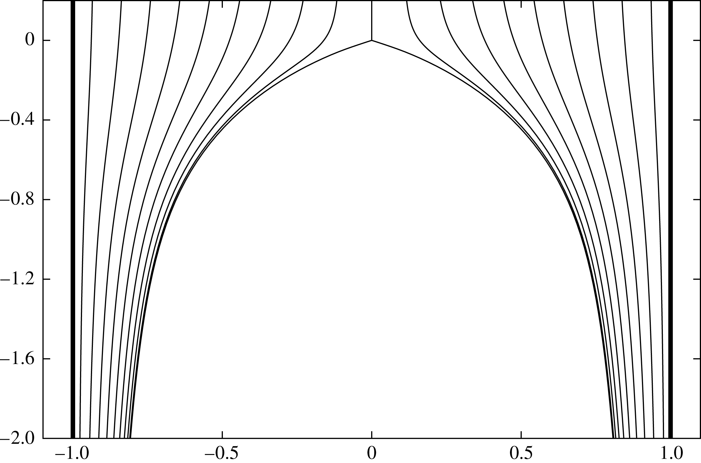
solution. The streamfunction can be found using relations (2.1), and is given by
 $$\begin{eqnarray}\displaystyle & \displaystyle \unicode[STIX]{x1D713}=Br^{2}(x^{2}+r^{2})^{1/4}\,\times \left\{\text{}_{2}F_{1}\left[-\frac{1}{2},\frac{7}{2},2,\frac{1}{2}\left(1+\frac{x}{(x^{2}+y^{2})^{1/2}}\right)\right]\right\}, & \displaystyle\end{eqnarray}$$
where
 $_{2}F_{1}$
is the Gaussian hypergeometric function, and
 $B$
is an arbitrary positive constant. A plot of some streamlines for
 $B=1$
is shown in figure 12.
Plots of streamlines given by (5.1)

Vanden-Broeck (Reference Vanden-Broeck1991) constructed a finite difference scheme with
 $r$
as an unknown function of the independent variables
 $(x,\unicode[STIX]{x1D713})$
. The flow domain in the
 $(x,\unicode[STIX]{x1D713})$
space is an infinite strip
 $\unicode[STIX]{x1D6FA}_{x}=\{\unicode[STIX]{x1D713}\in [0,1/2],-\infty <x<\infty \}$
, and can be discretised in a similar manner to
 $\unicode[STIX]{x1D6FA}_{\unicode[STIX]{x1D719}}$
in § 3. We again perform coordinate transforms (3.1a
, 3.1b
), replacing
 $\unicode[STIX]{x1D719}$
with
 $x$
in (3.1a
). We then discretise
 $\unicode[STIX]{x1D6FA}_{x}$
with
 $M$
points in
 $\unicode[STIX]{x1D6FC}$
and
 $N$
points in
 $t$
using (3.3). The governing equation, when formulated this way, is given by
 $$\begin{eqnarray}\displaystyle & \displaystyle r_{\unicode[STIX]{x1D713}\unicode[STIX]{x1D713}}\left(1+r_{x}^{2}\right)+r_{\unicode[STIX]{x1D713}}^{2}\left(r_{xx}+\frac{1}{r}\right)-2r_{x}r_{\unicode[STIX]{x1D713}}r_{x\unicode[STIX]{x1D713}}=0, & \displaystyle\end{eqnarray}$$
while Bernoulli’s equation yields
 $$\begin{eqnarray}\displaystyle & \displaystyle \left(1+r_{x}^{2}\right)\left(rr_{\unicode[STIX]{x1D713}}\right)^{-2}-\frac{2}{F^{2}}x=0. & \displaystyle\end{eqnarray}$$
Using these equations, we construct a discrete system of
 $MN$
equations similar to the system (3.6a
–3.6e
). Vanden-Broeck failed to account for the singularity in the flow field, resulting in divergence of the numerical method as the mesh is refined. We rectify this problem by making use of Garabedian’s solution (5.1). Like in § 3.1, we desire to find a solution
 $r(x,\unicode[STIX]{x1D713})=\unicode[STIX]{x1D712}(x,\unicode[STIX]{x1D713})$
which matches the singular behaviour of the bubble at the apex. Equation (5.1) is a transcendental equation for the unknown
 $r$
given a fixed point in the
 $(x,\unicode[STIX]{x1D713})$
space. This can be solved at each mesh point using Newton’s method to find
 $\unicode[STIX]{x1D712}$
. Equations for
 $\unicode[STIX]{x1D712}_{\unicode[STIX]{x1D713}}$
,
 $\unicode[STIX]{x1D712}_{x}$
,
 $\unicode[STIX]{x1D712}_{\unicode[STIX]{x1D713}\unicode[STIX]{x1D713}}$
,
 $\unicode[STIX]{x1D712}_{xx}$
and
 $\unicode[STIX]{x1D712}_{x\unicode[STIX]{x1D713}}$
can be obtained by differentiating (5.1) and making use of
 $$\begin{eqnarray}\displaystyle & \displaystyle r_{\unicode[STIX]{x1D713}}=\unicode[STIX]{x1D713}_{r}^{-1}, & \displaystyle\end{eqnarray}$$
 $$\begin{eqnarray}\displaystyle & \displaystyle r_{\unicode[STIX]{x1D713}\unicode[STIX]{x1D713}}=\unicode[STIX]{x1D713}_{r}^{-3}\unicode[STIX]{x1D713}_{rr}, & \displaystyle\end{eqnarray}$$
 $$\begin{eqnarray}\displaystyle & \displaystyle r_{x}=-\unicode[STIX]{x1D713}_{x}\unicode[STIX]{x1D713}_{r}^{-1}, & \displaystyle\end{eqnarray}$$
 $$\begin{eqnarray}\displaystyle & \displaystyle r_{x\unicode[STIX]{x1D713}}=\left(r_{x}r_{\unicode[STIX]{x1D713}\unicode[STIX]{x1D713}}-\unicode[STIX]{x1D713}_{rx}r_{\unicode[STIX]{x1D713}}^{3}\right)r_{\unicode[STIX]{x1D713}}^{-1}, & \displaystyle\end{eqnarray}$$
 $$\begin{eqnarray}\displaystyle & \displaystyle r_{xx}=\left(2r_{x}r_{\unicode[STIX]{x1D713}}r_{x\unicode[STIX]{x1D713}}-r_{x}^{2}r_{\unicode[STIX]{x1D713}\unicode[STIX]{x1D713}}-\unicode[STIX]{x1D713}_{xx}r_{\unicode[STIX]{x1D713}}^{3}\right)r_{\unicode[STIX]{x1D713}}^{-2}. & \displaystyle\end{eqnarray}$$
 $F_{C}\approx 0.7$
, in agreement with figure 5 and the results of Levine & Yang (Reference Levine and Yang1990). No solutions for other values of
 $F$
were found with this method, suggesting that
 $F=F_{C}$
is the only value of the Froude number for which zero surface tension axisymmetric bubbles are pointed with the singular behaviour (5.1) at the apex. It is known that two-dimensional Taylor bubbles with
 $F>F_{C}$
have cusps at the apex (see Vanden-Broeck Reference Vanden-Broeck1984a
). The authors were unable to obtain cusped axisymmetric bubbles since no suitable treatment of the cusp singularity was found.
Axisymmetric zero surface tension solution for
 $F=F_{C}\approx 0.70$
. Some streamlines are shown to demonstrate the flow field.

6 Conclusion
In conclusion, we have presented a numerical scheme capable of computing both two-dimensional and axisymmetric Taylor bubbles. The method used produces results in good agreement with previous authors. Two of the higher-order smooth solution branches,
 $F_{2}(\unicode[STIX]{x1D6FC})$
and
 $F_{3}(\unicode[STIX]{x1D6FC})$
, have been computed for small values of surface tension. Although unable to capture the limiting behaviour of the higher-order branches as
 $\unicode[STIX]{x1D6FC}\rightarrow \infty$
, similarities in the solution spaces of the two-dimensional and axisymmetric problems, combined with the knowledge of the limiting behaviour of the two-dimensional solution branches, provides numerical evidence to suggest the axisymmetric branches approach
 $F^{\ast }$
in the limit as
 $\unicode[STIX]{x1D6FC}\rightarrow \infty .$
We used the velocity potential derived by Garabedian (Reference Garabedian1985), combined with our singularity removal procedure, to compute the zero surface tension
 $F=F_{C}$
axisymmetric bubble, characterised by an interior angle of approximately
 $130^{0}$
. This was the only value of
 $F$
for which a pointed
 $T=0$
solution was found, further strengthening the similarities between the two-dimensional and axisymmetric solution spaces. The method presented in this paper could be used for a variety of axisymmetric flows, such as cavitating flow past an obstruction, flow leaving a vertical pipe onto an infinite plate (as considered in the two-dimensional case by Christodoulides & Dias Reference Christodoulides and Dias2010), or bubbles rising in unbounded mediums (see Yang & Levine Reference Yang and Levine1992).
Acknowledgements
A.D. was supported by EPSRC under grant EP/M507970/1. J.-M.V.-B. was supported in part by EPSRC under grant EP/N018559/1.