2. Transition analysis based on flow network

This study investigates hydrodynamic dispersion in statistically homogeneous porous media. The complex pore structure is simplified as a network of pores (nodes) connected by throats (tubes), a widely adopted approach in studies of flow and transport in porous media (Fatt Reference Fatt1956; Sahimi & Imdakm Reference Sahimi and Imdakm1988; Bijeljic, Muggeridge & Blunt Reference Bijeljic, Muggeridge and Blunt2004; Mehmani & Balhoff Reference Mehmani and Balhoff2015; Liu et al. Reference Liu, Gong, Zhao, Jin and Wang2022; Zhao et al. Reference Zhao, Qin, Kang, Qin, Derome and Carmeliet2022). In this model, pores are considered to have negligible volume, with solute fully mixed within each pore, and throats are simplified as straight tubes through which fluid flow follows the Poiseuille law.

The transport of solutes through the network is modelled within a CTRW framework (Dentz et al. Reference Dentz, Cortis, Scher and Berkowitz2004; Berkowitz et al. Reference Berkowitz, Cortis, Dentz and Scher2006), where solute transport is driven by the PDFs of transition length $\ell$ and transition time $\tau$ . We assume that $\ell$ and $\tau$ are independent random variables, with their respective PDFs denoted by $\omega (x)$ and $\psi (t)$ . This assumption is supported by the observed weak correlation in tracer velocities across different pores (Bijeljic, Mostaghimi & Blunt Reference Bijeljic, Mostaghimi and Blunt2011; de Anna et al. Reference de Anna, Le Borgne, Dentz, Tartakovsky, Bolster and Davy2013; Dentz et al. Reference Dentz, Kang, Comolli, Le Borgne and Lester2016; Alim et al. Reference Alim, Parsa, Weitz and Brenner2017). Within the framework, the longitudinal dispersion coefficient is derived as

(2.1) \begin{align} D_L &= \frac {\langle \ell \rangle ^2}{2 \langle \tau \rangle } \left ( \frac {\langle \tau ^2 \rangle - \langle \tau \rangle ^2}{\langle \tau \rangle ^2} + \frac {\langle \ell ^2 \rangle - \langle \ell \rangle ^2}{\langle \ell \rangle ^2} \right ). \end{align}

A detailed derivation of this expression is provided in the supplementary material is available at https: https://doi.org/10.1017/jfm.2025.11049, see also Dentz et al. (Reference Dentz, Cortis, Scher and Berkowitz2004). Here, the moments are defined as

(2.2) \begin{align} \langle \tau \rangle &= \int t \, \psi (t) \, {\textrm d}t, \quad \langle \tau ^2 \rangle = \int t^2 \, \psi (t) \, {\textrm d}t, \end{align}

(2.3) \begin{align} \langle \ell \rangle &= \int x \, \omega (x) \, {\textrm d}x, \quad \langle \ell ^2 \rangle = \int x^2 \, \omega (x) \, {\textrm d}x. \end{align}

Since the PDF $\psi (t)$ generally exhibits a much broader distribution than the PDF $\omega (x)$ in porous media, this implies that $ {\langle \tau ^2 \rangle - \langle \tau \rangle ^2}/{\langle \tau \rangle ^2} \gg {\langle \ell ^2 \rangle - \langle \ell \rangle ^2}/{\langle \ell \rangle ^2}$ , the longitudinal dispersion coefficient scales approximately as

(2.4) \begin{align} D_L &\sim \frac {\langle \ell \rangle ^2}{\langle \tau \rangle } \frac {\langle \tau ^2 \rangle - \langle \tau \rangle ^2}{\langle \tau \rangle ^2}. \end{align}

It should be noted that (2.1)–(2.4) are valid only when the second-order moments, $\langle \tau ^2 \rangle$ and $\langle \ell ^2 \rangle$ , exist and remain finite. This condition is always satisfied in the cases considered here. Specifically, for statistically homogeneous porous media, the finite tube lengths ensure that $\langle \ell ^2 \rangle$ remains finite, while molecular diffusion imposes an upper bound on the transition time, guaranteeing that $\langle \tau ^2 \rangle$ is also finite.

Equation (2.4) indicates the essential role of the global PDF of transition times, $\psi (t)$ , in the scaling relationship between the dispersion coefficient, $D_L$ , and the Péclet number, ${\textit{Pe}}$ . The PDF $\psi (t)$ is shaped by both intra-pore and inter-pore flow variabilities (Liu et al. Reference Liu, Xiao, Aquino, Dentz and Wang2024c ), which are characterised by $\psi _t(t|\zeta )$ , the local PDF of tracer transition time through an individual conduit, and $\hat {\psi }_\zeta (t)$ , the PDF of minimal advection times $\zeta$ associated with the tubes that tracers choose to enter at pore junctions, respectively. The minimal advection time $\zeta$ is defined as $\zeta = l / v$ , where $v$ represents the maximal velocity within the tube.

The local PDF $\psi _t(t|\zeta )$ depends on the minimal advection time $\zeta$ through the tube and can be categorised into three distinct modes. Mode I corresponds to $\zeta \lt \zeta _{\text{D,R}}$ , where radial and axial diffusion are negligible. Tracers move along streamlines with their transition times through the tube determined by advection. Mode II arises when $\zeta _{\text{D,R}} \leqslant \zeta \lt \zeta _{D,l}$ . The tracers are fully mixed across the transverse direction, and the transition time distribution is strongly peaked near the mean advection time $2\zeta$ . Mode III occurs when $\zeta \geqslant \zeta _{D,l}$ , indicating that advection is slower than molecular diffusion; under this condition, the transition times converge to approximately $\zeta _{D,l}$ . Although backward tracer motion can occur near tube entrances (Aquino & Dentz Reference Aquino and Dentz2018), its influence on hydrodynamic dispersion is minimal and is therefore neglected in this study. Liu et al. (Reference Liu, Xiao, Aquino, Dentz and Wang2024c ) derive the local PDF $\psi _t(t|\zeta )$ as

(2.5) \begin{align} \psi _t(t|\zeta ) = \begin{cases} 2 \zeta ^2 t^{-3} H(t - \zeta ) H(\zeta _B - t), & (\zeta \lt \zeta _{D,R}), \\ \delta (t - 2\zeta ), & (\zeta _{D,R} \leqslant \zeta \lt \zeta _{D,l}), \\ \delta (t - \zeta _{D,l}), & (\zeta \geqslant \zeta _{D,l}), \end{cases} \end{align}

where $H$ is the Heaviside step function, and $\zeta _{D,R}$ and $\zeta _{D,l}$ represent the radial and axial diffusion times, respectively. The diffusion times are calculated as $\zeta _{D,R} = {R^2}/{D_m}$ and $\zeta _{D,l} = {l^2}/{D_m}$ , where $R$ and $l$ represent the radius and the length of the tube, and $D_m$ denotes the molecular diffusion coefficient. Additionally, $\zeta _B$ denotes the truncation time and is given by

(2.6) \begin{align} \zeta _B = \zeta \sqrt {\frac {vR^2}{8 D_m l}}. \end{align}

The PDF $\hat {\psi }_\zeta (t)$ is determined as the flux-weighted PDF of advection times

(2.7) \begin{align} \hat {\psi }_\zeta (t) = \frac {1}{\sum _{{i}=1}^{N_0} q_{{i}}} \sum _{{i}=1}^{N_0} q_{{i}} \delta (t - \zeta _{{i}}), \end{align}

where $N_0$ represents the total number of tubes, $q$ denotes the flow rate through a tube and the subscript $i$ indexes each tube.

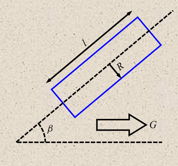
The PDF $\hat {\psi }_\zeta (t)$ is governed by the inter-pore flow variability, which originates from the random distribution of tube properties within the network, as illustrated in figure 1. These properties include the tube radius $R$ , length $l$ and orientation angle $\beta$ . According to the Poiseuille law, the hydraulic conductance $g$ of a pore throat – defined as the volumetric flow rate per unit pressure drop – scales as $g \sim R^{4} l^{-1}$ . Under the assumption of a uniform macroscopic pressure gradient $G = |\boldsymbol{\nabla }p|$ along the mean flow direction, which is reasonable for statistically homogeneous porous media (Scheidegger Reference Scheidegger1954), the pressure drop across an individual pore throat is given by $\Delta p = G l \cos \beta$ . Consequently, the following scaling relationships are obtained:

(2.8) \begin{align} q &\sim R^{4} G \cos \beta , \end{align}

(2.9) \begin{align} v &\sim R^{2} G \cos \beta , \end{align}

(2.10) \begin{align} \zeta &\sim l R^{-2} G^{-1} \cos ^{-1} \beta . \end{align}

By substituting (2.8) and (2.10) into (2.7), the PDF $\hat {\psi }_\zeta (t)$ can be expressed as a function of the randomly distributed geometric properties of tubes within the network

(2.11) \begin{align} \hat {\psi }_\zeta (t) = \frac {1}{\sum _{{i}=1}^{N_0} R_{i}^{4} \cos \beta _{i}} \sum _{{i}=1}^{N_0} R_{i}^{4} \cos \beta _{i} \delta \big(t - \varTheta l_{i} R_{i}^{-2} G^{-1} \cos ^{-1} \beta _{i}\big), \end{align}

where $\varTheta = \zeta / (l R^{-2} G^{-1} \cos ^{-1} \beta )$ is a coefficient associated with the tube cross-sectional shape. Assuming all tubes possess circular cross-sections, this coefficient simplifies to $\varTheta = 4\mu$ , with $\mu$ denoting the fluid viscosity. Consequently, the PDF $\hat {\psi }_\zeta (t)$ is completely determined from the statistical distributions of the tube radius $R$ , length $l$ and orientation angle $\beta$ , which can be obtained through structural characterisation such as computed tomography (CT) imaging.

Figure 1.

Schematic illustration of a single tube (blue rectangle) within the tube network. Here, $R$ represents the tube radius, $l$ the tube length, $G$ the mean pressure gradient directed from left to right and $\beta$ the angle between the tube axis and the mean flow direction.

The minimum and maximum advection times within the network are represented by $\zeta _{\textit{min}}$ and $\zeta _{\textit{max}}$ , respectively. When the ratio $\zeta _{\textit{max}} / \zeta _{\textit{min}}$ is large, the PDF $\hat {\psi }_\zeta (t)$ can be effectively modelled as a power-law function (de Anna et al. Reference de Anna, Quaife, Biros and Juanes2017; Dentz, Icardi & Hidalgo Reference Dentz, Icardi and Hidalgo2018; Liu et al. Reference Liu, Xiao, Aquino, Dentz and Wang2024c ),

(2.12) \begin{align} \hat {\psi }_\zeta (t) \sim t^{-2-\theta }, \quad t \in [\zeta _{\textit{min}}, \zeta _{\textit{max}}]. \end{align}

Here, $\theta$ is constrained to be positive to ensure an asymptotic regime of dispersion. In contrast, when the ratio $\zeta _{\textit{max}} / \zeta _{\textit{min}}$ is small, the PDF $\hat {\psi }_\zeta (t)$ is approximated by a Dirac-delta function (Liu et al. Reference Liu, Xiao, Aquino, Dentz and Wang2024c )

(2.13) \begin{align} \hat {\psi }_\zeta (t) \sim \delta (t - \zeta _{\textit{min}}). \end{align}

The global PDF $\psi (t)$ is given by the marginalisation of the joint PDF $\psi _t(t|t') \hat {\psi }_\zeta (t')$

(2.14) \begin{align} \psi (t) = \int _{\zeta _{\textit{min}}}^{\zeta _{\textit{max}}} \psi _t(t|t') \hat {\psi }_\zeta (t') \, {\textrm d}t'. \end{align}

The nature of $\psi (t)$ is shaped by the interplay between $\psi _t(t|\zeta )$ and $\hat {\psi }_\zeta (t)$ , which represent intra-pore and inter-pore flow variability, respectively. Specifically, when $\hat {\psi }_\zeta (t)$ exhibits slower decay and a broader distribution than $\psi _t(t|\zeta )$ , that is, when $0 \lt \theta \lt 1$ and $\zeta _{\textit{max}} / \zeta _{\textit{min}} \gt 100$ (Liu et al. Reference Liu, Xiao, Aquino, Dentz and Wang2024c ), the PDF $\psi (t)$ is primarily determined by $\hat {\psi }_\zeta (t)$ . In contrast, when these conditions are not satisfied, the PDF $\psi (t)$ is predominantly influenced by the PDF $\psi _t(t|\zeta )$ .

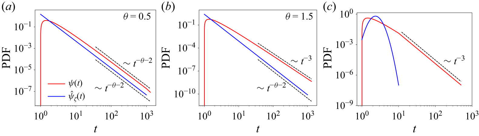
Under the conditions $0 \lt \theta \lt 1$ and $\zeta _{\textit{max}} / \zeta _{\textit{min}} \gt 100$ , as demonstrated in figure 2( $a$ ), the global PDF $\psi (t)$ follows the relation (Liu et al. Reference Liu, Xiao, Aquino, Dentz and Wang2024c )

(2.15) \begin{align} \psi (t) \sim t^{-\theta - 2}. \end{align}

At intermediate Péclet numbers ${\textit{Pe}}$ , the transition times are constrained between $\zeta _{\textit{min}}$ and $\zeta _{D,l}$ . The first and second moments of the transition times scale as

(2.16) \begin{align} \langle \tau \rangle \sim \textit{Pe}^{-1}, \quad \langle \tau ^2 \rangle \sim \textit{Pe}^{-\theta - 1}. \end{align}

By substituting (2.16) into (2.4), the dispersion coefficient exhibits a superlinear scaling relationship as

(2.17) \begin{align} \frac {D_L}{D_m} \sim {Pe}^{-\theta + 2}. \end{align}

Figure 2.

Comparison of the global PDF $\psi (t)$ for transition times with the flux-weighted PDF $\hat {\psi }_\zeta (t)$ for advection times in porous media with varying levels of inter-pore flow variability: ( $a$ ) $\zeta _{\textit{max}} / \zeta _{\textit{min}} = 1000$ and $\theta = 0.5$ , ( $b$ ) $\zeta _{\textit{max}} / \zeta _{\textit{min}} = 1000$ and $\theta = 1.5$ and ( $c$ ) small ratio of $\zeta _{\textit{max}} / \zeta _{\textit{min}}$ . In panel ( $a$ ), the global PDF $\psi (t)$ is primarily influenced by inter-pore flow variability, characterised by the PDF $\hat {\psi }_\zeta (t)$ . In contrast, panels ( $b$ ) and ( $c$ ) illustrate scenarios where the global PDF $\psi (t)$ is predominantly affected by intra-pore flow variability, represented by the PDF $\psi _t(t|\zeta ) \sim t^{-3}$ .

In contrast, when $\theta \gt 1$ or $\zeta _{\textit{max}} / \zeta _{\textit{min}} \lt 100$ , the global PDF $\psi (t)$ is derived as (Liu et al. Reference Liu, Xiao, Aquino, Dentz and Wang2024c )

(2.18) \begin{align} \psi (t) \sim t^{-3}. \end{align}

This behaviour is illustrated in figures 2( $b$ ) and 2( $c$ ). Under these conditions, the first and second moments of the transition times scale as

(2.19) \begin{align} \langle \tau \rangle \sim {Pe}^{-1}, \quad \langle \tau ^2 \rangle \sim {Pe}^{-2} \ln ({Pe}). \end{align}

Consequently, the superlinear scaling relationship changes to

(2.20) \begin{align} \frac {D_L}{D_m} \sim {Pe} \ln ({Pe}). \end{align}

This logarithmic superlinear scaling is consistent with the results presented by Saffman (Reference Saffman1959).

The variability of inter-pore flow is quantified using the coefficient of variation, defined as

(2.21) \begin{align} CV = \frac {\sqrt {\langle \zeta ^2 \rangle - \langle \zeta \rangle ^2}}{\langle \zeta \rangle }, \end{align}

where

(2.22) \begin{align} \langle \zeta \rangle = \int _{\zeta _{\textit{min}}}^{\zeta _{\textit{max}}} t \hat {\psi }_\zeta (t) \, {\textrm d}t, \quad \langle \zeta ^2 \rangle = \int _{\zeta _{\textit{min}}}^{\zeta _{\textit{max}}} t^2 \hat {\psi }_\zeta (t) \, {\textrm d}t. \end{align}

A larger value of $CV$ indicates increased variability in inter-pore flow.

For cases where $\theta \neq 1$ , $CV$ is expressed as a function of $\theta$ and the ratio $\zeta _{\textit{max}}/\zeta _{\textit{min}}$

(2.23) \begin{align} CV = \sqrt {\frac {\theta ^2}{\theta ^2 - 1} \frac {\left (1 - \left (\zeta _{\textit{max}} / \zeta _{\textit{min}} \right )^{\theta - 1}\right ) \left (1 - \left (\zeta _{\textit{max}} / \zeta _{\textit{min}} \right )^{\theta + 1}\right )}{\left (1 - \left (\zeta _{\textit{max}} / \zeta _{\textit{min}} \right )^\theta \right )^2} - 1}. \end{align}

For the case where $\theta = 1$ , $CV$ is expressed as

(2.24) \begin{align} CV = \sqrt {\frac {1}{2} \ln \left (\zeta _{\textit{max}} / \zeta _{\textit{min}}\right ) - 1}. \end{align}

The value of $CV$ increases with the ratio of $\zeta _{\textit{max}} / \zeta _{\textit{min}}$ but decreases with increasing $\theta$ , as illustrated in figure 3( $a$ ). This trend indicates that, when $0 \lt \theta \lt 1$ and $\zeta _{\textit{max}} / \zeta _{\textit{min}} \gt 100$ , the value of $CV$ must exceed a critical threshold $CV_c$ , which is defined as

(2.25) \begin{align} CV_c = max \{CV_{\theta =1,\zeta _{\textit{max}} / \zeta _{\textit{min}}}, CV_{\theta ,\zeta _{\textit{max}} / \zeta _{\textit{min}} = 100}\}. \end{align}

As shown by the dashed lines in figure 3( $a$ ), the variation of $CV$ becomes negligible when $\theta =1$ or $\zeta _{\textit{max}} / \zeta _{\textit{min}}=100$ . Hence, $CV_c$ can be reasonably approximated as

(2.26) \begin{equation} \begin{aligned} CV_c &\approx CV_{\theta =1,\zeta _{\textit{max}} / \zeta _{\textit{min}} = 100} \\ &\approx 1.14. \end{aligned} \end{equation}

Figure 3.

( $a$ ) Coefficient of variation for advection times ( $CV$ ) in networks with varying $\zeta _{\textit{max}}/\zeta _{\textit{min}}$ ratios and $\theta$ values. ( $b$ ) Contour plot of $\chi$ values as a function of the $\zeta _{\textit{max}}/\zeta _{\textit{min}}$ ratio and $\theta$ value, and ( $c$ ) the corresponding two-dimensional projection. For $\chi \gt 1$ , the superlinear scaling relationship is predominantly influenced by inter-pore flow variability, whereas for $\chi \lt 1$ , intra-pore flow variability becomes the dominant factor. ‘Intra-FV’ and ‘Inter-FV’ are abbreviations for intra-pore flow variability and inter-pore flow variability, respectively.

Although (2.23) and (2.24) define $CV$ in terms of $\theta$ and the ratio $\zeta _{\textit{max}}/\zeta _{\textit{min}}$ , these parameters are derived a posteriori. In the following, we explicitly derive $CV$ as a function of the randomly distributed geometric characteristics of the tubes within the network. By substituting (2.11) into (2.22), the first and second moments of $\zeta$ , namely $\langle \zeta \rangle$ and $\langle \zeta ^2 \rangle$ , are obtained as follows:

(2.27) \begin{align} \langle \zeta \rangle & = \frac {\varTheta G^{-1}}{\sum _{{i}=1}^{N_0} R_{i}^{4} \cos \beta _{i}} \sum _{{i}=1}^{N_0} R_{i}^{2} l_{i}, \end{align}

(2.28) \begin{align} \langle \zeta ^2 \rangle & = \frac {\varTheta ^2 G^{-2}}{\sum _{{i}=1}^{N_0} R_{i}^{4} \cos \beta _{i}} \sum _{{i}=1}^{N_0} l_{i}^{2} \cos ^{-1} \beta _{i}. \end{align}

Finally, substituting (2.27) and (2.28) into (2.21) yields an explicit expression for $CV$ in terms of the geometrical properties of the network

(2.29) \begin{align} CV = \sqrt {\frac {\frac {1}{\sum _{{i}=1}^{N_0} R_{i}^{4} \cos \beta _{i}} \sum _{{i}=1}^{N_0} l_{i}^{2} \cos ^{-1} \beta _{i}}{\left(\frac {1}{\sum _{{i}=1}^{N_0} R_{i}^{4} \cos \beta _{i}} \sum _{{i}=1}^{N_0} R_{i}^{2} l_{i}\right)^2} - 1}. \end{align}

Our previous work (Liu et al. Reference Liu, Xiao, Aquino, Dentz and Wang2024c ) has already demonstrated that the superlinear scaling behaviour of hydrodynamic dispersion in porous media can be divided into two distinct regimes: one governed by inter-pore flow variability and the other by intra-pore flow variability. This classification, however, was based on the nature of the PDF $\hat {\psi }_\zeta (t)$ , characterised by the parameters $\theta$ and $\zeta _{\textit{max}} / \zeta _{\textit{min}}$ . These parameters are a posteriori quantities that cannot be directly obtained from measurable properties. To overcome this limitation, the present study introduces a new dimensionless parameter, $\chi$ , defined as

(2.30) \begin{align} \chi = \frac {CV}{CV_c}, \end{align}

where $CV_c$ and $CV$ are given by (2.26) and (2.29), respectively. A value of $\chi \gt 1$ – which corresponds to $0 \lt \theta \lt 1$ and $\zeta _{\textit{max}} / \zeta _{\textit{min}} \gt 100$ – indicates that inter-pore flow variability predominantly contributes to the observed superlinear scaling behaviour. In contrast, $0 \lt \chi \lt 1$ signifies that intra-pore flow variability becomes the controlling factor, as shown in figures 3( $b$ ) and 3( $c$ ). Importantly, the value of $\chi$ is derived exclusively from the statistical distributions of the tube radius ( $R$ ), length ( $l$ ) and orientation angle ( $\beta$ ) within the network, which can be obtained through structural characterisation techniques such as CT imaging.

3. Numerical methods

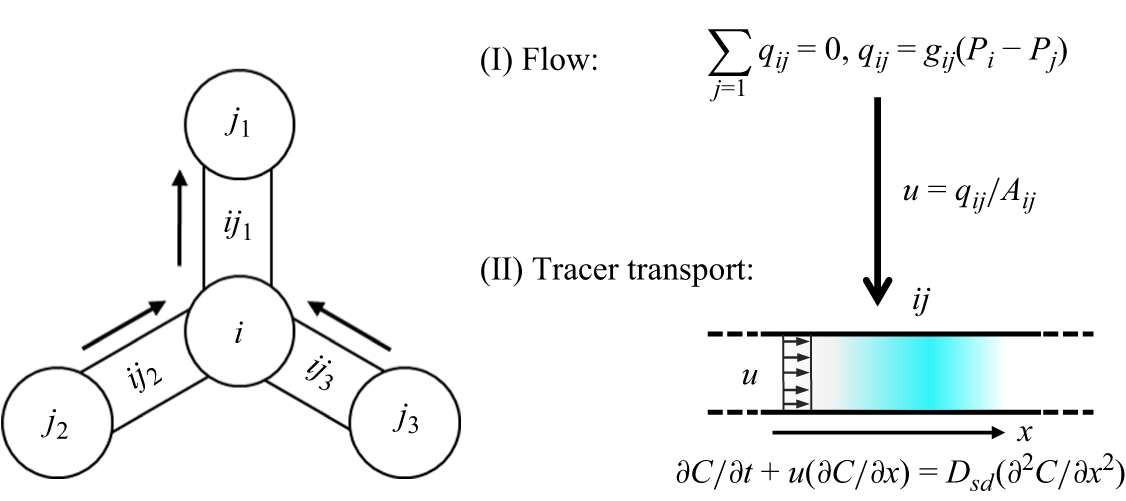
This section presents the network model employed to simulate fluid flow and solute transport in porous media. A comprehensive description of this model was provided in our previous work (Liu et al. Reference Liu, Gong, Zhao, Jin and Wang2022, Reference Liu, Gong, Xiao and Wang2024b ); here, we present a concise overview. In this model, the pore structure is simplified as a network of pores interconnected by throats. A schematic of the numerical framework is shown in figure 4. The simulation procedure starts by determining the flow field, followed by the simulation of solute transport, both governed by mass conservation at each node.

Figure 4.

Schematic of flow and tracer transport between pores in the network model.

3.1. Network model for fluid flow

In the network model, fluid flow through porous media is analogous to electrical current flowing through a resistor network. The flow field is determined by solving a set of linear equations constructed from local hydraulic conductance and the specified boundary conditions. The hydraulic conductance for a single tube is calculated as

(3.1) \begin{align} g = \frac {\epsilon A^2}{\mu l}, \end{align}

where $A$ is the cross-sectional area, $l$ is the conduit length and $\mu$ denotes the fluid viscosity. The coefficient $\epsilon$ depends on the cross-sectional shape. In this study, we consider only tubes with circular cross-sections, for which $\epsilon = 1/(8\pi )$ .

The flow rate $q_{\textit{ij}}$ between two connected pores, $i$ and $j$ , is expressed as

(3.2) \begin{align} q_{\textit{ij}} = g_{\textit{ij}} (P_i - P_j), \end{align}

where $P_i$ and $P_j$ stand for the pressure in pore $i$ and pore $j$ , respectively, and $g_{\textit{ij}}$ is the hydraulic conductance of the tube connecting these two pores. Given the pressure drop between the inlet and outlet of the network, the pressure in each pore is determined by applying the mass conservation law at every pore. For example, considering pore $i$ ,

(3.3) \begin{align} \sum _j q_{\textit{ij}} = 0. \end{align}

Once the pore pressures are determined, they are substituted into (3.2) to calculate the flow rate $q_{\textit{ij}}$ for each tube. Subsequently, the mean velocity within each tube is calculated as

(3.4) \begin{align} u = \frac {q_{\textit{ij}}}{A}. \end{align}

3.2. Network model for solute transport

The transport of solute through the network is modelled using a mixed-cell network model, in which solute is assumed to be fully mixed within each pore. Solute transport occurs through both advection and diffusion, with the evolution of the concentration governed by mass conservation at each pore and throat. For the control volume of pore $i$ , the mass conservation is described by

(3.5) \begin{equation} V_i \frac {\textrm{d}{\kern0.5pt}C_i}{\textrm{d}{\kern0.5pt}t} = \sum _{j \in {in}} q_{\textit{ij}} \boldsymbol{\cdot }C_{\textit{ij}} - \sum _{j \in {out}} q_{\textit{ij}} \boldsymbol{\cdot }C_i + \sum _j \left ( \dfrac {C_{\textit{ij}} - C_i}{\dfrac {l_i}{D_{\textit{sd},i} A_i} + \dfrac {0.5 l_{\textit{ij}}}{D_{\textit{sd},ij} A_{\textit{ij}}}} \right ). \end{equation}

The term on the left-hand side of the equation represents the net mass accumulation within the control volume, while the terms on the right-hand side account for mass exchange due to advective inflow, advective outflow and diffusive mass exchange, respectively. Here, $C$ and $V$ refer to the concentration and the volume, respectively. The corresponding quantities for throat $ij$ and pore $i$ are denoted with the subscript $ij$ and $i$ , respectively. The term $D_{\textit{sd}}$ denotes the pore-scale shear dispersion coefficient, which reproduces the effect of parabolic velocity profiles on mass transfer within individual pores or throats. The value of $D_{\textit{sd}}$ is calculated as

(3.6) \begin{equation} \frac {D_{\textit{sd}}}{D_m} - 1 = {\frac {1}{192} \left(\frac {vR}{D_m}\right)^2} \left [ 1 - \exp \left ( -2\alpha \frac {D_m \zeta }{R^2} \right ) \right ], \end{equation}

where $\alpha$ is a coefficient dependent on the shape of the conduit cross-sections, with values of 15, 10.8 and 4.8 for conduits with circular, square and triangular cross-sections, respectively. For the control volume of throat $ij$ , the mass conservation is expressed as

(3.7) \begin{equation} V_{\textit{ij}} \frac {{\textrm d}C_{\textit{ij}}}{{\textrm d}t} = q_{\textit{ij}} (C_{\textit{in}} - C_{\textit{out}}) + \frac {C_i - C_{\textit{ij}}}{\frac {l_i}{D_{\textit{sd},i} A_i} + \frac {0.5 l_{\textit{ij}}}{D_{\textit{sd},ij} A_{\textit{ij}}}} + \frac {C_j - C_{\textit{ij}}}{\frac {l_j}{D_{\textit{sd},j} A_j} + \frac {0.5 l_{\textit{ij}}}{D_{\textit{sd},ij} A_{\textit{ij}}}}, \end{equation}

where $C_{\textit{in}}$ and $C_{\textit{out}}$ are the inflow and outflow concentrations, respectively. An implicit scheme is employed to solve the concentration field.

The reliability and accuracy of our network algorithm have been validated through rigorous comparisons with direct numerical simulations solutions and experimental data, demonstrating relative errors of less than $6 \,\%$ in predicted permeability (Liu et al. Reference Liu, Gong, Zhao, Jin and Wang2022) and in predicted concentration profiles and breakthrough curves (Liu et al. Reference Liu, Gong, Xiao and Wang2024b ).

4. Numerical results and discussion

This section presents numerical simulations of hydrodynamic dispersion in tube networks using the network model introduced in § 3. The objective is to validate the transition in the mechanisms responsible for the superlinear scaling relationship, as predicted by the analysis presented in § 2. The simulations were performed on tube networks exhibiting diverse structural characteristics, as shown in figure 5( $a$ , $b$ ), including variations in tube diameter, coordination number, orientation and interconnectivity. These structural differences led to significant alterations in the flux-weighted PDF of advection times, $\hat {\psi }_\zeta (t)$ . Specifically, the ratio of $\zeta _{\textit{max}} / \zeta _{\textit{min}}$ and the value of $\theta$ exhibit substantial variation, as depicted in figure 5( $c$ ). Consequently, these variations in the PDF $\hat {\psi }_\zeta (t)$ result in substantial changes in the values of $\chi$ , which range from 0 to 2. All tube networks and the Python program for calculating $\chi$ values are provided in the Supplementary Material.

Figure 5.

Illustration of the networks cropped to one eighth along the longitudinal direction: ( $a$ ) an ordered structure, ( $b$ ) a disordered structure and ( $c$ ) the flux-weighted PDF $\hat {\psi }_\zeta (t)$ of advection times for the networks used in the simulations. The axis labels for the three Cartesian coordinate axes are $x$ , $y$ , and $z$ , respectively, with the unit of length being meters (m).

In the flow simulations, Dirichlet boundary conditions are applied to the pressure field at both the inlet and outlet, with the pressure drop adjusted to achieve the desired Péclet numbers. The global Péclet number is defined as

(4.1) \begin{align} {Pe} = \frac {U \lambda }{D_m}, \end{align}

where $U$ represents the mean velocity, calculated as the total flow rate divided by the total cross-sectional area of the inlet tubes, and $\lambda$ denotes the mean tube length.

For solute transport simulations, a constant concentration of $C_0$ is maintained at the inlet, while a zero concentration gradient is imposed at the outlet. The dispersion coefficient is determined by fitting the concentration profiles at different injection times to the analytical approximation (Gramling, Harvey & Meigs Reference Gramling, Harvey and Meigs2002)

(4.2) \begin{equation} \frac {C(x,t)}{C_0} = \frac {1}{2} \, \text{erfc}\left (\frac {x - Ut}{2 \sqrt {D_L t}}\right ), \end{equation}

where $D_L$ is the dispersion coefficient, $t$ is the injection time, $x$ is the longitudinal location and $C$ is the concentration.

The effects of intra-pore and inter-pore flow variability are examined separately. Intra-pore flow variability is disabled by excluding the effect of the parabolic velocity profile in tubes on mass transfer. This is accomplished by replacing the pore-scale shear dispersion coefficient $D_{sd}$ in (3.5) and (3.7) with the molecular diffusion coefficient $D_m$ . Inter-pore flow variability, on the other hand, is reflected in the heavy tail of the PDF $\hat {\psi }_\zeta (t)$ , which results from stagnant zones where flow occurs at much slower rates than the average. The identification of these stagnant zones is described in detail in our previous work (Liu et al. Reference Liu, Gong, Xiao and Wang2024a ). To deactivate the impact of inter-pore flow variability, the volumes of the pores and throats within the stagnant zones are set to zero.

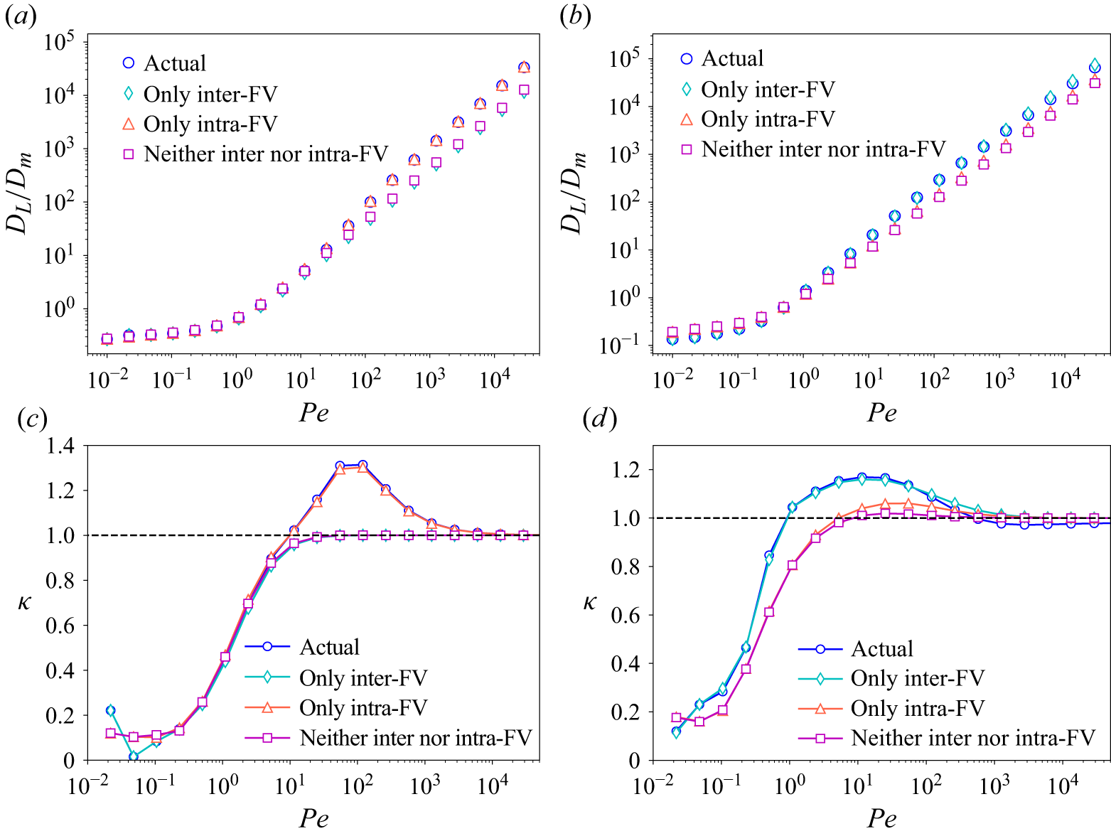
Figures 6( $a$ ) and 6( $b$ ) show how the dispersion coefficient varies with the Péclet number for two distinct tube networks, characterised by $\chi$ values of ( $a$ ) 0.1 and ( $b$ ) 1.1, respectively. For the network with $\chi = 0.1$ , the actual dispersion coefficient, which incorporates both intra-pore and inter-pore flow variability, closely matches the value obtained by considering only intra-pore flow variability. In contrast, for the network with $\chi = 1.1$ , the actual dispersion coefficient is nearly identical to the value obtained by considering only inter-pore flow variability.

Figure 6.

( $a$ , $b$ ) Dependence of the dispersion coefficient on the Péclet number as predicted by network simulations. ( $c$ , $d$ ) Relationship between the rate of change in the logarithm of the dispersion coefficient, $\kappa$ , with respect to the Péclet number. The left column illustrates results for a network with $\chi =0.1$ , whereas the right column presents data for a network with $\chi =1.1$ . A superlinear increase in the dispersion coefficient with the Péclet number is indicated when $\kappa \gt 1$ . The label ‘Actual’ refers to the actual hydrodynamic dispersion, where the network model incorporates both intra-pore and inter-pore flow variability. The labels ‘Only inter-FV’ and ‘Only intra-FV’ represent scenarios where the network model incorporates exclusively inter-pore flow variability or exclusively intra-pore flow variability, respectively. The label ‘Neither inter nor intra-FV’ indicates cases where neither inter-pore nor intra-pore flow variability is included in the model.

To quantify the scaling behaviour of the dispersion coefficient with respect to the Péclet number, we define the parameter $\kappa$ as the rate of change between the logarithm of the dispersion coefficient and the logarithm of the Péclet number, represented by

(4.3) \begin{align} \kappa = \frac {\varDelta \log (D_L / D_m)}{\varDelta \log ({Pe})}. \end{align}

A superlinear increase in the dispersion coefficient to the Péclet number is indicated when $\kappa \gt 1$ .

For actual hydrodynamic dispersion, which accounts for both intra-pore and inter-pore flow variability, the value of $\kappa$ increases with the Péclet number. After reaching a peak value, $\kappa$ begins to decrease and eventually stabilises at a plateau around one, indicating a superlinear scaling relationship between the dispersion coefficient and the Péclet number.

For the network with $\chi = 0.1$ , the $\kappa \sim {Pe}$ curve for actual hydrodynamic dispersion closely matches that when only intra-pore flow variability is considered (figure 6 $c$ ). In contrast, for the network with $\chi = 1.1$ , the $\kappa \sim {Pe}$ curve for actual hydrodynamic dispersion aligns closely with the curve when only inter-pore flow variability is considered (figure 6 $d$ ). These findings are consistent with the theoretical predictions presented in § 2, which suggest that for $\chi \gt 1$ , inter-pore flow variability primarily drives the superlinear scaling behaviour, whereas for $0 \lt \chi \lt 1$ , intra-pore flow variability dominates.

Due to the finite size of the tube networks employed in this study, the asymptotic scaling ${D_L} / {D_m} \sim {Pe} \ln ({Pe})$ is not fully achieved at high Péclet numbers (see figure 6 c). Even with networks as large as computationally feasible, hydrodynamic dispersion may remain pre-asymptotic once the Péclet number exceeds a critical threshold of ${\textit{Pe}}_c \approx 10^3$ . For ${\textit{Pe}} \lt {\textit{Pe}}_c$ , however, the results already highlight the significant impact of intra-pore flow variability on the observed superlinear scaling. Consequently, while the finite network size constrains the range over which the asymptotic regime can be observed, it does not compromise the validity of the primary conclusions.

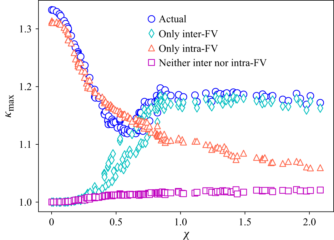
To provide a more generalised perspective, we extract the maximum value of $\kappa$ , denoted as $\kappa _{\textit{max}}$ , from the $\kappa \sim {Pe}$ curves for all the tube networks. Figure 7 illustrates how $\kappa _{\textit{max}}$ varies with $\chi$ . At low values of $\chi$ , $\kappa _{\textit{max}}$ for actual hydrodynamic dispersion closely matches that when only intra-pore flow variability is considered. This suggests that intra-pore flow variability dominates the superlinear scaling behaviour in this scenario. However, as $\chi$ increases, this trend reverses: the $\kappa _{\textit{max}}$ for actual hydrodynamic dispersion becomes almost identical to that when considering only inter-pore flow variability. At this stage, inter-pore flow variability dominates the superlinear scaling behaviour. The transition between these two opposing trends occurs at approximately $\chi \approx 0.7$ , which is in close agreement with the theoretical threshold of $\chi = 1$ . Furthermore, figure 7 indicates that, when both intra-pore and inter-pore flow variabilities are excluded, $\kappa _{\textit{max}}$ approaches one, signifying minimal superlinear scaling behaviour in this scenario. This indicates that both intra-pore and inter-pore flow variabilities are the primary sources driving the superlinear scaling relationship. Therefore, this study provides a comprehensive explanation of the mechanisms underlying the superlinear scaling of hydrodynamic dispersion.

Figure 7.

The relationship between $\kappa _{\textit{max}}$ and the parameter $\chi$ as predicted by network simulations across diverse networks. The parameter $\chi$ is calculated using (2.30). As the parameter $\chi$ increases, the primary mechanism driving superlinear scaling shifts from intra-pore flow variability to inter-pore flow variability. This transition occurs around $\chi \approx 0.7$ , which closely aligns with the theoretical threshold of $\chi = 1$ . The label ‘Actual’ refers to the actual hydrodynamic dispersion, where the network model incorporates both intra-pore and inter-pore flow variability. The labels ‘Only inter-FV’ and ‘Only intra-FV’ represent scenarios where the network model incorporates exclusively inter-pore flow variability or exclusively intra-pore flow variability, respectively. The label ‘Neither inter nor intra-FV’ indicates cases where neither inter-pore nor intra-pore flow variability is included in the model.

The findings of this study also clarify the contradictions in previous studies regarding the mechanism of superlinear scaling in hydrodynamic dispersion. These discrepancies stem from the use of structures with varying degrees of heterogeneity, leading to significantly different values of $\chi$ . This, in turn, affects the relative contributions of intra-pore and inter-pore flow variability. For instance, both Bijeljic & Blunt (Reference Bijeljic and Blunt2006) and Torelli (Reference Torelli1972) employed pore network models integrated with particle tracking to investigate hydrodynamic dispersion in tube networks with square lattice arrangements, oriented at a 45 $^{\circ }$ angle to the flow direction. Despite the similarities in model set-up, their conclusions diverged: Bijeljic & Blunt (Reference Bijeljic and Blunt2006) concluded that inter-pore flow variability dominated the superlinear scaling law, whereas Torelli (Reference Torelli1972) attributed the dominance to intra-pore flow variability. These conflicting results can be explained by differences in how structural disorder was incorporated into the models: Bijeljic & Blunt (Reference Bijeljic and Blunt2006) mapped the pore size distribution of Berea sandstone onto the network, whereas Torelli (Reference Torelli1972) randomly removed 11 % of the network nodes. As a result, the $\chi$ values for their models differed significantly, with values of 1.2 and 0.4 for Bijeljic & Blunt (Reference Bijeljic and Blunt2006) and Torelli (Reference Torelli1972), respectively. According to the transition analysis presented in § 2, these contradictory results are consistent with theoretical expectations, as the $\chi$ values for the two models are larger and smaller than 1, respectively. Furthermore, our network simulations, conducted using the same tube network, confirm the results of both studies. Detailed results of the simulations can be found in the Supplementary Material.

In this study, although both the theoretical model and PNM simulations successfully capture the transition of superlinear scaling behaviours in hydrodynamic dispersion, several limitations should be acknowledged. (i) Both the theoretical model and PNM assume zero pore volume, implying complete mixing of solute within each pore. This assumption, however, does not always hold in practice, as mixing inside individual pores is often incomplete – especially under high Péclet number conditions (Dentz et al. Reference Dentz, Le Borgne, Englert and Bijeljic2011). Nonetheless, Mehmani, Oostrom & Balhoff (Reference Mehmani, Oostrom and Balhoff2014) demonstrated that, for longitudinal dispersion in three-dimensional disordered porous media, the influence of incomplete intra-pore mixing on solute concentrations predicted by PNM is minor, with relative errors below $7\,\%$ . Therefore, although the zero-pore-volume assumption represents an idealisation, its impact on the present results is limited and acceptable. (ii) The theoretical model assumes that all tubes possess circular cross-sections, whereas pore throats in real porous media typically exhibit highly irregular geometries. Variations in cross-sectional shape not only alter local velocity distributions but also contribute to inter-pore flow variability. This simplification prevents the current model from capturing these effects on superlinear scaling behaviours in hydrodynamic dispersion. Future work could parameterise the influence of cross-sectional irregularity and explicitly incorporate it into (2.8) to (2.10), thereby extending the applicability of the $\chi$ -based theoretical framework. (iii) No PNM simulations for scenarios with $0 \lt \theta \lt 0.8$ in tube networks with high $\zeta _{\textit{max}} / \zeta _{\textit{min}}$ ratios were conducted, primarily due to the significant computational resources required to reach the asymptotic dispersion regime. Although the network model employed in this research exhibited considerable computational efficiency, the costs associated with these simulations remain prohibitive. Nevertheless, the available PNM results already provide strong evidence supporting the reliability of the $\chi$ -based model. (iv) The present study focuses exclusively on macroscopically homogeneous porous media. In heterogeneous porous structures, solute transport often exhibits anomalous behaviour (Dentz et al. Reference Dentz, Cortis, Scher and Berkowitz2004, Reference Dentz, Comolli, Hakoun and Hidalgo2020; Sahimi Reference Sahimi2012; Kang et al. Reference Kang, Lei, Dentz and Juanes2019; Puyguiraud, Gouze & Dentz Reference Puyguiraud, Gouze and Dentz2019; Andrés et al. Reference Andrés, Dentz and Cueto-Felgueroso2024; Yu et al. Reference Yu, Dentz, Sun and Zhang2024; Yin et al. Reference Yin, Man, Zhang and Galindo-Torres2024), which cannot be adequately described using a conventional dispersion coefficient.