


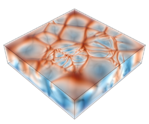



1. Introduction
Convection in porous media has attracted significant attention in recent decades owing to its huge relevance to geological carbon dioxide (CO $_2$) sequestration (Ennis-King & Paterson Reference Ennis-King and Paterson2003; Riaz & Cinar Reference Riaz and Cinar2014; Hewitt Reference Hewitt2020), which is considered one of the most promising approaches to reduce CO
 $_2$ concentration in the atmosphere (Teng & Zhang Reference Teng and Zhang2018). In brief, the captured carbon dioxide is compressed into the supercritical state and then injected into deep saline aquifers, typically regarded as porous media saturated with brine at depths greater than
 $800\ \mathrm {m}$ (Bachu Reference Bachu2000). Huppert & Neufeld (Reference Huppert and Neufeld2014) has reviewed fluid mechanics involved in this geological sequestration. Upon injection, CO
 $_2$ migrates due to buoyancy and partially dissolves into brine, leading to the formation of denser CO
 $_2$-saturated brine. Gravity-induced instability at these interfaces further evolves into convection, which in turn increases CO
 $_2$ dissolution. The dissolution and convection in porous media are important mechanisms for the stable long-term storage of underground carbon dioxide (Ennis-King & Paterson Reference Ennis-King and Paterson2003; Teng & Zhang Reference Teng and Zhang2018; Hewitt Reference Hewitt2020).
In geological formations, the brine in reservoirs commonly experiences unstable geothermal gradients in a range of  $20\unicode{x2013}65\,^\circ \mathrm {C}\ \mathrm {km}^{-1}$ (Bachu Reference Bachu2003; Nordbotten, Celia & Bachu Reference Nordbotten, Celia and Bachu2005; Hu, Xu & Yang Reference Hu, Xu and Yang2023). Meanwhile, the permeability of porous media is not always homogeneous and has a spatial distribution, which is empirically assumed to be log-normal (Chen, Zeng & Shi Reference Chen, Zeng and Shi2013). The present study consists of three-dimensional (3-D) numerical simulations of double-diffusive convection (DDC) with both gravitationally unstable temperature and concentration gradients. Both homogeneous and heterogeneous permeability are investigated. The principal objectives are to reveal the influences of geothermal gradients and heterogeneous permeability on flow structures and concentration transfer.
The underground reservoirs are modelled by two parallel horizontal plates, representing impermeable cap rock layers, with saturated porous media inside. Two typical configurations of boundary conditions have been applied in previous studies of single-phase convective dissolution in porous media (Hewitt Reference Hewitt2020). One is time-evolving one-sided convection with a fixed concentration at the top and no concentration flux at the bottom, commonly referred to as convective dissolution. The other is statistically stable two-sided convection with fixed temperature (or concentration) at the upper and lower boundaries, commonly known as Rayleigh–Darcy convection (RDC) or single-component convection. In homogeneous porous media, transient behaviours of convective fingers and variations of concentration flux over time have been studied extensively in one-sided convection (Xu, Chen & Zhang Reference Xu, Chen and Zhang2006; Hewitt, Neufeld & Lister Reference Hewitt, Neufeld and Lister2013). The dissolution rate is categorised into different regimes as time progresses (Slim Reference Slim2014), and eventually enters a decaying shutdown regime (Hewitt et al. Reference Hewitt, Neufeld and Lister2013). Two-sided convection focuses on the influence of driving force, i.e. Rayleigh number  ${Ra}$, on dominant flow structures and heat (or concentration) flux. Previous studies have revealed that the scaling between the flux
 ${Nu}$ and
 ${Ra}$ varies across different
 ${Ra}$ ranges. Otero et al. (Reference Otero, Dontcheva, Johnston, Worthing, Kurganov, Petrova and Doering2004) conducted two-dimensional (2-D) numerical simulations and found
 ${Nu}\sim {Ra}$ over an intermediate range
 $50\lesssim {Ra}\lesssim 1200$ and
 ${Nu}\sim {Ra}^{0.9}$ from
 $1255$ to
 $10^4$. Hewitt, Neufeld & Lister (Reference Hewitt, Neufeld and Lister2012) found a similar scaling
 ${Nu}\sim {Ra}^{0.95}$ in high-
 ${Ra}$ range
 $1300\lesssim {Ra} \le 4\times 10^4$ in 2-D simulations. Later, Hewitt, Neufeld & Lister (Reference Hewitt, Neufeld and Lister2014) extended simulations to 3-D cases and observed a fitted linear scaling
 ${Nu}=0.0096{Ra}+4.6$ in the range
 $1750\le {Ra}\le 2\times 10^4$. More recently, Pirozzoli et al. (Reference Pirozzoli, De Paoli, Zonta and Soldati2021) and De Paoli et al. (Reference De Paoli, Pirozzoli, Zonta and Soldati2022) have pushed Rayleigh number up to a large value of
 $8\times 10^4$, adding a sublinear corrective term that only influences moderate
 ${Ra}$ values. Zhu, Fu & De Paoli (Reference Zhu, Fu and De Paoli2024) proposed a possible explanation for this additional nonlinear term. The size of flow structures can be measured by the wavenumber, which follows a fitted scaling
 ${Ra}^{0.4}$ in 2-D simulations (Hewitt et al. Reference Hewitt, Neufeld and Lister2012) and approximately
 ${Ra}^{0.5}$ in 3-D simulations (Hewitt et al. Reference Hewitt, Neufeld and Lister2014; De Paoli et al. Reference De Paoli, Pirozzoli, Zonta and Soldati2022).
Early studies of DDC in homogeneous porous media focused on the onset of convection. Using linear stability analysis, Nield (Reference Nield1968) obtained critical Rayleigh numbers and corresponding critical wavenumbers under various boundary conditions of temperature and concentration. Taunton, Lightfoot & Green (Reference Taunton, Lightfoot and Green1972) extended the analysis to determine conditions for salt fingers. Anisotropic permeability and diffusion coefficients were further considered by Tyvand (Reference Tyvand1980) to investigate thermohaline instability. The above studies used Darcy's law to determine the seepage velocity. Instability of flows described by a Brinkman model has also been explored (Wang & Tan Reference Wang and Tan2009; Prakash & Gupta Reference Prakash and Gupta2012). In numerical simulations, Trevisan & Bejan (Reference Trevisan and Bejan1987) considered the buoyancy effect solely by temperature gradient in 2-D porous media and obtained a scaling law of mass transfer rate for various Lewis numbers. Laboratory experiments were carried out by Griffiths (Reference Griffiths1981) who measured the heat and salt fluxes through interfaces in a two-layer convecting system in a Hele-Shaw cell. Murray & Chen (Reference Murray and Chen1989) considered the onset of DDC in a finite box of porous medium. Persistent investigations into DDC in porous media encompass various aspects, including horizontal throughflow (Rubin & Roth Reference Rubin and Roth1979), vertical vibration (Jounet & Bardan Reference Jounet and Bardan2001), mechanical dispersion (Rosenberg & Spera Reference Rosenberg and Spera1992), heat-releasing concentration (Hill Reference Hill2005) and nonlinear stability (Lombardo, Mulone & Straughan Reference Lombardo, Mulone and Straughan2001). Comprehensive reviews of DDC in porous media have been conducted by Trevisan & Bejan (Reference Trevisan and Bejan1990), Vafai (Reference Vafai2005) and Nield & Bejan (Reference Nield and Bejan2017). In our recent study (Hu et al. Reference Hu, Xu and Yang2023), we systematically investigated the effects of unstable geothermal gradients on the one-sided convection. It has been addressed that large-scale rolls induced by the geothermal gradient can significantly influence flow structures and dissolution rates. The long-term variation of dissolution flux over time exhibits consistent decaying behaviour and can be modelled by a theoretical relation.
Another important factor to consider is permeability heterogeneity quantified by the Dykstra–Parsons coefficient  $V_{DP}$, which ranges from
 $0$, indicating perfect homogeneity, to
 $1$, signifying maximum heterogeneity. Buoyancy-driven convection in heterogeneous porous media has been investigated theoretically, numerically and experimentally. The effects of heterogeneity on the onset of convection in porous media have been discussed extensively in a series of studies (Nield & Kuznetsov Reference Nield and Kuznetsov2007a,Reference Nield and Kuznetsovb; Nield, Kuznetsov & Simmons Reference Nield, Kuznetsov and Simmons2010; Nield & Kuznetsov Reference Nield and Kuznetsov2011). Braester & Vadasz (Reference Braester and Vadasz1993) utilised a perturbation expansion method to study weak heterogeneity. Heterogeneous permeability can be generated by many methods. For instance, Soboleva (Reference Soboleva2018) introduced inhomogeneity using multiple horizontal layers at different porosity and permeability. Mahyapour et al. (Reference Mahyapour, Mahmoodpour, Singh and Omrani2022) employed the sequential Gaussian simulation method to produce random permeability fields and studied the effects of permeability heterogeneity on one-sided convective dissolution. Farajzadeh et al. (Reference Farajzadeh, Ranganathan, Zitha and Bruining2010) used spectral methods to generate 2-D fields with various correlation lengths and
 $V_{DP}$. They concluded three flow regimes (fingering, dispersive and channeling) for density-driven natural convection flow through numerical simulations, which adopts the ideas of Waggoner, Castillo & Lake (Reference Waggoner, Castillo and Lake1992), and found the heterogeneity is not related to the mass of dissolved CO
 $_2$. Similar results were given by Ranganathan et al. (Reference Ranganathan, Farajzadeh, Bruining and Zitha2012). However, an increase in total dissolved CO
 $_2$ with heterogeneity was observed by Kong & Saar (Reference Kong and Saar2013). Experimental set-ups include a sloping permeability jump in a saturated two-layered porous medium (Bharath & Flynn Reference Bharath and Flynn2021), a Hele-Shaw cell with a thin horizontal layer of circular impermeable discs (Salibindla et al. Reference Salibindla, Subedi, Shen, Masuk and Ni2018) and packed stratified plastic resin particles with different average diameter (Wang et al. Reference Wang, Nakanishi, Hyodo and Suekane2017). As for DDC, Kuznetsov & Nield (Reference Kuznetsov and Nield2008, Reference Kuznetsov and Nield2012) analytically studied the onset of convection using linear stability theory. Islam, Lashgari & Sephernoori (Reference Islam, Lashgari and Sephernoori2014b) numerically investigated 2-D convective dissolution with geothermal gradients. Results revealed that dissolution is enhanced with increasing both solutal Rayleigh number and heterogeneity level, and the geothermal effect has a minor effect on overall dissolution process.
The rest of the paper is organised as follows. In § 2, we describe the governing equations and corresponding numerical methods, as well as the control parameter spaces and methods for generating heterogeneous permeability fields. In § 3, we analyse numerical results of DDC in homogeneous porous media, including flow structures and fluxes. In § 4, we focus on variations of permeability heterogeneity in both RDC and DDC. Finally, we summarise our results in § 5.
2. Methodology
2.1. Governing equations
In a Cartesian coordinate  $\boldsymbol {x}=(x,y,z)$, we consider a 3-D cell containing fluid-saturated porous media bounded by two horizontal plates with a uniform porosity
 $\phi$. The cell has a height of
 $H$, and its length and width are both
 $L$. The permeability of porous media is either homogeneous, characterised by a constant value
 $\bar {K}$, or heterogeneous, defined by a spatial function
 $K(\boldsymbol {x})=\bar {K}f(\boldsymbol {x})$ following a certain distribution. Here
 $f(\boldsymbol {x})$ is a normalised function to describe permeability heterogeneity, with an average value of unity over the entire domain. Note that the permeability is generally considered a second-order tensor with anisotropy in the horizontal and vertical directions (Rapaka et al. Reference Rapaka, Pawar, Stauffer, Zhang and Chen2009; Green & Ennis-King Reference Green and Ennis-King2014; De Paoli, Zonta & Soldati Reference De Paoli, Zonta and Soldati2017; Nield & Bejan Reference Nield and Bejan2017). For simplicity, we assume isotropic permeability in this study. The details of generating a heterogeneous permeability field are discussed in the following section. The cell is maintained at a constant concentration at the top and zero concentration at the bottom. Meanwhile, there is a consistent unstable geothermal gradient across the domain against the direction of gravity. In other words, the saturated porous media are heated from below and cooled from above. We denote concentration and temperature as
 $S$ and
 $T$, respectively. The top and bottom boundaries are marked with subscripts ‘
 $top$’ and ‘
 $bot$’, respectively. The density of fluid follows a linear relation as
 $\rho =\rho _0[1-\beta _{T} (T-T_{top})+\beta _{S} (S-S_{bot})]$, where
 $\beta _{T}$ and
 $\beta _{S}$ are linear coefficients of expansion and
 $\rho _0$ is a reference value. The governing equations of an incompressible Darcian flow with both heat and mass transfer read
 $$\begin{gather} \boldsymbol{\nabla} \boldsymbol{\cdot} \boldsymbol{u} = 0 , \end{gather}$$
 $$\begin{gather}\boldsymbol{u} ={-}\frac{K(\boldsymbol{x})}{\mu}[\boldsymbol{\nabla} p+(\beta_{S} S - \beta_{T} T) \rho_{0} g \boldsymbol{e}_{z}] , \end{gather}$$
 $$\begin{gather}\frac{(\rho c)_{m}}{(\rho c_{p})_{f}}\frac{\partial T}{\partial t} ={-}\boldsymbol{u} \boldsymbol{\cdot} \boldsymbol{\nabla} T+\kappa_{m} \nabla^{2} T , \end{gather}$$
 $$\begin{gather}\phi \frac{\partial S}{\partial t} ={-}\boldsymbol{u} \boldsymbol{\cdot} \boldsymbol{\nabla} S+\phi \kappa_{S} \nabla^{2} S. \end{gather}$$
Here  $\boldsymbol {u}$ is the seepage velocity,
 $p$ is the pressure,
 $g$ is the gravitational acceleration,
 $\boldsymbol {e}_z$ is the vertical unit vector opposite to direction of gravity,
 $\mu$ is fluid viscosity,
 $(\rho c)_{m}$ is the overall heat capacity of solid and fluid,
 $(\rho c_{p})_{f}$ is the heat capacity of fluid,
 $\kappa _m$ is the overall thermal diffusivity and
 $\kappa _{S}$ is the molecular diffusivity of concentration field, respectively. The subscript ‘
 $m$’ represents the combination of both the solid matrix and saturated fluid, whereas ‘
 $f$’ represents the fluid alone. Note that local thermal equilibrium is assumed in (2.1c). Periodicity is imposed on the horizontal directions, namely, the
 $x$ and
 $y$ dimensions, for all variables. The boundary conditions at the bottom and top boundaries are
 $$\begin{gather} u_z = 0,\quad T = T_{bot},\quad S = S_{bot},\quad \mbox{at}\ z=0, \end{gather}$$
 $$\begin{gather}u_z = 0,\quad T = T_{top},\quad S = S_{top},\quad \mbox{at}\ z=H. \end{gather}$$
The above governing equations are non-dimensionalised by the height  $H$, the temperature difference
 $\Delta T=T_{bot}-T_{top}$, the concentration difference
 $\Delta S=S_{top}-S_{bot}$, the characteristic velocity
 $U_c=\bar {K}g\rho _0\beta _{S} \Delta S / \mu$, and the characteristic time scale
 $t_c = \phi H / U_c$, respectively. Then the non-dimensionalised equations are
 $$\begin{gather} \boldsymbol{\nabla} \boldsymbol{\cdot} \boldsymbol{u} = 0 , \end{gather}$$
 $$\begin{gather}\boldsymbol{u} = [-\boldsymbol{\nabla} p+ (\varLambda T -S)\boldsymbol{e}_z]f(\boldsymbol{x}), \end{gather}$$
 $$\begin{gather}\sigma \frac{\partial T}{\partial t} ={-}\boldsymbol{u} \boldsymbol{\cdot} \boldsymbol{\nabla} T+ \frac{Le}{{Ra}_S}\nabla^{2} T , \end{gather}$$
 $$\begin{gather}\frac{\partial S}{\partial t} ={-}\boldsymbol{u} \boldsymbol{\cdot} \boldsymbol{\nabla} S+ \frac{1}{{Ra}_S}\nabla^{2} S . \end{gather}$$
In the remainder of this article, all variables are dimensionless unless otherwise mentioned. Note that both the temperature and concentration differences are positive, which means the two scalars simultaneously drive convective motions.
There are four dimensionless control parameters in the above equations, including the heat capacity ratio  $\sigma$, the Lewis number
 ${Le}$, the concentration Rayleigh number
 ${Ra}_S$ and the temperature Rayleigh number
 ${Ra}_T$, which are respectively defined as
 \begin{align} \sigma = \frac{(\rho
c)_m}{\phi(\rho c_p)_f}, \quad {Le} =
\frac{\kappa_m}{\phi\kappa_S}, \quad {Ra}_S =
\frac{\bar{K}Hg\rho_0\beta_S \Delta S}{\kappa_S \mu \phi},
\quad {Ra}_T = \frac{\bar{K}Hg\rho_0\beta_T \Delta
T}{\kappa_m\mu}.
\end{align}
The density ratio  $\varLambda =(\beta _T\Delta T)/(\beta _S \Delta S) = {Ra}_T {Le} / {Ra}_S$ can be assembled to measure the strength of the temperature difference relative to the concentration difference. The non-dimensionalised boundary conditions at the bottom and top boundaries then become
 $$\begin{gather} u_z = 0,\quad T = 1,\quad S = 0,\quad \mbox{at}\ z=0, \end{gather}$$
 $$\begin{gather}u_z = 0,\quad T = 0,\quad S = 1,\quad \mbox{at}\ z=1. \end{gather}$$
2.2. Permeability heterogeneity
Before solving the governing equations, the heterogeneous permeability field must be properly generated as a reflection of realistic geological formations. Permeability in natural geological formations is empirically assumed to follow a log-normal distribution. Thus, the normalised permeability function  $f(\boldsymbol {x})$ is modelled by the exponential of a random Gaussian field
 $G(\boldsymbol {x})$ which has zero mean and unit standard deviation (Oliver Reference Oliver1995; Camhi, Meiburg & Ruith Reference Camhi, Meiburg and Ruith2000; Abrahamsen, Kvernelv & Barker Reference Abrahamsen, Kvernelv and Barker2018). The autocovariance function of
 $G(\boldsymbol {x})$ is given as
 $C(\boldsymbol {x})=\exp (-({\boldsymbol {x}}/{l_r})^2)$ where
 $l_r$ denotes the non-dimensionalised correlation length. We use the Dykstra–Parsons coefficient
 $V_{DP}$ to measure the strength of heterogeneity. When permeability is log-normally distributed,
 $V_{DP}$ can be expressed as
 $V_{DP}=1-\mathrm {e}^{-s_{\ln {k}}}$, where
 $s_{\ln {k}}$ is the standard deviation of logarithmic
 $f(\boldsymbol {x})$ (Kong & Saar Reference Kong and Saar2013). Consequently, the normalised permeability function
 $f(\boldsymbol {x})$ can be expressed as
 \begin{equation} f(\boldsymbol{x})=\exp\left(-\frac{s^2_{\ln{k}}}{2}+s_{\ln{k}}G\right). \end{equation}
2.3. Numerical details
To numerically solve the governing equations (2.3) with boundary conditions (2.5), we first take the divergence of (2.3b) and combine it with continuity equation (2.3a). An equation for pressure can be obtained as
 \begin{equation} \boldsymbol{\nabla}\boldsymbol{\cdot}(f\boldsymbol{\nabla} p) = \frac{\partial}{\partial z}[(\varLambda T-S)f], \end{equation}
with boundary conditions as
 \begin{equation} \left.\frac{\partial p}{\partial z}\right|_{z=0,1} = (\varLambda T-S)|_{z=0,1}. \end{equation}
For homogeneous porous media,  $f(\boldsymbol {x})$ equals one in the entire domain. Equation (2.7) reduces into a Poisson's equation, which can be solved by the same numerical method as described in Hu et al. (Reference Hu, Xu and Yang2023). Specifically, apply Fourier transform in the horizontal directions and solve a set of tridiagonal systems in the vertical direction. However,
 $f(\boldsymbol {x})$ becomes spatially dependent when considering heterogeneity. Equation (2.7) is generally a Poisson's equation with variable coefficients and can no longer be solved by a fast direct algorithm. Therefore, an iterative V-cycle multigrid method is employed (Briggs, Henson & McCormick Reference Briggs, Henson and McCormick2000). The iteration stops when the divergence of velocity field is less than
 $10^{-6}$. After solving the pressure field, the velocity can be calculated using (2.3b). The advection–diffusion equations for temperature and concentration can then be solved by the scheme described in Ostilla-Mónico et al. (Reference Ostilla-Mónico, Yang, Van Der Poel, Lohse and Verzicco2015). Initially, the concentration and temperature fields have vertically linear distributions based on their boundary values.
In this study, the Lewis number and heat capacity ratio are fixed at  $Le=100$ and
 $\sigma =1$, respectively. The parameter spaces are shown in figure 1. For homogeneous porous media, we explore four concentration Rayleigh numbers ranging from
 $10^3$ to
 $10^4$ and six temperature Rayleigh numbers ranging from zero, i.e. without geothermal gradient, to
 $300$. The Rayleigh numbers fall within ranges estimated by Hu et al. (Reference Hu, Xu and Yang2023) for realistic conditions in CO
 $_2$ sequestration, with the concentration Rayleigh number up to
 $10^5$ and the temperature Rayleigh number as high as
 $10^3$. For heterogeneous cases, we fix the concentration Rayleigh number at
 $10^3$ and the temperature Rayleigh numbers at zero or
 $50$. The two parameters concerning heterogeneity are correlation length
 $l_r$, ranging from
 $0.1$ to
 $1.0$, and the Dykstra–Parsons coefficient
 $V_{DP}$, ranging from
 $0.1$ to
 $0.6$. Previous studies on permeability heterogeneity in porous media in the context of CO
 $_2$ sequestration have considered various ranges of the Dykstra–Parsons coefficient and correlation length (Waggoner et al. Reference Waggoner, Castillo and Lake1992; Jensen et al. Reference Jensen, Lake, Corbett and Goggin1997; Camhi et al. Reference Camhi, Meiburg and Ruith2000; Farajzadeh et al. Reference Farajzadeh, Ranganathan, Zitha and Bruining2010; de Dreuzy et al. Reference de Dreuzy, Carrera, Dentz and Le Borgne2012; Ranganathan et al. Reference Ranganathan, Farajzadeh, Bruining and Zitha2012; Kong & Saar Reference Kong and Saar2013; Islam et al. Reference Islam, Korrani, Sepehrnoori and Patzek2014a,Reference Islam, Lashgari and Sephernoorib). To conclude,
 $V_{DP}$ and
 $l_r$ vary in the ranges
 $0.01 \le V_{DP} \le 0.9$ and
 $0.01 \le l_r \le 3$, respectively. Therefore, the parameters explored in this study are representative of realistic conditions.
Parameter spaces for (a) homogeneous and (b) heterogeneous porous media. Note that we set  ${Ra}_S=10^3$ and
 ${Ra}_T=0$ or
 $50$ in heterogeneous porous media.

3. Homogeneous porous media
In the context of convection in homogeneous porous media, our major concern is how the geothermal gradient influences flow dynamics and transport properties compared with convection in the absence of such a gradient. To examine such influences, we conduct numerical simulations in the concentration Rayleigh number range  $10^3 \le {Ra}_S \le 10^4$. For each
 ${Ra}_S$, the temperature Rayleigh number ranges from
 $0 \le {Ra}_T \le 300$. Note that the critical Rayleigh number for single-component RDC is
 $Ra_{cr}=4{\rm \pi} ^2$ (Lapwood Reference Lapwood1948), which is slightly less than 40. An instinctual assumption is that the temperature gradient barely influences the flow when
 ${Ra}_T$ is less than
 $Ra_{cr}$. In this circumstance, temperature is more like a passive scalar driven by concentration convective motions.
3.1. Alternation of flow structures
3.1.1. Root-mean-square of velocity field  $u^{rms}$

We first look at the time- and volume-averaged root-mean-square (r.m.s.) of velocity field  $u^{rms}$ as shown in figure 2. The observation in figure 2(a) is evident that
 $u^{rms}$ shows no significant change for
 ${Ra}_T=0$ and
 $10$ regardless of
 ${Ra}_S$. However, when considering a constant concentration Rayleigh number,
 $u^{rms}$ demonstrates an approximately linear escalation with increasing
 ${Ra}_T$ for values exceeding
 $40$. It is noteworthy that the slope differs for various
 ${Ra}_S$ values. For clarification, the observed decrease in
 $u^{rms}$ with increasing
 ${Ra}_S$ at a fixed temperature Rayleigh number is due to the non-dimensionalisation of variables used in our study. The dimensional velocity should increase with stronger driving forces. Exploring the variations of
 $u^{rms}$ with the density ratio
 $\varLambda$, we observe a consistent linear trend in the data with respect to
 $\varLambda$. A linear best-fit model of
 $u^{rms}=0.115(\varLambda +1)$ is also depicted in figure 2(b). Such a linear tendency can be explained by the fact that the total driving forces of convection include density differences induced by both concentration and temperature differences. However, only concentration difference is used when non-dimensionalising the governing equations, resulting in a
 $(\varLambda +1)$ term for the non-dimensionalised
 $u^{rms}$.
Root-mean-square of time- and volume-averaged velocity varies with (a) temperature Rayleigh number  ${Ra}_T$ and (b) density ratio
 $\varLambda$. The grey dashed line in (b) is a linear fit
 $u^{rms}=0.115(\varLambda +1)$. The ratio of Péclet number
 $Pe$ to its analytical relation
 $Pe_e$ against
 ${Ra}_S$ is plotted in (c), with the grey dashed line indicating unity value.

Recently, Zhu et al. (Reference Zhu, Fu and De Paoli2024) have presented a theoretical relation for the r.m.s. of velocity  $u^{rms}$ (or the corresponding Péclet number
 $Pe$), the Nusselt number
 $Nu$ and the Rayleigh number
 $Ra$ in single-component convective porous media flows. Similarly, we can obtain a relation in the double-diffusive scenario for
 $u^{rms}$, the Nusselt and Rayleigh numbers, which reads
 \begin{equation} Pe^2={Ra}_S[\varLambda Le(Nu_T-1)+(Nu_S-1)], \end{equation}
where  $Pe= {Ra}_S u^{rms}$. The derivation details are provided in Appendix B. The ratio of numerical measurements to the theoretical relation is depicted in figure 2(c). The results demonstrate excellent agreement between the measurements and theory, both for
 ${Ra}_T = 0$ and for
 ${Ra}_T > 0$.
3.1.2. Structures of the flow
The flow structures exhibit variations with concentration and temperature Rayleigh numbers. Figure 3 presents horizontal slices of vertical velocity, concentration, and temperature at  $z=0.5$ for two concentration Rayleigh numbers. To analyse the impacts of different temperature gradients, the subfigures are organised in descending rows corresponding to increasing
 ${Ra}_T$. For a fixed
 ${Ra}_S$, it is notable that only when
 ${Ra}_T$ is greater than
 $40$ do the flow structures alter significantly. When
 ${Ra}_T=0$ and
 $10$, the concentration field comprises randomly distributed column-like structures of comparable size. In other words, the flow is almost unaffected if
 ${Ra}_T<{Ra}_{cr}$, aligning with the aforementioned assumption. However, as
 ${Ra}_T$ surpasses
 ${Ra}_{cr}$, either concentration or temperature difference can independently drive convection, while their combined effect leads to more intricate flow patterns. The concentration field displays sheet-like structures and cellular structures with elongated borders where concentration reaches maximum or minimum. The interfaces of concentration structure in horizontal directions become more distinct as
 ${Ra}_T$ increases for a fixed
 ${Ra}_S$ when
 ${Ra}_T>{Ra}_{cr}$ (see figure 3c–e).
Horizontal slices of vertical velocity, concentration and temperature at  $z=0.5$. The left three columns correspond to
 ${Ra}_S=10^3$, and the right three columns to
 ${Ra}_S=10^4$. Each row represents a temperature Rayleigh number, ranging from (a) 0 to (e) 300.

It is worth noting that the temperature structures display variations at an identical  ${Ra}_T$ when the concentration Rayleigh number differs. This suggests that the density ratio also influences the flow structures. For instance, when
 ${Ra}=10^3$ and
 ${Ra}_T=100$ (density ratio corresponding to
 $\varLambda =10$), parallel sheet-like structures prevail in the left panel of figure 3(d). The temperature field is similar to convection solely driven by temperature at
 ${Ra}_T=100$. However, when
 ${Ra}=10^4$ and
 ${Ra}_T=100$ (density ratio corresponding to
 $\varLambda =1$), parallel sheets break down and reorganise. This is due to the differing relative strengths of buoyancy induced by temperature and concentration. In the former case,
 $\varLambda =10$ indicates the flow is primarily driven by temperature difference, resulting in structures similar to those solely driven by
 ${Ra}_T=100$. In the latter case, the buoyant forces from concentration and temperature are equivalent, leading to deviations from structures of RDC driven by either
 ${Ra}_S=10^4$ or
 ${Ra}_T=100$.
Furthermore, upon comparing temperature and concentration slices under identical control parameters, it is evident that concentration structures typically concentrate in the centre of corresponding temperature structures, where the vertical velocity attains its maximum. This observation implies high concentration can be transported quickly from the top plate to the bottom in these areas and vice versa. To further illustrate such implications, vertical slices of concentration at  $y=0.5L$ for
 ${Ra}_S=10^4$ are presented in figure 4. For large
 ${Ra}_T$, the concentration structures consist of numerous short fingers emerging from the boundaries and a few long plumes extending across the entire vertical direction, reflecting the footprints of large-scale rolls induced by temperature. As
 ${Ra}_T$ increases, more and more concentration fingers are confined within a short vertical distance apart from the top and bottom boundaries, and the plumes become thinner. In addition, mixing is enhanced and concentration is more homogenised in the bulk region for increasing temperature gradient.
Vertical slices of concentration at  $y=0.5L$ for
 ${Ra}_S=10^4$: (a)
 ${Ra}_T=0$, (b)
 ${Ra}_T=10$, (c)
 ${Ra}_T=40$, (d)
 ${Ra}_T=100$, (e)
 ${Ra}_T=200$ and (f)
 ${Ra}_T=300$.

The horizontal slices in figure 3 indicate that the structure sizes vary with the Rayleigh numbers. The size of dominant structures is typically quantified by the mean radial wavenumber at the centre plane  $z=0.5$. Consider a 2-D power spectrum of the concentration slice at
 $z=0.5$,
 $E(k_x,k_y)$, where
 $k_x$ and
 $k_y$ are the wavenumbers in the
 $x$ and
 $y$ directions, respectively. The time-averaged radial wavenumber for concentration is defined as
 \begin{equation} k_{rS}=\left\langle\frac{\displaystyle\iint\sqrt{k_x^2+k_y^2}E(k_x,k_y)\,\mathrm{d}k_x \,\mathrm{d}k_y}{\displaystyle\iint E(k_x,k_y)\,\mathrm{d}k_x \,\mathrm{d}k_y}\right\rangle. \end{equation}
In 3-D RDC, numerical measurements have provided fitted scalings of  $k_r\approx 0.17Ra^{0.52}$ by Hewitt et al. (Reference Hewitt, Neufeld and Lister2014) and
 $k_r\approx 0.25Ra^{0.49}$ by De Paoli et al. (Reference De Paoli, Pirozzoli, Zonta and Soldati2022). In figure 5(a), we present the variations of
 $k_{rS}$ with both concentration and temperature Rayleigh numbers. Results from De Paoli et al. (Reference De Paoli, Pirozzoli, Zonta and Soldati2022) are also included for comparison, showing good agreement with our results at
 ${Ra}_T=0$. For the case
 ${Ra}_T=10$,
 $k_{rS}$ is nearly the same as for
 ${Ra}_T=0$ at a fixed
 ${Ra}_S$. However, when
 ${Ra}_T \ge 40$, the wavenumber does not follow the approximate 1/2 power scaling with
 ${Ra}_S$. Here, we define an effective Rayleigh number
 $Ra_e$ to indicate the total driving buoyant forces of both concentration and temperature as
 \begin{equation} Ra_e \equiv {Ra}_S+Le {Ra}_T = {Ra}_S(1+\varLambda). \end{equation}
After plotting  $k_{rS}$ against
 $Ra_e$ in a logarithmic coordinate in figure 5(b), we find that the averaged radial wavenumber exhibits a linear increase with the effective Rayleigh number. The best data fitting results in
 \begin{equation} k_{rS} \approx 0.23 Ra_e^{0.47}. \end{equation}
The fitting exponent and coefficient are close to the fitted scaling by De Paoli et al. (Reference De Paoli, Pirozzoli, Zonta and Soldati2022). Although our numerical measurements do not perfectly collapse on the best-fit line, the fitted scaling successfully captures the trend of structure size varying with the Rayleigh numbers.
The mean radial wavenumber  $k_{rS}$ of concentration field at
 $z=0.5$ against (a) the concentration Rayleigh number
 ${Ra}_S$ and (b) the effective Rayleigh number
 $Ra_e={Ra}_S+Le {Ra}_T$. The black empty circles in (a) represent 3-D numerical results from De Paoli et al. (Reference De Paoli, Pirozzoli, Zonta and Soldati2022) in single-component RDC. The grey dashed line in (b) is the best power fit
 $k_{rS}=0.23Ra_e^{0.47}$.

3.1.3. Concentration mean profiles
In figure 6 we plot the concentration mean profiles for all cases in the parameter space. The symbol angle brackets stand for an average over time and  $(x,y)$ planes. For each profile, there are two distinct boundary layers near the top and bottom plates, and the concentration is approximately linear with height in the bulk regions around the centre. For a fixed
 ${Ra}_S$, the thickness of boundary layers decreases and the concentration gradient near the centre changes from positive to negative with increasing
 ${Ra}_T$. We measure the concentration gradient
 $G_S$ in the range
 $0.4\le z \le 0.6$ and plot its dependence on
 ${Ra}_S$ and
 ${Ra}_T$ in figure 7. Then
 $G_S$ becomes negative when
 ${Ra}_T$ is larger than
 $40$ for all explored
 ${Ra}_S$. In other words, the concentration gradient in the bulk is opposite to that imposed on the vertical boundaries provided that
 ${Ra}_T$ exceeds the critical
 $Ra_{cr}$. Such a phenomenon can be attributed to the fact that increasing
 ${Ra}_T$ for a fixed
 ${Ra}_S$ is equivalent to increasing density ratio, resulting in a higher vertical velocity. Flow with high vertical velocity can transfer high concentration quickly from the top to the bottom with little diffusion, and vice versa. Consequently, the concentration gradient in the bulk becomes negative. A positive value of the concentration gradient is expected at low
 ${Ra}_T$. However, it is noteworthy that the minimum
 $G_S$ occurs at
 ${Ra}_T=10$ with two lower concentration Rayleigh numbers,
 ${Ra}_S=10^3$ and
 $2\times 10^3$. In the context of RDC, De Paoli et al. (Reference De Paoli, Pirozzoli, Zonta and Soldati2022) reported similar counter-gradient flux regions at the edge of thermal boundary layer at small Rayleigh numbers (
 ${Ra}=10^3$ in their cases), ascribing this phenomenon to vertical plumes that carry their momentum and temperature almost unchanged across the fluid layer. These regions tend to diminish with increasing
 ${Ra}$. Based on our current numerical results, we can only offer a qualitative description of this phenomenon rather than a definitive explanation. In our cases, although only a very small
 ${Ra}_T$ is introduced at
 ${Ra}_S=10^3$ and
 $2\times 10^3$, the nonlinear interaction between concentration and temperature results in extending the counter-gradient flux regions into the bulk and can significantly invert the concentration gradient.
Concentration mean profiles: (a)  ${Ra}_S=10^3$, (b)
 ${Ra}_S=2 \times 10^3$, (c)
 ${Ra}_S=5 \times 10^3$ and (d)
 ${Ra}_S=10^4$. Line colours from blue to red represent increasing temperature Rayleigh number.

Concentration gradient calculated in the range  $0.4\le z \le 0.6$.

3.2. Variation of fluxes with ${Ra}_S$ and ${Ra}_T$


The non-dimensionalised concentration flux is defined as the mean value of the vertical concentration gradient at the top and bottom boundaries:
 \begin{equation} Nu_S=\frac{1}{2}\left(\left\langle\left.\frac{\partial S}{\partial z}\right|_{z=0}+\left.\frac{\partial S}{\partial z}\right|_{z=1}\right\rangle\right), \end{equation}
where  $\langle {\cdot }\rangle$ denotes averaging over time and horizontal directions. The definition of the heat flux
 $Nu_T$ is similar. Previous studies have analysed heat or concentration transfer in 3-D single-component RDC and concluded a nearly linear scaling law
 $Nu\sim \alpha _0 Ra$ at high Rayleigh numbers in the range
 $1750\le Ra \le 2\times 10^4$ with the linear coefficient
 $\alpha _0$ around
 $0.01$ (Hewitt et al. Reference Hewitt, Neufeld and Lister2014). However, it is not always the case when considering an additional aiding temperature gradient.
3.2.1. Numerical measurements
The variance of concentration flux with  ${Ra}_S$ and
 ${Ra}_T$ is shown in figure 8. In figure 8(a), for the cases
 ${Ra}_T=0,10,40$, the linear relation can still retain for the
 ${Ra}_S$ range we explored and their curves almost collapse. For comparison, the linear relation
 $Nu_S=0.0096{Ra}_S+4.6$ given by (Hewitt et al. Reference Hewitt, Neufeld and Lister2014) is also depicted in figure 8(a). This indicates that when the temperature Rayleigh number is small, it merely influences concentration flux. However, for the cases
 ${Ra}_T=100$,
 $200$ and
 $300$, the variations with
 ${Ra}_S$ are clearly nonlinear, with an elevation at two smaller concentration Rayleigh numbers
 ${Ra}_S=10^3$ and
 $2\times 10^3$. In figure 8(b), the fluxes for two higher
 ${Ra}_S$ do not change significantly. However, for two lower
 ${Ra}_S=10^3$ and
 $2\times 10^3$, the fluxes increase linearly with
 ${Ra}_T$ and is nearly independent of
 ${Ra}_S$ when temperature Rayleigh number exceeds
 $100$. As a result, the fluxes change remarkably only when concentration Rayleigh number is small and temperature Rayleigh number is large compared with RDC without a temperature gradient. In other words, the flux increment is highly related to the density ratio. After rescaling concentration flux with the effective Rayleigh number
 ${Ra}_e$ in figure 9, we find that it decreases with density ratio and asymptotically attains a constant value. This asymptote will be explained by the scale analysis in the following section.
The variance of concentration flux with (a) concentration Rayleigh number and (b) temperature Rayleigh number. The grey dashed line in (a) indicates a linear relation obtained by Hewitt et al. (Reference Hewitt, Neufeld and Lister2014) in 3-D RDC.

The variation of (a) concentration and (b) heat flux rescaled by the effective Rayleigh number with density ratio. The grey dashed lines are (3.6a–d) given by scale analysis.

3.2.2. Scale analysis for concentration-dominant and temperature-dominant flow
Examine two contrasting scenarios with both high- ${Ra}_S$ and
 ${Ra}_T$ characterised by the density ratio, with one corresponding to the concentration-dominant regime where
 $\varLambda \ll 1$ and the other to the temperature-dominant regime with
 $\varLambda \gg 1$. In the former case, the dominant driving forces for the flow are concentration, while in the latter, temperature takes precedence.
The concentration-dominant flow in the boundary layers is featured by the horizontal and vertical length scales as  $x(\mathrm {or}\ y)\sim H$ and
 $z\sim \delta _S$, respectively. The scales of the velocity are
 $(U,V,W)$. The scale equivalences recommended by the governing equations are
 \begin{equation} \frac{U}{H}\sim\frac{W}{\delta_S},\quad W\sim\frac{Kg \Delta \rho_S^\ast}{\mu},\quad U\frac{\Delta T^\ast}{H}\sim\kappa_T \frac{\Delta T^\ast}{\delta_T^2},\quad W\frac{\Delta S^\ast}{\delta_S}\sim\phi\kappa_S\frac{\Delta S^\ast}{\delta_S^2}. \end{equation}
The above equivalences can yield
 \begin{equation} Nu_{S1}\sim\frac{\delta_S}{H}\sim {Ra}_S,\quad Nu_{T1}\sim\frac{\delta_T}{H} \sim {Ra}_S Le^{{-}1/2}. \end{equation}
Similarly, the scale equivalences for temperature-dominant flow are
 \begin{equation} \frac{U}{H}\sim\frac{W}{\delta_T},\quad W\sim\frac{Kg \Delta \rho_T^\ast}{\mu},\quad U\frac{\Delta T^\ast}{H}\sim\kappa_T\frac{\Delta T^\ast}{\delta_T^2},\quad \frac{\delta_S}{\delta_T}W\frac{\Delta S^\ast}{\delta_S} \sim\phi\kappa_S\frac{\Delta S^\ast}{\delta_S^2}. \end{equation}
The above equivalences can yield
 \begin{equation} Nu_{S2}\sim {Ra}_T Le^{1/2},\quad Nu_{T2} \sim {Ra}_T. \end{equation}
A straightforward assumption of the concentration and heat flux in a flow driven by both concentration and temperature gradients is that  $Nu_S=\alpha _0({Ra}_S+{Ra}_T Le^{1/2})$ and
 $Nu_T=\alpha _0({Ra}_S Le^{-1/2}+{Ra}_T)$, which can be alternatively written as
 \begin{align} \frac{Nu_S}{Ra_e}=\frac{(1-Le^{{-}1/2}) \alpha_0}{\varLambda+1}+Le^{{-}1/2}\alpha_0,\quad \frac{Nu_T}{Ra_e}=\frac{(Le^{{-}1/2}-Le^{{-}1}) \alpha_0}{\varLambda+1}+Le^{{-}1}\alpha_0. \end{align}
Using the aforementioned  $\alpha _0 \approx 0.01$ and the fixed
 $Le=100$, then the above relation can be simplified to
 \begin{equation} \frac{Nu_S}{Ra_e}=\frac{0.009}{\varLambda+1}+0.001,\quad \frac{Nu_T}{Ra_e}=\frac{0.0009}{\varLambda+1}+0.0001. \end{equation}
The above relations are also depicted in figure 9. The numerical measurements for concentration flux are in good agreement with the relation derived from scale analysis for all density ratios we have explored. However, the correlation for  $Nu_T$ displays a significant discrepancy, particularly at low density ratios, roughly
 $\varLambda < 5$, and mostly at
 ${Ra}_T < 100$. This disparity arises because the linear scaling of flux and Rayleigh number is more precise at high-
 $Ra$ conditions, typically exceeding
 $10^3$, for single-component RDC (Hewitt et al. Reference Hewitt, Neufeld and Lister2014). The parameter space of
 ${Ra}_T$ investigated in this study does not fall within the high-
 $Ra$ range. Consequently, the heat flux measurements deviate from the scaling analysis relation at low density ratios.
3.3. Influence of domain size
To minimise the influence of horizontally periodic boundary conditions, the computational domain must be chosen carefully to ensure the presence of sufficient convective cells. To investigate the effect of domain size, we conduct a series of simulations at fixed Rayleigh numbers,  ${Ra}_S=10^4$ and
 ${Ra}_T=100$, with six different aspect ratios
 ${A{\kern-4pt}R} =1/8,1/4,1/2,1,2$ and
 $4$. The aspect ratio is defined as the ratio of domain width in the
 $x$ direction to height in the
 $z$ direction. The simulation details are summarised in table 2 in Appendix A. Horizontal slices of concentration near the top boundary at
 $z=0.99$ are shown in figure 10(a–f) with increasing
 ${A{\kern-4pt}R}$. The narrow width in the
 $x$ direction significantly affects flow structures. For small aspect ratios, the flow is confined in the
 $x$ direction, leading to strips parallel to
 $x$ direction because of horizontal periodicity (see figure 10a,b). As the aspect ratio increases, flow structures evolve into more complex formations and convective cells are more visible. We also analyse the mean radial wavenumber for concentration at
 $z=0.9$ to examine its variation with
 ${A{\kern-4pt}R}$ in figure 10(g). Here
 $k_{rS}$ decreases with increasing
 ${A{\kern-4pt}R}$ and remains almost constant for
 ${A{\kern-4pt}R} \ge 1$. Considering the variations in flow structures and
 $k_{rS}$, we employ a computational domain of size
 $4H\times 4H\times H$ for all simulations. It is reasonable to conclude that this domain size is sufficient to capture the flow structures.
Influence of domain width at different aspect ratios  ${A{\kern-4pt}R}$. Horizontal slices of concentration near the top boundary at
 $z=0.99$ are presented in (a–f) corresponding to
 ${A{\kern-4pt}R} =1/8,1/4,1/2,1,2$ and
 $4$, respectively. The mean radial wavenumber for concentration slices at
 $z=0.9$ is presented in (g).

4. Heterogeneous porous media
The permeability field is generated as described in the previous section. Here, two typical examples with different correlation lengths and the same Dykstra–Parsons coefficient are presented in figure 11. The spatial distribution of permeability is distinct. The increase of  $l_r$ results in two effects on the distribution of permeability. On the one hand, the region of relatively larger permeability (darker region in figure 11) is more concentrated over a wide area. On the other hand, the maximum value of permeability becomes smaller. In our simulations, the ratio of maximum and minimum of generated permeability can reach
 $\mathcal {O}(10^3)$, which limits the explored Rayleigh number to a moderate value, i.e.
 ${Ra}_S=10^3$, in the context of permeability heterogeneity due to computational cost.
Examples of generated permeability field  $f$ with
 $V_{DP}=0.6$: (a)
 $l_r=0.1$; (b)
 $l_r=1.0$.

4.1. Validation for various realisations
In this study, the permeability fields are generated by a statistical random Gaussian field. It is necessary to prove that the numerical results are independent of realisations. To validate such an independence, we generate four realisations of permeability field under the same set of parameters with  $l_r=0.1$ and
 $V_{DP}=0.3$. Numerical simulations have been conducted at Rayleigh numbers
 ${Ra}_S=10^3, {Ra}_T=0$ for these realisations. Simulation details are provided in Appendix A. Figure 12(a,b) show horizontal slices of concentration and the normalised permeability field at
 $z=0.9$, which exhibits similar structures regardless of realisations. The statistical concentration Nusselt number and r.m.s. velocity in figure 12(c) remain almost constant values for the four realisations. The maximum relative error, defined as the absolute error between the measurements and the mean value, divided by the mean value itself, is
 $1.48\,\%$ for
 $Nu_S$ and
 $0.76\,\%$ for
 $u^{rms}$. Therefore, it is reasonable to conclude that our results are independent of realisations of the permeability field.
Four realisations of permeability field with  $l_r=0.1$,
 $V_{DP}=0.3$ are generated and marked as
 $R1$ to
 $R4$. Flow structures and statistical results of these realisations at Rayleigh numbers
 ${Ra}_S=10^3$,
 ${Ra}_T=0$ are presented. (a,b) Horizontal slices of concentration and normalised permeability at
 $z=0.9$, respectively.(c) Variations of Nusselt number and r.m.s. velocity with realisations.

4.2. Single-component convection at ${Ra}_S=10^3$

First, we consider convection solely driven by concentration at a fixed Rayleigh number  ${Ra}_S=10^3$. By varying
 $l_r$ from
 $0.1$ to
 $1.0$, and
 $V_{DP}$ from
 $0.1$ to
 $0.6$, the flow patterns and global responses vary accordingly. It is anticipated that higher permeability values are prone to manifest as heterogeneity strengthens. Meanwhile, the flow tends to preferentially traverse regions with greater permeability, where the resistance is weaker. As a result, the flow becomes more concentrated, and the velocity magnitude amplifies notably at these preferential locations.
Flow structures in our simulations shown in figure 13 are consistent with the above inferences. It is notable that velocity and concentration structures are largely influenced by both correlation length and heterogeneity intensity. When  $l_r=0.1$ (see the left three columns of figure 13), i.e. for a small correlation length, large values of permeability are confined in small spots with diameter equivalent to
 $l_r$. If the porous medium is homogeneous, the concentration slice near the top boundary comprises hexagonal cells with distinct boundary lines. This pattern persists when
 $V_{DP}$ is small. However, as
 $V_{DP}$ increases, those boundary lines disperse horizontally and become coarser. The hexagonal convection cells are difficult to recognise when
 $V_{DP}=0.6$. Such coarseness indicates the intensified horizontal dispersion as heterogeneity strengthens for small
 $l_r$. To quantitatively describe this effect, we identify the boundaries of convection cells with regions where
 $S\ge \bar {S}+\sigma _S$ in the horizontal slice of concentration. This allows us to generate a binary field as shown in figure 14(b). Utilising the Matlab bwskel function, we extract the skeleton of above binary field in figure 14(c). By dividing the area of dark region in the binary field by the length of skeleton, we define a characteristic structure width
 $W_d$ to as a measure of horizontal dispersion effect for small correlation length. Its variation with
 $V_{DP}$ in figure 14(d) shows that the structure width generally increases with heterogeneity levels, except for one point
 $V_{DP}=0.1$ at the very beginning.
Horizontal slices of permeability, vertical velocity and concentration at  $z=0.9$. The left three columns correspond to
 $l_r=0.1$, and the right three columns to
 $l_r=1.0$. Each row represents a Dykstra–Parsons coefficient, ranging from (a) 0.1 to (c) 0.6. The Rayleigh numbers are
 ${Ra}_S=10^3$ and
 ${Ra}_T=0$ for all simulations.

In (a–c) the controlling parameters are set at  ${Ra}_S=10^3$,
 ${Ra}_T=0$,
 $l_r=0.1$ and
 $V_{DP}=0.1$. (a) Horizontal slices of concentration at
 $z=0.9$. (b) Binary contour of (a) with dark region indicating
 $S\ge \bar {S}+\sigma _S$. (c) Skeleton of (b) extracted by the Matlab bwskel function. (d) Variation of structure width with
 $V_{DP}$ at
 ${Ra}_S=10^3, {Ra}_T=0$ and
 $l_r=0.1$.

When  $l_r=1.0$ (see the right three columns of figure 13), the correlation length is larger than the typical size of convection cells in RDC in homogeneous porous media. The flow patterns are different from simulations with small
 $l_r$. Increasing
 $V_{DP}$ leads to the merger and reorganisation of convection cells, resulting in a coexistence of both large cells and small structures. Furthermore, the residence of small structures corresponds to regions with large permeability. This phenomenon is contributed to by the fact that the local Rayleigh number is proportional to permeability and comparably large over a wide range (larger than the given overall
 ${Ra}_S=10^3$), thus triggering more vigorous convection locally. Previous investigations (Hewitt et al. Reference Hewitt, Neufeld and Lister2014; Pirozzoli et al. Reference Pirozzoli, De Paoli, Zonta and Soldati2021; De Paoli et al. Reference De Paoli, Pirozzoli, Zonta and Soldati2022) into convection in porous media have revealed that convection scales become smaller as Rayleigh numbers increase. Hence, smaller structures emerge when
 $V_{DP}$ is large, owing to intensified convective motions occurring at locations characterised by higher permeability. This intensification also extends to the vertical velocity in these regions.
To provide a quantitative description of how permeability influences the velocity field, the correlation coefficient  $C_r$ of permeability and magnitude of vertical velocity is calculated and presented in figure 15. The coefficient demonstrates a linear increase with heterogeneity and is largely unaffected by the specified correlation lengths. As the porous media exhibit greater heterogeneity, the correlation between permeability and the magnitude of vertical velocity strengthens, which is consistent with our expectations.
The variation of correlation coefficient  $C_r$ with
 $V_{DP}$.

Figure 16(a) shows the variation of  $u^{rms}$ with correlation length
 $l_r$. When the heterogeneity is relatively weak, saying
 $V_{DP}=0.1 \sim 0.3$,
 $u^{rms}$ is nearly unchanged and close to that of the homogeneous simulation. Only when
 $V_{DP}$ is large does
 $u^{rms}$ remarkably deviate from homogeneous value. Yet it does not largely vary with the correlation length. For comparison, in figure 16(b), it is clear that
 $u^{rms}$ monotonically increases with
 $V_{DP}$, which is consistent with the fact that maximum permeability increases with
 $V_{DP}$. The three coloured lines roughly collapse, suggesting that the correlation length has minor effect on
 $u^{rms}$ compared with the strength of heterogeneity. In other words, the statistical velocity remains nearly unchanged regardless of how the permeability field with the same level of heterogeneity is spatially distributed.
The variations of r.m.s. of velocity  $u^{rms}$ with (a) correlation length
 $l_r$ and (b) Dykstra–Parsons coefficient
 $V_{DP}$. The Rayleigh numbers are
 ${Ra}_S=10^3$ and
 ${Ra}_T=0$ for all simulations. The grey dashed line represents the corresponding value in homogeneous porous media under the same Rayleigh number.

Another important global response is the concentration flux at the upper and lower walls characterised by Nusselt number. In figure 17(a),  $Nu_S$ shows non-monotonic variations with increasing heterogeneity for a fixed correlation length. For
 $l_r=0.1$, the flux is always larger than that of the homogeneous case and reaches the maximum at a moderate heterogeneity. For the other two
 $l_r$, the flux fluctuates around the homogeneous value as
 $V_{DP}$ increases. The
 $Nu_S$ decreases from a relatively large value from
 $V_{DP} = 0.5$ to
 $V_{DP} = 0.6$ compared with other
 $V_{DP}$ on the green curve. The relative variation, defined as the absolute error between current
 $Nu_S$ and
 $Nu_S$ in homogeneous convection divided by the homogeneous value, is
 $7.7\,\%$ at
 $V_{DP} = 0.6$. Although we are not able to disentangle the different variations between three explored
 $l_r$, the non-monotonic behaviour observed can be attributed to the ability of the flow to transport high concentration from top to bottom, which is quantified by the portion of area
 $\varOmega _{Su}$ containing both high concentration and downward velocity. Specifically, we calculate the total area in the
 $z=0.1$ plane satisfying
 $S^\prime > S^{std}$ and
 $u_z^\prime < -u_z^{std}$, and then divide it by the area of the plane. Here,
 $S^\prime$ and
 $u_z^\prime$ are the deviations from the horizontally averaged concentration and vertical velocity, respectively, and
 $S^{std}$ and
 $u_z^{std}$ are the corresponding standard deviations. The variations of
 $\varOmega _{Su}$ in figure 17(b) also exhibit non-monotonic behaviour, aligning with the trends of
 ${Nu}_S$ in figure 17(a).
The variations of (a) concentration flux  ${Nu}_S$ and (b) portion of area
 $\varOmega _{Su}$ containing both high concentration and downward velocity at
 $z=0.1$ with Dykstra–Parsons coefficient
 $V_{DP}$. The Rayleigh numbers are
 ${Ra}_S=10^3$ and
 ${Ra}_T=0$ for all simulations.

4.3. DDC at ${Ra}_S=10^3$, ${Ra}_T=50$


In the last subsection, the driving force only consists of concentration difference. In this subsection, an additional driving force stemming from an aiding temperature difference is introduced, maintaining a fixed temperature Rayleigh number of  ${Ra}_T=50$. The parameter
 $l_r$ varies from
 $0.1$ to
 $1.0$, and
 $V_{DP}$ ranges from
 $0.1$ to
 $0.6$. The permeability field for each
 $l_r$ and
 $V_{DP}$ remains the same as the previous subsection.
From our earlier discussion on DDC in homogeneous porous media, we know that for the specified driving forces of  ${Ra}_S=10^3$ and
 ${Ra}_T=50$, the predominant flow structures manifest as vertically parallel sheet-like formations. In figure 18, we present typical structures of vertical velocity and concentration considering permeability heterogeneity. Compared with those in the absence of a temperature Rayleigh number, we observe similar variations for different
 $V_{DP}$ values at a fixed
 $l_r$. Specifically, when
 $l_r$ is small (see the left three columns of figure 18), horizontal dispersion and coarseness of sheet-like concentration structures are noticeable. The parallel characteristic of flow structures seems to vanish as heterogeneity becomes strong. When
 $l_r$ is large (see the right three columns of figure 18), parallel sheets begin to interconnect and interact with each other with increasing
 $V_{DP}$. In addition, flow velocities are more pronounced in regions characterised by higher permeability.
Horizontal slices of permeability, vertical velocity and concentration at  $z=0.9$. The left three columns correspond to
 $l_r=0.1$, and the right three columns to
 $l_r=1.0$. The Rayleigh numbers are
 ${Ra}_S=10^3$ and
 ${Ra}_T=50$ for all simulations.

In contrast to the non-monotonic variations observed in the concentration flux  $Nu_S$ for single-component convection in heterogeneous porous media, the flux
 $Nu_S$ exhibits a consistent decrease with increasing
 $V_{DP}$ across all three correlation lengths, as shown in figure 19(a) for DDC. Furthermore, the flux considering permeability heterogeneity is generally lower than that of homogeneous convection under the same driving forces. Similar to the analysis in the absence of
 ${Ra}_T$, we calculate the portion of area with high concentration and downward velocity. The decreasing behaviour of
 ${Nu}_S$ is well captured by the decreasing
 $\varOmega _{Su}$ in figure 19(b), indicating that the flow becomes less effective at transporting concentration from top to bottom with greater heterogeneity, regardless of the correlation lengths.
The variations of (a) concentration flux  $Nu_S$ and (b) portion of area
 $\varOmega _{Su}$ containing both high concentration and downward velocity at
 $z=0.1$ with Dykstra–Parsons coefficient
 $V_{DP}$. The Rayleigh numbers are
 ${Ra}_S=10^3$ and
 ${Ra}_T=50$ for all simulations.

4.4. Qualitative comparisons with previous findings
Previous studies on permeability heterogeneity have primarily focused on the convective dissolution process, or the above-mentioned one-sided convection. While direct comparisons between their results and ours are not feasible due to different boundary conditions at the bottom, we can analyse the influences of various control parameters and gain valuable insights.
Specifically, Ranganathan et al. (Reference Ranganathan, Farajzadeh, Bruining and Zitha2012) and Farajzadeh et al. (Reference Farajzadeh, Ranganathan, Zitha and Bruining2010) investigated single-component convective dissolution in heterogeneous porous media, where a no-flux condition for concentration is employed on the bottom boundary. Our findings are consistent with their observations in that the correlation length has a minor effect on the dissolution rate (concentration flux in our study) compared with the heterogeneity level. In addition, flow pattern regimes differ at various correlation lengths and heterogeneity levels. For instance, the flow structures at small  $V_{DP}$ are similar to those in the homogeneous case, while at large
 $V_{DP}$ and small
 $l_r$, the flow is more dispersive. However, we also noted some differences in the variations of the dissolution rate (concentration flux in our study) with heterogeneity levels, which we attribute to different boundary conditions for concentration at the bottom, resulting in a time-evolving transient process in their studies and a statistically steady state in ours. In addition, the coexistence of both large and small structures at large
 $l_r$ and
 $V_{DP}$ is not observed in their studies. This difference can be attributed to the dimensional differences between their 2-D simulations and our 3-D simulations.
Islam et al. (Reference Islam, Lashgari and Sephernoori2014b) studied convective dissolution with geothermal gradients in reservoirs with permeability variations. They found that CO $_2$ dissolution is enhanced with increasing both
 ${Ra}_S$ and
 $V_{DP}$, which differs from the variations of
 $Nu_S$ in our study. They also concluded that the geothermal effect has a minor effect on the overall dissolution process, which seems contradictory to our results. However, a detailed examination of their parameters reveals consistent results regarding the effect of the geothermal gradient, with the concentration Rayleigh number of
 $10^2\le {Ra}_S \le 10^4$, the buoyancy ratio of
 $2\le N \le 100$, and a fixed Lewis number of 310. The definition of
 $N$ is
 $N=\beta _c\Delta c/ \beta _T\Delta T= {Ra}_S/(Le{Ra}_T)$, which is exactly the reciprocal of the density ratio
 $\varLambda$ in our study. In other words, their density ratio ranges from
 $0.01\le \varLambda \le 0.5$. Using the relation
 $\varLambda =Le {Ra}_T /{Ra}_S$, the temperature Rayleigh number ranges from
 $0.0032\lesssim {Ra}_T \lesssim 16.13$. Our results, as well as those in Hu et al. (Reference Hu, Xu and Yang2023), show that within these ranges of density ratio and temperature Rayleigh number, the geothermal gradient has a minor effect on dissolution.
5. Conclusion
In conclusion, we have investigated 3-D DDC in homogeneous and heterogeneous porous media by direct numerical simulations. The temperature and concentration gradients are set to be gravitationally unstable, with the fluid being cold saturated at the top boundary and warm fresh at the bottom. The Lewis number and heat capacity ratio are fixed at  $100$ and
 $1$, respectively, in our simulations.
For homogeneous porous media, the concentration Rayleigh number  ${Ra}_S$ ranges from
 $10^3$ to
 $10^4$, and the temperature Rayleigh number
 ${Ra}_T$ ranges from
 $0$ to
 $300$. Numerical measurements of r.m.s. velocity exhibits linear scaling with the density ratio defined as
 $\varLambda ={Ra}_T {Le} /{Ra}_S$. The linearity is related to the fact that the total driving forces of convection originate from density differences by both temperature and concentration differences. A theoretical relation between the r.m.s. velocity, concentration Rayleigh numbers, and Nusselt numbers is obtained by a volumed average of the governing equations. The numerical measurements show excellent agreement with the theoretical predictions. For a fixed
 ${Ra}_S$, the flow structures show significant changes when
 ${Ra}_T$ exceeds
 ${Ra}_{cr}$ compared with single-component convection. The temperature field mainly consists of large-scale structures, which interact with concentration finger structures at a relatively smaller scale. Flow patterns alter from sheet-like structures to cellular structures as
 ${Ra}_T$ increases. The density ratio also influences flow structures. The size of dominant structures is typically quantified by the mean radial wavenumber
 $k_{rS}$ at the centre plane
 $z=0.5$. By defining an effective Rayleigh number as
 ${Ra}_e={Ra}_S+{Le}{Ra}_T$, the mean radial wavenumber roughly scales as
 $k_{rS}\approx 0.23 Ra_e^{0.47}$. Although this scale is a loose power fit of the measurements, it can capture the trend of variations. By analysing the mean profiles of concentration, a negative concentration gradient in the bulk region is observed when
 ${Ra}_T$ is larger than 40, which is opposite to the imposed concentration gradient on the boundaries. The non-dimensionalised fluxes are measured as the mean value on two boundaries. The concentration flux
 ${Nu}_S$ increases with increasing
 ${Ra}_S$ for a fixed
 ${Ra}_T$. Utilising the scale analysis, we obtain unified predictions for both
 ${Nu}_S$ and
 ${Nu}_T$ by assuming a linear relation. The prediction of
 ${Nu}_S$ agrees well with numerical measurements, while
 ${Nu}_T$ deviates from its prediction when
 $\varLambda$ is roughly less than 5. The influence of domain size is also included. Results reveal that our size of computational domain
 $4H\times 4H\times H$ is sufficient to capture the flow structures and can provide reliable statistics.
For heterogeneous porous media, the concentration Rayleigh number is fixed at  ${Ra}_S=10^3$. The permeability field is generated at various Dykstra–Parsons coefficients
 $V_{DP}$ and correlation lengths
 $l_r$ using a random Gaussian field. Here
 $V_{DP}$ ranges from 0.1 to 0.6, and
 $l_r$ ranges from 0.1 to 1. Validation for various realisations with
 $l_r=0.1$ and
 $V_{DP}=0.3$ shows that our results are independent of permeability realisations. Both single-component convection (
 ${Ra}_T=0$) and DDC (
 ${Ra}_T=50$) are considered. It is expected that the flow travels more rapidly at locations with larger permeability, where the resistance is smaller. When
 ${Ra}_T=0$, the cellular structures in homogeneous porous media coarsen as heterogeneity strengthens for small correlation length
 $l_r=0.1$. The typical width of flow structures generally increases with increasing heterogeneity levels except for
 $V_{DP}=0.1$. However, if correlation length
 $l_r=1$ is larger than typical size of convective cells in homogeneous porous media at the same
 ${Ra}_S$, the concentration structures consist of both large cells and small structures for
 $V_{DP}=0.6$. Variations of r.m.s. velocity and concentration flux indicate that correlation length has a minor effect compared with
 $V_{DP}$. When
 ${Ra}_T=50$, parallel sheet structures are dominant in the absence of heterogeneity. For small
 $l_r$, increasing
 $V_{DP}$ also results in the coarseness of sheet structures, which alters largely when
 $V_{DP}=0.6$. For large
 $l_r$, parallel sheets begin to interconnect at a moderate heterogeneity
 $V_{DP}=0.3$. The concentration flux displays a decreasing tendency with increasing heterogeneity regardless of correlation lengths. The variations in the concentration flux are related to the flow's ability to transport high concentration from top to bottom, which is quantified by the portion of area containing both high concentration and downward velocity. Finally, we have compared our results with previous findings from the literature.
Overall, our study provides insights into the role of unstable geothermal gradients in canonical two-sided RDC, considering both homogeneous and heterogeneous porous media. From the perspective of convection, geothermal gradients should indeed be considered and have significant influences on the mass transfer in porous media systems.
Funding
This work is financially supported by Laoshan Laboratory under grant no. LSKJ202202000.
Declaration of interest
The authors report no conflict of interest.
Appendix A. Summary of numerical details
The simulation details of DDC in homogeneous porous media are listed in table 1 with fixed Lewis number  ${Le}=100$ and heat capacity ratio
 $\sigma =1$. Details to explore influence of domain size are listed in table 2 with fixed Rayleigh numbers
 ${Ra}_S=10^4$,
 $Ra_T=100$. Details to validate that results are independent of permeability realisations are listed in table 3. Details of convection in heterogeneous porous media are listed in table 4 for single-component convection and table 5 for DDC, respectively.
Summary of simulations for DDC in homogeneous porous media. Columns from left to right are the concentration Rayleigh number, temperature Rayleigh number, density ratio, aspect ratio, resolutions in the  $x$-axis,
 $y$-axis,
 $z$-axis (with refinement factors for multiple resolutions), non-dimensionalised simulating time, averaged concentration flux, heat flux and r.m.s. velocity, respectively.

Summary of simulations to explore the influence of domain size in DDC in homogeneous porous media. The Rayleigh numbers are fixed at  ${Ra}_S=10^4$ and
 ${Ra}_T=100$. Columns from left to right are the concentration Rayleigh number, temperature Rayleigh number, density ratio, aspect ratio, resolutions in the
 $x$-axis,
 $y$-axis,
 $z$-axis (with refinement factors for multiple resolutions), non-dimensionalised simulating time, averaged concentration flux, heat flux and r.m.s. velocity, respectively.

Summary of simulations for single-component convection at  ${Ra}_S=10^3, {Ra}_T=0$ in heterogeneous porous media for the validation of realisations. Columns from left to right are the correlation length, Dykstra–Parsons coefficient, aspect ratio, resolutions in the
 $x$-axis,
 $y$-axis,
 $z$-axis (with refinement factors for multiple resolutions), non-dimensionalised simulating time, averaged concentration flux and r.m.s. velocity, respectively.

Summary of simulations for single-component convection at  ${Ra}_S=10^3$ in heterogeneous porous media. Columns from left to right are the correlation length, Dykstra–Parsons coefficient, aspect ratio, resolutions in the
 $x$-axis,
 $y$-axis,
 $z$-axis (with refinement factors for multiple resolutions), non-dimensionalised simulating time, averaged concentration flux and r.m.s. velocity, respectively.

Summary of simulations for DDC at  ${Ra}_S=10^3$ and
 ${Ra}_T=50$ in heterogeneous porous media. Columns from left to right are the correlation length, Dykstra–Parsons coefficient, aspect ratio, resolutions in the
 $x$-axis,
 $y$-axis,
 $z$-axis (with refinement factors for multiple resolutions), non-dimensionalised simulating time, averaged concentration flux, heat flux and r.m.s. velocity, respectively.

Appendix B. Details of exact relation for $Pe$

Similar to the analysis in Zhu et al. (Reference Zhu, Fu and De Paoli2024), a theoretical relation for  $Pe$, the Nusselt and Rayleigh numbers are presented in this appendix. An alternative definition of Nusselt numbers is
 \begin{equation} Nu_T=\frac{{Ra}_S}{Le}{{\langle u_z T\rangle}}_A- {\left\langle\frac{\partial T}{\partial z}\right\rangle}_A ,\quad Nu_S={-}{Ra}_S{{\langle u_z S\rangle}}_A+ {\left\langle\frac{\partial S}{\partial z}\right\rangle}_A . \end{equation}
Here  $\langle {\cdot } \rangle _A$ denotes an average over time and a horizontal surface
 $A$. By taking the dot product of
 $\boldsymbol {u}$ with both sides of (2.3b) and combining it with the incompressible continuity (2.3a), we obtain
 \begin{equation} |\boldsymbol{u}|^2={-}\boldsymbol{\nabla}\boldsymbol{\cdot} (p \boldsymbol{u})+ (\varLambda T -S) u_z . \end{equation}
The time and volume average (indicating by  $\langle {\cdot } \rangle$) reads
 \begin{equation} {\langle|\boldsymbol{u}|^2\rangle}={-}\frac{1}{L^2} \iint_{\partial S}(p \boldsymbol{u}) \boldsymbol{\cdot} \hat{\boldsymbol{n}} \,\mathrm{d} S+\varLambda{\langle T u_z\rangle}-{\langle S u_z\rangle}, \end{equation}
where  $L$ is the dimensionless aspect ratio,
 $\partial S$ is the boundary surface of the domain and
 $\hat {\boldsymbol {n}}$ is the normal unit vector for the surface elements. The first term on the right-hand side of (B3) vanishes due to the non-penetration boundary condition:
 \begin{equation} \frac{1}{L^2} \iint_{\partial S}(p \boldsymbol{u}) \boldsymbol{\cdot} \hat{\boldsymbol{n}}\, \mathrm{d} S={-}\frac{1}{L^2} \iint_{\partial S(z=0)} p u_z \,\mathrm{d} S+\frac{1}{L^2} \iint_{\partial S(z=1)} p u_z \,\mathrm{d} S=0 . \end{equation}
The second term on the right-hand side of (B3) can be written as
 \begin{align} {\langle T u_z\rangle}&=\int_0^1{{\langle T u_z\rangle}}_A \,\mathrm{d} z=\frac{Le}{R a_S} \int_0^1 \left(Nu_T+{\left\langle\frac{\partial T}{\partial z}\right\rangle}_A\right) \, \mathrm{d} z = \frac{Le}{R a_S} \int_0^1\left(Nu_T+\frac{\partial {\langle T\rangle}_A}{\partial z}\right) \,\mathrm{d} z \nonumber\\ &= \frac{Le}{R a_S}(Nu_T+{\langle T\rangle}_{A(z=1)} -{\langle T\rangle}_{A(z=0)}) = \frac{Le}{R a_S}(Nu_T-1). \end{align}
The last term on the right-hand side of (B3) can be written as
 \begin{align} {\langle S u_z\rangle}&=\int_0^1{{\langle S u_z\rangle}}_A \, \mathrm{d} z=\frac{1}{R a_S} \int_0^1\left({-}Nu_S+ {\left\langle\frac{\partial S}{\partial z}\right\rangle}_A\right) \, \mathrm{d} z = \frac{1}{R a_S} \int_0^1\left({-}Nu_S+\frac{\partial {\langle S\rangle}_A}{\partial z}\right)\, \mathrm{d} z \nonumber\\ &= \frac{1}{R a_S}({-}Nu_S+{\langle S\rangle}_{A(z=1)} -{\langle S\rangle}_{A(z=0)}) = \frac{1}{R a_S}({-}Nu_S+1). \end{align}
Therefore, an analytical relation for the mean velocity square can be obtained as
 \begin{equation} {\langle|\boldsymbol{u}|^2\rangle}=\frac{\varLambda Le}{R a_S} (Nu_T-1) + \frac{1}{R a_S}(Nu_S-1). \end{equation}
Introducing the Péclet number as
 \begin{equation} P e=\frac{U_c \sqrt{\langle|\boldsymbol{u}|^2\rangle} H}{\kappa_S}=R a_S \sqrt{\langle|\boldsymbol{u}|^2\rangle}, \end{equation}
with  $U_c=\bar {K}g\rho _0\beta _{S} \Delta S / \mu$, we finally obtain an analytical relation
 \begin{equation} P e^2={Ra}_S[\varLambda Le(Nu_T-1)+(Nu_S-1)]. \end{equation}



