1 Introduction
Flow stability in displacement processes in porous media has been the subject of numerous past investigations in the petroleum industry, solute transportation in aquifers and packed bed regeneration, to name a few. In particular, when a fluid of lower viscosity displaces a fluid of higher viscosity in a porous medium, the interface between the fluids becomes unstable and the resulting displacement pattern is known as viscous fingering (VF) (Saffman & Taylor Reference Saffman and Taylor1958; Homsy Reference Homsy1987). In the area of miscible displacement, there have been many theoretical and experimental studies addressing the onset of instability and the subsequent growth of unstable disturbances (viscous fingers). Several studies have been concerned with the determination of conditions leading to the onset of instability, essentially employing modifications of the Tan & Homsy (Reference Tan and Homsy1986) theory for miscible viscous instability in porous media. Further, attempts are also made to develop simplified predictive schemes for the description of finger growth (Kim Reference Kim2012; Pramanik & Mishra Reference Pramanik and Mishra2013).
The vast majority of previous studies (Homsy Reference Homsy1987; Ben, Demekhin & Chang Reference Ben, Demekhin and Chang2002; Pritchard Reference Pritchard2009; Hejazi et al.
Reference Hejazi, Trevelyan, Azaiez and De Wit2010; Mishra et al.
Reference Mishra, Trevelyan, Almarcha and De Wit2010) on miscible viscous fingering have focused on a monotonic viscosity–concentration relationship of Arrhenius type, that is,
 $\unicode[STIX]{x1D707}(c)=\exp (Rc)$
. Here
 $R=\ln (\unicode[STIX]{x1D707}_{2}/\unicode[STIX]{x1D707}_{1})$
is the log-mobility ratio where
 $\unicode[STIX]{x1D707}_{1}$
and
 $\unicode[STIX]{x1D707}_{2}$
correspond to the viscosity of the displacing and displaced fluids, respectively. For such monotonic profiles, it is well known that the instability criterion for an unfavourable viscosity contrast (when less viscous fluid displaces a high viscous fluid) is determined from the endpoint viscosities, equivalently when
 $R>0$
. However, in practice the monotonic relationship may not always represent close approximation of the miscible fluid combinations. For example, exploratory investigations of the enhanced oil recovery process have employed slugs of alcohol or alcohol mixtures that separate the oil from the water, which is used as the driving fluid (Latil Reference Latil1980). Since different kinds of alcohol are generally miscible with each other, as well with water and oil, the dependence of the viscosity of these mixtures on the respective concentrations will affect the overall dynamics of the displacement process. In general, the viscosity,
 $\unicode[STIX]{x1D707}(c)$
, will depend on the fluid pair employed and can be neither linear nor exponential. Some fluid pairs like isopropyl alcohol and water employed in laboratory experiments have a non-monotonic viscosity–concentration relationship (Weast Reference Weast1990).
Recently, it has been observed experimentally (Riolfo et al.
Reference Riolfo, Nagatsu, Iwata, Maes, Trevelyan and De Wit2012; Nagatsu et al.
Reference Nagatsu, Ishii, Tada and De Wit2014) and theoretically (Hejazi et al.
Reference Hejazi, Trevelyan, Azaiez and De Wit2010) that due to a miscible chemical reaction there could be a build-up of non-monotonic viscosity profiles, i.e. the relationship between viscosity
 $\unicode[STIX]{x1D707}$
and concentration
 $c$
need not be monotonic, but rather display a maximum viscosity at the intermediate concentration value. Similarly, in the application of the chromatographic column Haudin et al. (Reference Haudin, Callewaert, De Malsche and De Wit2016) showed that a non-monotonic viscosity profile can be observed due to non-ideal mixing properties of certain alcohols in a porous medium. Further, some enhanced oil recovery schemes such as water-alternating-gas (WAG) have the potential to introduce mobility non-monotonicities by exploiting the dependence of the oil’s mobility on the amount of dissolved gas. Blunt & Christie (Reference Blunt and Christie1991) have simulated a tertiary WAG process in which the oil saturation profile and consequently the mobility profile are non-monotonic. Hickernell & Yortsos (Reference Hickernell and Yortsos1986) showed that in the absence of physical dispersion, any rectilinear miscible displacement with a locally unfavourable viscosity profile is unstable. Later, this observation was confirmed by Chikhliwala, Huang & Yortsos (Reference Chikhliwala, Huang and Yortsos1988), who analysed the immiscible displacements considering non-capillary displacements that are equivalent to miscible displacements without physical dispersion. Bacri et al. (Reference Bacri, Rakotomalala, Dalin and Wouméni1992a
) extended these investigations by including the dispersion effect. For the step profile associated with time
 $t=0$
, they identify a single stability parameter with arbitrary viscosity–concentration profile. Manickam & Homsy (Reference Manickam and Homsy1993) pointed out that in the case of non-monotonic viscosity–concentration profiles, the stability of the system depends on the endpoint derivatives of the viscosity–concentration relationship. They performed linear stability analysis based on a quasi-steady-state approximation (QSSA) and noted that at early times the QSSA is questionable where the base state changes rapidly. Later, Pankiewitz & Meiburg (Reference Pankiewitz and Meiburg1999) analysed the influence of a non-monotonic viscosity–concentration relationship on miscible displacements in porous media for radial source flows and the quarter five-spot configuration. Schafroth, Goyal & Meiburg (Reference Schafroth, Goyal and Meiburg2007) also extended the work of Manickam & Homsy (Reference Manickam and Homsy1993) for miscible displacement in a Hele-Shaw cell with Stokes equation governing the flow. Further, such non-monotonic viscosity profiles can also typically be obtained in the study of reaction–diffusion problems (Hejazi et al.
Reference Hejazi, Trevelyan, Azaiez and De Wit2010; Nagatsu & De Wit Reference Nagatsu and De Wit2011), double-diffusion problems (Pritchard Reference Pritchard2009; Mishra et al.
Reference Mishra, Trevelyan, Almarcha and De Wit2010) and the effect of nano-particles in miscible VF (Dastvareh & Azaiez Reference Dastvareh and Azaiez2017). Moreover, a detailed discussion of the non-monotonic viscosity profile and stabilization in a radial Hele-Shaw cell has been presented by Wang (Reference Wang2014). Wang (Reference Wang2014) presented a nonlinear simulation to study the radial injection-driven miscible flow and lifting radial Hele-Shaw cell, both with a monotonic and non-monotonic viscosity profile.
Although there has been considerable analysis of monotonic viscosity–concentration profiles, it is evident from the existing literature that only a few attempts (Manickam & Homsy Reference Manickam and Homsy1993, Reference Manickam and Homsy1994; Kim & Choi Reference Kim and Choi2011) have been made to address the linear stability analysis for non-monotonic viscosity profiles in miscible rectilinear displacements. Utilizing the self-similarity in the concentration base state, Kim & Choi (Reference Kim and Choi2011) employed an eigenanalysis in a self-similar coordinate from which the transient nature of the base state can be removed, albeit that the linearized operator remained time-dependent. However, the eigenanalysis presented by Kim & Choi (Reference Kim and Choi2011) fails to demonstrate the quadruple structure and hence the physical mechanism of perturbation growth which was shown by Manickam & Homsy (Reference Manickam and Homsy1993) by means of the vorticity perturbations. The methods demonstrated in the works of Manickam & Homsy (Reference Manickam and Homsy1993) and Kim & Choi (Reference Kim and Choi2011) did not consider the energy amplification or the effect of viscosity–concentration parameters on the perturbation structures. Furthermore, for different parameters in the viscosity–concentration relationships proposed by Manickam & Homsy (Reference Manickam and Homsy1993) (viz., endpoint viscosity, maximum concentration and maximum viscosity), different vorticity configurations may result. It has been observed that the global dynamics of the fingers and the entire displacement will be strongly affected by this base-flow vorticity (Manickam & Homsy Reference Manickam and Homsy1993, Reference Manickam and Homsy1994). Thus, it is important to realize that the base-flow vorticity is a function of the viscosity profile itself. Hence, when analysing displacements, the nature of the viscosity profile is expected not just to affect the fingering process directly, but also indirectly through the base-flow vorticity. Thus, it is necessary to carry a linear stability analysis which can capture the disturbance structure and determine the onset of instability accurately. Moreover, in miscible VF, the governing linearized equations are time-dependent. Owing to the non-autonomous nature of the linear stability matrix, we have adopted the non-modal analysis based on a propagator matrix approach (Rapaka et al. Reference Rapaka, Chen, Pawar, Stauffer and Zhang2008; Hota, Pramanik & Mishra Reference Hota, Pramanik and Mishra2015a ,Reference Hota, Pramanik and Mishra b ). The stability of the dynamical system is then described in terms of the singular values of the propagator matrix. This approach can address the time evolving modes and their spatial structure more appropriately than QSSA or eigenanalysis. Hence, our goal is to illustrate the advantages of non-modal linear stability analysis (NMA) and the physical mechanism of stability based on the optimal structure of the concentration perturbations. The novelty of the present analysis is that we can determine the onset and describe the effects of the non-monotonic viscosity–concentration parameters on stability without invoking the streamfunction–vorticity formulation.
The organization of the paper is as follows. In § 2, the governing equation and linearized perturbation equations are derived for a general viscosity–concentration profile. Then, we describe a parametric study that demonstrates the non-monotonic dependence of the viscosity–concentration relations. To conclude this section, we have summarized the non-modal analysis. In § 3, the non-modal stability results are discussed and a comparison is made with nonlinear simulations and QSSA in self-similar coordinates followed by the conclusions in § 4.
2 Mathematical formulation
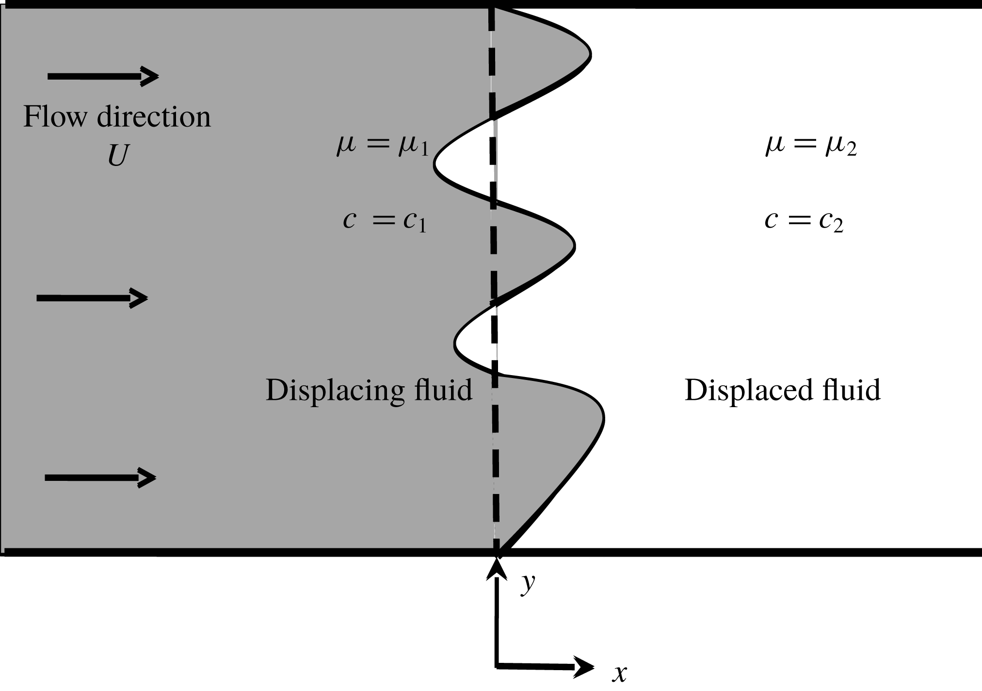
Schematic of the flow configuration with coordinate system. Initially the interface is located at
 $x=0$
shown as the dashed line.

Consider the miscible displacement flow in a porous media as shown in figure 1. The fluid of viscosity
 $\unicode[STIX]{x1D707}_{1}$
displaces a fluid of viscosity,
 $\unicode[STIX]{x1D707}_{2}$
, with a uniform velocity
 $U$
. The fluids are assumed to be Newtonian, non-reactive and neutrally buoyant, and the porous medium is homogeneous with a constant permeability and isotropic dispersion. Fluid flow and mass transport in the porous medium are governed by the equations for conservation of mass, conservation of momentum in the form of Darcy’s law and the volume-averaged mass balance equation in the form of a convection–diffusion equation which are given by
 $$\begin{eqnarray}\displaystyle & \displaystyle \unicode[STIX]{x1D735}\boldsymbol{\cdot }\boldsymbol{u}=0, & \displaystyle\end{eqnarray}$$
 $$\begin{eqnarray}\displaystyle & \displaystyle \unicode[STIX]{x1D735}p=-\unicode[STIX]{x1D707}\boldsymbol{u}, & \displaystyle\end{eqnarray}$$
 $$\begin{eqnarray}\displaystyle & \displaystyle \frac{\unicode[STIX]{x2202}c}{\unicode[STIX]{x2202}t}+\boldsymbol{u}\boldsymbol{\cdot }\unicode[STIX]{x1D735}c=D\unicode[STIX]{x1D6FB}^{2}c, & \displaystyle\end{eqnarray}$$
 $$\begin{eqnarray}\displaystyle & \displaystyle \unicode[STIX]{x1D707}=\unicode[STIX]{x1D707}(c), & \displaystyle\end{eqnarray}$$
where
 $\boldsymbol{u}=(u,v)$
is the two-dimensional Darcy velocity,
 $c$
is the solute concentration,
 $p$
is the fluid pressure,
 $\unicode[STIX]{x1D707}$
is the dynamic viscosity and
 $D$
is the isotropic dispersion coefficient taken throughout to be constant. At the initial time
 $t=0$
, the concentration and viscosity of the displacing fluid are
 $c_{1}$
and
 $\unicode[STIX]{x1D707}_{1}$
, respectively whereas the displaced fluid has concentration and viscosity as
 $c_{2}$
and
 $\unicode[STIX]{x1D707}_{2}$
, respectively.
In the present work, we have used Darcy’s law to describe the flow in a porous medium or equivalently Hele-Shaw flow within a thin gap approximation. In particular, equation (2.2) is obtained by averaging the parabolic velocity profile in between the parallel plates. The mathematical analysis of Darcy’s law in thin regions has been studied extensively, e.g. for averaging of creeping flow (Bayada & Chambat Reference Bayada and Chambat1986) and for averaging of Navier–Stokes systems (Nazarov Reference Nazarov1990). Validity of Darcy’s law, in continuum modelling of flows in porous media, implicitly assumed that the viscosity varies over the macroscopic scale and can be treated as constant on the micro-scale on which the permeability is computed. Similarly, Zick & Homsy (Reference Zick and Homsy1982) observed that the viscosity variation is slow relative to the grain size, so that the force is determined to a good approximation by a constant viscous stress. In addition Nagatsu & De Wit (Reference Nagatsu and De Wit2011) and Riolfo et al. (Reference Riolfo, Nagatsu, Iwata, Maes, Trevelyan and De Wit2012) successfully showed that the experimental findings agree meticulously with the numerical simulation of reaction-driven viscous fingering based on a Darcy’s law model.
In order to make the governing equations dimensionless, characteristic scales have to be introduced. We note that the set of equations (2.1)–(2.4) involves neither a characteristic time scale nor a length scale; so the equations are made dimensionless using diffusive scaling, i.e. we considered the characteristic length
 $D/U$
and time
 $D/U^{2}$
, where
 $D$
is the isotropic dispersion coefficient. Thus the non-dimensional form of the equations that govern the two-dimensional flow in a reference frame moving with constant injection velocity
 $U$
are described by (Manickam & Homsy Reference Manickam and Homsy1993)
 $$\begin{eqnarray}\displaystyle & \displaystyle \unicode[STIX]{x1D735}\boldsymbol{\cdot }\boldsymbol{u}=0, & \displaystyle\end{eqnarray}$$
 $$\begin{eqnarray}\displaystyle & \displaystyle \unicode[STIX]{x1D735}p=-\unicode[STIX]{x1D707}(c)(\boldsymbol{u}+\hat{i} ), & \displaystyle\end{eqnarray}$$
 $$\begin{eqnarray}\displaystyle & \displaystyle \frac{\unicode[STIX]{x2202}c}{\unicode[STIX]{x2202}t}+\boldsymbol{u}\boldsymbol{\cdot }\unicode[STIX]{x1D735}c=\unicode[STIX]{x1D6FB}^{2}c, & \displaystyle\end{eqnarray}$$
where velocity, concentration, viscosity and pressure are non-dimensionalized with
 $U$
,
 $(c-c_{1})/(c_{2}-c_{1})$
,
 $\unicode[STIX]{x1D707}_{1}$
, and
 $p/\unicode[STIX]{x1D707}_{1}D$
, respectively. Here
 $\hat{i}$
is the unit vector along the main flow direction, i.e. the
 $x$
direction.
The initial and boundary conditions associated with the coupled equations (2.5)–(2.7) are as follows (Nield & Bejan Reference Nield and Bejan1992).
Initial conditions:
 $$\begin{eqnarray}\displaystyle & \displaystyle \boldsymbol{u}(x,y,t=0)=(u,v)(x,y,t=0)=(0,0), & \displaystyle\end{eqnarray}$$
 $$\begin{eqnarray}\displaystyle & \displaystyle \text{and }\forall y,\quad c(x,y,t=0)=\left\{\begin{array}{@{}ll@{}}1,\quad & x<0\\ 0,\quad & x\geqslant 0.\end{array}\right. & \displaystyle\end{eqnarray}$$
Boundary conditions:
 $$\begin{eqnarray}\displaystyle \boldsymbol{u}=(0,0),\quad \frac{\unicode[STIX]{x2202}c}{\unicode[STIX]{x2202}x}\rightarrow 0,\quad |x|\rightarrow \infty ,\quad \text{streamwise direction}, & & \displaystyle\end{eqnarray}$$
 $$\begin{eqnarray}\displaystyle u=0,\quad \frac{\unicode[STIX]{x2202}v}{\unicode[STIX]{x2202}y}\rightarrow 0,\quad \frac{\unicode[STIX]{x2202}c}{\unicode[STIX]{x2202}y}\rightarrow 0,\quad |y|\rightarrow \infty ,\quad \text{spanwise direction}, & & \displaystyle\end{eqnarray}$$
where
 $u$
and
 $v$
are the axial and transverse components of the two-dimensional velocity
 $\boldsymbol{u}$
. Further, the coupled equations (2.5)–(2.7) admit the following transient base state,
 $$\begin{eqnarray}\displaystyle \boldsymbol{u}_{b}=(0,0),\quad c_{b}=\frac{1}{2}\left[1-\text{erf}\left(\frac{x}{2\sqrt{t}}\right)\right],\quad p_{b}(x,t)=-\!\int _{-\infty }^{x}\unicode[STIX]{x1D707}_{b}(s,t)\,\text{d}s,\qquad & & \displaystyle\end{eqnarray}$$
by solving the equations
 $$\begin{eqnarray}\displaystyle \frac{\unicode[STIX]{x2202}p_{b}}{\unicode[STIX]{x2202}x}=-\unicode[STIX]{x1D707}\quad \text{and}\quad \frac{\unicode[STIX]{x2202}c_{b}}{\unicode[STIX]{x2202}t}=\frac{\unicode[STIX]{x2202}^{2}c_{b}}{\unicode[STIX]{x2202}x^{2}}. & & \displaystyle\end{eqnarray}$$
Here
 $\text{erf}(\cdot )$
is the error function and the subscript
 $b$
stands for the base state.
2.1 Non-monotonic viscosity relationship
The exact nature of the relationship between the dynamic viscosity
 $\unicode[STIX]{x1D707}$
and concentration
 $c$
will depend on the particular combination of fluids under consideration (Pankiewitz & Meiburg Reference Pankiewitz and Meiburg1999; Haudin et al.
Reference Haudin, Callewaert, De Malsche and De Wit2016). It has been observed that there exists an alcohol–water pair for which viscosity
 $\unicode[STIX]{x1D707}(c)$
can achieve a maximum at some intermediate local concentration composition
 $c$
(Manickam & Homsy Reference Manickam and Homsy1993, Reference Manickam and Homsy1994; Schafroth et al.
Reference Schafroth, Goyal and Meiburg2007; Haudin et al.
Reference Haudin, Callewaert, De Malsche and De Wit2016). In other words, the flow develops a potentially unstable region followed downstream by a potentially stable region or vice versa. In this scenario, the stable region acts as a barrier to the growth of fingers, thereby providing a mechanism to control the VF. Hence, a fundamental understanding of the finger propagation in flows with non-monotonic viscosity profiles is essential to develop methodologies aimed at controlling the growth of viscous fingers. In order to understand the influence of non-monotonic viscosity profiles, we focus on the non-monotonic viscosity–concentration model proposed by Manickam & Homsy (Reference Manickam and Homsy1993).
In order to allow comparisons with earlier studies of rectilinear displacements, we employ the non-monotonic class of viscosity–concentration profiles used by Manickam & Homsy (Reference Manickam and Homsy1993, Reference Manickam and Homsy1994) and Pankiewitz & Meiburg (Reference Pankiewitz and Meiburg1999). The viscosity–concentration profiles are sine functions modified through a sequence of transformations which is well-suited to the non-monotonic profiles of alcohol mixtures (Weast Reference Weast1990) and is given by the expressions
 $$\begin{eqnarray}\displaystyle & \displaystyle \unicode[STIX]{x1D707}(c)=\unicode[STIX]{x1D707}_{m}\sin (\unicode[STIX]{x1D701}), & \displaystyle\end{eqnarray}$$
 $$\begin{eqnarray}\displaystyle & \displaystyle \unicode[STIX]{x1D701}=\unicode[STIX]{x1D701}_{0}(1-\unicode[STIX]{x1D702})+\unicode[STIX]{x1D701}_{1}\unicode[STIX]{x1D702}, & \displaystyle\end{eqnarray}$$
 $$\begin{eqnarray}\displaystyle & \displaystyle \unicode[STIX]{x1D702}=\frac{(1+a)c}{1+ac}, & \displaystyle\end{eqnarray}$$
where
 $$\begin{eqnarray}\left.\begin{array}{@{}c@{}}\displaystyle \unicode[STIX]{x1D701}_{0}=\arcsin (\unicode[STIX]{x1D6FC}/\unicode[STIX]{x1D707}_{m}),\\ \displaystyle \unicode[STIX]{x1D701}_{1}=\unicode[STIX]{x03C0}-\arcsin (1/\unicode[STIX]{x1D707}_{m}),\\ \displaystyle a=\frac{c_{m}-\unicode[STIX]{x1D702}_{m}}{c_{m}(\unicode[STIX]{x1D702}_{m}-1)},\\ \displaystyle \unicode[STIX]{x1D702}_{m}=\frac{\unicode[STIX]{x03C0}/2-\unicode[STIX]{x1D701}_{0}}{\unicode[STIX]{x1D701}_{1}-\unicode[STIX]{x1D701}_{0}},\text{ and }\unicode[STIX]{x1D6FC}=\unicode[STIX]{x1D707}_{2}/\unicode[STIX]{x1D707}_{1}.\end{array}\right\}\end{eqnarray}$$
The transformations are defined in such a way that the endpoint values are
 $\unicode[STIX]{x1D707}(0)=\unicode[STIX]{x1D6FC}$
,
 $\unicode[STIX]{x1D707}(1)=1$
and they attain a maximum value
 $\unicode[STIX]{x1D707}_{m}$
at
 $c=c_{m}$
.
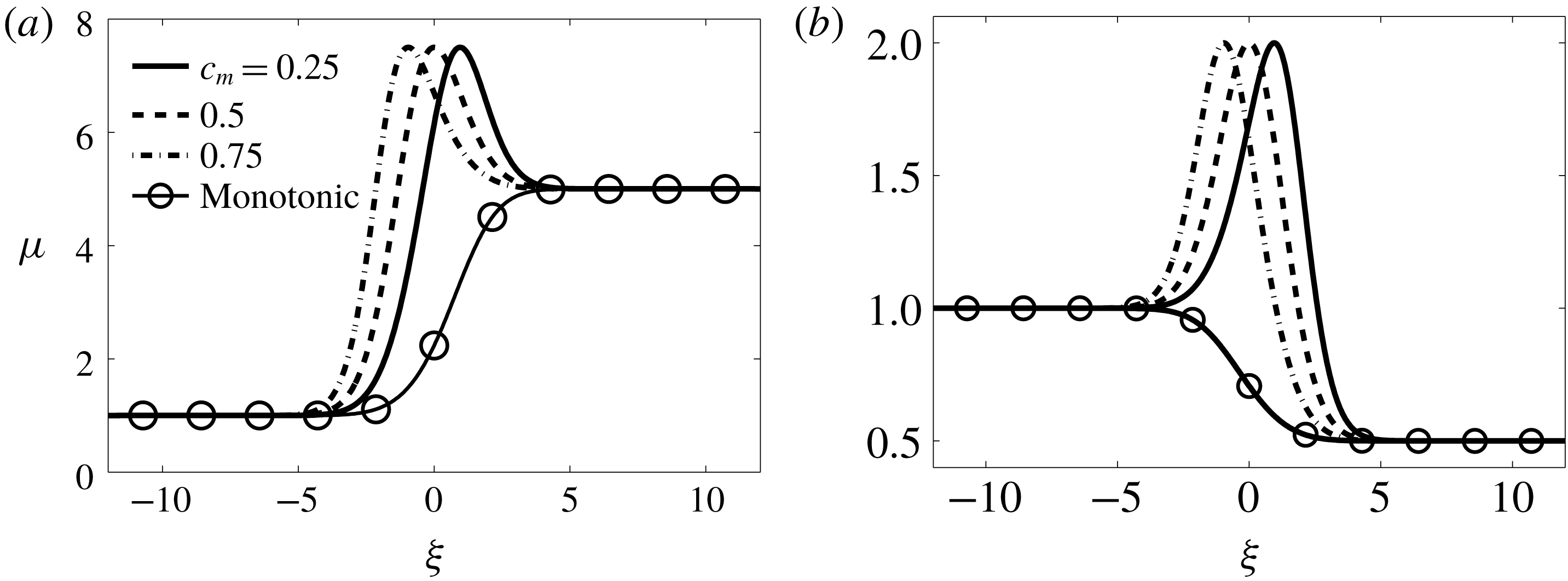
Spatial variation of the viscosity relation (2.14) in a self-similar coordinate
 $\unicode[STIX]{x1D709}=x/\sqrt{t}$
for (a)
 $\unicode[STIX]{x1D6FC}=5,\unicode[STIX]{x1D707}_{m}=7.5$
and (b)
 $\unicode[STIX]{x1D6FC}=0.5,\unicode[STIX]{x1D707}_{m}=2$
. The monotonic viscosity is
 $\unicode[STIX]{x1D707}(c)=\exp (\ln (\unicode[STIX]{x1D6FC})(1-c))$
.

The non-monotonic profile of dynamic viscosity is characterized by a family of curves described by three parameters, namely,
 $\unicode[STIX]{x1D6FC},c_{m}$
and
 $\unicode[STIX]{x1D707}_{m}$
. The parameter
 $\unicode[STIX]{x1D6FC}$
is the ratio of the endpoint viscosities, i.e.
 $\unicode[STIX]{x1D6FC}=\unicode[STIX]{x1D707}_{2}/\unicode[STIX]{x1D707}_{1}$
, the traditional measure of stability in viscous fingering. In particular, for
 $\unicode[STIX]{x1D6FC}<1$
the flow is said to have a favourable viscosity contrast, and when
 $\unicode[STIX]{x1D6FC}>1$
, the flow is said to have an unfavourable viscosity contrast. Figure 2(a,b) demonstrates the spatial variation of
 $\unicode[STIX]{x1D707}(c)$
for
 $\unicode[STIX]{x1D6FC}=5,\unicode[STIX]{x1D707}_{m}=7.5$
and
 $\unicode[STIX]{x1D6FC}=0.5,\unicode[STIX]{x1D707}_{m}=2$
, for different values of
 $c_{m}$
. It can be noted that for
 $c_{m}>0.5$
,
 $\unicode[STIX]{x1D707}_{m}$
is located closer to the displacing fluid, while it is near to the displaced fluid if
 $c_{m}<0.5$
. Manickam & Homsy (Reference Manickam and Homsy1993) showed that the stability criterion for non-monotonic profiles (2.14) is determined by a parameter,
 $\unicode[STIX]{x1D712}$
, that relates the endpoint slopes of the viscosity profile which is defined as
 $$\begin{eqnarray}\displaystyle \unicode[STIX]{x1D712}=-\left(\frac{\left.\displaystyle \frac{\text{d}\unicode[STIX]{x1D707}}{\text{d}c}\right|_{c=0}+\left.\displaystyle \frac{\text{d}\unicode[STIX]{x1D707}}{\text{d}c}\right|_{c=1}}{\unicode[STIX]{x1D6FC}+1}\right). & & \displaystyle\end{eqnarray}$$
In particular, the system is stable if
 $\unicode[STIX]{x1D712}<0$
, otherwise it is unstable. For the monotonic case, i.e.
 $\unicode[STIX]{x1D707}(c)=\exp (R(1-c)),R=\ln (\unicode[STIX]{x1D6FC})$
, we have
 $\unicode[STIX]{x1D712}=R$
. In contrast, in the non-monotonic case the sign of
 $\unicode[STIX]{x1D712}$
depends on the magnitude of the gradient at the endpoints. Thus, in the non-monotonic case, the stability depends not on the endpoint viscosities but on the derivative of the viscosity with respect to concentration at the endpoints.
2.2 Linear stability analysis
In order to carry out the linear stability analysis, we introduce an infinitesimal perturbation to the base state, equation (2.12). Then, we linearize the equations (2.5)–(2.7) about the base state (2.12) and eliminate the pressure and transverse velocity disturbances by taking the curl of Darcy’s law and utilizing the continuity equation. The final form of the linearized perturbation equations is given by (Manickam & Homsy Reference Manickam and Homsy1993)
 $$\begin{eqnarray}\displaystyle M_{1}u^{\prime }=M_{2}c^{\prime },\quad \frac{\unicode[STIX]{x2202}c^{\prime }}{\unicode[STIX]{x2202}t}=M_{3}c^{\prime }+M_{4}u^{\prime }, & & \displaystyle\end{eqnarray}$$
where
 $c^{\prime }$
and
 $u^{\prime }$
denote the perturbation quantities representing the concentration and the axial velocity component, respectively, and
 $$\begin{eqnarray}\left.\begin{array}{@{}c@{}}\displaystyle M_{1}={\mathcal{D}}_{x}^{2}+\frac{1}{\unicode[STIX]{x1D707}_{b}}({\mathcal{D}}_{x}c_{b}){\mathcal{D}}_{x}+\unicode[STIX]{x1D707}_{b}{\mathcal{D}}_{y}^{2},\quad M_{2}=-R(\unicode[STIX]{x1D707}_{b}){\mathcal{D}}_{y}^{2},\\ \displaystyle M_{3}={\mathcal{D}}_{x}^{2}+{\mathcal{D}}_{y}^{2},\quad M_{4}=-{\mathcal{D}}_{x}c_{b},\end{array}\right\}\end{eqnarray}$$
 ${\mathcal{D}}_{x}^{n}=\unicode[STIX]{x2202}^{n}/\unicode[STIX]{x2202}x^{n},{\mathcal{D}}_{y}^{n}=\unicode[STIX]{x2202}^{n}/\unicode[STIX]{x2202}y^{n},n=1,2$
. Since the coefficients of the above equations are independent of
 $y$
, the disturbances are decomposed in terms of Fourier components in the
 $y$
direction,
 $$\begin{eqnarray}\displaystyle [c^{\prime },u^{\prime }](x,y,t)=[\unicode[STIX]{x1D719}_{c},\unicode[STIX]{x1D719}_{u}](x,t)\text{e}^{\text{i}ky},\quad \text{i}=\sqrt{-1}, & & \displaystyle\end{eqnarray}$$
where
 $k$
is the non-dimensional wavenumber. Using (2.21), the operators in (2.20) can be recast as
 $$\begin{eqnarray}\left.\begin{array}{@{}c@{}}\displaystyle M_{1}={\mathcal{D}}_{x}^{2}+\frac{1}{\unicode[STIX]{x1D707}_{b}}({\mathcal{D}}_{x}c_{b}){\mathcal{D}}_{x}-k^{2}\unicode[STIX]{x1D707}_{b}\unicode[STIX]{x1D644},\quad M_{2}=k^{2}R(\unicode[STIX]{x1D707}_{b})\unicode[STIX]{x1D644},\\ \displaystyle M_{3}={\mathcal{D}}_{x}^{2}-k^{2}\unicode[STIX]{x1D644},\quad M_{4}=-{\mathcal{D}}_{x}c_{b},\end{array}\right\}\end{eqnarray}$$
where
 $\unicode[STIX]{x1D644}$
is the identity operator and
 $R(\unicode[STIX]{x1D707}_{b})$
is a viscosity-related parameter given by
 $$\begin{eqnarray}\displaystyle R(\unicode[STIX]{x1D707}_{b})=\frac{1}{\unicode[STIX]{x1D707}_{b}}\frac{\text{d}\unicode[STIX]{x1D707}_{b}}{\text{d}c_{b}}=\frac{(1+a)(\unicode[STIX]{x1D701}_{1}-\unicode[STIX]{x1D701}_{0})}{(1+ac_{b})^{2}}\cot (\unicode[STIX]{x1D701}). & & \displaystyle\end{eqnarray}$$
Here,
 $\unicode[STIX]{x1D707}_{b}$
and
 $c_{b}$
are the viscosity and concentration base states, respectively. It is easily verifiable that for monotonic viscosity–concentration profiles,
 $R(\unicode[STIX]{x1D707}_{b})=R=\ln (\unicode[STIX]{x1D6FC})$
, the log-mobility ratio. Now, the linearized (2.19) can be recast as an initial boundary value problem,
 $$\begin{eqnarray}\displaystyle \frac{\unicode[STIX]{x2202}\unicode[STIX]{x1D719}_{c}}{\unicode[STIX]{x2202}t}=\widetilde{{\mathcal{L}}}\unicode[STIX]{x1D719}_{c}, & & \displaystyle\end{eqnarray}$$
where
 $\widetilde{{\mathcal{L}}}=M_{3}+M_{4}M_{1}^{-1}M_{2}$
, and
 $M_{i}$
values are as in (2.22). The associated boundary conditions are
 $(\unicode[STIX]{x1D719}_{c},\unicode[STIX]{x1D719}_{u})\rightarrow 0,$
as
 $x\rightarrow \pm \infty$
and a random initial condition. Manickam & Homsy (Reference Manickam and Homsy1993, Reference Manickam and Homsy1994) analyse the stability of (2.24) by using a quasi-steady-state approximation (QSSA) and compare linear stability results with nonlinear simulations. They have shown that the validity of the QSSA is questionable at short times where the base state changes rapidly. A fundamental problem with such an approach is that the concentration eigenfunctions span the entire spatial domain, i.e. the eigenfunctions of the operator
 ${\mathcal{D}}_{x}^{2}=\unicode[STIX]{x2202}^{2}/\unicode[STIX]{x2202}x^{2},x\in (-\infty ,\infty )$
are global modes. Hence, they do not provide an appropriate basis for streamwise perturbations (Ben et al.
Reference Ben, Demekhin and Chang2002). As the present problem can have a small onset time (
 $t\approx O(1)$
) for instability, the QSSA as such is ill-suited to the task of resolving the early-time behaviour. To overcome this difficulty, Kim & Choi (Reference Kim and Choi2011) uses the self-similar property of the base state, i.e. they transform the
 $(x,t)$
coordinate to a self-similar coordinate
 $(\unicode[STIX]{x1D709},t)$
,
 $\unicode[STIX]{x1D709}=x/\sqrt{t}$
such that the base state, equation (2.12), becomes
 $c_{b}(\unicode[STIX]{x1D709})=(1/2)[1-\text{erf}(\unicode[STIX]{x1D709}/2)]$
. In the self-similar coordinate
 $(\unicode[STIX]{x1D709},t)$
, the streamwise operator,
 $$\begin{eqnarray}\boldsymbol{T}=\frac{\unicode[STIX]{x2202}^{2}}{\unicode[STIX]{x2202}\unicode[STIX]{x1D709}^{2}}+\frac{\unicode[STIX]{x1D709}}{2}\frac{\unicode[STIX]{x2202}}{\unicode[STIX]{x2202}\unicode[STIX]{x1D709}},\end{eqnarray}$$
satisfies the eigenvalue problem
 $$\begin{eqnarray}\displaystyle \boldsymbol{T}e_{n}(\unicode[STIX]{x1D709})=\unicode[STIX]{x1D706}_{n}e_{n}(\unicode[STIX]{x1D709})=\unicode[STIX]{x1D706}_{n}a_{n}{\mathcal{H}}_{n}(\unicode[STIX]{x1D709}/2)\exp (-\unicode[STIX]{x1D709}^{2}/4),\quad n=0,1,2,\ldots , & & \displaystyle\end{eqnarray}$$
where
 ${\mathcal{H}}_{n}(\unicode[STIX]{x1D709})$
is the
 $n$
th Hermite polynomial,
 $a_{n}$
are positive constants and
 $\unicode[STIX]{x1D706}_{n}=-(n+1)/2$
. The Hermite function based eigenfunctions, being localized around the base state, provide an optimal basis for streamwise perturbations. This suggests that the numerical simulation of the miscible viscous fingering dynamics in an unbounded domain is best done in the
 $(\unicode[STIX]{x1D709},t)$
coordinates. For this reason we have investigated the stability analysis of miscible viscous fingering in
 $(\unicode[STIX]{x1D709},t)$
coordinates. On rewriting (2.24) in transformed coordinates
 $(\unicode[STIX]{x1D709},t)$
, we have
 $$\begin{eqnarray}\displaystyle \frac{\unicode[STIX]{x2202}\unicode[STIX]{x1D719}_{c}}{\unicode[STIX]{x2202}t}={\mathcal{L}}(t)\unicode[STIX]{x1D719}_{c}, & & \displaystyle\end{eqnarray}$$
where
 ${\mathcal{L}}(t)=T_{3}+T_{4}T_{1}^{-1}T_{2}$
, and
 $T_{i}$
values are as follows:
 $$\begin{eqnarray}\left.\begin{array}{@{}c@{}}\displaystyle T_{1}={\mathcal{D}}^{\prime 2}+\frac{1}{\unicode[STIX]{x1D707}_{b}}\frac{\text{d}\unicode[STIX]{x1D707}_{b}}{\text{d}\unicode[STIX]{x1D709}}{\mathcal{D}}^{\prime }-k^{2}t\unicode[STIX]{x1D644},\quad T_{2}=k^{2}tR(\unicode[STIX]{x1D707}_{b})\unicode[STIX]{x1D644},\\ \displaystyle T_{3}=\frac{1}{t}{\mathcal{D}}^{\prime 2}+\frac{\unicode[STIX]{x1D709}}{2t}{\mathcal{D}}^{\prime }-k^{2}\unicode[STIX]{x1D644},\quad T_{4}=-\frac{1}{\sqrt{t}}\frac{\text{d}c_{b}}{\text{d}\unicode[STIX]{x1D709}}\unicode[STIX]{x1D644},\end{array}\right\}\end{eqnarray}$$
 ${\mathcal{D}}^{\prime n}=\unicode[STIX]{x2202}^{n}/\unicode[STIX]{x2202}\unicode[STIX]{x1D709}^{n},n=1,2$
and
 $R(\unicode[STIX]{x1D707}_{b})$
as in (2.23). Even though the two sets of equations (2.24) and (2.27) are mathematically equivalent, there is one restriction. It is observed that the transformation to the self-similar coordinates
 $(x,t)\rightarrow (\unicode[STIX]{x1D709},t)$
is singular at
 $t=0$
. Hence, we must restrict our evolution away from this singular limit
 $t=0$
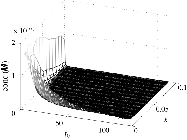
. The omission of this singular limit is not practically important. Further, we have presented the relationship between the onset time and energy of the perturbations that is obtained from both the coordinates in appendix B.
2.3 Non-modal analysis
As the linear stability operator,
 ${\mathcal{L}}(t)$
, in (2.27) is non-autonomous, we have employed the non-modal analysis (NMA) described by Schmid (Reference Schmid2007). We first discretize the linearized disturbance system, equation (2.27), to get an initial value problem (IVP):
 $$\begin{eqnarray}\displaystyle \frac{\text{d}\unicode[STIX]{x1D719}_{c}}{\text{d}t}={\mathcal{L}}(t)\unicode[STIX]{x1D719}_{c}. & & \displaystyle\end{eqnarray}$$
For a chosen time interval
 $[t_{p},t_{f}]$
, let
 $\unicode[STIX]{x1D6F7}(t_{p};t_{f})$
be a formal solution of (2.29), where
 $\unicode[STIX]{x1D719}_{c}(t_{f})=\unicode[STIX]{x1D6F7}(t_{p};t_{f})\unicode[STIX]{x1D719}_{c}(t_{p})$
,
 $\unicode[STIX]{x1D719}_{c}(t_{p})$
being an arbitrary initial condition. Substitute this value of
 $\unicode[STIX]{x1D719}_{c}(t_{f})$
in (2.29) to get a matrix-valued IVP,
 $$\begin{eqnarray}\frac{\text{d}}{\text{d}t}\unicode[STIX]{x1D6F7}(t_{p};t_{f})={\mathcal{L}}(t_{f})\unicode[STIX]{x1D6F7}(t_{p};t_{f}),\end{eqnarray}$$
with initial condition
 $\unicode[STIX]{x1D6F7}(t_{p};t_{p})=\unicode[STIX]{x1D644}$
, where
 $\unicode[STIX]{x1D644}$
is the identity matrix. The operator
 $\unicode[STIX]{x1D6F7}(t_{p};t_{f})$
propagating the information from initial perturbation time
 $t_{p}$
(time at which the perturbation is introduced to the base state) to final time
 $t_{f}$
is known as the propagator operator. It can be noted that the existence and uniqueness of the solution to (2.29) can be established under the hypothesis that the map
 $t\rightarrow {\mathcal{L}}(t)$
is continuous from
 $\mathbb{R}^{+}$
to the set of
 $n\times n$
matrix over real numbers
 $\mathbb{R}$
(Vidyasagar Reference Vidyasagar2002). Further, assuming that
 $\unicode[STIX]{x1D719}_{c}$
is square integrable over
 $\mathbb{R}$
, we wish to find the maximum perturbation energy gain, that is,
 $$\begin{eqnarray}\displaystyle G(t_{f}) & = & \displaystyle G(t_{f},k,Pe,R,\unicode[STIX]{x1D6FF}):=\max _{\unicode[STIX]{x1D719}_{c}(t_{p})}\frac{E_{\unicode[STIX]{x1D719}_{c}}(t_{f})}{E_{\unicode[STIX]{x1D719}_{c}}(t_{p})}\nonumber\\ \displaystyle & = & \displaystyle \max _{\unicode[STIX]{x1D719}_{c}(t_{p})}\Vert \unicode[STIX]{x1D6F7}(t_{p};t_{f})\unicode[STIX]{x1D719}_{c}(t_{p})\Vert _{2}=\Vert \unicode[STIX]{x1D6F7}(t_{p};t_{f})\Vert =\sup _{j}s_{j}(t_{f}),\end{eqnarray}$$
where
 $s_{j}$
values are the singular values of
 $\unicode[STIX]{x1D6F7}(t_{p};t_{f})$
, in other words, the eigenvalues of the self-adjoint matrix
 $\unicode[STIX]{x1D6F7}^{\ast }(t_{p};t_{f})\unicode[STIX]{x1D6F7}(t_{p};t_{f})$
can be found by singular value decomposition (SVD) of
 $\unicode[STIX]{x1D6F7}(t_{p};t_{f})$
. Here
 $E_{g}(t_{f}):=\Vert g(t_{f})\Vert _{2}^{2}=\int _{-\infty }^{\infty }|g(w,t_{f})|^{2}\,\text{d}w$
.
2.3.1 Numerical solution of the stability problem
In the stability (2.27), we have used a central finite difference scheme with uniform grids for all spatial derivatives and the fourth-order Runge–Kutta method for time integration. The advantage of the finite difference technique is that we can study the complete spectrum of the eigenvalues. The appropriate boundary conditions for all disturbances is that they must go to zero far from the front. Mathematically, this implies the appropriate eigenfunctions for the instability are localized and must be zero away from the interface. It has been observed from the standard spectral theory for an unbounded domain that due to this far-field boundary condition for disturbances, we only need to deal with the discrete eigenspectrum, instead of the essential modes whose eigenfunctions do not decay at the infinities of the governing operator
 ${\mathcal{L}}$
(Pego & Weinstein Reference Pego and Weinstein1994; Chang, Demekhin & Kalaidin Reference Chang, Demekhin and Kalaidin1998). This fact is also verified by Manickam & Homsy (Reference Manickam and Homsy1993). In our analysis, the infinite streamwise domain is truncated into a finite computational domain such that it can fully capture all the decaying discrete eigenfunctions. In order to check the validity of the results, the code was tested for several domain sizes and spatial step sizes. The results were reported if the obtained eigenvalues and eigenvectors are independent of domain and spatial step size. It is observed that the discrete eigenvalues associated with the velocity perturbations are sensitive to the width of the domain. We have performed numerical simulations by taking step size
 $h=0.1,0.15$
and
 $0.2$
. The relative error between the singular vectors has been calculated corresponding to all three simulations and it is found that the maximum relative error is of order
 $O(10^{-2})$
. The error has been calculated in terms of the standard Euclidean norm in
 $\mathbb{R}^{n}$
, defined as
 $\Vert \cdot \Vert ^{2}=\sum _{j=1}^{n}(\cdot )^{2}$
. Hence, for all simulations the spatial step size is taken to be
 $0.2$
with the computational domain
 $[-110,90]$
. Figure 5 shows that this domain length is good enough for our analysis. Further, the solution procedure has been validated by comparing with the linear stability results of Hota et al. (Reference Hota, Pramanik and Mishra2015a
) for Arrhenius type viscosity–concentration profiles.
3 Results and discussion
In order to understand the fundamental features and onset of instability in miscible displacements with non-monotonic viscosity profiles, we have studied two different cases, namely
 $\unicode[STIX]{x1D6FC}$
less than
 $1$
and greater than
 $1$
. Using NMA, we have shown that the singular vectors carry the information about coherent optimal perturbation structures and their temporal evolution. We validate our numerical findings by comparing with nonlinear simulations (NLS) performed using the Fourier pseudo-spectral method. Further, our results are in contrast to the existing linear stability analyses (Manickam & Homsy Reference Manickam and Homsy1993; Kim & Choi Reference Kim and Choi2011).
3.1 Stability analysis for unfavourable endpoint viscosity contrast
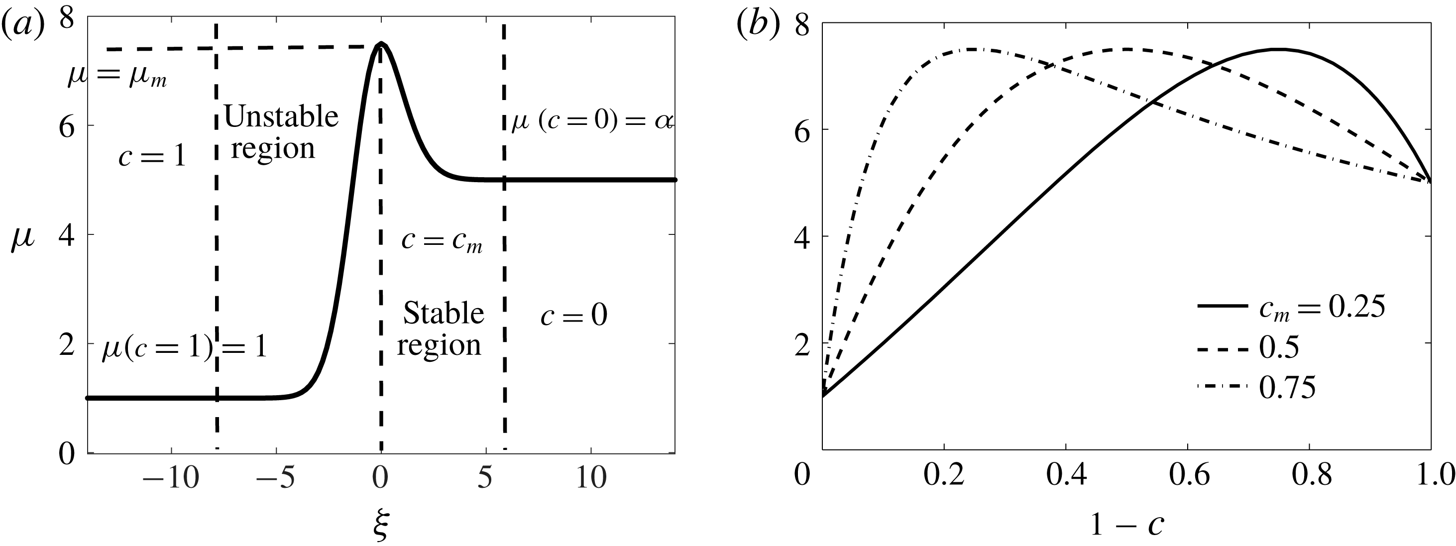
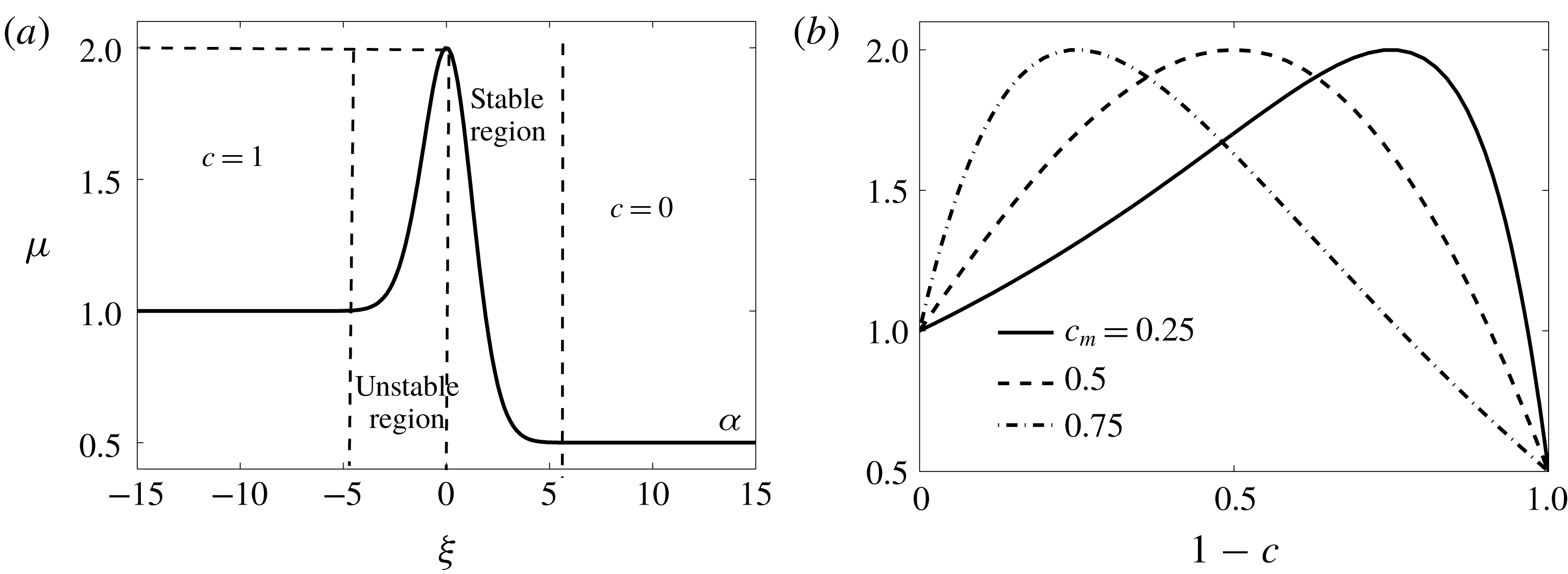
(a) Schematic of the spatial variation of viscosity for a diffused concentration profile and
 $\unicode[STIX]{x1D6FC}>1$
. (b) Viscosity profiles for
 $\unicode[STIX]{x1D6FC}=5,\unicode[STIX]{x1D707}_{m}=7.5$
and various values of
 $c_{m}$
. As
 $c_{m}$
increases, the viscosity gradient in the unstable region steepens.

In this case, we have
 $\unicode[STIX]{x1D6FC}>1$
, equivalently,
 $\unicode[STIX]{x1D707}_{1}<\unicode[STIX]{x1D707}_{2}$
. The spatial variation of the viscosity profile and the corresponding variation with concentration is given in figure 3(a,b), respectively. From figure 3 there develops a potentially unstable region, where the viscosity increases in the flow direction, followed in the downstream direction by a potentially stable region, where the viscosity decreases in the flow direction. In order to compare our results with the existing literature, we choose the following parameters:
 $\unicode[STIX]{x1D6FC}=5,\unicode[STIX]{x1D707}_{m}=7.5$
and
 $c_{m}=0.25,0.5$
and
 $0.75$
. With this configuration, the viscosity ratio within the unstable zone grows
 $7.5$
times, while it decreases moderately by a factor
 $7.5/5=1.5$
within the stable zone.
3.1.1 Optimal amplification
The optimal amplification,
 $G(t)$
, is the maximum possible energy that a perturbation can have, incorporating all possible initial conditions. From
 $G(t)$
, the onset of instability can be obtained as follows:
 $$\begin{eqnarray}\displaystyle t_{on}=\min \left\{t>0:\frac{\text{d}G(t)}{\text{d}t}=0\right\}. & & \displaystyle\end{eqnarray}$$
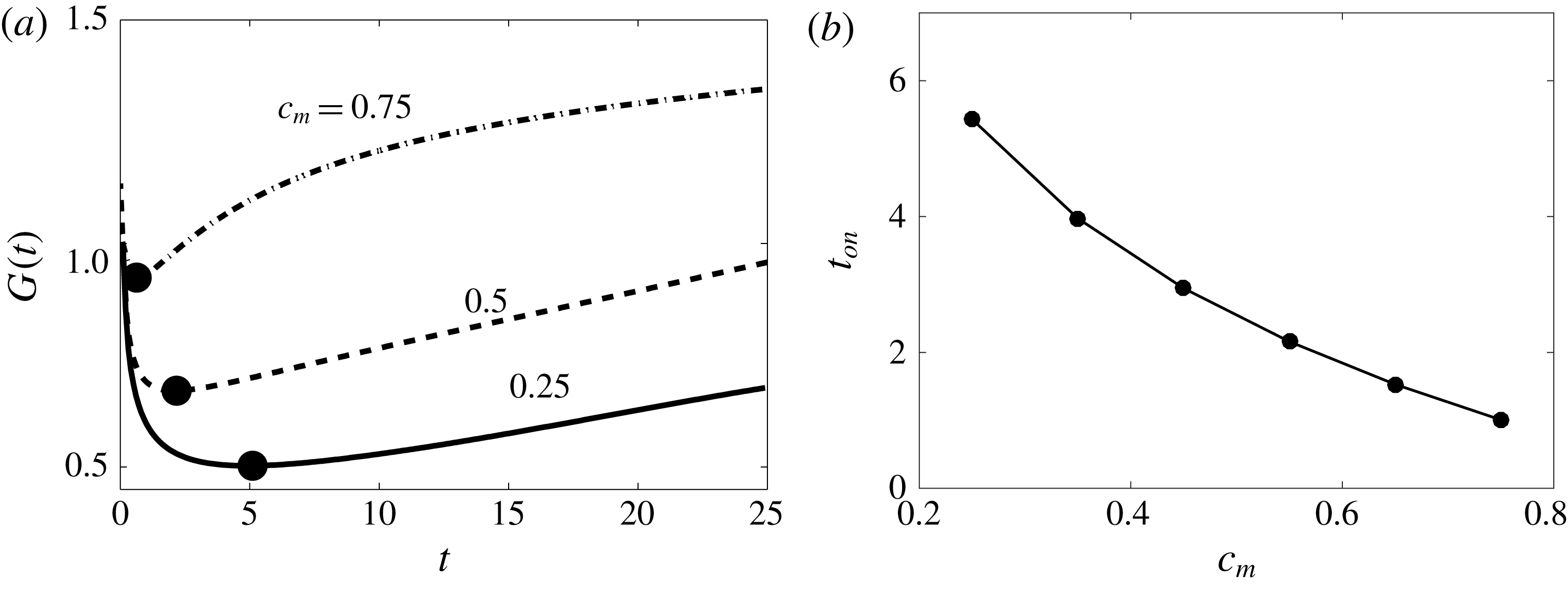
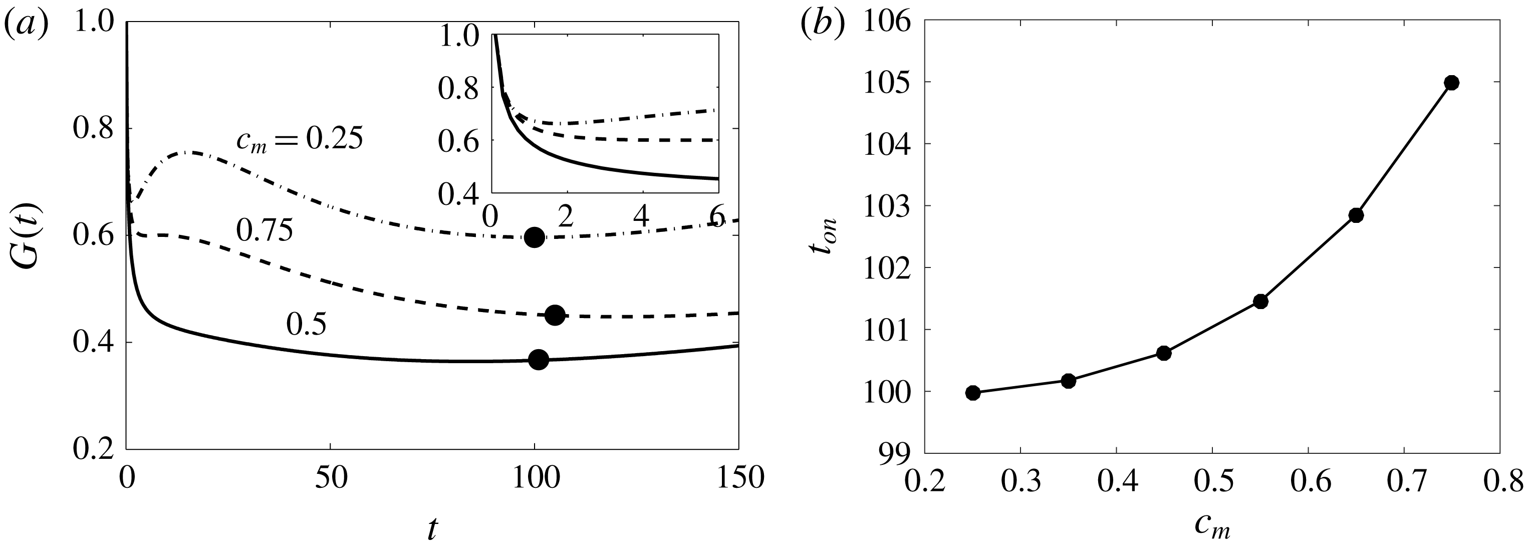
Figure 4(a) shows the optimal amplification,
 $G(t)$
(see (2.31)), for
 $\unicode[STIX]{x1D6FC}=5$
and
 $\unicode[STIX]{x1D707}_{m}=7.5$
and initial perturbation time
 $t_{p}=0.01$
. The initial perturbation time
 $t_{p}$
is chosen to be at least one order of magnitude smaller than the onset of instability,
 $t_{on}$
. We have shown in figure 4(b) that the onset times,
 $t_{on}$
, for
 $c_{m}=0.25,0.5$
and
 $0.75$
are found approximately to be
 $5.11,2.17$
and
 $0.63$
, respectively. In other words, we have found that for the parameters considered,
 $t_{on}$
is a decreasing function of
 $c_{m}$
. Further, the energy is most amplified for
 $c_{m}=0.75$
in comparison to
 $c_{m}=0.25$
and
 $0.5$
, which is in contrast to the findings of Manickam & Homsy (Reference Manickam and Homsy1993) and Kim & Choi (Reference Kim and Choi2011). These authors have shown that the instabilities set in the unstable region and propagate downstream into the stable barrier. Figure 3(a) illustrates that the concentration
 $c_{m}$
, at which the viscosity reaches a maximum, determines the length of the stable zone. Further, the larger the value of
 $c_{m}$
, the longer the stable zone and consequently its effectiveness in stunting the downstream propagation of the viscous fingers.
(a) Optimal amplification,
 $G(t)$
, for
 $\unicode[STIX]{x1D6FC}=5$
and
 $\unicode[STIX]{x1D707}_{m}=7.5$
for three different values of
 $c_{m}$
. The black dots (●) denote the onset of instability,
 $t_{on}$
. (b) Onset time,
 $t_{on}$
, is monotonically decreasing with increase in
 $c_{m}$
.

The unstable and stable interval for
 $(\unicode[STIX]{x1D6FC},\unicode[STIX]{x1D707}_{m})=(5,7.5)$
and
 $(0.5,2)$
(see figures 3
a and 7
a). The initial unperturbed interface is located at
 $\unicode[STIX]{x1D709}=0$
. In each case the left-hand endpoints are obtained when the value of
 $\unicode[STIX]{x1D707}$
is equal to
 $\unicode[STIX]{x1D707}(c=1)=1$
, and similarly the right-hand endpoints are obtained when the value is equal to
 $\unicode[STIX]{x1D707}(c=0)=\unicode[STIX]{x1D6FC}$
, with an absolute error of order
 $O(10^{-12})$
. It is evident that the stable region is increasing with an increase in the value of
 $c_{m}$
.

From table 1 and figure 3(b), it can be observed that although with the increase in
 $c_{m}$
one has a larger stable zone, the corresponding viscosity gradient is larger. In this light, the present contrasting results from NMA can be explained from the structure of the viscosity profiles. For
 $\unicode[STIX]{x1D6FC}=5,\unicode[STIX]{x1D707}_{m}=7.5$
, figure 3(b) depicts that as
 $c_{m}$
increases the resident fluid experiences an increase in viscosity. This enhances the energy of the perturbations and thus results in a early onset of instability. Note that the values of
 $\unicode[STIX]{x1D712}$
(as defined in (2.18)) for
 $c_{m}=0.25,0.5$
and
 $0.75$
are
 $-2.12,3.58$
and
 $14.05$
, respectively. This implies that there is a strong influence of the concentration gradient with respect to concentration in the non-monotonic viscosity profiles. Hence, it is shown that the endpoint viscosity gradient, along with the unfavourable endpoint viscosity contrast, have a substantial effect on the growth rate. The NMA findings are also supported by the findings of Wang (Reference Wang2014) on the radial miscible flow in a Hele-Shaw cell. Wang (Reference Wang2014) found that the time evolution of the interfacial length (which is a global measurement of the onset of fingering) suggests that for an unfavourable endpoint viscosity a higher value of
 $c_{m}$
leads to a more unstable interface at early times.
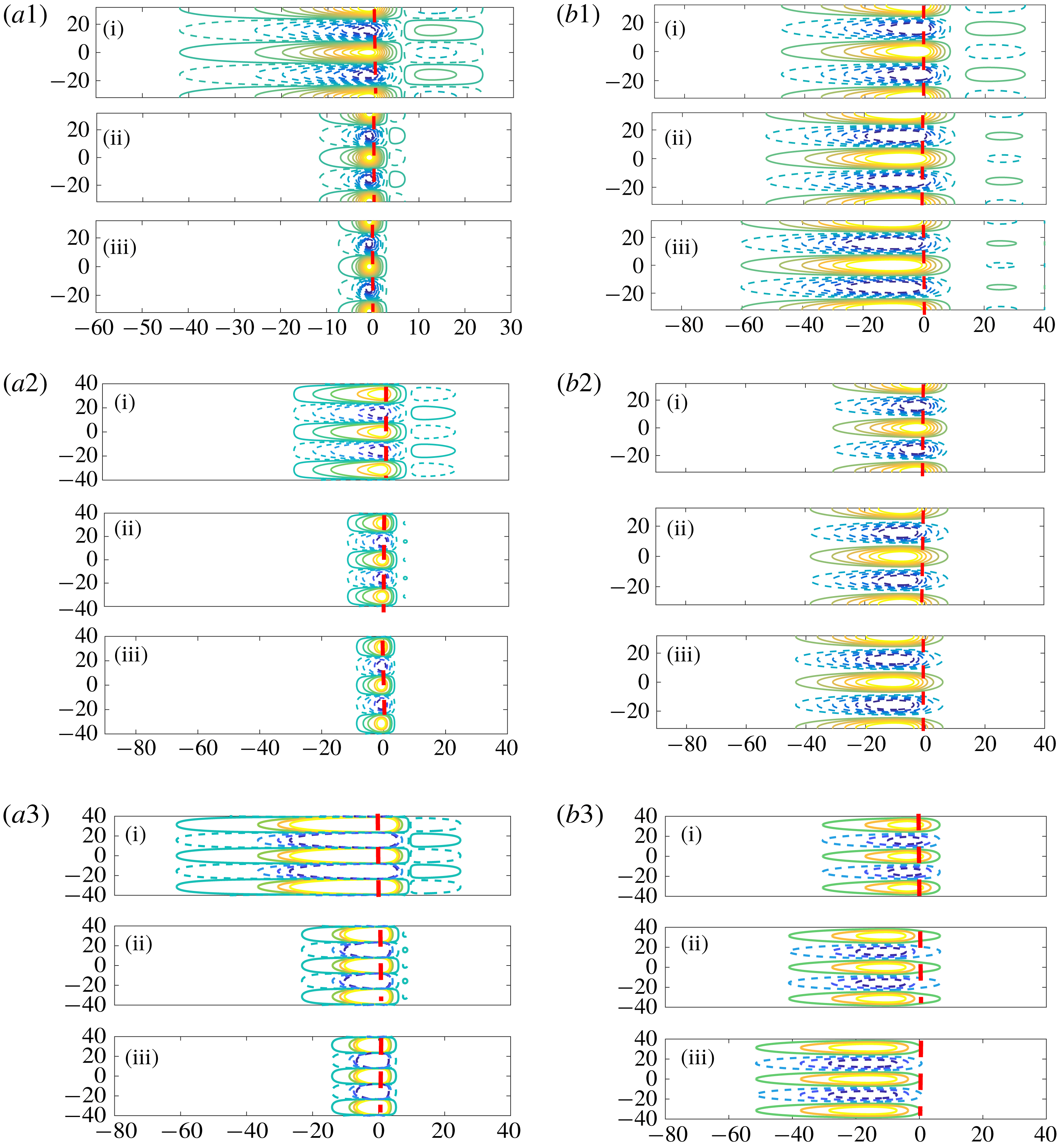
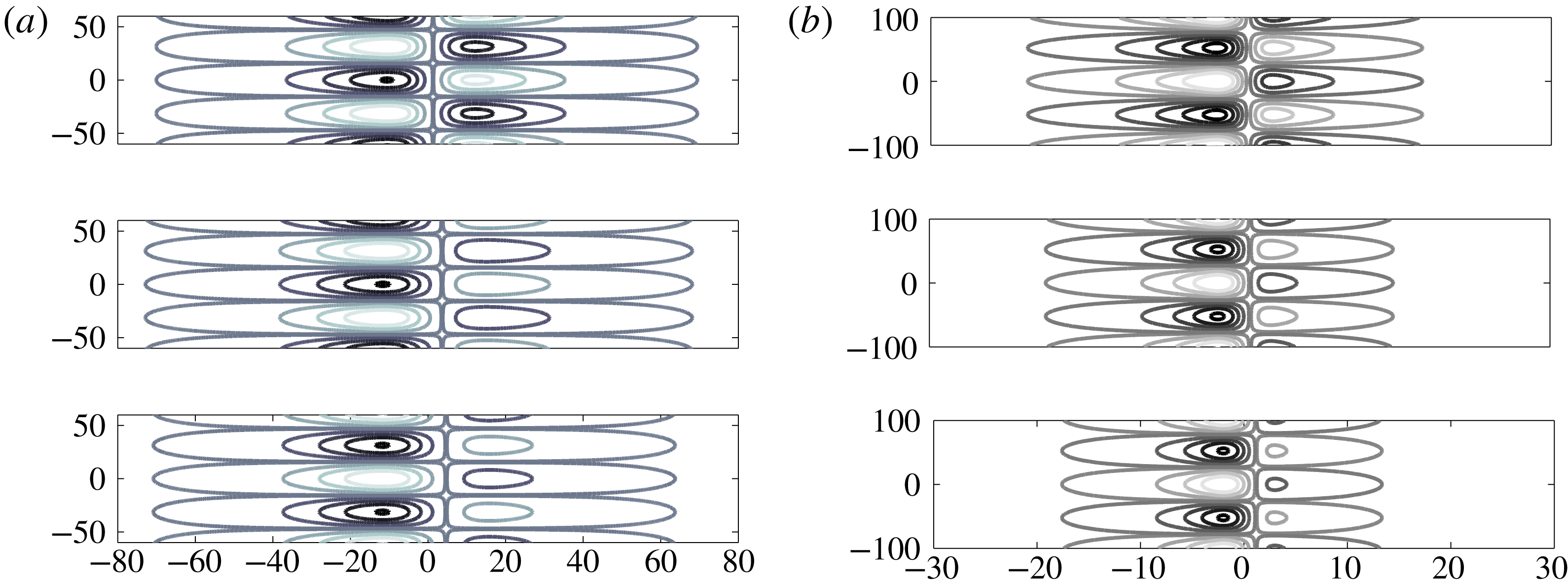
For
 $\unicode[STIX]{x1D6FC}=5,\unicode[STIX]{x1D707}_{m}=7.5,k=0.2$
, (a1–a3) the optimal initial perturbations,
 $c_{p}^{\prime }=V_{opt}\cos (ky)$
, and (b1–b3) the corresponding evolved state,
 $c^{\prime }=U_{opt}\cos (ky)$
. From top to bottom
 $c_{m}=0.25,0.5$
and
 $0.75$
. Here the time integration intervals are
 $(\text{i})=[0.01,0.5]$
,
 $(\text{ii})=[0.01,4]$
and
 $(\text{iii})=[0.01,10]$
. Both
 $c_{p}^{\prime }$
and
 $c^{\prime }$
are normalized with respect to sup-norm. The dashed lines correspond to the negative contours and the continuous lines correspond to the positive contours. The vertical dashed lines show the initial fluid–fluid interface. The concentration contours shown: (a1,b1)
 $0.02$
–
 $0.7$
with eight equal increments, (a2,b2)
 $0.01$
–
 $0.6$
with five equal increments, (a3,b3) span from
 $0.01$
to
 $0.8$
with four equal increments.

3.1.2 Structure of optimal perturbations
For miscible displacements with a non-monotonic viscosity–concentration profile, Bacri et al. (Reference Bacri, Rakotomalala, Dalin and Wouméni1992a ), Bacri, Salin & Yortsos (Reference Bacri, Salin and Yortsos1992b ) and Manickam & Homsy (Reference Manickam and Homsy1993, Reference Manickam and Homsy1994) have found that even for a favourable (unfavourable) endpoint viscosity contrast the displacement can be unstable (stable). Manickam & Homsy (Reference Manickam and Homsy1993, Reference Manickam and Homsy1994) analyse the physical mechanism of the stability of the flow, in terms of the structure of the vorticity and streamfunction fields. It is observed that the vorticity field has a quadruple structure which can give rise to dynamics fundamentally different from the dipole structure (see figure 5 of Manickam & Homsy (Reference Manickam and Homsy1993) and figure 7 of Hota et al. (Reference Hota, Pramanik and Mishra2015a )) that dominates the evolution of monotonic displacements.
The structure of the optimal perturbations can be analysed by the singular value decomposition (SVD) of the propagator matrix
 $\unicode[STIX]{x1D6F7}(t_{p};t_{f})$
. The SVD of
 $\unicode[STIX]{x1D6F7}(t_{p};t_{f})$
at a given final time,
 $t_{f}$
, is given by
 $$\begin{eqnarray}\unicode[STIX]{x1D6F7}(t_{p};t_{f})=\boldsymbol{U}_{[t_{p};t_{f}]}\unicode[STIX]{x1D72E}_{[t_{p};t_{f}]}\boldsymbol{V}_{[t_{p};t_{f}]}^{\ast },\end{eqnarray}$$
where
 $\boldsymbol{U}$
and
 $\boldsymbol{V}$
are the right and left singular values of
 $\unicode[STIX]{x1D6F7}(t_{p};t_{f})$
and the superscript star (
 $\ast$
) denotes the Hermitian.
For
 $\unicode[STIX]{x1D6FC}=5,\unicode[STIX]{x1D707}_{m}=7.5,k=0.2$
and
 $c_{m}=0.25,0.5$
and
 $0.75$
, figure 5(a1–a3, b1–b3) shows the contours of initial optimal perturbations,
 $c_{p}^{\prime }=V_{opt}\cos (ky)$
, and corresponding evolved state,
 $c^{\prime }=U_{opt}\cos (ky)$
, respectively. The vertical dashed line shows the initial interface position, which is
 $\unicode[STIX]{x1D709}=0$
in all our simulations. It is observed that displacements characterized by non-monotonic viscosity profiles typically lead to quadruple structures of the flow field, as opposed to the dipoles observed for monotonic profiles (Manickam & Homsy Reference Manickam and Homsy1993; Hota et al.
Reference Hota, Pramanik and Mishra2015a
). It is evident from figure 5(a1–a3) that the optimal perturbations have two columns of isocontours, and the contours on the right of the dashed line, being situated in the stable region, have a larger impact than the column of contours on the left.
Figure 5(b1–b3) illustrates the optimal output associated with the initial optimal perturbations shown in figure 5(a1–a3). In figure 5(b1–b3), the left column contours are destabilizing as they move low viscosity fluid to the high viscosity regions, in the direction of the flow, and move high viscosity fluid to the region of lower viscosity, against the direction of the flow. On the other hand, the right column contours do exactly the opposite. Formation of quadruple contours for the perturbations is an unique feature of non-monotonic viscosity profiles. It is observed from figure 5(b1–b3) that the optimal perturbations are spread farther in the backward than in the forward direction and this spreading is more for the higher value of
 $c_{m}$
, i.e. 0.75. The flow is unstable if the destabilizing left columns are stronger than the right column contours, otherwise it is stable. Further, as the value of maximum concentration,
 $c_{m}$
, increases, the diffusive region connecting the perturbations and the resident fluid experiences an increase in viscosity. As a result, the left column contours diminish, which causes early instability with an increase in
 $c_{m}$
. Thus, the onset time,
 $t_{on}$
, of a flow with a non-monotonic viscosity–concentration profile and with an unfavourable endpoint viscosity contrast is a monotonically decreasing function of
 $c_{m}$
due to the relative strengths of the left and right columns of the isocontours. These results are consistent with the findings of Manickam & Homsy (Reference Manickam and Homsy1993) based on the vorticity perturbation equations. Thus, the optimal perturbation obtained from NMA captured the non-monotonic viscosity–concentration effect without invoking the vorticity perturbation equations.
3.1.3 Comparison with nonlinear simulations
Here, we compare our NMA results with nonlinear simulations. As the flow is two-dimensional, we use a streamfunction formulation,
 $\unicode[STIX]{x1D713}$
. Further, writing the unknown variables as
 $\unicode[STIX]{x1D713}^{\prime }(x,y,t)=\unicode[STIX]{x1D713}(x,y,t)-\unicode[STIX]{x1D713}_{b}(x,t),c^{\prime }(x,y,t)=c(x,y,t)-c_{b}(x,t)$
, we solve the nonlinear equations (2.5)–(2.7) using the Fourier pseduospectral method proposed by Tan & Homsy (Reference Tan and Homsy1988) and the detailed algorithm found in Manickam & Homsy (Reference Manickam and Homsy1994) and Pramanik, Hota & Mishra (Reference Pramanik, Hota and Mishra2015). The non-dimensional width of the computational domain is
 $Pe=UH/D$
, the Péclet number and the corresponding length of the domain is
 $A\cdot Pe$
. Here,
 $A=L/H$
is the aspect ratio and
 $L,H$
the dimensional length and width of the computational domain, respectively. The length of the computational domain is taken large enough so that we can accommodate the viscous fingers. To obtain the nonlinear growth of perturbations, the computational domain is chosen to be
 $Pe=512$
and
 $A=4$
with
 $1024\times 256$
grid points for discretizing the domain. The time integration is performed by taking time step
 $\unicode[STIX]{x0394}t=10^{-3}$
. A convergence study has been carried out by taking spatial discretization steps
 $(\unicode[STIX]{x0394}x,\unicode[STIX]{x0394}y)=(4,4)$
,
 $(\unicode[STIX]{x0394}x,\unicode[STIX]{x0394}y)=(2,4)$
and
 $(\unicode[STIX]{x0394}x,\unicode[STIX]{x0394}y)=(2,2)$
in a computational domain
 $[0,2048]\times [0,512]$
. The relative error between the transversely averaged concentration profiles
 $\bar{c}(x,t)=(1/Pe)\int _{0}^{Pe}c(x,y,t,\text{d}y)$
has been calculated corresponding to both the simulations, and it is found that with respect to Euclidean norm,
 $\Vert \cdot \Vert ^{2}=\sum _{j=1}^{n}(\cdot )^{2}$
, the maximum relative error is of order
 $O(10^{-2})$
. To get optimal results,
 $(\unicode[STIX]{x0394}x,\unicode[STIX]{x0394}y)=(4,4)$
, with
 $\unicode[STIX]{x0394}t=0.1$
, has been chosen.
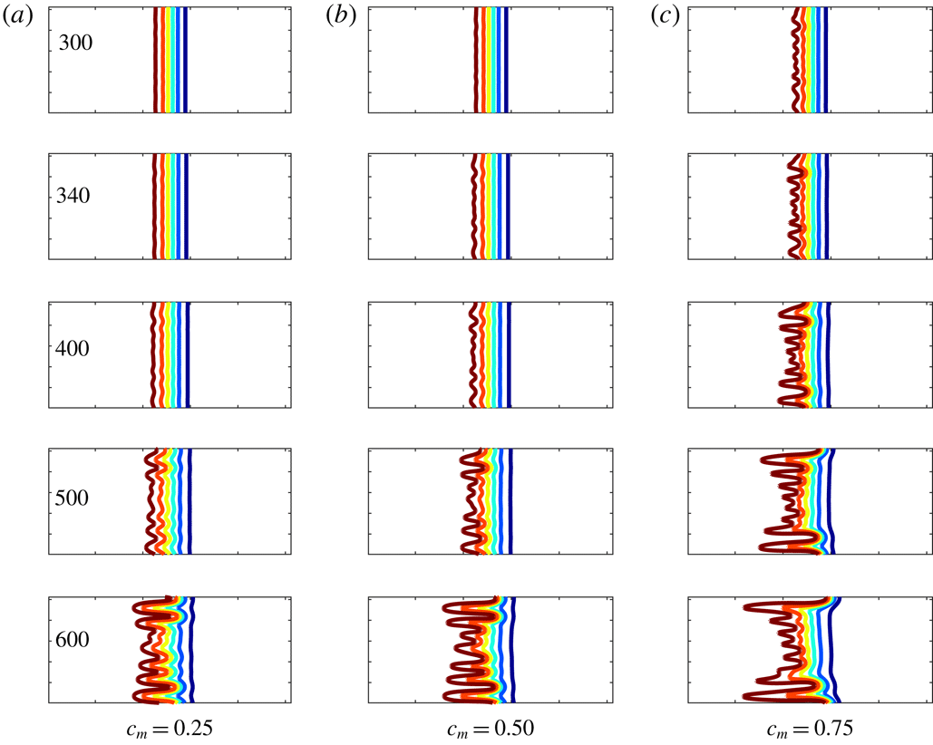
Finger propagation for the set of non-monotonic profiles with
 $\unicode[STIX]{x1D6FC}=5,\unicode[STIX]{x1D707}_{m}=7.5$
and (a)
 $c_{m}=0.25$
, (b)
 $c_{m}=0.5$
and (c)
 $c_{m}=0.75$
. All the simulations have aspect ratio
 $A=4$
. The concentration contours shown span from
 $c^{\prime }=0.1$
to
 $c^{\prime }=0.9$
with six equal increments.

Figure 6 shows the NLS results for
 $\unicode[STIX]{x1D6FC}=5,\unicode[STIX]{x1D707}_{m}=7.5$
and various values of maximum concentration,
 $c_{m}$
. It is observed that at time
 $t=300$
the fingers are visible for
 $c_{m}=0.75$
, whereas the times at which the fingers are visible for
 $c_{m}=0.5$
and
 $c_{m}=0.25$
are
 $t=340$
and
 $400$
, respectively. From this important visual observation it can clearly be noted that the onset of the fingers is early for the higher value of
 $c_{m}$
in comparison to smaller values of
 $c_{m}$
, or in other words, onset of fingers is a monotonically decreasing function of
 $c_{m}$
. These results are consistent with the onset of instability in the linear regime determined from NMA (see figure 4). Further, in contrast to the monotonic viscosity–concentration profiles, in the case of non-monotonic viscosity–concentration profiles, the fingers propagate faster in the backward direction than in the forward direction. This is illustrated in figure 6 where the fingers have spread farther to the left than to the right, especially for the case
 $c_{m}=0.75$
. This result is consistent with the nonlinear simulations of Manickam & Homsy (Reference Manickam and Homsy1994), who refer to this phenomenon as reverse fingering.
The mechanism of reverse fingering, as shown in figure 6, can be explained from the spatial variation of viscosity, which is shown in figure 3(b). For flow systems with such profiles, there would develop a potentially unstable region, where the viscosity increases in the flow direction, followed by a potentially stable region in the downstream direction, where the viscosity decreases in the flow direction. Thus, for non-monotonic displacements the stable zone of the viscosity profiles acts as a barrier for the forward growth of fingers, which, when viewed in a reference moving with the front, tend to propagate backwards. This feature of reverse fingering in the non-monotonic displacement is also illustrated in the analysis of the structure of optimal perturbations, shown in figure 5. Thus, it can be concluded that NMA successfully captures the early evolution of perturbations which is well aligned with results of NLS.
3.2 Stability analysis for favourable endpoint viscosity contrast
In this case, we have
 $\unicode[STIX]{x1D6FC}<1$
, equivalently,
 $\unicode[STIX]{x1D707}_{1}>\unicode[STIX]{x1D707}_{2}$
: the displacing fluid is more viscous than the displaced fluid. The spatial variation of the viscosity profile and the corresponding variation with concentration are shown in figures 7(a) and 7(b), respectively. The flow systems as illustrated in figure 7 are said to have a favourable viscosity contrast, as a high viscosity fluid displaces a low viscosity fluid. As before, in order to compare our results with the existing literature, we use the following parameters:
 $\unicode[STIX]{x1D6FC}=0.5,\unicode[STIX]{x1D707}_{m}=2$
and
 $c_{m}=0.25,0.5$
and
 $0.75$
. With this configuration, the flow has a viscosity ratio of
 $2$
across the weaker unstable zone and a viscosity ratio of
 $2/0.5=4$
across the stable zone.
For
 $\unicode[STIX]{x1D6FC}=0.5$
and
 $\unicode[STIX]{x1D707}_{m}=2$
, (a) the spatial variation of the viscosity profile, (b) viscosity–concentration profiles for
 $c_{m}=0.25,0.5$
and
 $0.75$
. Across the unstable zone, viscosity increases by a factor
 $2$
, while it decreases by a factor of
 $4$
through the stable zone. However, the strength of the (un)stable zone depends on
 $\text{d}\unicode[STIX]{x1D707}/\text{d}c$
, not on the endpoint viscosity ratio. Thus, for the same values of
 $\unicode[STIX]{x1D6FC}$
and
 $\unicode[STIX]{x1D707}$
, different
 $c_{m}$
determine the strength of the two zones.

3.2.1 Optimal amplification
For
 $\unicode[STIX]{x1D6FC}=0.5,k=0.06$
and
 $\unicode[STIX]{x1D707}_{m}=2$
, figure 8 demonstrates the influence of the position of maximal concentration,
 $c_{m}$
, on the optimal amplification,
 $G(t)$
. For the present case, the stability parameter
 $\unicode[STIX]{x1D712}$
has values
 $-10.81,-1.68$
and
 $5.29$
for
 $c_{m}=0.25,0.5$
and
 $0.75$
, respectively. For unfavourable viscosity contrast,
 $\unicode[STIX]{x1D712}>0$
represents the slope of the viscosity profile at the point
 $c=1$
being steeper than at the point
 $c=0$
, whereas
 $\unicode[STIX]{x1D712}<0$
denotes the reverse scenario. From table 1, it can be observed that the length of the stable interval is decided by the parameter
 $c_{m}$
, i.e. longer stable zones with larger values of
 $c_{m}$
. This affects the delay in the onset time,
 $t_{on}$
, as
 $c_{m}$
increases. For
 $\unicode[STIX]{x1D6FC}=0.5$
,
 $c_{m}=0.25$
and
 $0.75$
, an important feature resembling the secondary instability of the optimal amplification
 $G(t)$
is observed. Figure 8(a) illustrates that initially there is an influence of steeper viscosity profile (see figure 7
b) which helps to amplify the energy, but due to the weak unstable region, this energy is only sustained for a transient period. However, when diffusion becomes weaker and the isocontours in the unstable zone overcome the stable zone, then there is a growth of energy which sets the instability and we call this a secondary instability. This temporal evolution of the perturbation was not observed for
 $c_{m}=0.5$
. Further, it is noted that the energy amplification is lowest for
 $c_{m}=0.5$
in comparison to
 $c_{m}=0.25$
and
 $0.75$
. The reason for this secondary instability is due to the steep viscosity gradient at either end at
 $c=0$
or
 $c=1$
for
 $c_{m}=0.25$
and
 $0.75$
. This also shows that the value of
 $c_{m}$
alone is not sufficient to describe the early-time temporal evolution of the disturbances.
For
 $\unicode[STIX]{x1D6FC}=0.5,\unicode[STIX]{x1D707}_{m}=2$
, (a) optimal amplification,
 $G(t)$
, for
 $k=0.06$
with three different values of
 $c_{m}$
. The black dots (●) denote the onset of instability,
 $t_{on}$
. (b) Onset time,
 $t_{on}$
, is monotonically increasing with an increase in
 $c_{m}$
.

For
 $\unicode[STIX]{x1D6FC}=0.5,k=0.06$
and
 $\unicode[STIX]{x1D707}_{m}=2$
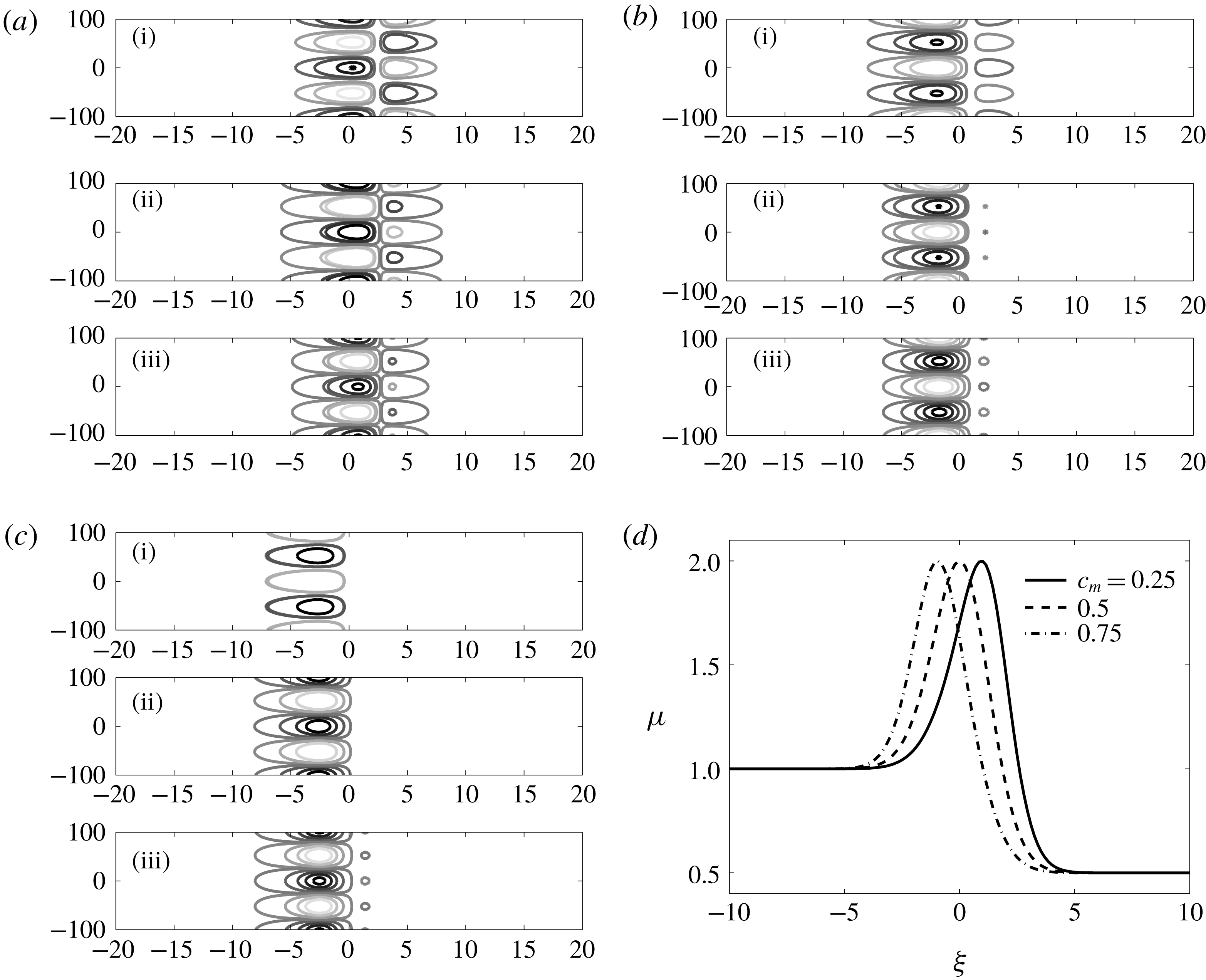
, (a–c) the evolution of the optimal initial perturbations,
 $c_{p}^{\prime }=V_{opt}\cos (ky)$
, for
 $c_{m}=0.25,0.5$
and
 $0.75$
, respectively. Here the time integration intervals are
 $(\text{i})=[0.01,50],(\text{ii})=[0.01,100]$
and
 $(\text{iii})=[0.01,150]$
. The concentration contours shown span from its minimum to maximum values in five equal increments. The initial interface is located at
 $\unicode[STIX]{x1D709}=0$
. Black lines correspond to negative contours and grey lines correspond to positive contours. (d) The spatial variation of viscosity for the same values of
 $\unicode[STIX]{x1D6FC}$
and
 $\unicode[STIX]{x1D707}_{m}$
.

3.2.2 Structure of optimal perturbations
The argument based on the fact that the flow will be unstable if the destabilizing isocontours are stronger than the stabilizing one may not fully describe the physical phenomena in the non-monotonic viscosity–concentration profiles. To have a comprehensive analysis, we have studied the perturbation structures for
 $\unicode[STIX]{x1D6FC}=0.5,k=0.06$
and
 $\unicode[STIX]{x1D707}_{m}=2$
, as shown in figure 9. From this figure, it can be observed that the displacement is stable for all the values of
 $c_{m}$
, but there are no stabilizing right isocontours for
 $c_{m}=0.75$
at time
 $t=50$
. This is in contrast to the argument of Manickam & Homsy (Reference Manickam and Homsy1993). The perturbation contours always have two rows of patches of opposite sign on opposite sides of the viscosity maximum for
 $c_{m}=0.25$
and
 $0.5$
. This can be explained from table 1 as follows: if the recirculating fluid regions extend beyond the unstable region, the left column contours have taken the stabilizing role, which is the case when
 $c_{m}=0.75$
, as shown in figure 9(c). Thus, we conclude that the strength of the destabilizing perturbation contour regions, their location and their interaction with the gradients in the viscosity profile all influence the stability in the case of non-monotonic viscosity–concentration profiles. Further, it is shown in figure 9(b) that, at early times, the right side stabilizing contours are weakened at
 $t=100$
in comparison to
 $t=50$
, which at later time,
 $t=150$
, again strengthened. For this reason, the optimal amplification
 $G(t)$
for
 $c_{m}=0.5$
always has the lowest energy (see the continuous line in figure 8
a).
3.3 Comparison with quasi-steady-state modal analysis
In this section, we present the stability analysis based on the quasi-steady-state approximation in the self-similar
 $(\unicode[STIX]{x1D709},t)$
-domain, which we abbreviate as SS-QSSA (Pramanik & Mishra Reference Pramanik and Mishra2013). Kim & Choi (Reference Kim and Choi2011) used QSSA2 for quasi-steady analysis in the
 $(\unicode[STIX]{x1D709},t)$
domain. In the SS-QSSA approach, the space and time dependences can be separated by fixing the time at
 $t_{0}$
and the disturbance quantities from equation (2.21) are assumed to be
 $$\begin{eqnarray}\displaystyle (\unicode[STIX]{x1D719}_{c},\unicode[STIX]{x1D719}_{u})(\unicode[STIX]{x1D709},t)=(\unicode[STIX]{x1D719}_{c}^{\unicode[STIX]{x1D709}},\unicode[STIX]{x1D719}_{u}^{\unicode[STIX]{x1D709}})(\unicode[STIX]{x1D709})\text{e}^{\unicode[STIX]{x1D70E}(t_{0})t}, & & \displaystyle\end{eqnarray}$$
where
 $\unicode[STIX]{x1D70E}(t_{0})$
is the perturbation (quasi-steady) growth rate at the time
 $t_{0}$
, and
 $\unicode[STIX]{x1D719}_{c}^{\unicode[STIX]{x1D709}}$
and
 $\unicode[STIX]{x1D719}_{u}^{\unicode[STIX]{x1D709}}$
are the concentration and velocity perturbations, respectively. Substituting (3.3) into (2.27)–(2.28) produces an eigenvalue problem for eigenvalues
 $\unicode[STIX]{x1D70E}$
and eigenfunctions
 $\unicode[STIX]{x1D719}_{c}^{\unicode[STIX]{x1D709}}$
, where
 ${\mathcal{L}}$
is as in (2.27). It is noted that here we are presenting the temporal stability analysis, i.e. the non-dimensional wavenumber
 $k$
, as a real number, whereas, the growth rate,
 $\unicode[STIX]{x1D70E}(t_{0})$
, can be allowed to be a complex number. Numerically, the temporal stability analysis has been performed by computing the leading eigenvalues, i.e.
 $\unicode[STIX]{x1D70E}(t_{0})=\max \text{Re}[\unicode[STIX]{x1D6EC}({\mathcal{L}})]$
, the spectral abscissa of the stability matrix
 ${\mathcal{L}}(t_{0})$
. Here
 $\unicode[STIX]{x1D6EC}$
denotes the set of all discrete eigenvalues of
 ${\mathcal{L}}$
. It is observed that the SS-QSSA eigenfunctions are concentrated around the base state. However, these concentration eigenfunctions fail to capture the quadruple structure and, consequently, only predict the temporal growth of disturbances after an initial transient period.
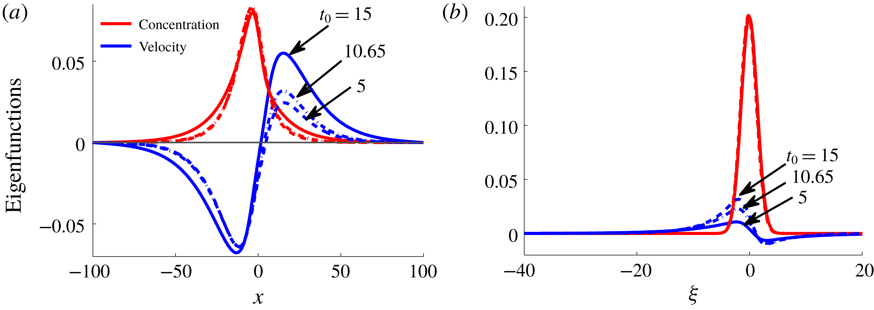
Quasi-steady eigenfunctions,
 $\unicode[STIX]{x1D719}_{c}^{\unicode[STIX]{x1D709}}$
, of the linearized operator
 ${\mathcal{L}}$
(see equation (3.4)) for
 $\unicode[STIX]{x1D6FC}=5,\unicode[STIX]{x1D707}_{m}=7.5,k=0.2$
:
 $c_{m}=0.25$
(a),
 $0.5$
(b) and
 $0.75$
(c), at different frozen times.

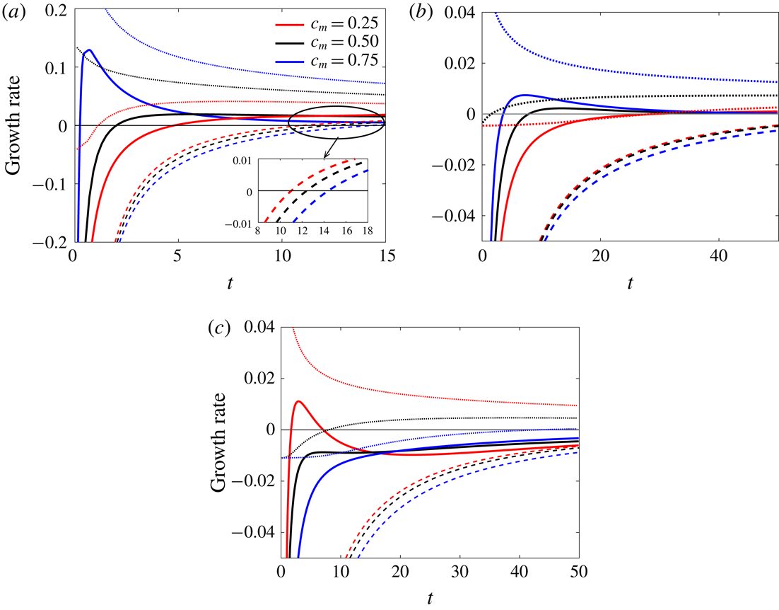
Growth rate for the corresponding viscosity profiles (2.14) with (a)
 $\unicode[STIX]{x1D6FC}=5,\unicode[STIX]{x1D707}_{m}=7.5$
and
 $k=0.2$
, (b)
 $\unicode[STIX]{x1D6FC}=1,\unicode[STIX]{x1D707}_{m}=2$
and
 $k=0.06$
, and (c)
 $\unicode[STIX]{x1D6FC}=0.5$
,
 $\unicode[STIX]{x1D707}_{m}=2$
and
 $k=0.1$
: the growth rate determined from NMA (continuous lines), SS-QSSA (dashed lines) and QSSA (dotted lines). The NMA growth rates are determined from
 $(1/G(t))(\text{d}G(t)/\text{d}t)$
.

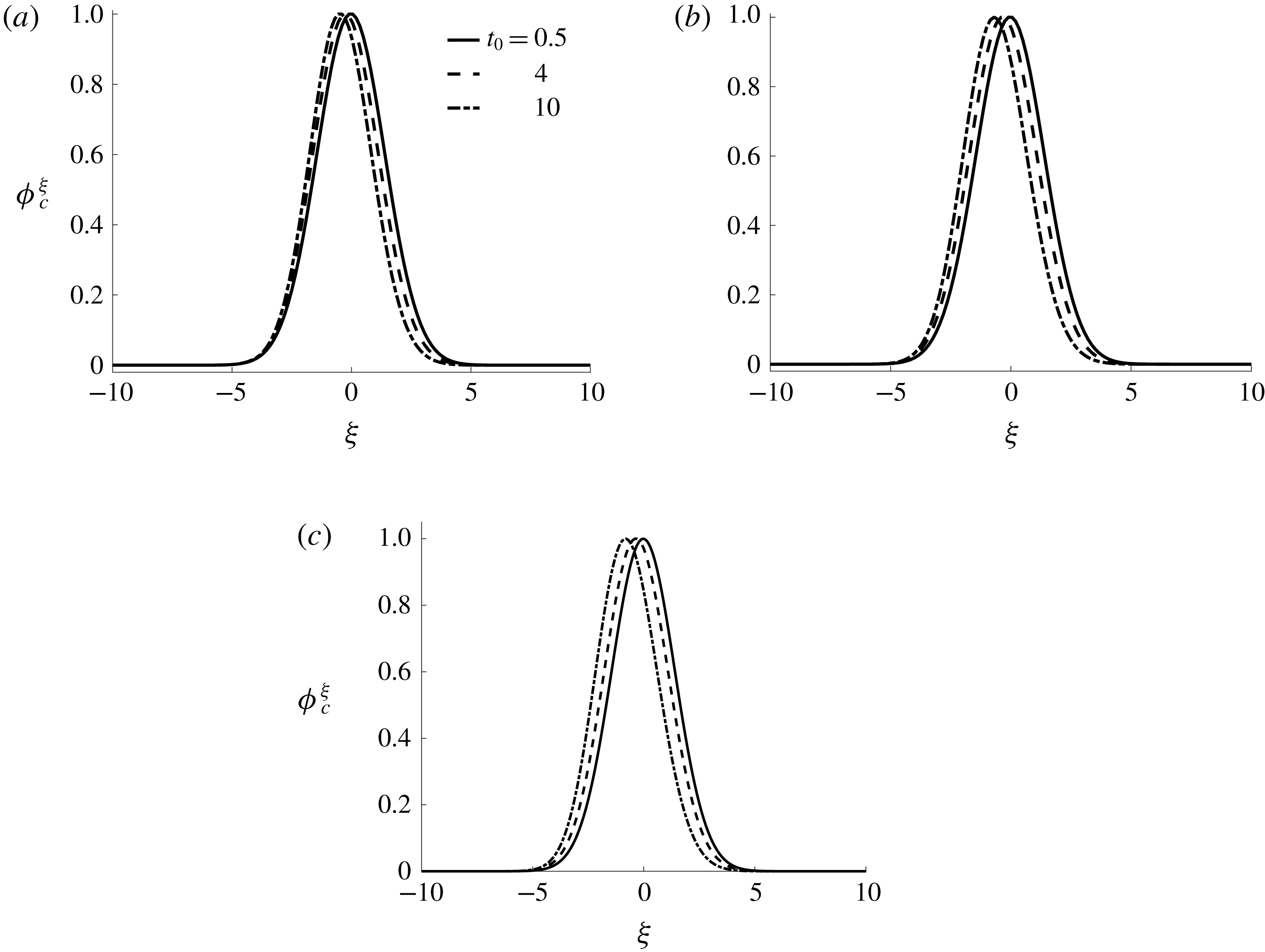
Figure 10 demonstrates the spatial variations of SS-QSSA eigenfunctions at times
 $t_{0}=0.5,4$
and
 $10$
. The parameters used are
 $\unicode[STIX]{x1D6FC}=5,\unicode[STIX]{x1D707}_{m}=7.5,k=0.2$
and
 $c_{m}=0.25,0.5$
and
 $0.75$
. It is observed that SS-QSSA typically produces the dominant eigenfunctions that are qualitatively very different from the corresponding optimal initial perturbations, e.g. the typical quadruple structure of perturbations that are obtained from NMA (see figure 5) are not captured by SS-QSSA eigenfunctions, as evident from figure 10(a–c). A comparison of quasi-steady eigenfunctions in
 $(x,t)$
and
 $(\unicode[STIX]{x1D709},t)$
domains are discussed in appendix B.
With this substantial difference in the structure of the quasi-steady eigenfunctions in comparison to the optimal perturbations, we move to compare the growth rate determined from NMA and SS-QSSA. The growth rate in SS-QSSA can obtained by analysing the spectral abscissa,
 $\unicode[STIX]{x1D70E}({\mathcal{L}})$
, which is defined as the collection of numbers
 $\unicode[STIX]{x1D70E}(t_{0})$
satisfying
 $$\begin{eqnarray}\displaystyle {\mathcal{L}}(t_{0})\unicode[STIX]{x1D719}_{c}^{\unicode[STIX]{x1D709}}=\unicode[STIX]{x1D70E}(t_{0})\unicode[STIX]{x1D719}_{c}^{\unicode[STIX]{x1D709}}, & & \displaystyle\end{eqnarray}$$
where
 $t_{0}$
is the frozen time at which
 $\unicode[STIX]{x1D70E}(t_{0})$
is determined.
Figure 11 illustrates the growth rate obtained from SS-QSSA, QSSA and NMA. In figure 11(a–b), for
 $\unicode[STIX]{x1D6FC}=5$
and
 $1$
, it is observed that the temporal evolution of growth rates determined from NMA and SS-QSSA are opposite to each other. Although both NMA and SS-QSSA predict that the system is unconditionally stable at early times, the SS-QSSA approach illustrates that the onset of instability is an increasing function of
 $c_{m}$
, which is in contrast to the result of NMA (see figure 4
b). At the early times, the qualitative nature of the growth rate of perturbations determined from NMA (continuous lines) and QSSA (dotted lines) are similar. Manickam & Homsy (Reference Manickam and Homsy1993) used the QSSA and suggested that when the parameter
 $\unicode[STIX]{x1D712}$
(see (2.18)) is positive, the flow is always unstable, and when
 $\unicode[STIX]{x1D712}$
is negative, the initially stable flow becomes unstable as the base flow diffuses. For the parameters given in figure 11(a),
 $\unicode[STIX]{x1D712}=-2.12,3.58$
and
 $14.05$
, for
 $c_{m}=0.25,0.5$
and
 $0.75$
, respectively. However, the flow is stable for both
 $\unicode[STIX]{x1D712}>0$
and
 $\unicode[STIX]{x1D712}<0$
. Thus, it is observable that QSSA underpredicts the onset of instability for
 $c_{m}=0.5$
and
 $0.75$
. Furthermore, for
 $\unicode[STIX]{x1D6FC}=5$
, the trend of onset obtained from NMA is in agreement with the NLS results (see figure 6), where it is shown that the onset of fingering is early with the increase in values of
 $c_{m}$
. This suggests that the deviation of the structure of discrete eigenfunctions and eigenvalues from the optimal initial perturbations and non-modal growth, at small times, is primarily due to the non-orthogonality of the quasi-steady eigenmodes. For
 $\unicode[STIX]{x1D6FC}=0.5$
, figure 11(c) depicts that the growth rate of perturbation decreases with increase in
 $c_{m}$
irrespective of any linear stability analysis (QSSA, SS-QSSA and NMA). One important point that can be noted from figure 11(c) is that the system can be unstable as predicted by NMA for
 $c_{m}=0.25$
as opposed to SS-QSSA, in which the system is always stable for the given parameters.
Further, in order to validate the advantage of the non-modal approach, we compare the results of NMA with those of nonlinear simulations (NLS). We obtained the growth rate of concentration perturbations by introducing a sinusoidal perturbation of the form
 $$\begin{eqnarray}c^{\prime }(x,y,t_{0})=\left\{\begin{array}{@{}ll@{}}\unicode[STIX]{x1D716}\cos (ky), & x=x_{i},\\ 0, & \text{otherwise}.\end{array}\right.\end{eqnarray}$$
where
 $x_{i}$
is the position of unperturbed interface,
 $k$
is the non-dimensional wavenumber,
 $t_{0}$
is the time when perturbations are introduced and
 $\unicode[STIX]{x1D716}$
is the amplitude of the perturbation, which is taken as
 $10^{-3}$
. See appendix A for more detail.
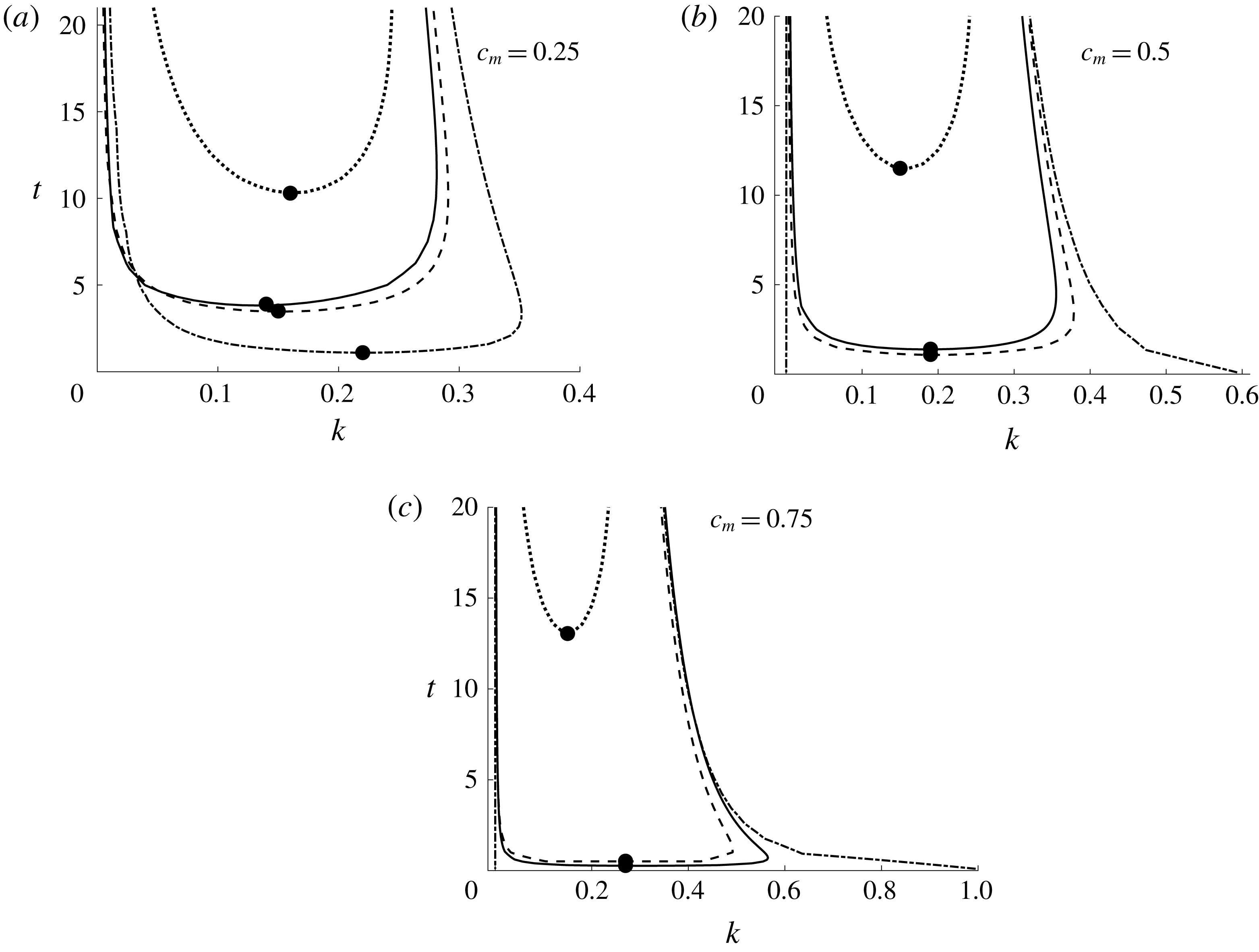
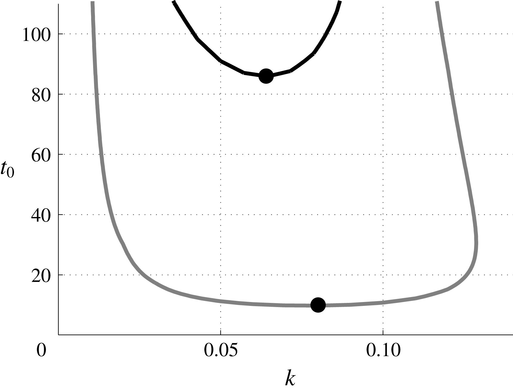
Comparison of neutral curves obtained from SS-QSSA (dotted line), NMA (continuous line), NLS (dashed line) and QSSA (dash-dotted line) for
 $\unicode[STIX]{x1D6FC}=5,\unicode[STIX]{x1D707}_{m}=7.5$
:
 $c_{m}=0.25$
(a),
 $0.5$
(b) and
 $0.75$
(c). The lowest points of each of these curves, marked with the solid dots (●), correspond to the critical wavenumber
 $k_{c}$
and critical time
 $t_{c}$
.

Figure 12 demonstrates the neutral curves obtained from SS-QSSA (dotted line), NMA (continuous line), NLS (dashed line) and QSSA (dash-dotted line), in the
 $(k,t)$
plane. The neutral curves show the combinations of
 $k$
and
 $t$
for which
 $\unicode[STIX]{x1D70E}=0$
. The area above each curve determines the unstable region whereas the region below shows the stable region. The solid dots (●) mark the critical points
 $(k_{c},t_{c})$
at which perturbations initially become unstable. Here the critical time is
 $t_{c}\equiv \min \{\unicode[STIX]{x1D70F}:\unicode[STIX]{x1D70E}(\unicode[STIX]{x1D70F})\geqslant 0,\forall k\}$
and the critical wavenumber is
 $k_{c}\equiv \min \{k:\unicode[STIX]{x1D70E}(t_{c})=0\}$
. In figure 12, we observe that the SS-QSSA analysis predicts qualitatively very different behaviour from the rest of the neutral curves, i.e. SS-QSSA predicts that with an increase in the value of
 $c_{m}$
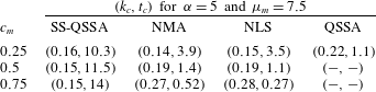
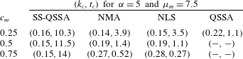
, the stable region increases, in contrast to the other methods. Although QSSA analysis qualitatively agrees with NLS and NMA results, some of the perturbations that are judged unstable by QSSA turned out to be stable, as shown in figure 12(b,c). In table 2 it is shown that at the critical time, the unstable region and dominant wavenumbers determined from NLS and NMA show excellent agreement. It is also observed that NMA and NLS results show that the critical wavenumber
 $k_{c}$
is an increasing function and the critical time
 $t_{c}$
is a decreasing function of
 $c_{m}$
, which are in contrast to the results obtained from SS-QSSA. It can be noted here that when discussing the physical relevance of QSSA analyses, it is important to recall that, in physical systems, perturbations usually arise due to noise that excites many eigenmodes simultaneously. Consequently, modal analyses only predict which perturbations will dominate after an initial transient period. For this reason we have found that QSSA, NMA and NLS results are almost identical at later times.
The critical time,
 $t_{c}\equiv \min \{\unicode[STIX]{x1D70F}:\unicode[STIX]{x1D70E}(\unicode[STIX]{x1D70F})\geqslant 0,\forall k\}$
, and critical wavenumber,
 $k_{c}\equiv \min \{k:\unicode[STIX]{x1D70E}(t_{c})=0\}$
, from each of the neutral curves illustrated in figure 12. The onset times determined from NMA and NLS are indistinguishable. Further, for
 $c_{m}=0.5$
and
 $0.75$
, QSSA shows that the system becomes unstable immediately.
Hence, it can be concluded that irrespective of viscosity–concentration profile, the quasi-steady eigenvalues do not predict the accurate growth rate at early times. To analyse the early spatial and temporal evolution of the perturbations, NMA is a suitable approach. Our main focus in the present article is on determining the onset of instability and describing the physical mechanism of instability. Thus, the effect of injection-driven flow and the influence of lifting in the presence of non-monotonic viscosity profiles may not be directly incorporated. However, we are hoping to explore these effects in the near future.
4 Conclusion
The influence of the non-monotonic viscosity–concentration relationship on miscible displacements in porous media is studied for the rectilinear flows. Due to the time dependence of the stability matrix, we have used the non-modal linear stability (NMA) approach based on the singular value decomposition of the propagator matrix. This approach by construction accommodates all types of initial conditions and hence gives the optimal amplification and optimal perturbation structure. Based on the non-modal linear stability analysis, the non-monotonic viscosity–concentration relationships, proposed by Manickam & Homsy (Reference Manickam and Homsy1993), are characterized by the three parameters, namely, endpoint viscosity contrast, maximum viscosity,
 $\unicode[STIX]{x1D707}_{m}$
, and the concentration that maximizes the viscosity,
 $c_{m}$
. The stability results are interpreted in detail, based on the optimal concentration perturbations. This is in marked contrast to Manickam & Homsy (Reference Manickam and Homsy1993) who used the vorticity perturbation to describe the stability mechanism. Further, the NMA results demonstrate that each of the three parameters has a significant influence on the onset of instability and the shape of eigenfunctions. We notice that since a less viscous fluid displaces a more viscous fluid, an increase in the maximum concentration,
 $c_{m}$
, generally leads to a more unstable flow. This result is in contrast with earlier linear stability results based on eigenanalysis (Kim & Choi Reference Kim and Choi2011). Further, we have observed that the sign of the parameter
 $\unicode[STIX]{x1D712}$
is not helpful in characterizing the dynamics of perturbation growth, whereas the reverse scenario is observed when a more viscous fluid displaces a less viscous fluid. Hence, our findings suggest that the onset and the dynamics of the disturbances obtained by previous investigators, using quasi-steady approximation and eigenanalysis, can be misleading. Moreover, the present analysis describes the physical mechanism which is studied using the singular value decomposition of the propagator matrix, and is in accordance with the nonlinear simulations of Manickam & Homsy (Reference Manickam and Homsy1993, Reference Manickam and Homsy1994). It can be concluded that, for non-monotonic viscosity profiles, the NMA approach can describe the onset of instability and the underlying physical mechanism of instability more accurately. Furthermore, the present linear stability analysis can be helpful in understanding the effect of non-monotonic viscosity profiles in miscible reactive flows (Hejazi et al.
Reference Hejazi, Trevelyan, Azaiez and De Wit2010) and double diffusive convection (Mishra et al.
Reference Mishra, Trevelyan, Almarcha and De Wit2010).
Appendix A. Growth rate from Fourier pseudo-spectral method
Streamfunction forms for the dimensionless equations (2.5)–(2.7) in a Lagrangian frame of reference moving with the speed
 $U$
in the downstream direction are
 $$\begin{eqnarray}\left.\begin{array}{@{}c@{}}\displaystyle \unicode[STIX]{x1D6FB}^{2}\unicode[STIX]{x1D713}=-\frac{\text{d}\ln (\unicode[STIX]{x1D707})}{\text{d}c}\left[\unicode[STIX]{x1D735}\unicode[STIX]{x1D713}\boldsymbol{\cdot }\unicode[STIX]{x1D735}c+\frac{\unicode[STIX]{x2202}c}{\unicode[STIX]{x2202}y}\right],\\ \displaystyle \frac{\unicode[STIX]{x2202}c}{\unicode[STIX]{x2202}t}+\frac{\unicode[STIX]{x2202}\unicode[STIX]{x1D713}}{\unicode[STIX]{x2202}y}\frac{\unicode[STIX]{x2202}c}{\unicode[STIX]{x2202}x}-\frac{\unicode[STIX]{x2202}\unicode[STIX]{x1D713}}{\unicode[STIX]{x2202}x}\frac{\unicode[STIX]{x2202}c}{\unicode[STIX]{x2202}y}=\unicode[STIX]{x1D6FB}^{2}c.\end{array}\right\}\end{eqnarray}$$
For the base state
 $\boldsymbol{u}_{b}=(0,0)$
(equivalently
 $\unicode[STIX]{x1D713}_{b}=$
constant) and
 $c_{b}=(1/2)[1-\text{erf}(x/2\sqrt{t})]$
, introduce an infinitesimal perturbations,
 $\unicode[STIX]{x1D713}=\unicode[STIX]{x1D713}_{b}+\unicode[STIX]{x1D713}^{\prime }$
and
 $c=c_{b}+c^{\prime }$
to (A 1). The associated boundary conditions are given by
 $$\begin{eqnarray}\left.\begin{array}{@{}c@{}}(c^{\prime },\unicode[STIX]{x1D713}^{\prime })(x,y,t)=(0,0),\text{ at }x=0\text{ and }A\,Pe,\\ (c^{\prime },\unicode[STIX]{x1D713}^{\prime })(x,y,t)=(0,0),\text{ at }y=0\text{ and }Pe,\end{array}\right\}\end{eqnarray}$$
where
 $Pe$
is the Péclet number,
 $A=L/H$
is the aspect ratio, and
 $L$
and
 $H$
are the length and width of the computational domain, respectively. We have adopted the Fourier pseudo-spectral method to solve the system (A 1) subject to the boundary conditions (A 2) and initial condition (3.5). Then, we obtained the spatio-temporal evolution of the perturbation quantities,
 $c^{\prime }(x,y,t)$
, and calculated the growth rates associated with the concentration perturbations (Kumar & Homsy Reference Kumar and Homsy1999; Hota et al.
Reference Hota, Pramanik and Mishra2015b
),
 $$\begin{eqnarray}\unicode[STIX]{x1D70E}(t)=\frac{1}{2E(t)}\frac{\text{d}E(t)}{\text{d}t},\end{eqnarray}$$
where the amplification measure is given by
 $E(t)=\int _{0}^{A\,Pe}\int _{0}^{Pe}(c^{\prime }(x,y,t))^{2}\,\text{d}x\,\text{d}y$
. Following Hota et al. (Reference Hota, Pramanik and Mishra2015b
) we have used (A 3) to quantify the growth rate of disturbances and the onset of instability from nonlinear simulations.
Appendix B. Transformation of growth rate from
 $(\unicode[STIX]{x1D709},t)$
coordinates to
$(x,t)$
coordinates


We define an energy
 $E_{1}(t)$
by
 $$\begin{eqnarray}\displaystyle E_{1}(t)={\textstyle \frac{1}{2}}\Vert c_{1}(t)\Vert _{2}^{2}, & & \displaystyle\end{eqnarray}$$
where
 $c_{1}$
is the concentration perturbation in the
 $(x,t)$
coordinate and
 $\Vert \cdot \Vert _{2}$
denotes the norm on
 $L^{2}(-\infty ,\infty )$
, i.e.
 $\Vert f(t)\Vert _{2}^{2}=\int _{-\infty }^{\infty }f^{2}(x,t)\,\text{d}x$
. The growth rate corresponding to the energy
 $E_{1}(t)$
is defined as
 $\unicode[STIX]{x1D70E}_{1}(t)=(1/E_{1}(t))(\text{d}E_{1}(t)/\text{d}t)$
. Now, using the self-similar transformations
 $\unicode[STIX]{x1D709}(x,t)=x/2\sqrt{t}$
and the chain rule
 $\unicode[STIX]{x2202}/\unicode[STIX]{x2202}t|_{(x,t)}=\unicode[STIX]{x2202}/\unicode[STIX]{x2202}t|_{(\unicode[STIX]{x1D709},t)}-(\unicode[STIX]{x1D709}/2t)\unicode[STIX]{x2202}/\unicode[STIX]{x2202}\unicode[STIX]{x1D709}|_{(\unicode[STIX]{x1D709},t)}$
, we have
 $$\begin{eqnarray}\displaystyle \frac{\text{d}E_{1}(t)}{\text{d}t} & = & \displaystyle \frac{1}{2}\int _{-\infty }^{\infty }\frac{\unicode[STIX]{x2202}c_{1}^{2}}{\unicode[STIX]{x2202}t}\,\text{d}x=\int _{-\infty }^{\infty }c_{1}\frac{\unicode[STIX]{x2202}c_{1}}{\unicode[STIX]{x2202}t}\,\text{d}x\nonumber\\ \displaystyle & = & \displaystyle \int _{-\infty }^{\infty }c_{2}\frac{\unicode[STIX]{x2202}c_{2}}{\unicode[STIX]{x2202}t}\,\text{d}\unicode[STIX]{x1D709}-\int _{-\infty }^{\infty }\frac{\unicode[STIX]{x1D709}}{2t}c_{2}(\unicode[STIX]{x1D709},t)\frac{\unicode[STIX]{x2202}c_{2}}{\unicode[STIX]{x2202}\unicode[STIX]{x1D709}}\,\text{d}\unicode[STIX]{x1D709},\end{eqnarray}$$
where
 $c_{2}$
is the concentration perturbation in the
 $(\unicode[STIX]{x1D709},t)$
coordinate and the associated energy is given by
 $E_{2}(t)=(1/2)\int _{-\infty }^{\infty }c_{2}^{2}(\unicode[STIX]{x1D709},t)\,\text{d}\unicode[STIX]{x1D709}$
. Thus, we have
 $$\begin{eqnarray}\displaystyle \frac{\text{d}E_{1}(t)}{\text{d}t} & = & \displaystyle \frac{\text{d}E_{2}(t)}{\text{d}t}-\int _{-\infty }^{\infty }\frac{\unicode[STIX]{x1D709}}{2t}c_{2}(\unicode[STIX]{x1D709},t)\frac{\unicode[STIX]{x2202}c_{2}}{\unicode[STIX]{x2202}\unicode[STIX]{x1D709}}\,\text{d}\unicode[STIX]{x1D709}\nonumber\\ \displaystyle & \Rightarrow & \displaystyle \frac{1}{E_{1}(t)}\frac{\text{d}E_{1}(t)}{\text{d}t}=\frac{1}{E_{2}(t)}\frac{\text{d}E_{2}(t)}{\text{d}t}-\frac{1}{E_{2}(t)}\int _{-\infty }^{\infty }\frac{\unicode[STIX]{x1D709}}{2t}c_{2}\frac{\unicode[STIX]{x2202}c_{2}}{\unicode[STIX]{x2202}\unicode[STIX]{x1D709}}\,\text{d}\unicode[STIX]{x1D709}\nonumber\\ \displaystyle & \Rightarrow & \displaystyle \unicode[STIX]{x1D70E}_{1}(t)=\unicode[STIX]{x1D70E}_{2}(t)-\frac{1}{E_{2}(t)}\int _{-\infty }^{\infty }\frac{\unicode[STIX]{x1D709}}{2t}c_{2}\frac{\unicode[STIX]{x2202}c_{2}}{\unicode[STIX]{x2202}\unicode[STIX]{x1D709}}\,\text{d}\unicode[STIX]{x1D709},\end{eqnarray}$$
where
 $\unicode[STIX]{x1D70E}_{2}(t)=(1/E_{2}(t))(\text{d}E_{2}(t)/\text{d}t)$
is the growth rate in the
 $(\unicode[STIX]{x1D709},t)$
coordinate.
Figure 13 demonstrates the neutral curves, i.e.
 $\unicode[STIX]{x1D70E}_{i}=0,i=1,2$
, for
 $\unicode[STIX]{x1D6FC}=1,c_{m}=0.4$
and
 $\unicode[STIX]{x1D707}_{m}=2$
. The lowest point of each of these curves, marked with the solid dots (●), corresponds to the critical time,
 $t_{c,i}$
, and critical wavenumber,
 $k_{c,i}$
. The dissimilarities between the critical wave numbers (critical time)
 $k_{c,1}$
and
 $k_{c,2}$
(similarly
 $t_{c,1}$
and
 $t_{c,2}$
) are apparent.
Comparison of the SS-QSSA (black line) and QSSA (grey line) neutral curves for
 $\unicode[STIX]{x1D6FC}=1,c_{m}=0.4$
and
 $\unicode[STIX]{x1D707}_{m}=2$
. The critical points
 $(0.08,10)$
and
 $(0.064,86)$
, shown as solid dots (●), are obtained respectively from QSSA and SS-QSSA. It is illustrated that both the onset of instability and the corresponding critical wavenumber are significantly different for QSSA and SS-QSSA.

For the viscosity profile
 $\unicode[STIX]{x1D6FC}=1,\unicode[STIX]{x1D707}_{m}=2,k=0.1$
and
 $c_{m}=0.4$
, quasi-steady eigenfunctions obtained from (a) QSSA and (b) SS-QSSA, for the least stable eigenvalue at different times,
 $t_{0}$
.

Appendix C. Quasi-steady eigenmodes of linear stability matrix
${\mathcal{L}}(t)$

In order to study the physical destabilizing mechanism involved in non-monotonic viscosity profiles, Manickam & Homsy (Reference Manickam and Homsy1993) examined the evolution of the eigensolutions of
 ${\mathcal{L}}(t)$
at freezing times
 $t_{0}$
known as the quasi-steady-state approxi- mation (QSSA). In contrast to Manickam & Homsy (Reference Manickam and Homsy1993), we have analysed the evolution of eigenmodes in the self-similar coordinates
 $(\unicode[STIX]{x1D709},t)$
. To compare the SS-QSSA eigenmodes to those obtained by Manickam & Homsy (Reference Manickam and Homsy1993), we choose the following parameters:
 $k=0.1,\unicode[STIX]{x1D6FC}=1,\unicode[STIX]{x1D707}_{m}=2,$
and
 $c_{m}=0.4$
. The eigenfunctions associated with concentration and velocity perturbations obtained from QSSA and SS-QSSA are shown in figure 14 and the velocity contour plots are illustrated in figure 15. From these two figures it can be concluded that the eigenfunctions in the
 $(\unicode[STIX]{x1D709},t)$
coordinates are localized around the interface whereas the eigenfunctions in
 $(x,t)$
span the whole spatial domain, i.e. these eigenfunctions are global modes. This is the reason why some of the profiles that are judged unstable by the QSSA analysis could turn out to be stable in SS-QSSA or in NMA. Further, the physical mechanism of fingering instability at early times can be studied by analysing the velocity eigenfunctions instead of concentration eigenfunctions.
For the viscosity profile
 $\unicode[STIX]{x1D6FC}=1,\unicode[STIX]{x1D707}_{m}=2,k=0.1$
and
 $c_{m}=0.4$
, contours of quasi-steady velocity eigenfunctions obtained from (a) QSSA and (b) SS-QSSA, for the least stable eigenvalue at different times
 $t_{0}$
. From top to bottom,
 $t_{0}=5,10.65,15$
. The positive perturbations are plotted with black lines and the negative perturbations with grey lines. The velocity contours shown span from the minimum values of to the maximum values of velocity with four equal increments.

Appendix D. Quantifying the non-orthogonality of quasi-steady eigenmodes
The extended duration of the transient period can be illustrated by analysing the interaction of non-orthogonality of the quasi-steady eigenfunctions. To measure the non-orthogonality, let us consider the Gram matrix
 $\unicode[STIX]{x1D648}$
, which is defined as (Bhatia Reference Bhatia1997)
 $$\begin{eqnarray}\unicode[STIX]{x1D648}=\left(\begin{array}{@{}cccc@{}}\langle f_{1},f_{1}\rangle & \langle f_{1},f_{2}\rangle & \ldots & \langle f_{1},f_{n}\rangle \\ \langle f_{2},f_{1}\rangle & \langle f_{1},f_{2}\rangle & \ldots & \langle f_{1},f_{n}\rangle \\ \vdots & \vdots & \vdots & \vdots \\ \langle f_{1},f_{1}\rangle & \langle f_{1},f_{2}\rangle & \ldots & \langle f_{1},f_{n}\rangle \end{array}\right),\end{eqnarray}$$
where
 $\langle f_{i},f_{j}\rangle =\int _{-\infty }^{\infty }f_{i}(x,t)\overline{f_{j}}(x,t)\,\text{d}x$
,
 $\overline{f_{j}}$
denote the complex conjugate of the vector and
 $\{\,f_{j}:j=1,2,\ldots ,n\}$
represents either concentration or velocity perturbations. It is clear that if the set of vectors
 $\{f_{j}:j=1,2,\ldots ,n\}$
forms an orthogonal set, then
 $\unicode[STIX]{x1D648}$
is a unitary matrix and the condition number of
 $\unicode[STIX]{x1D648}$
, denoted by
 $\text{cond}(\unicode[STIX]{x1D648})$
, must be
 $1$
or nearly
 $1$
. But if any two eigenfunctions are non-orthogonal (they may be linearly independent), then
 $\text{cond}(\unicode[STIX]{x1D648})$
can be a very large number. In such cases, the stability analysis investigated from the eigenmodes is either incorrect or suboptimal (Schmid Reference Schmid2007).
For the viscosity profile
 $\unicode[STIX]{x1D6FC}=1,\unicode[STIX]{x1D707}_{m}=2$
and
 $c_{m}=0.4$
, condition number of Gram matrix
 $\unicode[STIX]{x1D648}$
considering first six quasi-steady velocity eigenfunctions obtained from SS-QSSA.

Figure 16 illustrates the change in
 $\text{cond}(\unicode[STIX]{x1D648})$
with respect to
 $t_{0}$
and
 $k$
for
 $\unicode[STIX]{x1D6FC}=1$
,
 $\unicode[STIX]{x1D707}_{m}=2$
and
 $c_{m}=0.4$
. It is observed that at early times the condition number is as large as of order
 $O(10^{10})$
. This shows that at early times the velocity eigenfunctions are not orthogonal, which leads to the disagreement between the onset of instability determined from NMA and SS-QSSA as depicted in figure 11(b). Moreover, the non-orthogonality tends to persist for a longer period of time for small wavenumbers.