Introduction
There are many parameters in agriculture that change over time in a sigmoid pattern. These parameters are divided into two groups. The first includes parameters that are intrinsically increased sigmoidally as a function of time, e.g. plant height (Xiangxiang et al. Reference Xiangxiang, Quanjiu, Jun, Lijun and Xinlei2014; Gajanayake et al. Reference Gajanayake, Raja Reddy and Shankle2015), dry matter (DM) (Moustakas et al. Reference Moustakas, Akoumianakis and Passam2011; Sepaskhah et al. Reference Sepaskhah, Fahandezh-Saadi and Zand-Parsa2011; Shabani et al. Reference Shabani, Sepaskhah and Kamgar-Haghighi2013), leaf growth (Auzanneau et al. Reference Auzanneau, Huyghe, Escobar-Gutiérrez, Julier, Gastal and Barre2011), fruit growth (Génard & Huguet Reference Génard and Huguet1996; Tarara et al. Reference Tarara, Blom, Shafii, Price and Olmstead2009), nitrogen uptake by above-ground plant parts (Moustakas et al. Reference Moustakas, Akoumianakis and Passam2011), calcium accumulation in fruit (Montanaro et al. Reference Montanaro, Dichio, Xiloyannis and Celano2006) and phloem tube number (Feller et al. Reference Feller, Favre, Janka, Zeeman, Gabriel and Reinhardt2015). The second group includes parameters where the accumulative value of their variation increases sigmoidally as a function of time, e.g. accumulative spore germination (Gabriel et al. Reference Gabriel y Galán, Prada, Martínez-Calvo and Lahoz-Beltrá2015), accumulative number of inflorescence (Gur et al. Reference Gur, Osorio, Fridman, Fernie and Zamir2010) and accumulative seed germination (Lim et al. Reference Lim, Awan, Sta. Cruz and Chauhan2015). There are many equations that have sigmoidal patterns, i.e. logistic, Gompertz and Richards (Archontoulis & Miguez Reference Archontoulis and Miguez2015). These equations have one inflection point. The growth rate increases before the inflection point and decreases after it. Therefore, these equations have two phases: before and after the inflection point. Therefore, these equations, known as the singular sigmoid function, can be used for processes with two growth phases. There are some processes in agriculture with more than two growth phases, e.g. normalized difference vegetation index (NDVI) time-series for leaf expansion and senescence (Soudani et al. Reference Soudani, le Maire, Dufrêne, François, Delpierre, Ulrich and Cecchini2008), berry growth of vine (Greer & Weston Reference Greer and Weston2010), fruit water content (Montanaro et al. Reference Montanaro, Dichio, Xiloyannis and Celano2006), peach fruit growth (Génard & Huguet Reference Génard and Huguet1996) and disease progress (Hau et al. Reference Hau, Amorim and Bergamin Filho1993). These processes include two stages and each stage has two phases, like a singular sigmoid. The double sigmoid function is the mathematical model that describes these processes. Indeed, the double sigmoid function is formed from the sum of two different singular sigmoid functions, i.e. logistic–logistic, logistic–Gompertz and Gompertz–Gompertz (Hau et al. Reference Hau, Amorim and Bergamin Filho1993; Lipovetsky Reference Lipovetsky2010). The double logistic equation, which is one form of the double sigmoid function, is used in the current study. This equation, similar to other double sigmoid equations, has two inflection points for two growth stages. As shown in Fig. 1, there is a phase with zero or constant growth between two growth stages. For plant growth, e.g. winter wheat, winter rye, winter triticale, winter rapeseed and winter barley, this phase occurs in the cold period of winter. Metabolic activity and DM production are low during the cold period. Similar to the double logistic equation, winter cereals and rapeseed have two growth stages, before and after the cold period. Therefore, the double logistic equation can be used to simulate the growth of plants that tolerate a cold period.
Double logistic curve. Each stage has an inflection point that growth rate is maximum at that point.

In the current study, the double logistic equation was used to describe the growth of rapeseed under water stress.
Materials and methods
Theoretical principal
As mentioned above, the double logistic function is formed from the sum of two single logistic equations as follows (Lipovetsky Reference Lipovetsky2010):
 $$Y - Y_{{\rm min}} = \displaystyle{{Y_{{\rm mid}} - Y_{{\rm min}}} \over {1 + {\rm exp}( - ax + b)}} + \displaystyle{{Y_{{\rm max}} - Y_{{\rm mid}}} \over {1 + {\rm exp}( - cx + d)}}$$
where Y is the dependent variable, i.e. DM, x is the independent variable, i.e. time or growing degree day (GDD), Y min, Y mid and Y max are the minimum, intermediate and maximum dependent variables, respectively, exp is the exponential function and a, b, c and d are constant coefficients. For plant growth, Y min and Y max are equal to the DM at the start and end of growing season, respectively. In other words, Y min is the weight of planted seeds and Y max is the DM weight at harvesting. For the symmetric double logistic curve, Y mid is equal to (Y min + Y max)/2. For winter cereals and rapeseed, growth is not symmetric and plant growth before the cold period is lower than after it. Therefore, Y mid is not the DM at the end of the first growing period (beginning of the cold period) and it is also not equal to (Y min + Y max)/2. However, DM at the time of cold period is related to (Y max − Y mid). Each stage has an inflection point and growth rate is maximum at that point. The value of this point is equal to d/c and b/a for the first and second growing periods, respectively. The length of slow growth period during winter is related to both b/a and d/c. The initial plant growth rate is high and increases from planting to the first inflection point. After the first inflection point, as the air temperature decreases, the growth rate decreases until the onset of slow growth period during winter. In Eqn (1), since a and c have positive values, Y′ [Eqn (2)] is >zero. This implies that Eqn (1) is a strictly increasing function. This means that in the cold period, the growth rate is near zero. This is in accordance with field conditions, where the growth rate is very low. In spring, as the air temperature increases, plant growth starts again and the growth rate increases until the second inflection point. After the second inflection point, the growth rate decreases until harvest, when the growth rate is zero.
A derivative of Eqn (1) shows the growth rate as follows:
 $$\eqalign{Y{\rm ^{\prime}} & = \displaystyle{{(Y_{{\rm mid}} - Y_{{\rm min}})a{\rm exp}( - ax + b)} \over {{(1 + {\rm exp}( - ax + b))}^2}} \cr & + \displaystyle{{(Y_{{\rm max}} - Y_{{\rm mid}})c{\rm exp}( - cx + d)} \over {{(1 + {\rm exp}( - cx + d))}^2}}}$$
There are two times during the growing season where the growth rate is maximum. These maximum growth rates take place at the inflection points of the equation.
To consider different environmental conditions in the growing season and planting dates, cumulative heat units (GDD) can be used instead of days after planting (DAP). Growing degree days are calculated by the following equation:
 $$GDD = \mathop \sum \nolimits (T_{{\rm av}} - T_{{\rm base}})$$
where T av is the daily average of air temperature (°C) and T base is the base temperature (°C) below which plant growth is zero. Base temperature for rapeseed was considered as 5 °C (Morrison et al. Reference Morrison, McVetty and Shaykewich1989).
Field experiment
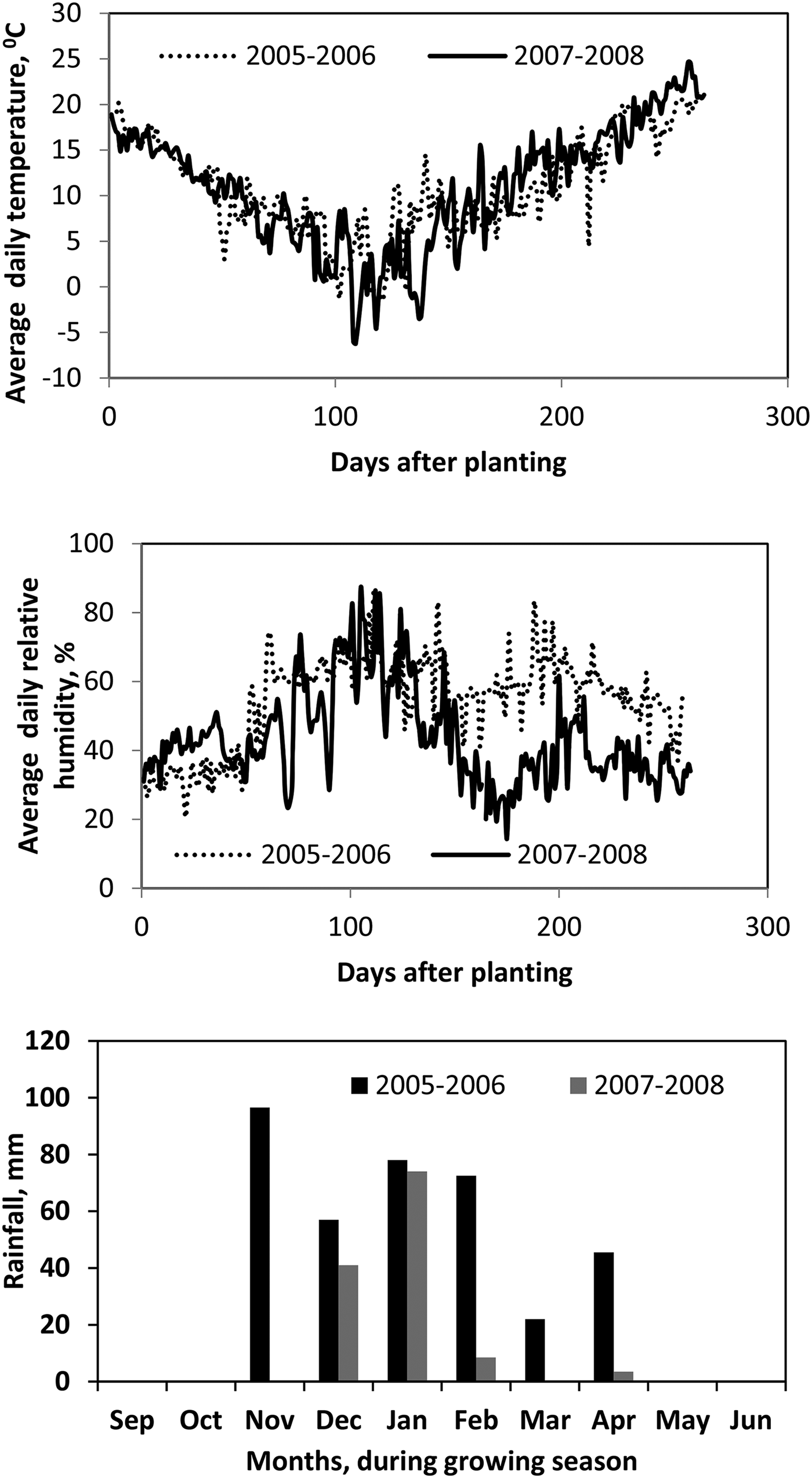
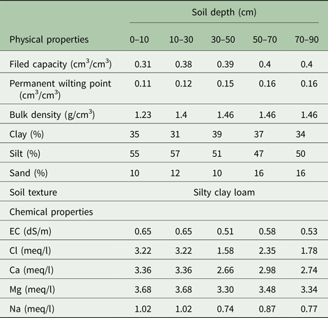
The data used in the current investigation were obtained from experimental data published by Shabani et al. (Reference Shabani, Kamkar Haghighi, Sepaskhah, Emam and Honar2009) and Honar et al. (Reference Honar, Sabet Sarvestani, Shams, Sepaskhah and Kamgar Haghighi2013). These experiments were conducted to study the effect of water stress on physiological parameters in a silty clay loam soil [Fine, carbonatic, mesic, Typic Calcixerepts (Soil Survey Staff 1993)] at the Experimental Research Station in the Agricultural College, Shiraz University, I. R. of Iran (29°36′N, 52°33′E, 1810 m a.s.l.), during 2005/06 and 2007/08. All conditions of the two experiments (e.g. treatments, rapeseed cultivar and field properties) were similar. Physical and chemical properties of soil and water are shown in Table 1. Average daily temperature, daily relative humidity and total rainfall of the region for the two experimental years are shown in Fig. 2.
Average daily temperature, average daily relative humidity and total rainfall of region for 2 years.

Soil physical and chemical properties of the experimental site

The experimental trial was a random block design, with five treatments and four replications. Treatments were: full irrigation at all growth stages (I1), water stress during the vegetative stage in early spring at BBCH 30–59 (Lancashire et al. Reference Lancashire, Bleiholder, Van Den Boom, Langelüddecke, Stauss, Weber and Witzenberger1991) (I2), water stress during the flowering and podding stages at BBCH 60–79, (I3), water stress during the grain filling and ripening stages at BBCH 80–99 (I4) and rain-fed (I5) treatment with supplemental irrigation at time of planting. The dimension of each plot was 3 × 5 m2 and distance between two adjacent plots was 1.0 m to prevent water invasion from one plot to another. The winter rapeseed cultivar Licord was planted, which is tolerant to drought stress. Seeds were planted on 23 September 2005 and 22 September 2007 in five rows with spacing between rows of 0.5 m. The seed planting rate was 8.0 kg/ha (160 seeds/m2). Ammonium phosphate fertilizer at a rate of 100 kg/ha and urea at a rate of 50 kg product/ha were mixed with the soil at ploughing with an additional 100 kg/ha of urea applied in spring at BBCH 50 (BBCH 1997). With exception of a drought stress period, the irrigation interval was about 7–10 days and before each irrigation event, soil water content at depths of 0.2, 0.3, 0.6, 0.9 and 1.2 m was measured with a Neutron Probe [CPN 503 DR, CPN International, Concord, CA, USA]. Soil water content in the root zone was used to determine the amount of net irrigation water as calculated by the following equation:
 $$d_n = \mathop \sum \limits_{i = 1}^n (\theta _{\,fci} - \theta _i)\Delta z_i$$
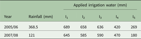
where d n is the net irrigation water depth (m), θ fci and θ i are the volumetric soil water content in layer i at field capacity and before irrigation, respectively (m3/m3), Δz is the soil layer thickness (m) and n is the number of soil layers. Amounts of irrigation water applied for different irrigation treatments and rainfall is presented in Table 2. The volume of irrigation water was obtained by multiplying the irrigation water depth with the area of the plot. The amount of water applied was measured by a volumetric flow meter. The first, second and third irrigation events in all irrigation treatments were similar and used well water for uniform and vigorous seed germination and vegetative stands.
Amount of rainfall and applied irrigation water in different treatments
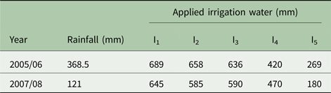
I1 is the full irrigation in all growth stages, I2 is the water stress in a vegetative stage in early spring, I3 is water stress during the flowering and podding stages, I4 is the water stress during grain filling stage, I5 is the rain-fed treatment with supplemental irrigation at time of planting.
To determine the weight of DM of above-ground shoots during the growing season, three plants were selected from each plot and oven-dried at 60 °C for 2 days. After harvest on 7 June 2006 and 10 June 2008, DM was determined from the three central rows with 1.0 m distance from two edges.
The values of the coefficient in Eqn (1) were determined by the Solver tool in MS EXCEL software.
Statistical parameters
To compare the estimated DM with the measured values, goodness of fit indicator (d), normalized root mean square error (NRMSE) and the mean residual error (MRE) were used. These parameters are calculated as follows (Willmott et al. Reference Willmott, Rowe and Mintz1985):
 $$NRMSE = \left[ {\displaystyle{{\sum\nolimits_{i = 1}^n {{(P_i - O_i)}^2}} \over {nO_{{\rm ave}}^2}}} \right]^{0{\cdot}5}$$
 $$d = 1 - \displaystyle{{\mathop \sum \nolimits_{i = 1}^n {(P_i - O_i)}^2} \over {\mathop \sum \nolimits_{i = 1}^n {\left( {\left \vert {P_i - O_{{\rm ave}}} \right \vert + \left \vert {O_i - O_{{\rm ave}}} \right \vert} \right)}^2}}$$
 $$MRE = \displaystyle{{\sum\nolimits_{i = 1}^n {(P_i - O_i)}} \over {nO_{{\rm ave}}^{}}} $$
where P i and O i are the predicted and observed values, respectively, O ave is the mean of measured values, n is the number of data, MRE is a measure of prediction bias, with negative and positive MRE values indicating underestimation and overestimation, respectively. Normalized root mean square error is always a positive value, with low and high values indicating the good and poor performance of the model, respectively. If the value of d is close to 1.0 and the value of NRMSE is close to 0.0, the goodness of fit is better. The estimation is considered excellent if the NRMSE is <0.1, good if the NRMSE is >0.1 and <0.2, fair if the NRMSE is >0.2 and <0.3, and poor if the NRMSE is >0.3 (Jamieson et al. Reference Jamieson, Porter and Wilson1991).
Results
Growth based on days after planting
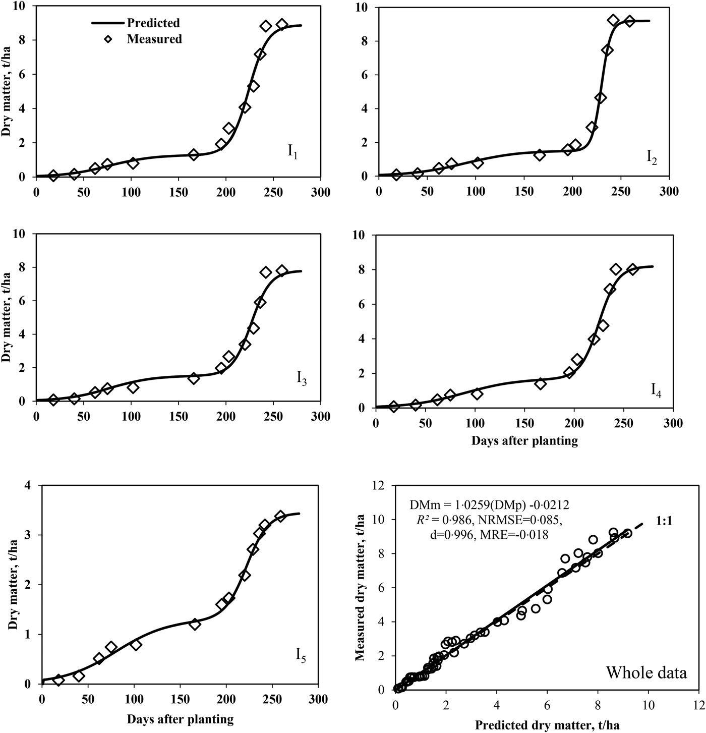
The measured DM of the first year was fitted to Eqn (1). Results are shown in Fig. 3 and Table 3. Results showed that the double logistic equation was fitted accurately to the measured data. Statistical parameters indicated that the double logistic equation was fitted very accurately to data of all irrigation treatments. The value of the goodness of fit (d) is high (0.996) and NRMSE is low (0.085) (Fig. 3, whole data). Results showed that the double logistic model resulted in a slight underestimation (negative MRE) of the DM. As mentioned above, values of b/a and d/c in Eqn (1) are the inflection points before and after a cold period, respectively. Values of the inflection points before and after a cold period are presented in Table 3.
The measured (DMm) and predicted (DMp) dry matter for different irrigation treatments and whole data based on DAP. I1: full irrigation at all growth stages, I2: water stress during the vegetative stage in early spring, I3: water stress during the flowering and podding stages, I4: water stress during the grain filling stage, I5: rain-fed treatment with supplemental irrigation at time of planting, NRMSE: normalized root mean square error, d: goodness of fit, MRE: mean residual error.

Coefficient values of the double logistic equation (Eqn (1)) based on days after planting for dry matter

I1 is the full irrigation in all growth stages, I2 is the water stress in a vegetative stage in early spring, I3 is the water stress during the flowering and podding stages, I4 is the water stress during the grain filling stage, I5 is the rain-fed treatment with supplemental irrigation at time of planting. Inf1 and Inf2 are the inflection points before and after a cold period, respectively.
Growth based on growing degree day
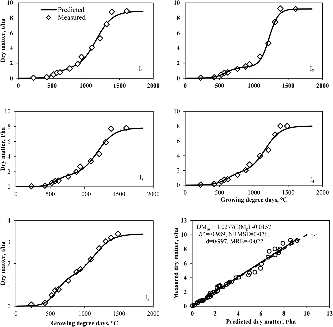
The double logistic equation based on GDD [Eqn (1)] was fitted to the measured DM under different irrigation treatments. Results of the measured and predicted DM are shown in Fig. 4 and Table 4. The relationship between the predicted and measured DM for all treatments and times of measurement are shown in Fig. 4. The value of the goodness of fit (d) is high (0.997) and NRMSE is 0.076. These statistical parameters indicate that there were no significant differences in the fitting of the measured and predicted DM by the double logistic equation for all irrigation treatments. Based on DAP, the slow growth period during winter, which occurred between the two growth stages, was clearly visible (Fig. 3): this was also the case when based on GDD (Fig. 4). This is due to the fact that GDD do not vary during the days that the air temperature is lower than the base temperature.
The measured (DMm) and predicted (DMp) dry matter for different irrigation treatments and whole data based on GDD. I1: full irrigation at all growth stages, I2: water stress during vegetative stage in early spring, I3: water stress during the flowering and podding stages, I4: water stress during the grain filling stage, I5: rain-fed treatment with supplemental irrigation at time of planting, NRMSE: normalized root mean square error, d: goodness of fit, MRE: mean residual error.

Coefficient values of the double logistic equation (Eqn (1)) for dry matter based on growing degree days after planting

I1 is the full irrigation at all growth stages, I2 is the water stress during the vegetative stage in early spring, I3 is the water stress during the flowering and podding stages, I4 is water stress during the grain filling stage, I5 is the rain-fed treatment with supplemental irrigation at time of planting. Inf1 and Inf2 are the inflection points before and after a cold period, respectively.
Growth rate
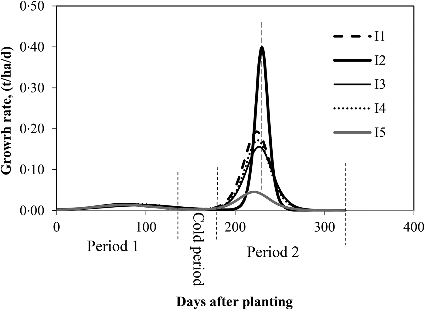
The growth rate in different irrigation treatments was calculated by using the constant coefficient of Eqn (1) (Table 3) and Eqn (2). Results of the growth rate are shown in Fig. 5. Results showed that the growth rate was lower before the cold period than after. There were two maximum growth rates for winter rapeseed. The first occurred before cold period and other after it. There was no difference between growth rates in different irrigation treatments before the cold period. The growth rate was very close to zero during the cold period. Maximum points in Fig. 5 occurred on the same days that the inflection point occurred in Fig. 3. With exception of treatment I2, the start and end times of growth after cold period were similar in other treatments. The minimum growth rate was observed in treatment I5 (rain-fed treatment with supplemental irrigation at time of planting) due to severe water stress during the growing period in spring.
The growth rate in different irrigation treatments. (I1: full irrigation at all growth stages, I2: water stress during the vegetative stage in early spring, I3: water stress during flowering and podding stages, I4: water stress during the grain filling stage, I5: rain-fed treatment with supplemental irrigation at time of planting.).

Application
Relationship between coefficients of the double logistic model and agronomic input parameters
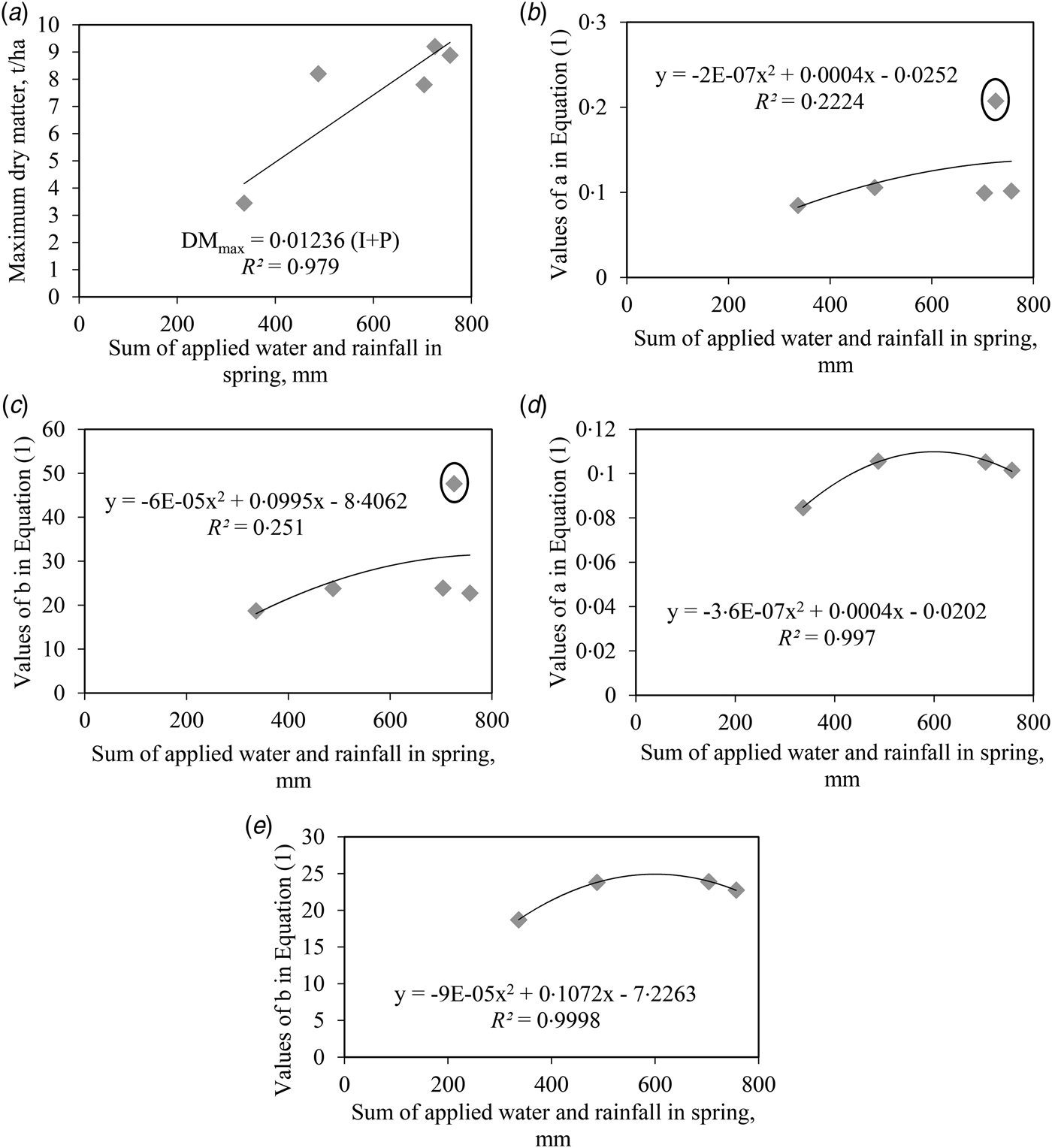
Sepaskhah et al. (Reference Sepaskhah, Fahandezh-Saadi and Zand-Parsa2011) and Shabani et al. (Reference Shabani, Sepaskhah and Kamgar-Haghighi2013) showed that there were relationships between coefficients of the logistic model and the agronomic input parameters (e.g. water, nitrogen and irrigation water salinity). They proposed a relationship for those coefficients as a function of applied water, nitrogen application rate and irrigation water salinity. In the current study, the values of d, c, and Ymid in Eqn (1) were not affected by agronomic management parameters. However, there were relationships between the values of a, b and maximum DM (DMmax) and the sum of seasonal applied water and rainfall during the spring season (I + P). The average values of d, c and (Y max − Y mid) were 0.041, 3.285 and 1.46, respectively. These values can be used for DM simulation. The regression model between the values of DMmax of double logistic equation and sum of seasonal applied water and rainfall in spring is presented as follows (Fig. 6(a)):
 $$\eqalign{& DM_{{\rm max}}\; = \; 0{\cdot}01236(I + P) \cr & \quad R^{\rm 2} = 0{\cdot}{\rm 979},\,{\rm SE = 1}.{\rm 25},\,P_{{\rm value}} \lt 0{\cdot}00{\rm 1}}$$
where I + P is the sum of seasonal applied water and rainfall in spring (67.5 mm). The observed and predicted a and b are shown in Figs 6(b) and (c). The values of a and b for I2 were far from a and b of all the other treatments. These two points are circled in Figs 6(b) and (c) and are omitted in Figs 6(d) and (e). The correlation between the values of a and b of double logistic equation and sum of seasonal applied water and rainfall in spring are presented as follows:
 $$\eqalign{& a\,{\rm =} - 3{\cdot}6 \times 10^{ - 7}({\rm I} + {\rm P})^2{\rm + \;} 0{\cdot}000433({\rm I} + {\rm P}) \cr & - 0{\cdot}02016,\,R^2\,{\rm =}\, 0{\cdot}996,\,{\rm SE =}\, 0{\cdot}0003,\,P_{{\rm value}} \lt 0{\cdot}01} $$
 $$\eqalign{& b\,{\rm =} - 8{\cdot}9 \times 10^{ - 5}({\rm I} + {\rm P})^2{\rm + \;} 0{\cdot}10719({\rm I} + {\rm P}) \cr & - 7{\cdot}2263,\,R^2\,{\rm =}\, 0{\cdot}999,\,{\rm SE =}\, 17{\cdot}95,\,P_{{\rm value}} \lt 0{\cdot}05} $$
The relationship between the values of maximum dry matter (DMmax, a), a (b and d) and b (c and e) of the double logistic equation and sum of seasonal applied water and rainfall in spring.

The DM of rapeseed for similar climatic and agronomy conditions can be determined by using the above relationships.
Evaluation of relationship between coefficients of the double logistic model and agronomic input parameters
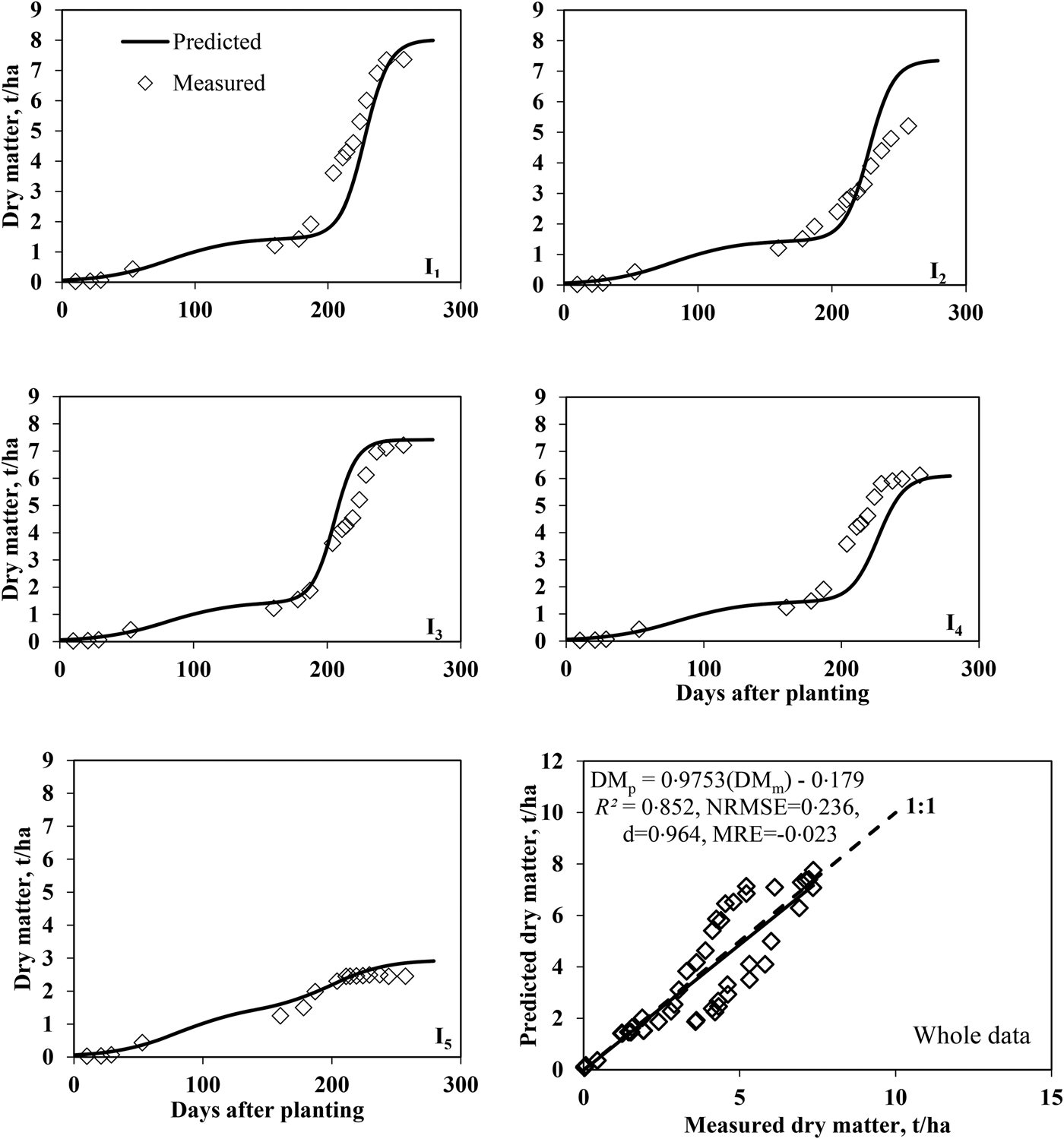
Published data by Honar et al. (Reference Honar, Sabet Sarvestani, Shams, Sepaskhah and Kamgar Haghighi2013) were used to validate Eqs. (8)–(10) to estimate the DM. The results for the measured DM and the DM predicted by the double logistic model for different irrigation treatments are shown in Fig. 7. For all irrigation treatments, comparison of the slope and intercept of the relationship between the measured DM and the DM predicted by the double logistic model (Fig. 7, whole data) using the 1 : 1 line, showed that the slope and intercept are not different from 1.0 and 0.0, respectively.
The measured and predicted dry matter for different irrigation treatments and whole data (evaluation based on published data by Honar et al. (Reference Honar, Sabet Sarvestani, Shams, Sepaskhah and Kamgar Haghighi2013)). I1: full irrigation at all growth stages, I2: water stress during the vegetative stage in early spring, I3: water stress during the flowering and podding stages, I4: water stress during the grain filling stage, I5: rain-fed treatment with supplemental irrigation at time of planting, NRMSE: normalized root mean square error, d: goodness of fit, MRE: mean residual error.

Discussion
The results of the present study showed that the double logistic equation can be fitted accurately to the measured data. There was no difference between the values of d and c in different irrigation treatments before the cold period. This may be due to the fact that water stress occurred in spring and after the cold period. Rainfall occurrence in autumn and winter and irrigation at time of planting for uniform and vigorous seed germination and vegetation stands before and during the cold period prevented water stress occurrence before spring. Variation between the values of d and c in different treatments may have resulted from sampling error. Shabani et al. (Reference Shabani, Kamkar Haghighi, Sepaskhah, Emam and Honar2009) reported that water stress in a vegetative stage in early spring caused delayed vegetative growth after the cold period. However, after a period of water stress, plants had renewed vegetative growth and produced more branches. Similar results were reported by Bouchereau et al. (Reference Bouchereau, Clossais-Besnard, Bensaoud, Leport and Renard1996) and Gan et al. (Reference Gan, Angadi, Cutforth, Potts, Angadi and McDonald2004). For this reason, the inflection point of the second growing period was 230 DAP in water-stressed conditions in the vegetative stage in the early spring treatment (I2) which was later than for the other treatments. An earlier inflection point was observed in rain-fed treatments with supplemental irrigation at time of planting. This may be due to the fact that severe water stress caused a decrease in the length of the growing season. Average DM during the cold period (average (Y max − Y mid) in Table 3) was 1.46 t/ha. Shabani et al. (Reference Shabani, Kamkar Haghighi, Sepaskhah, Emam and Honar2009) reported that there was no significant difference between all treatments for DM during the cold period.
Results showed that the DM predicted by the double logistic model based on GDD was in accordance with the measured data. The DM predicted by the double logistic equation based on GDD was slightly closer to the measured DM compared with DM predicted by the double logistic equation based on DAP, as supported by the lower NRMSE. All points that were stated about the values of coefficients for the DAP case are valid for obtained results for GDD case.
Water stress in the vegetative stage in early spring caused maximum growth rate for all treatments after the cold period. As reported by other investigators (Bouchereau et al. Reference Bouchereau, Clossais-Besnard, Bensaoud, Leport and Renard1996; Gan et al. Reference Gan, Angadi, Cutforth, Potts, Angadi and McDonald2004; Shabani et al. Reference Shabani, Kamkar Haghighi, Sepaskhah, Emam and Honar2009), it seems that occurrence of temporary water stress in early spring resulted in stimulation of vegetative growth after the end of water stress. Also, the time of maximum growth rate occurrence was delayed due to a water stress event in early spring and plant recovery after the end of water stress.
Using data published by Honar et al. (Reference Honar, Sabet Sarvestani, Shams, Sepaskhah and Kamgar Haghighi2013) as independent data to evaluate the equations presented in the current study, it was shown that, with the exception of treatment I2, the double logistic model resulted in a fair estimation of DM. Meteorological data assessments showed that very low rainfall in February, March and April and low relative humidity during the spring season in the second experiment caused more severe drought stress in I2 compared with the first experiment (I1). Therefore, plants had not recovered after the end of the water stress period and DM decreased in the second experiment (I2), in contrast to the first experiment (I1).
For the double logistic equation based on DAP, sowing date is important due to the effect of air temperature on plant growth and DM accumulation before and after the cold period. For the double logistic equation, sowing date is important when crop growth is based on DAP, However, this is not the case when using GDD. Note that the coefficients of the double logistic equation should be calibrated when changing the cultivar and when the regional climate and agronomic parameters are different.
In conclusion, based on results of the current study, the double logistic function can be used to describe and simulate DM production during the growth period of the winter rapeseed. The double logistic function was in accordance with DM production both before and after the cold period. The double logistic equation can also be used to explain the growth rate of winter rapeseed. The results indicated that a double logistic function based on GDD resulted in slightly better DM prediction during the growing season in comparison with that obtained based on the DAP. Therefore, the double logistic function based on GDD or based on the cumulative heat units can be used for different weather conditions and planting dates. The equation obtained in the current study can be used to predict DM of winter rapeseed, however, as it is an empirical model it should be calibrated when changing the cultivar, the regional climate or the agronomic parameters.