





1. Introduction
The presence of adverse pressure gradients (APGs) (Sears & Telionis Reference Sears and Telionis1975) and surface curvature (Bradshaw & Young Reference Bradshaw and Young1973) around streamlined and bluff bodies can give rise to three-dimensional (3-D) separation and associated unsteady instabilities that span multiple frequency bands. The resulting separated flow is highly complex, due to the coupling between the unsteady dynamics of the recirculating region, large-scale coherent motions, incoming turbulence and the competing influences of pressure gradients and curvature. Although these effects jointly determine both the mean and unsteady behaviour, our current physical understanding of 3-D turbulent separation remains incomplete – particularly for flows in which the separation front is not fixed but free to adjust to the local pressure field and curvature. In the present work, we examine the unsteady 3-D dynamics of turbulent separation over the smooth Boeing Gaussian bump with error function shoulders, with an emphasis on explorations of the low-frequency (LF) motions.
Bumps and hills subjected to turbulent boundary-layer inflow (see, e.g. Williams et al. Reference Williams, Annamalai, Ozoroski, Roy and Lowe2022) provide canonical test cases to investigate the combined influence of pressure gradient and surface curvature on smooth-body flow separation, which together produce far more complex dynamics than either in isolation. This challenge has motivated the development of a new generation of benchmark configurations, such as the Gaussian bump (Slotnick Reference Slotnick2019; Williams et al. Reference Williams, Samuell, Sarwas, Robbins and Ferrante2020) and the Benchmark Validation Experiments for RANS and LES Investigations (BeVERLI) hill (Gargiulo et al. Reference Gargiulo, Duetsch-Patel, Ozoroski, Beardsley, Vishwanathan, Fritsch, Borgoltz, Devenport, Roy and Lowe2021), among others, that have been established to improve the modelling and prediction of turbulent separation as part of NASA’s CFD Vision 2030 initiative (Slotnick et al. Reference Slotnick, Khodadoust, Alonso, Darmofal, Gropp, Lurie and Mavriplis2014). The Gaussian bump features a smooth Gaussian profile with a large spanwise aspect ratio (width-to-height,
 $B_w/H\approx 8.3$
), producing a wide separated footprint with pronounced 3-D features (Williams et al. Reference Williams, Samuell, Sarwas, Robbins and Ferrante2020, Reference Williams, Samuell, Robbins, Annamalai and Ferrante2021). The flow behaviour over such geometries is sensitive to shape parameters, particularly the aspect ratio (
 $B_w/H$
) and the relative height of the bump compared with the incoming boundary-layer thickness, which together influence the reorientation of vorticity (Mason & Morton Reference Mason and Morton1987), the distribution of upwash and downwash in the wake and the proportion of mass flux that passes over versus around the body. Related laminar simulations by Cooper et al. (Reference Cooper, Savino, Cooper and Wu2025) further show that spanwise non-uniformity in an imposed APG can produce strongly 3-D separated-flow structure, illustrating one route by which spanwise pressure-gradient variation can influence the separation dynamics. Most of what is currently known about hill-type turbulent separated flows concerns the mean topology; comparatively little is known about the organisation of the unsteady motions that give rise to that mean.
Although the mean topology of hill-type separated flows has been extensively characterised (e.g. Garcia-Villalba et al. Reference Garcia-Villalba, Li, Rodi and Leschziner2009; Williams et al. Reference Williams, Samuell, Robbins, Annamalai and Ferrante2021; Gargiulo et al. Reference Gargiulo, Duetsch-Patel, Ozoroski, Beardsley, Vishwanathan, Fritsch, Borgoltz, Devenport, Roy and Lowe2021; Duetsch-Patel et al. Reference Duetsch-Patel2022; Simmons et al. Reference Simmons, Thomas, Corke and Hussain2022, Reference Simmons, Thomas, Corke and Gluzman2024), it is the underlying unsteady dynamics that govern the body-force fluctuations, organise the Reynolds stresses and mediate the inter-scale energy transfers that ultimately sustain the mean-flow structure. Even in canonical 2-D wakes such as the cylinder at moderate Reynolds numbers
 $\textit {Re}\gt 300$
, the mean flow does not exist instantaneously – the familiar recirculation zone arises from the time-averaged imprint of self-sustained vortex shedding (Williamson Reference Williamson1996). In 3-D smooth-body separations, the situation is considerably more intricate: the separation front and reattachment region undergo broadband motions involving both shear-layer instabilities and large-scale LF unsteadiness (Eaton & Johnston Reference Eaton and Johnston1982; Byun & Simpson Reference Byun and Simpson2006; Weiss et al. Reference Weiss, Mohammed-Taifour and Schwaab2015; Ching & Eaton Reference Ching and Eaton2020). These unsteady dynamics, rather than the mean field alone, determine the exchange of momentum between the separated shear layer, the recirculation zone and the outer boundary layer (Kiya & Sasaki Reference Kiya and Sasaki1983; Driver et al. Reference Driver, Seegmiller and Marvin1987; Wu et al. Reference Wu, Meneveau and Mittal2020). However, most previous studies of hill and bump flows have focused on time-averaged quantities, leaving the nature and spectral organisation of the unsteady motions – particularly those at low frequencies – much less understood.
At high Reynolds numbers, separated turbulent flows exhibit a broad hierarchy of time scales (Eaton & Johnston Reference Eaton and Johnston1982; Hudy et al. Reference Hudy, Naguib, Humphreys and William2003; Weiss et al. Reference Weiss, Mohammed-Taifour and Schwaab2015). In nominally 2-D configurations, two dominant modes are well established. The first is a medium-frequency vortex-shedding mode associated with the roll-up and advection of spanwise vortices (Na & Moin Reference Na and Moin1998b
; Weiss et al. Reference Weiss, Mohammed-Taifour and Schwaab2015), of order
 $St_{L_{\textit{sep}}}=fL_{\textit{sep}}/U_{\infty }=O(10^{-1})$
, with
 $L_{\textit{sep}}$
the mean separation length, where
 $St$
is the Strouhal number,
 $f$
is the frequency and
 $U$
is the freestream velocity. The second is a lower-frequency flapping or breathing mode, corresponding to an oscillatory vertical motion of the separated shear layer (Eaton & Johnston Reference Eaton and Johnston1982; Cherry et al. Reference Cherry, Hillier and Latour1984; Driver et al. Reference Driver, Seegmiller and Marvin1987; Weiss et al. Reference Weiss, Mohammed-Taifour and Schwaab2015; Wang & Ghaemi Reference Wang and Ghaemi2022), typically an order of magnitude slower than the shedding frequency (
 $St_{L_{\textit{sep}}}=O(10^{-2})$
). This LF motion has been described either as flapping – a vertical oscillation of the separated shear layer in geometry-induced turbulent separation bubbles (TSBs) that modulates the reattachment point – or as breathing – a modulation of the size of the recirculation zone in variable-separation TSBs where both separation and reattachment points fluctuate. Although closely related, we use the term breathing in the context of variable-separation flows here to emphasise changes in the separated zone extent rather than a purely kinematic shear-layer deflection. A growing body of work also suggests that, even in nominally 2-D configurations, such LF motions may be manifestations of an underlying 3-D global spanwise stationary mode (Borgmann et al. Reference Borgmann, Cura, Weiss and Little2024; Steinfurth et al. Reference Steinfurth, Li, Scarano and Weiss2025; Fuchs et al. Reference Fuchs, Steinfurth, von, Jakob, Weiss and Oberleithner2026).
In 3-D geometries, additional long time-scale dynamics emerge. In particular, a very-low-frequency (VLF) mode associated with instantaneous asymmetric motions of the wake at
 $St=O(10^{-3})$
has been reported in axisymmetric wakes (Rigas et al. Reference Rigas, Oxlade, Morgans and Morrison2014; Pavia et al. Reference Pavia, Varney, Passmore and Almond2019) and in rectilinear-type bodies such as the Ahmed body, a surface-mounted half-axisymmetric body and the BeVERLI hill (Grandemange et al. Reference Grandemange, Gohlke and Cadot2013; Pavia et al. Reference Pavia, Passmore and Sardu2018; Duetsch-Patel et al. Reference Duetsch-Patel2022; Panesar et al. Reference Panesar, Xia and Passmore2023). This mode is typically one order of magnitude slower than the breathing mode and is associated with a global spanwise instability – either as an azimuthal precession in axisymmetric bodies or as spanwise-bistable switching between mirror-symmetric states in rectilinear ones (Grandemange et al. Reference Grandemange, Cadot and Gohlke2012, Reference Grandemange, Gohlke and Cadot2013; Rigas et al. Reference Rigas, Oxlade, Morgans and Morrison2014; Pavia et al. Reference Pavia, Passmore and Sardu2018; MacGregor et al. Reference MacGregor, Gargiulo, Duetsch-Patel, Lavoie and Lowe2023). The stability of these motions is highly sensitive to geometry: small variations in aspect ratio or base curvature can trigger reflectional-symmetry breaking (Garcia-Villalba et al. Reference Garcia-Villalba, Li, Rodi and Leschziner2009; Grandemange et al. Reference Grandemange, Gohlke and Cadot2013; Duetsch-Patel et al. Reference Duetsch-Patel2022; Panesar et al. Reference Panesar, Xia and Passmore2023).
The present study explores the properties of low/mid-frequency and 3-D unsteady motions on the Gaussian bump using a combination of simultaneously sampled unsteady surface pressures and particle image velocimetry (PIV) in orthogonal planes.
Sections 1.1 and 1.2 review prior observations of unsteady modes in 2-D and 3-D separated flows.
1.1. Unsteadiness in two-dimensional flows
The unsteadiness of turbulent separated flows developing from geometrical singularities – such as backward-facing steps, blunt plates and fence-and-splitter configurations – has been well documented (e.g. Eaton & Johnston Reference Eaton and Johnston1982; Kiya & Sasaki Reference Kiya and Sasaki1983; Cherry et al. Reference Cherry, Hillier and Latour1984; Driver et al. Reference Driver, Seegmiller and Marvin1987; Spazzini et al. Reference Spazzini, Iuso, Onorato, Zurlo, Di and Maria2001). In these flows, the mean streamlines form a recirculation region that reattaches to the wall, defining a TSB (Eaton & Johnston Reference Eaton and Johnston1982; Kiya & Sasaki Reference Kiya and Sasaki1983). This closed bubble topology, however, exists only in the statistical mean: instantaneous realisations exhibit non-reattaching topologies, with continuous mass exchange between the separated region and the outer stream (Kiya & Sasaki Reference Kiya and Sasaki1983; Weiss et al. Reference Weiss, Mohammed-Taifour and Schwaab2015; Wu et al. Reference Wu, Meneveau and Mittal2020). The intermittent opening and closing of this region is associated with unsteady shear-layer motion and global variations in the reverse-flow extent, which are commonly manifested as LF flapping motions in fixed-separation flows, breathing motions in variable-separation flows and medium-frequency vortex-shedding modes (Eaton & Johnston Reference Eaton and Johnston1982; Cherry et al. Reference Cherry, Hillier and Latour1984; Driver et al. Reference Driver, Seegmiller and Marvin1987; Weiss et al. Reference Weiss, Mohammed-Taifour and Schwaab2015; Wang & Ghaemi Reference Wang and Ghaemi2022; Fang & Wang Reference Fang and Wang2024). Across a range of geometry-induced TSBs, the corresponding Strouhal numbers typically fall in the ranges
 $St_{L_{\textit{sep}}}=0.08$
–
 $0.2$
for the flapping mode (Fang & Wang Reference Fang and Wang2024) and
 $0.5$
–
 $1.0$
for the shedding mode (Eaton & Johnston Reference Eaton and Johnston1982; Kiya & Sasaki Reference Kiya and Sasaki1983; Cherry et al. Reference Cherry, Hillier and Latour1984; Na & Moin Reference Na and Moin1998a
; Hudy et al. Reference Hudy, Naguib, Humphreys and William2003; Weiss et al. Reference Weiss, Mohammed-Taifour and Schwaab2015; Wu et al. Reference Wu, Meneveau and Mittal2020). The breathing motion has also been reported in pressure-induced and variable-separation TSBs, with
 $St_{L_{\textit{sep}}}\approx 0.01$
(Weiss et al. Reference Weiss, Mohammed-Taifour and Schwaab2015; Mohammed-Taifour & Weiss Reference Mohammed-Taifour and Weiss2016), and
 $St_{L_{\textit{sep}}}\approx 0.05$
in trailing-edge separations (Wang & Ghaemi Reference Wang and Ghaemi2022).
The flapping mode has been extensively reported in geometry-induced, fixed-separation flows (e.g. Eaton & Johnston Reference Eaton and Johnston1982; Kiya & Sasaki Reference Kiya and Sasaki1983; Cherry et al. Reference Cherry, Hillier and Latour1984; Driver et al. Reference Driver, Seegmiller and Marvin1987). It appears to manifest as vertical oscillations of the separated shear layer, leading to streamwise oscillations of the reattachment point. In APG separations, the freely moving separation front introduces an additional degree of freedom, yielding broadband LF oscillations associated with the TSB expansion and contraction, often termed breathing. Several mechanisms have been proposed to identify potential sources of the flapping (Eaton & Johnston Reference Eaton and Johnston1982; Kiya & Sasaki Reference Kiya and Sasaki1983; Cherry et al. Reference Cherry, Hillier and Latour1984) and breathing modes (Wu et al. Reference Wu, Meneveau and Mittal2020; Wang & Ghaemi Reference Wang and Ghaemi2022; Fang & Wang Reference Fang and Wang2024), and they are the subject of ongoing research. Moreover, it appears that neither the flapping, breathing nor shedding frequencies collapse universally with
 $U_{\infty }/L_{\textit{sep}}$
, since
 $L_{\textit{sep}}$
itself evolves with the unsteady state of the bubble and local shear-layer development (Wu et al. Reference Wu, Meneveau and Mittal2020).
Recent studies on smooth-geometry, nominally 2-D TSBs further show that the LF flapping and breathing motions observed in a symmetry plane in fixed- and variable-separation TSBs, respectively, is often the planar manifestation of an inherently 3-D stationary global mode (Cura et al. Reference Cura, Hanifi, Cavalieri and Weiss2024; Borgmann et al. Reference Borgmann, Cura, Weiss and Little2024; Steinfurth et al. Reference Steinfurth, Li, Scarano and Weiss2025; Cura et al. Reference Cura, Hanifi, Cavalieri and Weiss2025; Fuchs et al. Reference Fuchs, Steinfurth, von, Jakob, Weiss and Oberleithner2026). For wall-mounted humps, Borgmann et al. (Reference Borgmann, Cura, Weiss and Little2024) find that the instantaneous separation location varies only weakly along the surface. In particular, despite being a variable-separation flow, they find that the dominant LF shear-layer dynamics (
 $St_{L_{\textit{sep}}}\lesssim 0.1$
) resemble the flapping mode reported for geometry-induced TSBs, and it is in fact the 2-D projection of a spanwise meandering structure. Using time-resolved PIV and spectral proper orthogonal decomposition (POD), they show that these spanwise-undulating structures possess wavelengths in the range
 $0.62\,L_{\textit{sep}} \lesssim \lambda _y \lesssim 1.26\,L_{\textit{sep}}$
(i.e.
 $\lambda _y = \mathcal{O}(L_{\textit{sep}})$
), extend across the full streamwise length of the TSB, and generate alternating peaks and valleys in the recirculating region. The spatial structure of these 3-D modes – and their associated frequency (
 $St_{L_{\textit{sep}}} \approx 0.1$
, near the lower bound of the geometry-induced TSB flapping range
 $St_{L_{\textit{sep}}} \approx 0.08$
–
 $0.20$
) – is consistent with the dominant eigenfunctions associated with the shear-layer flapping mode observed in the centreline-symmetry plane. Similarly, time-resolved measurements over a smooth backward-facing ramp by Steinfurth et al. (Reference Steinfurth, Li, Scarano and Weiss2025) reveal that the LF band (
 $St_{L_{\textit{sep}}}\lesssim 0.05$
) corresponds to a spanwise-structured meandering mode: a mirror-inverted pattern that is locked in space while oscillating in time, with spanwise wavelength of the order of the channel width,
 $\lambda _y=O(L)$
, and pronounced nodes and antinodes set by the tunnel sidewall confinement. For a straight backward-facing ramp, Fuchs et al. (Reference Fuchs, Steinfurth, von, Jakob, Weiss and Oberleithner2026) used resolvent analysis to show that such stationary spanwise modes can arise from the interference of left- and right-travelling 3-D modes reflected by the tunnel sidewalls, with dominant spanwise wavelengths of several TSB lengths. In both ramp configurations, the streamwise–vertical expansion and contraction observed in the symmetry plane is interpreted as the projection of these spanwise-structured modes whose wavelengths are governed primarily by the spanwise domain size
 $O(L)$
(which is typically several times
 $L_{\textit{sep}}$
). These recent results support the view that the apparently 2-D breathing motion seen in smooth-body separations is often the planar imprint of an underlying 3-D stationary global mode, and that the spanwise domain width,
 $L$
, emerges as a key length scale alongside the mean separation length,
 $L_{\textit{sep}}$
, when interpreting LF unsteadiness.
1.2. Three-dimensional unsteadiness
In addition to the shedding and breathing motions characteristic of 2-D separated flows, 3-D wakes have sometimes been observed to exhibit an additional VLF mode associated with large-scale spanwise or azimuthal unsteady motions of the wake. This motion occurs on time scales one to two orders of magnitude slower than the dominant shedding or breathing motions and represents a defining feature of 3-D turbulent separation. Its form appears to depend strongly on geometry.
Axisymmetric bodies exhibit both axial bubble-pumping motions and a slow azimuthal precession of the wake (Rigas et al. Reference Rigas, Oxlade, Morgans and Morrison2014; Pavia et al. Reference Pavia, Varney, Passmore and Almond2019; Zhang & Peet Reference Zhang and Peet2023; Panesar et al. Reference Panesar, Xia and Passmore2023). For such geometries, the wake may freely precess around the body, admitting an infinite continuum of equivalent asymmetric states corresponding to random rotations of the planar vortex-shedding axis (Rigas et al. Reference Rigas, Oxlade, Morgans and Morrison2014) – i.e. a stochastic meandering along the azimuthal coordinate. The VLF motion originates from a symmetry-breaking bifurcation of the steady axisymmetric wake (Fabre et al. Reference Fabre, Auguste and Magnaudet2008), yielding a planar-symmetric state that subsequently undergoes stochastic precession at
 $St_D \sim 10^{-3}$
(with body diameter
 $D$
) – an order of magnitude slower than the bubble-pumping motion (
 $St_D \sim 10^{-2}$
) and two orders slower than the vortex-shedding mode (
 $St_D \sim 10^{-1}$
) (Pavia et al. Reference Pavia, Varney, Passmore and Almond2019; Zhang & Peet Reference Zhang and Peet2023).
Rectilinear geometries, such as the Ahmed body and the BeVERLI hill, restrict symmetry-breaking modes to reflection about a plane, producing a bistable wake, where the wake switches intermittently between two spanwise-asymmetric states (Grandemange et al. Reference Grandemange, Cadot and Gohlke2012, Reference Grandemange, Gohlke and Cadot2013; Duetsch-Patel et al. Reference Duetsch-Patel2022; MacGregor et al. Reference MacGregor, Gargiulo, Duetsch-Patel, Lavoie and Lowe2023). In such flows, the wake typically dwells for extended periods in one asymmetric configuration before randomly switching to the other.
Despite the different symmetry constraints, both axisymmetric and rectilinear wakes exhibit comparable VLF frequencies (
 $St_D \sim 10^{-3}$
). In contrast, the intermediate bubble-pumping motion (
 $St_D \sim 10^{-2}$
) – well established in axisymmetric and surface-mounted bluff bodies (Pavia et al. Reference Pavia, Passmore and Sardu2018; Panesar et al. Reference Panesar, Xia and Passmore2023) – has not previously been observed in smooth hill- or bump-type configurations.
The discussion above motivates the following key questions that will be addressed in the present study:
-
(i) What are the dominant unsteady modes in the Gaussian bump flow? Specifically, does the flow exhibit the VLF spanwise, breathing, and vortex-shedding modes previously identified in 3-D turbulent separations, and how do their spatial and spectral characteristics compare across these frequency bands?
-
(ii) If observed, what is the nature of the VLF dynamics? In particular, are these motions associated with spanwise fluctuations of the wake, and do they resemble the continuous precessional (meandering) behaviour of axisymmetric wakes or the discrete bistable switching seen in rectilinear bodies?
The remainder of the paper is organised as follows. The geometry and past work on the bump are briefly reviewed in § 2. Section 3 introduces the measurement techniques, experimental set-up and the symmetrisation method used to extract symmetric and antisymmetric velocity components. The mean field is presented in § 4, followed by an analysis of the unsteady dynamics in § 5. A broader discussion of the 3-D unsteady dynamics is provided in § 6, and the key findings are summarised in § 7.
2. The Boeing Gaussian bump
The surface of the Boeing Gaussian bump is defined as
 \begin{align} z(x,y) = \frac {H}{2} \, e^{(-x/x_0)^2} \left [ 1 + \mathrm{erf}\!\left ( \frac {L_b/2 - 2y_0 - |y|}{y_0} \right ) \right ]\!, \end{align}
where
 $x$
,
 $y$
and
 $z$
denote the streamwise, spanwise and vertical directions, respectively. The splitter-plate width is
 $L_b = 35.5'' = 0.9017\,\mathrm{m}$
, defining the geometric parameters
 $x_0 = 0.195\,L_b$
,
 $y_0 = 0.06\,L_b$
and bump height
 $H = 0.085\,L_b = 0.0766\,\mathrm{m}$
. The full-width, half-maximum bump width is
 $B_w = 8.33H = 0.640\,\mathrm{m}$
. Profiles along the two symmetry planes,
 $y/H = 0$
and
 $x/H = 0$
, are shown in figure 1. The wind-tunnel ceiling was located at half the tunnel width above the inflow splitter plate.
Two-dimensional profiles of the Boeing Gaussian bump along the two symmetry planes:
 $(a)$
 $y/H=0$
(flow from left to right);
 $(b)$
 $x/H = 0$
, with annotation of bump width
 $B_w$
.

The geometry is designed to replicate challenges relevant to high-lift wing configurations (
 $H/\delta \sim O(10)$
) and the spanwise taper aims to limit complex sidewall interactions. Williams et al. (Reference Williams, Samuell, Sarwas, Robbins and Ferrante2020) performed oil-film surface flow visualisations on the bump using china clay and kerosene in the
 $3'\times 3'$
Low-Speed Wind Tunnel at the University of Washington, revealing the 3-D nature of the flow. Surface-pressure measurements revealed that the flow is Reynolds-number insensitive in the mean for
 $\textit {Re}_H\,\geqslant \,226\,000$
. The flow is dominated by two counter-rotating surface vortices on either side of the centreline-symmetry plane
 $y/H=0$
. The shear-stress surface pattern resembles the ubiquitous owl-face-of-the-first-kind pattern, consisting of a saddle separation on the centreline that splits into two symmetric foci (nodes) on either side, and another saddle point on the centreline downstream. The two counter-rotating vortices emerge approximately at the location of surface-concavity change (
 $x/H\approx 1.67$
). This pattern was also reproduced by Gray et al. (Reference Gray, Gluzman, Thomas, Corke, Lakebrink and Mejia2021) at a higher Reynolds number (
 $\textit {Re}_H=335\,000$
).
The off-surface-vortex topology of the owl-face-of-the-first-kind was conceptualised by Perry & Hornung (Reference Perry and Hornung1984) – consisting of two vortices emanating from the foci (both of opposite sense) being tilted into forming a streamwise-oriented counter-rotating vortex pair. Recent stereoscopic PIV work by Gray et al. (Reference Gray, Lakebrink, Thomas, Corke, Gluzman and Straccia2023b ) shows agreement with this conceptual picture.
Comparison of experimental and computational results indicates that the bump presents a significant challenge for predicting flow separation, with Reynolds-averaged Navier–Stokes simulations and delayed detached eddy simulations producing a much thinner separation zone, opposite Reynolds-number trends and sometimes asymmetric results (Williams et al. Reference Williams, Samuell, Sarwas, Robbins and Ferrante2020; Gray et al. Reference Gray, Gluzman, Thomas and Corke2021, Reference Gray, Gluzman, Thomas, Corke, Lakebrink and Mejia2022).
Recently, Manohar et al. (Reference Manohar, Williams, Martinuzzi and Morton2023) developed a machine-learning-based technique to temporally super-resolve under-sampled PIV snapshots of the centreline bump flow (
 $\textit {Re}_{H}=226\,000$
) around separation. Their work facilitated the interpretation of motions governing the multiple frequencies measured by the wall-pressure sensors. They found that a vortex-shedding frequency
 $St_{L_{\textit{sep}}}=0.67$
, is present along the centreline plane, and is potentially associated with the formation, agglomeration and advection of large-scale vortical structures. A lower frequency at
 $St_{L_{\textit{sep}}}=0.067$
, present upstream of the separation front and just downstream of the apex at the centreline-symmetry plane, was interpreted to reflect the breathing vertical oscillation of the separated shear layer.
The present work extends these investigations to consider dynamics at the very lowest frequencies observed in the wall-pressure spectra. The analysis characterises the VLF component, examines its relationship to the higher-frequency breathing and shedding motions and evaluates its connection to the bi-stable or meandering behaviour reported in other hill and bluff-body wakes. By combining synchronised wall-pressure and PIV measurements, the work aims to provide a unified description of the multi-frequency dynamics that govern the unsteady separation over the Gaussian bump.
3. Methods
Experiments were conducted in the
 $3'\times 3'$
Low-Speed Wind Tunnel at the University of Washington. A rendering of the Gaussian bump model and the planar PIV configurations in two orthogonal orientations is shown in figure 2. The splitter plate spans
 $L_b = 0.9017\,\mathrm{m} = 11.8\,H$
in width, with adhesive-backed foam strips sealing the gap to the tunnel sidewalls so that the bump spans the full tunnel width
 $L=0.9144\,\mathrm{m} = 11.94\,H$
. The 3D-printed leading-edge section, of length
 $8'' = 0.203\,\mathrm{m} = 2.65\,H$
, follows a 10:1 modified super-ellipse profile and is positioned such that the bump apex (
 $x=0$
) lies one plate width
 $L$
downstream of the stagnation point. A 240-grit sandpaper strip located at
 $x = -0.778\,L = -9.28\,H$
serves as a tripping device to ensure a fully turbulent boundary layer. The stagnation point was set just above the geometric leading edge using a
 $12'' = 0.305\,\mathrm{m} = 3.98\,H$
trailing-edge flap deflected by
 $7^{\circ }$
, whose angle was set by comparing pressure taps symmetrically placed either side of the leading edge. The free-stream velocity,
 $U_{\infty }$
, was monitored using an Omega PX653–10D5V differential pressure transducer measuring the static pressure difference between the inlet and test-section entrance. The transducer was calibrated using a pitot static tube above the plate at the boundary-layer measurement location. Boundary-layer mean velocity profiles were obtained at
 $x = -0.43\,L = -5.13\,H$
using a Pitot probe on a traversing mechanism (Williams et al. Reference Williams, Samuell, Sarwas, Robbins and Ferrante2020), and the corresponding parameters are listed in table 1. Each dataset comprises synchronised high-rate wall-pressure and planar PIV measurements, acquired at multiple orthogonal planes as described in the following subsections. The inflow Reynolds number was chosen as surface-pressure measurements were found to be
 $\textit {Re}$
-invariant in the mean for
 $\textit {Re}_H \geqslant 226\,000$
(Williams et al. Reference Williams, Samuell, Sarwas, Robbins and Ferrante2020).
Inflow and boundary-layer characteristics;
 $U_{\infty }$
the free-stream speed measured,
 $\delta$
is the 99 % thickness of the incoming boundary layer and
 $\theta$
its momentum thickness. Measurement details are provided in Williams et al. (Reference Williams, Samuell, Sarwas, Robbins and Ferrante2020). The nominal Reynolds number based on
 $U_{\infty }$
and the bump height,
 $H\,=\,0.0766$
m, is
 $\textit {Re}_H\,=\,2.26\times 10^{5}$
.

Table 1. Long description
A table with one row and six columns summarizing inflow and boundary-layer characteristics. The columns are labeled as follows: U infinity in meters per second, H delta, H theta, Re theta, Re H, and Re L. The row contains the following values: 45, 12.7, 106, 2100, 226000, and 2.70 times 10 to the power of 6.
3.1. Instrumentation set-up
Static wall pressure was measured at 25 surface locations (figure 4) using AllSensors D1-P4V miniature amplified differential pressure transducers with full-scale ranges of 5ʹʹ and 10ʹʹ
 $\mathrm{H_2O}$
. All pressure taps were drilled normal to the surface with a diameter of
 $1/32'' = 0.79\,\mathrm{mm}$
, onto which 2ʹʹ (
 $51\,\mathrm{mm} = 0.67\,H$
) long stainless-steel tubes of 1/16ʹʹ outer diameter were epoxied. Each tube was connected to the measurement port of a transducer via approximately 2ʹʹ (
 $0.67\,H$
) of 1/16ʹʹ inner-diameter polyurethane tubing. The reference ports of all transducers were routed through 20ʹʹ (
 $508\,\mathrm{mm} = 6.63\,H$
) polyurethane tubing to a common manifold connected to an upstream centreline static tap located at
 $x/L = -0.8299$
(Tap 1 in Williams et al. (Reference Williams, Samuell, Sarwas, Robbins and Ferrante2020)). The transducers were sampled through a multiplexed Advantech PCIE-1805 data acquisition card.
Each pressure transducer has a manufacturer-specified flat frequency response up to 10 kHz. This specification refers to the transducer alone; the finite tap and tubing lengths can modify the frequency response of the complete tap–tube–transducer system. However, signals were low-pass filtered using a minimum-order digital filter with a cutoff frequency of 400 Hz. No tubing-induced resonance was observed within this retained frequency band.
The wall-pressure signals were sampled at 31.25 kHz with a timing accuracy of 0.032
 $\,\mathrm{ms}$
 $(1/31.25\,\mathrm{kHz})$
. The pressure spectra reported in figure 7 were computed from a retained stationary record of
 $4.85\times 10^6$
samples, corresponding to approximately 155 s of data. Premultiplied wall-pressure spectra were then estimated using Welch’s method with Hamming windows and 50 % overlap. For panels emphasising very-low- and LF content, an 8.39 s window was used, corresponding to
 $\Delta f=0.119\,\mathrm{Hz}$
, or
 $\Delta St_H=2.0\times 10^{-4}$
. For panels showing only the higher-frequency shear-layer signatures, a 1.05 s window was used, corresponding to
 $\Delta f=0.954\,\mathrm{Hz}$
, or
 $\Delta St_H=1.6\times 10^{-3}$
. The shorter window provides more Welch averages and therefore smoother estimates in the high-frequency panels.
The wind tunnel is powered by a constant-RPM, 16-blade variable-pitch fan, which introduces two spurious frequencies in all spectra: (i) a sharp tone near 476 Hz, corresponding to the blade-passing frequency, and (ii) a weaker broadband subharmonic near 30 Hz, corresponding approximately to the fan rotational frequency
 $(476/16\,\mathrm{Hz})$
. Both features are most pronounced in taps upstream of the bump apex. Since the low-pass filter does not provide an ideal sharp cutoff, a narrow notch filter at 476 Hz was applied to all wall-pressure signals to remove residual contamination at the blade-passing frequency.
3.2. Particle image velocimetry set-up and image processing
 $(a)$
Rendering of streamwise–vertical (
 $x$
–
 $z$
) PIV set-up with coordinate system, Bump model and splitter plate in
 $3'\times 3'$
test section (adapted from Robbins et al. (Reference Robbins, Samuell, Annamalai and Williams2021));
 $(b)$
streamwise–spanwise ‘top-down’ (
 $x$
–
 $y$
) PIV set-up (reproduced from Annamalai (Reference Annamalai2022)).

Location and size of the three overlapping FOVs – F1, F2 and F3 (
 ${\geqslant} 20\,\%$
overlap) – along the streamwise–vertical
 $x$
–
 $z$
plane that is used for all spanwise measurement planes
 $y/H=0,\,0.75,\,1.47$
. Magenta dots show location of centreline (
 $y/H=0$
) wall-pressure taps labelled 7–14. Streamwise location of surface-concavity change at
 $x/H=1.65$
noted as well as position and streamwise extent of ‘top-down’
 $x$
–
 $y$
PIV plane at
 $z/H=0.53$
.

A series of planar, two-component, single camera PIV experiments are conducted in two orthogonal orientations: three streamwise–vertical (‘side-on view’,
 $x$
–
 $z$
) planes
 $y/H\,=\,0,\,0.75,\,1.47$
and a single streamwise–spanwise plane (‘top-down’ view,
 $x$
–
 $y$
) at
 $z/H\,=\,0.53$
, focusing on the separated region just downstream of the surface vortices. A rendering of the two set-ups is provided in figure 2 and the locations of the PIV frames are shown in figure 3. The camera and laser were mounted to a two-axis traversing system, allowing for the adjustment of measurement locations without the need for calibration. The side-on velocity fields are measured independently and with 20 % overlap allowing the creation of combined statistical fields during post-processing (see figure 3). Only a single frame was acquired, overlapping with the model centreline but biased toward the positive y-direction. For both configurations, images were acquired with an Imager sCMOS camera (2560 pix × 2160 pix) equipped with a Nikon Micro 60 mm focal length lens with an aperture set to f/8. This resulted in fields of view (FOVs) of
 $22.25 \times 18.77$
 $\mathrm{cm}^2$
(11.14 pixels/mm) and
 $20.5 \times 24.5$
 $\mathrm{cm}^2$
(10.46 pixels mm−1) in the side-on and top-down orientations, respectively.
Illumination was provided by a Quantel Evergreen dual-pulsed 200 mJ
 $\mathrm{pulse}^{-1}$
532 nm Nd: YAG laser with a maximum repetition rate of 15 Hz, producing a
 $\approx 1$
mm thick light sheet. A total of
 $10\,000$
snapshots were acquired across three independent runs for the three side-on FOVs, whereas
 $4\,000$
snapshots are used for the top-down dataset. The length of these datasets was found to be sufficient to achieve statistical convergence in the first- and second-order moments. The flow was seeded with a mixture of de-ionised water and glycol smoke particles, with a nominal size of 1 μm.
The entire image acquisition process, calibration and post-processing using PIV were controlled through the LaVision DaVis 10 software. The time interval between consecutive laser pulses was adjusted to limit the maximum particle displacement to 12 pixels, resulting in inter-frame times of 25.4 and 28.63 μs for the side-on and top-down FOVs, respectively.
Images were processed using a multi-grid, multi-pass, cross-correlation approach. The final pass utilises a 32
 $\times$
32 pixel interrogation window with Gaussian windowing and 75 % overlap. The spatial resolution is estimated to be 26.5 pixels per interrogation window, equivalent to 2.38 mm (
 $=0.03H$
) (see Williams (Reference Williams2014)). The resulting vectors are validated using a correlation level filter (r
 ${\lt } 3$
) and three passes of a normalised median filter with a 5
 $\times$
5 vector window, following the approach by Westerweel & Scarano (Reference Westerweel and Scarano2005). The vector validation procedure rejected
 $1.66\,\% \pm 0.32\,\%$
of vectors per frame in the top-down dataset and
 $0.44\,\% \pm 0.11\,\%$
per frame in the side-on dataset.
Random PIV measurement noise was estimated using a classical near-zero spatial autocorrelation intercept approach, which was demonstrated for PIV by Discetti et al. (Reference Discetti, Ziskin, Astarita, Adrian and Prestridge2013). For each velocity component, the normalised spatial autocorrelation
 $R(\Delta )$
was computed and averaged within local regions of the flow field, and a symmetric parabola was fitted to
 $R(\Delta )$
at small, non-zero separations. Extrapolating this fit to
 $\Delta =0$
provides an estimate of the noise variance fraction because turbulent fluctuations remain spatially correlated at small separations, whereas measurement noise contributes to the variance but negligibly to the covariance at non-zero separation. Consequently, the measured correlation falls below unity near the origin. If the total streamwise velocity fluctuation variance is
 $\overline {u^{\prime 2}}=\sigma _s^2+\sigma _n^2$
where
 $\sigma _s^2,\,\sigma _n^2$
are the signal and estimated random noise variances, respectively, then it can be shown that
 $R(0)\approx \sigma _s^2 / (\sigma _s^2 + \sigma _n^2)$
, so that,
 $1-R(0)\approx \sigma _n^2 / \overline {u^{\prime 2}}$
. Since the 75 % interrogation-window overlap induces artificial correlation between neighbouring vectors, only separations of three to five vector spacings were used in the fit to avoid overlap-correlated pairs. The inferred noise contribution, reported as
 $\sigma _n^2 / \overline {u^{\prime 2}}$
, was approximately 2.7 % of
 $\overline {u^{\prime 2}}$
and 5.9 % of
 $\overline {v^{\prime 2}}$
for the top-down measurements, and approximately 5.3 % of
 $\overline {u^{\prime 2}}$
and 7.3 % of
 $\overline {w^{\prime 2}}$
for the side-on dataset. These values indicate that the reported turbulence statistics are primarily governed by physical flow fluctuations rather than measurement noise. The larger relative noise in the spanwise and vertical components reflects their lower fluctuation energy in the separated region rather than poorer measurement quality, and is consistent with the limited dynamic range of PIV when fluctuation amplitudes are small compared with the mean particle displacement (Adrian & Westerweel Reference Adrian and Westerweel2011).
3.3. Symmetrisation and POD
In the following sections, the Reynolds decomposition of the velocity field is given by
 $\boldsymbol{u}(\boldsymbol{x},t) = \boldsymbol{U}(\boldsymbol{x})+\boldsymbol{u}'(\boldsymbol{x},t)$
, where
 $\boldsymbol{U}(\boldsymbol{x})$
and
 $\boldsymbol{u}'(\boldsymbol{x},t)$
are the mean and fluctuating fields with components
 $U(\boldsymbol{x}),\,V(\boldsymbol{x}),\,W(\boldsymbol{x})$
and
 $u'(\boldsymbol{x},t),\,v'(\boldsymbol{x},t),\,w'(\boldsymbol{x},t)$
, in the streamwise, spanwise and splitter-plate normal directions,
 $x,y,z$
, respectively.
Given the existence of a symmetry plane in the mean flow (see § 4), performing POD separately on the anti-symmetric and symmetric parts of the velocity field can provide accelerated statistical convergence of the POD modes (Holmes et al. Reference Holmes, Lumley, Berkooz and Rowley2012), while also providing clearer insight into the interactions between the anti-symmetric and symmetric motions, which are likely governed by different frequencies. Following Bourgeois et al. (Reference Bourgeois, Noack and Martinuzzi2013), the symmetric/anti-symmetric split is performed on the fluctuating velocity field
 $(u',v')$
of the top-down
 $x$
–
 $y$
plane at
 $z/H\,=\,0.53$
, with the symmetry plane taken as
 $y/H=0$
. Using
 $\boldsymbol{x}$
to denote the spatial coordinates
 $(x,y,z=0.53\,H)$
, the velocity fluctuations can be split into the fluctuating symmetric field
 $\boldsymbol{u}'_{\textit{S}}(\boldsymbol{x},t)$
with components
 $u'_{\textit{S}}, v'_{\textit{S}}$
, and fluctuating anti-symmetric field
 $\boldsymbol{u}'_{\textit{A}}(\boldsymbol{x},t)$
with components
 $u'_{\textit{A}}, v'_{\textit{A}}$
through the decomposition applied to the top-down plane at
 $z^*=0.53H$
 \begin{align} \begin{split} u'_{\textit{S}}(x,y,z^*,t) & = \frac {1}{2}\big ( u'(x,y,z^*,t) + u'(x,-y,z^*,t) \big ) ,\\[5pt]u'_{\textit{A}}(x,y,z^*,t) & = \frac {1}{2}\big ( u'(x,y,z^*,t) - u'(x,-y,z^*,t) \big ), \\[5pt]v'_{\textit{S}}(x,y,z^*,t) & = \frac {1}{2}\big ( v'(x,y,z^*,t) - v'(x,-y,z^*,t) \big ) ,\\[5pt]v'_{\textit{A}}(x,y,z^*,t) & = \frac {1}{2}\big ( v'(x,y,z^*,t) + v'(x,-y,z^*,t) \big ). \end{split} \end{align}
Snapshot POD is then performed separately on the two fields to obtain the symmetric modes (that are symmetric in
 $u$
and anti-symmetric in
 $v$
) and anti-symmetric modes (that are anti-symmetric in
 $u$
and symmetric in
 $v$
). The procedure is outlined below in brief for the anti-symmetric field, but the steps are identical for the symmetric field.
The decomposition yields a low-order reconstruction of
 $\boldsymbol{u}_{\textit{A}}(\boldsymbol{x},t)$
up to the leading
 $l$
modes
 \begin{align} \boldsymbol{u}_{\textit{A}}(\boldsymbol{x},t) \approx \boldsymbol{U}(\boldsymbol{x}) + \sum _{i\,=\,1}^{l}\,\boldsymbol{\varPhi }^{(i)}_{\textit{A}}(\boldsymbol{x})\,a^{(i)}_{\textit{A}}(t), \end{align}
such that
 $\boldsymbol{u}'_{\textit{A}}(\boldsymbol{x},t) \approx \sum _{i\,=\,1}^{l}\,\boldsymbol{\varPhi }^{(i)}_{\textit{A}}(\boldsymbol{x})\,a_{\textit{A}}(t)$
. The fluctuating kinetic energy of the anti-symmetric field that is captured by the first
 $l$
modes,
 $\sum _{i\,=\,1}^{l} ({1}/{2})\overline { ( a_{\textit{A}}^{(i)}(t) )^2}$
, is maximised while ensuring the spatial basis functions/modes
 $\boldsymbol{\varPhi }^{(i)}_{\textit{A}}(\boldsymbol{x})$
(with components
 $\varPhi ^{(i)}_{u,\mathrm{A}}(\boldsymbol{x}),\,\varPhi ^{(i)}_{v,\mathrm{A}}(\boldsymbol{x})$
) are orthonormal in
 $\mathcal{L}^2$
-Hilbert space. The time-dependent coefficients
 $a_{\textit{A}}^{(i)}(t)$
are orthogonal and are obtained by the orthogonal projection of
 $\boldsymbol{\varPhi }^{(i)}_{\textit{A}}(\boldsymbol{x})$
onto
 $\boldsymbol{u}_{\textit{A}}'(\boldsymbol{x},t)$
with the normalisation proposed by Nobach et al. (Reference Nobach, Tropea, Cordier, Bonnet, Delville, Lewalle, Farge, Schneider and Adrian2007). The POD energies,
 $\lambda _{1,\,\mathrm{A}}\gt \lambda _{2,\,\mathrm{A}}\gt \ldots ,$
inform the numbering of the modes, and are eigenvalues of the two-point correlation function.
Note that the original fluctuating field can be reconstructed by adding the anti-symmetric and symmetric fields:
 $\boldsymbol{u}'(\boldsymbol{x},t) = \boldsymbol{u}'_{\textit{A}}(\boldsymbol{x},t) + \boldsymbol{u}'_{\textit{S}}(\boldsymbol{x},t)$
. The total fluctuating kinetic energy is thus
 $({1}/{2})\sum\nolimits _{i\,=\,1}^{N} (\lambda _{i,\,\mathrm{A}} + \lambda _{i,\,\mathrm{S}} )$
, where
 $N$
is the total number of instantaneous snapshots in the dataset under consideration.
3.4. Temporal super-resolution of low-rate PIV utilising wall pressures
The PIV sampling rate of 15 Hz in the present study is too low to resolve the dynamics of the large-scale breathing and shedding motions (identified later in § 5.1), limiting analysis of their temporal evolution. To overcome this limitation, a data-driven temporal super-resolution technique developed by Manohar et al. (Reference Manohar, Williams, Martinuzzi and Morton2023) is employed on the side-on datasets. The method utilises the synchronised, time-resolved wall-pressure measurements and low-rate PIV fields, to train a long short-term memory (LSTM) neural network to predict the temporally upsampled evolution of the velocity field. Specifically, the LSTM is trained to estimate the temporal coefficients of a POD basis obtained from the undersampled PIV data, conditioned on the time history of the wall-pressure signals. The estimated coefficients are then projected onto the POD spatial modes to reconstruct high-frequency velocity fields. This approach has been shown to super-resolve 15 Hz side-on centreline PIV data of the same Gaussian bump flow to 2 kHz, accurately recovering the aliased large-scale breathing and shedding dynamics and the associated Reynolds-stress distributions (Manohar et al. Reference Manohar, Williams, Martinuzzi and Morton2023).
4. Results: mean field
Section 4.1 presents the mean wall-pressure field as measured by the wall-pressure sensors. Section 4.2 highlights the 3-D velocity field obtained from the measured planar PIV planes.
4.1. Wall-pressure mean field
The
 $C_p$
distribution across the 25 taps is shown in figure 4(a). The approximate location of critical points identified from flow visualisation of Williams et al. (Reference Williams, Samuell, Sarwas, Robbins and Ferrante2020) are overlaid in green – stable foci at
 $(x/H,\, y/H) \in \{(1.65,\, \approx \pm 1.8)\}$
and two saddles
 $(x/H,\,y/H)\in \{(1.25,\,0),\,(4.2,\,0)\}$
. The approximate location and range of the saddle points along the centreline, as identified by Annamalai (Reference Annamalai2022), are also marked, along with the top-down PIV FOV for the present study. The
 $C_p$
distribution is approximately symmetric about the centreline
 $y/H=0$
and consistent with earlier studies (Robbins et al. Reference Robbins, Samuell, Annamalai and Williams2021). Profiles of the centreline
 $C_p$
evolution (
 $y/H=0$
) and off-centreline planes
 $y/H=\pm 1.47$
are highlighted in figure 4(b), showcasing this symmetry.
(a) Mean
 $C_p$
variation over the bump. Flow from left to right. Tap numbers labelled. Symbols along centreline
 $y/H=0$
represent mean (+), upstream extent (X) and downstream extent (*) of separation and downstream saddle points as determined by Annamalai (Reference Annamalai2022). Approximate location of critical lines overlaid, based on shear-stress wall topology of Williams et al. (Reference Williams, Samuell, Sarwas, Robbins and Ferrante2020). (b) Profiles of
 $C_p$
along centreline
 $y/H=0$
and off-centreline planes
 $y/H=\pm 1.47$
, demonstrating mean symmetry. Lines joining dots drawn to assist visibility only. Locations of upstream and downstream surface-concavity change marked as vertical dashed lines with bump profile (top).

The interplay between surface concavity and the 3-D evolution of the wall-pressure field is illustrated in figure 4(b). At
 $x/H=1.65$
, the wall curvature changes from convex to concave. Upstream of this location, the wall-pressure distribution shows strong pressure recovery associated with the APG region imposed by the bump geometry, and the flow separates along the spanwise front. In particular, the centreline wall-pressure gradient, expressed here as
 $\partial C_p/\partial x$
, rapidly decreases and remains small over
 $x/H\in [1.65,\approx 2.5]$
. This plateau in the centreline
 $C_p$
is interpreted as a wall-pressure signature of the separated/recirculating region near the surface-concavity change. It is noteworthy that this region is dominated by the surface vortices, as illustrated by the critical lines sketched in figure 4(a).
In the concave region, for
 $x/H\gt 1.65$
, the centreline wall-pressure gradient becomes positive again, although it remains weaker than in the upstream convex region. For
 $x/H\gt 3$
, the wall-pressure gradient appears approximately uniform across the span. Meanwhile, the off-centreline
 $\partial C_p/\partial x$
remains positive near the concavity-change location, suggesting that the wall-pressure response remains spanwise non-uniform past separation. These trends are consistent with the measurements of Gray et al. (Reference Gray, Gluzman, Thomas, Corke, Lakebrink and Mejia2021, Reference Gray, Lakebrink, Thomas, Corke, Gluzman and Straccia2023b
) at a slightly higher Reynolds number (
 $\textit {Re}_H=335\,000$
). Moreover, both the present pressure measurements and prior experiments on this bump (Williams et al. Reference Williams, Samuell, Sarwas, Robbins and Ferrante2020; Gray et al. Reference Gray, Corke, Thomas, Gluzman and Straccia2023a
) exhibit a dip in the spanwise distribution of
 $C_p$
at the apex plane (
 $x/H=0$
) when examined along the spanwise plane
 $x=0$
– a feature absent in 2-D simulations of the same geometry (Iyer & Malik Reference Iyer and Malik2021, Reference Iyer and Malik2023), in which the geometry and mean response are homogeneous in the spanwise direction. This discrepancy highlights the intrinsically 3-D nature of the wall-pressure field and further motivates the exploration of the unsteady motions associated with that three-dimensionality.
4.2. Three-dimensional velocity mean field
Aspects of the mean-flow fields measured by PIV have been extensively explored by Gray et al. (Reference Gray, Gluzman, Thomas and Corke2022, Reference Gray, Corke, Thomas, Gluzman and Straccia2023a
) at a slightly higher Reynolds number at
 $\textit {Re}_H=335\,000$
. Here, we provide a concise summary of the present dataset at
 $\textit {Re}_H = 2.26\times 10^5$
, highlighting its broad similarity to prior studies (e.g. Gray et al. (Reference Gray, Gluzman, Thomas and Corke2022, Reference Gray, Corke, Thomas, Gluzman and Straccia2023a
)) despite moderate differences in inflow conditions and Reynolds number. Representative reconstructions of the mean PIV fields relative to the bump geometry are shown in figure 5. For completeness, additional statistics – including Reynolds stresses and turbulence production – are reported in Appendix A.1 for comparison with existing experiments.
Rendering of mean field from measurements collected at several PIV planes: (a) isometric and (b) birds-eye views. Mean fields from three overlapping FOVs along a single
 $x$
–
 $z$
plane are stitched using linear interpolation to produce a planar composite mean field. Measurements are taken at (c) three separate side-on
 $x$
–
 $z$
planes at
 $y/H=0,\,0.75,\,1.47$
. Mean-flow field for the (d) top-down,
 $x$
–
 $y$
plane at
 $z/H=0.53$
. Flow symmetry along centreline plane
 $y/H=0$
. Contours represent streamwise mean velocity
 $U/U_{\infty }$
. Magenta dots on wall represent pressure sensor locations. Select pressure taps are labelled. The symbols
 $+$
,
 $X$
and
 $*$
denote the mean, upstream extent and downstream extent of the separation/downstream saddle locations, respectively, as defined in figure 4; their colour is adjusted here for contrast against the velocity contours.

The flow accelerates over the apex at
 $(x/H,y/H)=(0,0)$
, reaching a peak velocity of approximately
 $1.5\,U_\infty$
(
 ${\approx} 67.5$
m s
 $^{-1}$
), and remains symmetric in the mean about the centreline plane (
 $y/H=0$
). Side-on PIV planes at
 $y/H = 0$
,
 $0.75$
and
 $1.47$
reveal a well-defined separated region on the leeward side of the bump. Using conditional averaging based on reverse-flow fraction of the centreline side-on PIV data (see Annamalai (Reference Annamalai2022) for details), the upstream saddle (mean separation point) is located at
 $x/H=1.25$
and fluctuates over
 $x/H\in [1.06,\,1.43]$
, while the downstream saddle lies at
 $x/H=4.2$
with fluctuations over
 $x/H\in [3.58,\,4.81]$
. The corresponding mean reverse-flow length based on the Euclidean distance of mean centreline upstream and downstream saddle locations is
 $L_{\textit{sep}}\approx 0.226$
m (
 $=2.7H=0.21\,L$
). Here, the separated-region width is defined kinematically as the transverse extent of negative mean streamwise velocity in the PIV measurement plane. This reverse-flow width is distinct from the full wall-shear separation footprint inferred from oil-flow visualisation or skin-friction-line topology (Williams et al. Reference Williams, Samuell, Sarwas, Robbins and Ferrante2020; Gray et al. Reference Gray, Lakebrink, Thomas, Corke, Gluzman and Straccia2023b
), which also captures lateral near-wall deflection and the surface critical-point structure associated with the separated topology.
These values are of the same order as Gray et al. (Reference Gray, Corke, Thomas, Gluzman and Straccia2023a
), who – at a higher Reynolds number (
 $\textit {Re}_H=3.35\times 10^5$
or
 $\textit {Re}_L=4.0\times 10^6$
at
 $U_{\infty }=69$
m/s) – report a centreline mean separation at
 $x=0.08L=0.95H$
and a downstream saddle (although Gray et al. (Reference Gray, Corke, Thomas, Gluzman and Straccia2023a
) refer to this location as a reattachment point, we label it as a downstream saddle since the mean field shows no canonical recirculation bubble consistent with true reattachment) near
 $x=0.36L=4.3H$
based on mean PIV data, giving
 $L_{\textit{sep}} \approx 0.30L = 3.6H$
. The slightly larger
 $L_{\textit{sep}}$
in Gray et al. (Reference Gray, Corke, Thomas, Gluzman and Straccia2023a
) is plausibly attributable to
 $\textit {Re}$
effects on shear-layer deflection – i.e. the separation zone grows with
 $\textit {Re}$
(Williams et al. Reference Williams, Samuell, Robbins, Annamalai and Ferrante2021). In what follows, we adopt the present estimate of mean separation at
 $x = 1.25\,H \approx 0.10L$
with
 $L_{\textit{sep}}\approx 2.7H=0.21\,L$
at
 $\textit {Re}_H=2.26\times 10^5$
.
The critical-point topology observed in the side-on and top-down mean fields is consistent with the skin-friction critical points identified in figure 4(a). In particular, the centreline side-on mean field shows that the upstream saddle coincides with the onset of mean-flow separation, whereas the downstream saddle anchors a bifurcation line that extends vertically in the
 $x$
–
 $z$
plane. Outboard flow descends toward the wall and converges onto this downstream saddle. Downstream of this second saddle, the flow experiences an upwash at the centreline – see the top side-on mean-flow field in figure 5(c). This bifurcation line terminates at a third saddle visible in the top-down field at
 $z/H=0.53$
(figure 5(d)). In this sense, the top-down PIV streamlines should be interpreted as planar projections of truly 3-D mean streamlines; care must therefore be exercised when drawing conclusions about dynamical features of the flow from projected streamline patterns alone. The resulting critical-line arrangement matches the well-known owl-face-of-the-first-kind topology (Perry & Hornung Reference Perry and Hornung1984; Williams et al. Reference Williams, Annamalai, Ozoroski, Roy and Lowe2022), consistent with oil-film interferometry measurements by Gray et al. (Reference Gray, Corke, Thomas, Gluzman and Straccia2023a
).
The top-down mean field highlights two dynamically distinct regions separated by a mean separatrix. Within the separated zone, the measurement plane is submerged within the reverse-flow region and mean motion is upward/outward from the plane. Outside the separatrix, the plane primarily samples fluid above the separated zone. In the mean sense, fluid is coming out of the plane within the separated zone, while fluid is going into the plane in the forward-flow regions due to the increasing wall-ward deflection of the shear layer away from the centreline.
The reverse-flow region exhibits strong three-dimensionality: its spanwise extent decreases rapidly with
 $|y|/H$
and the flow becomes predominantly attached for
 $|y|/H \gtrsim 1.5$
, even though the bump shoulders lie at
 $|y|/H \approx 4$
. This yields a separation-zone aspect ratio
 $B_w/L_{\textit{sep}} \approx 2.83$
, underscoring the inadequacy of quasi-2-D assumptions commonly used in simplified simulations (Williams et al. Reference Williams, Annamalai, Ozoroski, Roy and Lowe2022).
4.2.1. Top-down flow-field turbulence characteristics
We examine the turbulence characteristics in the top-down plane at
 $z/H=0.53$
, which intersects the separated shear layer over much of its streamwise extent and provides direct access to spanwise variations within the recirculating region.
Reynolds stresses overlaid with mean streamlines:
 $(a)\,\,\overline {u^{\prime 2}}$
with tap numbers labelled*,
 $(b)\,\,\overline {v^{\prime 2}}$
,
 $(c)\,\,\overline {u'v'}$
and
 $(d)$
(planar) turbulence production. *Magenta dots show location of wall-pressure taps projected onto top-down plane at
 $z/H=0.53$
.

The streamwise Reynolds-stress
 $\overline {u^{\prime 2}}$
peaks along the separated shear layer, consistent with enhanced velocity fluctuations across the high-shear interface (figure 6
a). The spanwise Reynolds stress
 $\overline {v^{\prime 2}}$
attains its maximum magnitude near the centreline but remains approximately 40 % lower than
 $\overline {u^{\prime 2}}$
(figure 6
b), indicating weaker spanwise fluctuations relative to the streamwise component. The Reynolds shear stress
 $\overline {u'v'}$
exhibits its largest magnitudes at the streamwise location where the
 $z/H=0.53$
plane intersects the shear layer, and the corresponding production term (figure 6
d) forms an off-centre, streamwise-elongated band aligned with regions of strong mean shear. This pattern reflects the 3-D deflection of the shear layer toward the wall with increasing spanwise distance from the centreline.
The regions of strongest turbulence production and Reynolds-stress anisotropy occur away from the centreline, between the pressure-tap planes, rather than along the centreline-symmetry plane itself. This spatial localisation suggests that the most energetic unsteady motions are expected to originate in these off-centreline regions, a point that is borne out by the wall-pressure spectra and dominant POD modes examined in § 5.
Taken together, these observations establish that the present mean flow shares similar topological features reported in previous studies on slender 3-D bumps and hills. The separation topology, saddle locations, shear-layer deflection and spanwise contraction of the separated region are strongly consistent across Reynolds numbers and facilities. This correspondence provides confidence that the unsteady dynamics characterised later in this paper are representative of the broader class of 3-D separated flows over smooth bump-type geometries.
5. Results: unsteady dynamics
Key frequencies are identified using high-frequency wall-pressure measurements in § 5.1, and the interaction between pairs of symmetric taps is analysed in an effort to reveal the nature of the VLF motions. The associated unsteady dynamics of the spatial structures in the side-on view are discussed in § 5.2. The unsteady spanwise modes in the top-down view at
 $z/H=0.53$
are assessed in § 5.3.
5.1. Separation dynamics from wall pressure
Variance of
 $C_p$
; refer to figure 4(a) for axes’ orientation. Location of downstream surface-concavity change marked as vertical dashed line. (a–g) Premultiplied wall-pressure spectra from selected tap groups highlighting the dominant frequency bands within the separated region. Vertical dotted lines mark the characteristic frequencies discussed in the text. Spectra were computed from a
 $4.85\times 10^6$
-sample stationary record at 31.25 kHz using Welch’s method with Hamming windows and 50 % overlap. The VLF/LF panels use 8.39 s windows
 $(\Delta f=0.119\,\mathrm{Hz},\,\Delta St_H=2.0\times 10^{-4})$
, while the high-frequency panels use 1.05 s windows
 $(\Delta f=0.954\,\mathrm{Hz},\,\Delta St_H=1.6\times 10^{-3})$
.

A spatial overview of the variance in
 $C_p$
, used here as a measure of wall-pressure fluctuation intensity, is provided in figure 7, together with premultiplied pressure spectra from selected tap groups. The
 $C_p$
fluctuation intensity is low upstream of the bump and increases along the upstream slope, with the largest levels observed in the recirculating region, particularly near the surface-concavity change (see tap 10). The distribution is approximately symmetric about the centreline, consistent with the mean-pressure field. Wall-pressure spectra reveal several dynamically important frequency bands spanning multiple orders of magnitude. In the separated region, five dominant broadband features are identified, centred approximately at 1, 13.5, 20, 135 and 200 Hz. These correspond to Strouhal numbers
 $St_H=fH/U_{\infty }=1.7\times 10^{-3}$
, 0.023, 0.034, 0.23 and 0.34, respectively.
The 1 Hz signal is strongly expressed off-centreline (see figure 7(a,d,f)), with the exception of locations near the surface-concavity change (taps 23/9/24). No other VLF peaks (
 $f\lt 20$
Hz) appear in these regions. In contrast, the 13.5 Hz peak occurs only along the centreline and only upstream of mean separation and the concavity change – see figure 7(b). In particular, between taps 7 and 8 (
 $x/H\in [0, 0.73]$
) – upstream of mean centreline separation where the APG is strongest (figure 4
b) – the spectral energy at 13.5 Hz increases by roughly an order of magnitude.
A localised LF signature near 20 Hz is detected primarily in the tap-23/9/24 plane (
 $x/H=1.47$
), near the surface-concavity change – figure 7(c). Its weaker spectral signature, coupled with the known presence of surface vortices in this region (Williams et al. Reference Williams, Samuell, Sarwas, Robbins and Ferrante2020), suggests that the 20 Hz feature could be associated with their motion. The stronger high-frequency content at centreline tap 9, compared with off-centreline taps 23/24, may indicate the onset of smaller-scale shear-layer structures near the centreline.
The highest-frequency spectral peaks (135 Hz, 200 Hz) occur downstream of separation along the centreline, where vortex shedding is expected to occur – figure 7(e,g). The 200 Hz peak only occurs immediately after separation (tap 10), while the 135 Hz peak emerges thereafter and persists across taps 11–14.
This progression suggests a redistribution of spectral energy from higher to mid-frequencies along the separated shear layer. As noted by Manohar et al. (Reference Manohar, Williams, Martinuzzi and Morton2023), the decrease from 200 to 135 Hz may reflect vortex amalgamation during downstream advection, a phenomenon often observed in separated flows (Cherry et al. Reference Cherry, Hillier and Latour1984). The gradual weakening of the 135 Hz peak farther downstream may indicate that vortices are moving away from the wall as they are advected downstream. This is supported by the centreline upwash observed in the side-on mean PIV fields (figure 5(c), top).
(a) Cross-correlation of fluctuating surface-pressure signals across centreline-symmetry plane
 $y/H=0$
. Point A marks the maximum (positive) correlation between taps 23 and 24. Pressure signals between taps are correlated in the order presented in parenthesis shown in the legend. Signals low-pass filtered with 400 Hz cutoff, and resampled at 800 Hz. (b) Normalised PDFs of anti-symmetric field across symmetric tap pairs, compared with the standard normal distribution.

Figure 8. Long description
Panel A: A line graph shows the cross-correlation of fluctuating surface-pressure signals across the centerline-symmetry plane. The x-axis is labeled with the dimensionless time variable τU∞/H, ranging from -5000 to 5000. The y-axis is labeled Rij, ranging from -0.6 to 0.3. Multiple lines represent different pairs of pressure taps, with labels (21, 22), (23, 24), (25, 26), and (27, 30). Point A marks the maximum positive correlation between taps 23 and 24. The signals are low-pass filtered with a 400 Hz cutoff and resampled at 800 Hz. Panel B: A line graph displays normalized probability density functions (PDFs) of the anti-symmetric field across symmetric tap pairs. The x-axis is labeled (a - μa)/σa, ranging from -4 to 4. The y-axis is labeled PDF, ranging from 0 to 0.5. Multiple lines represent different tap pairs (21/22, 23/24, 25/26) and are compared with the standard normal distribution.
Cross-correlations between wall-pressure signals measured at various taps provide insight into the nature of the coherent motions across the bump. The cross-correlation between discrete fluctuating pressure signals pertaining to two taps,
 $p'_i(t)$
and
 $p'_j(t)$
, is defined as
 \begin{align} R_{ij}(\tau )= \overline {p'_i(t)\,p'_j(t + \tau )}\,\,/\,\,\sqrt {\overline {p^{\prime 2}_i(t)} \boldsymbol{\cdot }\overline {p^{\prime 2}_j(t)}}, \end{align}
as shown in figure 8(a) for pressure-tap pairs either side of the centreline.
Interestingly, taps 23 and 24 are the only pair exhibiting a positive correlation at zero time lag (marked ‘A’), and they lie closest to the estimated locations of the surface-vortex cores. Their proximity to these core regions supports the earlier inference that the
 ${\sim} 20$
Hz signature is linked to the local surface-vortex/lateral-shear-layer region, because this frequency band is expressed most strongly at these taps. Meanwhile, the positive cross-correlation across the centreline indicates that the associated wall-pressure fluctuations contain a symmetric component about the centreline, consistent with the approximately symmetric configuration of the surface vortices illustrated in figure 4(a).
Negative correlations at zero time-lag are observed across the centreline along the other streamwise locations – taps 21/22, 25/26 and 27/30 – where the 1 Hz motion (
 $St_H \approx 10^{-3}$
) is observed. Interestingly, the corresponding correlations also show a weak long-time modulation with characteristic spacing
 $O(10^3 H / U_{\infty })$
, most clearly for taps 21/22 near the off-centre bump apex. This time scale is consistent with the VLF band identified in the pressure spectra. These features suggest that the lowest-frequency motion at 1 Hz is a side-to-side oscillation of the separation region that is anti-symmetric relative to the centreline.
The nature of this oscillation remains to be determined – i.e. whether it is meandering/harmonic or more bi-modal, like the wakes of the Ahmed body (Grandemange et al. Reference Grandemange, Gohlke and Cadot2013), 3-D axisymmetric hill (Byun & Simpson Reference Byun and Simpson2006; Garcia-Villalba et al. Reference Garcia-Villalba, Li, Rodi and Leschziner2009) and BeVERLI hill (Gargiulo et al. Reference Gargiulo, Duetsch-Patel, Ozoroski, Beardsley, Vishwanathan, Fritsch, Borgoltz, Devenport, Roy and Lowe2021; Duetsch-Patel et al. Reference Duetsch-Patel2022; MacGregor et al. Reference MacGregor, Gargiulo, Duetsch-Patel, Lavoie and Lowe2023). To assess potential bi-modality, the anti-symmetric component of the wall-pressure field is taken across the centreline-symmetry plane:
 $a(t)= ({1}/{2})(p_2(t) - p_1(t))$
, where
 $p_1$
and
 $p_2$
are pressure signals corresponding to sensors pairs on opposite sides of the centreline. It is computed for the tap pairs 21/22, 23/24 and 26/27, and the z-score normalised probability density functions (PDFs) are plotted in figure 8(b). The PDFs are found to be approximately normally distributed across the entire separated wake. Therefore, unlike the bi-stable wakes, the VLF spanwise motion (
 $St_H = 10^{-3}$
) appears to be a continuous oscillation, or a meandering about a mean state (It is also noted that the
 $r$
-parameter proposed by Plumejeau et al. (Reference Plumejeau, Delprat, Keirsbulck, Lippert and Abassi2019) –
 $ r(t) = ({p_2(t) - p_1(t)}/{p_2(t) + p_1(t)})$
– was not used for the bi-modality analysis as taps 25/26 contain several events where
 $p_2\approx -p_1$
, causing
 $r$
to become unbounded).
5.2. Characteristics of the breathing and vortex-shedding modes observed from side-on flow fields
(Adapted from Manohar et al. (Reference Manohar, Williams, Martinuzzi and Morton2023).) Columns 1–3 (from left to right) correspond to the first three spatial POD modes with
 $u$
-(top) and
 $w$
-components (bottom). Column 4 shows pre-multiplied power spectral density (PSD) of corresponding original
 $a^{(1-3)}$
(15 Hz) and super-resolved
 $\widetilde {a}^{(1-3)}$
(2 kHz) coefficients estimated from unseen pressure inputs spanning the test dataset. The PSDs of each mode are offset by
 $10^{-1}$
for clarity. Modes 1–3 represent 33.8 %, 7.5 % and 5.2 % of the planar turbulent kinetic energy (TKE), respectively.

Figure 9. Long description
The image contains multiple heatmaps and line graphs. Panel 1 to 3 (top row) show heatmaps of the first three spatial POD modes with u-component. Panel 4 (top row) shows a line graph of pre-multiplied PSDs of corresponding original (15 Hz) and super-resolved (2 kHz) coefficients estimated from unseen pressure inputs spanning the test dataset. Panel 1 to 3 (bottom row) show heatmaps of the first three spatial POD modes with w-component. Panel 4 (bottom row) shows a line graph of pre-multiplied PSDs of corresponding original (15 Hz) and super-resolved (2 kHz) coefficients estimated from unseen pressure inputs spanning the test dataset. The x-axis for the heatmaps is labeled x/H and the y-axis is labeled z/H. The x-axis for the line graphs is labeled St_H = fH/U_infinity and the y-axis is labeled St_H * Ψ_a. The heatmaps use a color scale ranging from -2 to 2 times 10^-4, indicating the intensity of the POD modes. The line graphs show the spectral power density for different modes, with each mode offset for clarity. Modes 1 to 3 represent 33.8 percent, 7.5 percent, and 5.2 percent of the planar TKE, respectively.
It is well known that the dynamics of the shear layer at high Reynolds number are dominated by advecting large-scale vortical structures emerging from Kelvin–Helmoltz instabilities at separation (Cherry et al. Reference Cherry, Hillier and Latour1984; Simpson Reference Simpson1989). To explore the physical sources of the 13.5 and 135–200 Hz frequencies, figure 9 surveys the frequencies of the dominant PIV modes in side-on PIV fields at the bump centreline. The method of Manohar et al. (Reference Manohar, Williams, Martinuzzi and Morton2023) has been used to upsample the low-rate PIV fields using unsteady wall-pressure signals such that otherwise-aliased frequencies can be investigated. The first three spatial POD modes
 $\varPhi ^{(1-3)}$
with components
 $\varPhi ^{(1-3)}_u,\,\varPhi ^{(1-3)}_w$
are shown, along with their super-resolved temporal coefficients,
 $\widetilde {a}^{(1-3)}$
. Following Manohar et al. (Reference Manohar, Williams, Martinuzzi and Morton2023), the dynamics of the first POD mode are dominated by a 13.5 Hz spectral signature that was observed strictly upstream of mean centreline separation in the wall-pressure signals.
Single-mode reconstructions of the super-resolved mode-1 overlaid with the mean field (figure 10) reveal its association with the motion of the separation point. This motion modulates the instantaneous extent of the reverse-flow region, resulting in a vertical motion of the shear layer, or ‘breathing’ motion of the separation zone. The local minimum
 $a^{(1)}_{\textit{min}}\lt 0$
appears to correspond to a flow state with a smaller reverse-flow region, while the local maximum
 $a^{(1)}_{\textit{max}}\gt 0$
corresponds to a state with a larger separation zone. The separation point appears to move correspondingly (see supplementary file 2 of Manohar et al. (Reference Manohar, Williams, Martinuzzi and Morton2023)). The intermediate states corresponding to
 $a^{(1)}_{\textit{min}}\lt a^{(1)}\lt a^{(1)}_{\textit{max}}$
describe a range of flow states associated with the breathing mode. The above results are consistent with the breathing behaviour of the pressure-induced TSB flows studied by Mohammed-Taifour & Weiss (Reference Mohammed-Taifour and Weiss2016), Wu et al. (Reference Wu, Meneveau and Mittal2020) and Fang & Wang (Reference Fang and Wang2024).
Time series of breathing mode coefficient
 $a^{(1)}$
with labelled local minimum and maximum, with corresponding mode-1 reconstructions. Dots connected by lines to assist visibility only.

The spatial signatures of modes 2 and 3, along with the super-resolved spectra of their temporal coefficients, show that these modes represent the formation, amalgamation, and downstream advection of large-scale coherent structures tied to the vortex-shedding dynamics in the
 $135$
–
 $200$
Hz band. These observations connect the side-on PIV modes 2–3 (figure 9) with the high-frequency wall-pressure signatures identified in figure 7.
The side-on POD analysis is restricted to FOV F1 as labelled in figure 3, where the LF separation dynamics are most clearly resolved. Although POD can be performed separately on the other FOVs F2 and F3, the resulting modes are sensitive to the spatial domain and are therefore not directly comparable across non-identical fields of view. Similarly, POD of a stitched side-on field was avoided because the side-on FOVs were not acquired simultaneously and the stitching procedure can introduce interpolation and overlap artefacts that contaminate the leading energy-ranked modes. The downstream FOVs are instead dominated by shedding-type structures, consistent with the higher-frequency shear-layer dynamics.
5.3. Characteristics of spanwise motions
The top-down flow field in the separated region at
 $z/H = 0.53$
is analysed by splitting the POD basis into antisymmetric (A) and symmetric (S) families with respect to the centreline, allowing the dynamics of spanwise structures in the separated region to be explored. Coefficients of each of these families are written
 $a^{(i)}_{\textit{A}}$
and
 $a^{(k)}_{\textit{S}}$
, where
 $i,k$
are mode numbers. Unless otherwise stated, all POD coefficients are presented in their normalised form,
 $a/\sqrt {2\,\lambda }$
, with
 $\lambda$
denoting the corresponding modal energy.
The first three antisymmetric and symmetric spatial modes are shown in figure 11. The most energetic mode is the leading antisymmetric mode,
 $a_{\textit{A}}^{(1)}$
, contributing around 20 % of the total planar fluctuating kinetic energy (see figure 11(g)). In contrast, the leading symmetric mode,
 $a_{\textit{S}}^{(1)}$
, contains 3 % of the planar fluctuating energy. The higher-order antisymmetric modes contain less energy than
 $a_{\textit{S}}^{(1-6)}$
, and are thus disregarded in the following analysis.
The POD mode shapes and energies. (a–c) First three antisymmetric modes
 $\boldsymbol{\varPhi }_{\textit{A}}^{(1-3)}$
and, (d–f) first three symmetric modes
 $\boldsymbol{\varPhi }_{\textit{S}}^{(1-3)}$
. Contours represent vertical vorticity component
 $\omega _z$
; streamlines drawn from corresponding modal velocity field. (g) Modal energy distribution – per-mode planar TKE (left, log scale) and cumulative fraction (right, linear) – for antisymmetric (solid) and symmetric (dashed) families. The labels S and A denote the reflectional parity of the underlying in-plane velocity modes, not of the plotted scalar vorticity. Consequently, antisymmetric velocity modes appear symmetric in vorticity, while symmetric velocity modes appear antisymmetric in vorticity.

(a) Premultiplied spectrum of the antisymmetric mode-1 coefficient; vertical dashed line marks the 1 Hz peak. (b) Probability density of the standardised coefficient with a standard normal reference (solid line); annotations report skewness
 $0.17 \pm 0.04$
and kurtosis 2.43 (excess
 $-0.57 \pm 0.08$
).

Figure 12. Long description
Panel A: A line graph shows the premultiplied spectrum of the antisymmetric mode-1 coefficient. The x-axis represents the Strouhal number (St_H = fH/U_infinity) on a logarithmic scale ranging from 10^-3 to 10^-2, and the y-axis represents the product of the Strouhal number and the spectrum (St_H * Ψ_dλ^(1)) on a logarithmic scale ranging from 10^2 to 10^3. A vertical dashed line marks the 1 Hz peak. Panel B: A histogram displays the probability density function (PDF) of the standardized coefficient. The x-axis represents the standardized coefficient ((a_A^(1)) / sqrt(2λ_1,A - μ) / σ) ranging from -4 to 4, and the y-axis represents the PDF ranging from 0 to 0.5. A solid line represents a standard normal reference. Annotations report skewness (0.17 ± 0.04) and kurtosis (2.43, excess = -0.57, ±0.08).
The dynamics of
 $a_{\textit{A}}^{(1)}$
are summarised in figure 12. The pre-multiplied PSD of
 $a^{(1)}_{\textit{A}}$
shows a broadband hump centred at 1 Hz, or
 $St_H=fH/U_{\infty }\approx 10^{-3}$
, consistent with the off-centreline wall-pressure spectra reported in § 5.1. Note that the 1 Hz-centred spectral hump was absent from the coefficients of all modes (antisymmetric and symmetric) other than
 $a_{\textit{A}}^{(1)}$
. The standardised PDF of
 $a^{(1)}_{\textit{A}}$
is near-Gaussian (skew = 0.17), with significantly lighter-than-normal tails (excess kurtosis = −0.57), indicating weak asymmetry and low intermittency – consistent with a LF meandering about the mean, i.e. a continuous lateral wake oscillation without long residence in a preferred state. This matches the conclusion from the bi-modality analysis conducted on the wall-pressure signals in § 5.1, that the
 $St_H\approx 10^{-3}$
spanwise motion is a meandering mode, which is in stark contrast to the bi-stable wakes observed in other geometries, where the wake prefers more extreme conditions away from the mean, with reasonably long residence times in theses states.
Note that as a check, POD was also performed on the complete top-down fluctuation field without first decomposing the data into symmetric and antisymmetric components. The leading mode of this full-field decomposition is again associated with the VLF spanwise-meandering motion. The symmetric/antisymmetric decomposition is therefore not required to reveal the VLF mode; rather, it is used here to separate the two reflection-symmetry classes and to isolate the lateral meandering dynamics from symmetric stretching/contraction of the separated footprint.
To probe the coupling of dominant spanwise antisymmetric and symmetric motions, the joint distributions of normalised coefficients
 $(a^{(1)}_{\textit{A}}, a^{(i)}_{\textit{S}}),\,i=1:3$
are examined in figure 13. It is observed that probability distributions are centred near
 $a_{\textit{A}}^{(1)} = 0$
, showing that the flow spends most of the time close to the symmetric mean position. Interestingly, the structure of the distributions suggests an underlying coherence in the inter-modal dynamics. Two trends emerge:
-
(i) In figure 13(a),
 $\{a_{\textit{A}}^{(1)},\,a_{\textit{S}}^{(1)}\}$
displays a parabolic structure in the low-probability rims. The distribution is nearly symmetric about
$a^{(1)}_{\textit{A}}=0$
:
$a_{\textit{S}}^{(1)}$
is largest when
$a_{\textit{A}}^{(1)}\approx 0$
and becomes negative for large
$|a_{\textit{A}}^{(1)}|$
.
-
(ii) In figure 13(c),
$\{a_{\textit{A}}^{(1)},\,a_{\textit{S}}^{(3)}\}$
also displays a parabolic structure in the low-probability rims, where
$a_{\textit{S}}^{(3)}$
increases with
$|a_{\textit{A}}^{(1)}|$
, with the largest
$a_{\textit{S}}^{(3)}$
events occurring at the farthest off-centreline positions.


Practically, this suggests that large
 $|a_{\textit{A}}^{(1)}|$
tends to co-occur with negative
 $a_{\textit{S}}^{(1)}$
and positive
 $a_{\textit{S}}^{(3)}$
, noting that the signs of the POD modes are arbitrary and may flip depending on the specific realisation of the decomposition. Moreover, the extreme (min/max) events lie on low-probability rims of the distributions, confirming that large spanwise excursions are rare compared with the near-symmetric state, thereby indicating the stability of the mean field.
The distribution involving
 $a_{\textit{S}}^{(2)}$
(figure 13
b) does not exhibit a clear geometric trend in its low-probability structure. Unlike those involving
 $a_{\textit{S}}^{(1)}$
and
 $a_{\textit{S}}^{(3)}$
, which show a relatively well-defined parabolic structure, the
 $\{a_{\textit{A}}^{(1)}, a_{\textit{S}}^{(2)}\}$
distribution remains comparatively isotropic and lacks an unambiguous modal relation. We therefore do not extract further dynamical interpretation from this pairing.
Parabolic low-probability loci in the joint PDFs have also been reported for axisymmetric wakes (e.g. cylinder with an elliptic nose cone; figure 18(e) of Pavia et al. Reference Pavia, Varney, Passmore and Almond2019), where they become especially pronounced when the long-time dynamics are isolated. In that case, the parabolic structure arises from a nonlinear coupling between the antisymmetric modes (azimuthally asymmetric,
 $m=\pm 1$
) and the symmetric deformation mode (axisymmetric bubble pumping,
 $m=0$
) during azimuthal meandering. This behaviour is directly analogous to the meandering dynamics observed here in a reflectionally symmetric bump.
Joint distributions of POD coefficients comparing
 $a_{\textit{A}}^{(1)}$
with
 $a_{\textit{S}}^{(1-3)}$
. Each panel shows the 2-D histogram (120 × 120 bins) of
 $(a_{\textit{A}}^{(1)},\,a_{\textit{S}}^{(i)})$
after normalisation. Colour indicates fraction of samples per bin. Black contours denote highest-density regions enclosing 50 %, 90 % and 99 % of the probability. Select extreme (minimum/maximum) points marked as coloured symbols; the position of a given extreme point in any of the three distributions corresponds to the same time instant. Axes are equal with common limits.

Instantaneous flow fields at five key modal events are selected from the joint distributions – ‘min A1’, ‘max A1’, ‘max S1’, ‘min S2’ and ‘min S3’. These events correspond to time instants where
 $a_{\textit{A}}^{(1)}$
is a global minimum/maximum within the time-series of the dataset (‘min/max A1’, respectively), and similarly ‘min S1’ is the time instant corresponding to when
 $a_{\textit{S}}^{(1)}$
is a global minimum, and so on. Figure 14 shows flow-field reconstructions at these modal events. The single-mode panels (top row) illustrate the effect of each mode added to the mean, whereas the second row displays four-mode reconstructions based on modes A1 and S1–S3.
Before examining the individual S1–S3 events in detail, we note that the single–mode reconstructions in figure 14 (top row) capture the essential spatial features observed in the four–mode reconstructions of figure 14 (bottom row). At the instants corresponding to the extreme events, the dominant symmetric or antisymmetric mode carries most of the energy, such that adding the remaining modes modifies the field only incrementally. This indicates that the extreme events are largely governed by the leading mode in each symmetry class, and therefore the following discussion focuses on the physical interpretation of these dominant deformations rather than on differences between the single–mode and multi–mode reconstructions.
Instants of ‘min/max A1’ appear to correspond to asymmetric wake states with the downstream saddle close to one bump height,
 $H$
, from the centreline (figure 14; columns min/max A1). Thus, the effect of adding the spanwise-meandering mode
 $a_{\textit{A}}^{(1)}$
to the mean field is to shift the separated region off-centreline, creating a side-to-side spanwise meandering-type oscillation at
 $St_H\approx 10^{-3}$
(see Supplementary Movie 1: A1).
Instantaneous flow-field reconstructions at key modal events identified in figure 13. Columns show (from left): min A1, max A1, max S1, min S2, min S3 added to the mean field. Top row: single-mode-
 $k$
snapshots
 $\boldsymbol{U}+\boldsymbol{\varPhi }_{\textit{A/S}}^{(k)}\,a_{\textit{A/S}}^{(k)}$
at the indicated time; titles report the normalised coefficient. Bottom row: multi-mode reconstructions at the same time steps,
 $\boldsymbol{U}+\boldsymbol{\varPhi }_{\textit{A}}^{(1)}a_{\textit{A}}^{(1)}+\sum _{i=1}^3\boldsymbol{\varPhi }_{\textit{S}}^{(i)}a_{\textit{S}}^{(i)}$
. Colour maps vertical vorticity component
 $\omega _z$
; black curves are instantaneous streamlines. Markers in upper-left of top panels identify event type and use the same symbols as figure 13.

Figure 14. Long description
Panel A: Five contour plots show instantaneous flow-field reconstructions at key modal events. Each plot represents a different event type: min A1, max A1, max S1, min S2, and min S3 added to the mean field. The x-axis and y-axis are labeled as x/H and y/H, respectively. The color map represents the vertical vorticity component, with black curves indicating instantaneous streamlines. Markers in the upper-left corner of each plot identify the event type. Panel B: Five contour plots show multi-mode reconstructions at the same time steps as Panel A. The x-axis and y-axis are labeled as x/H and y/H, respectively. The color map represents the vertical vorticity component, with black curves indicating instantaneous streamlines.
The ‘max S1’ event coincides with an
 $a^{(1)}_{\textit{A}}=0$
event (see figure 13(a)). In particular, ‘max S1’ corresponds to the event where the saddle point is positioned farthest downstream within the FOV (roughly one
 $H$
downstream from the mean saddle location), consistent with a symmetric streamwise elongation of the wake (figure 14; col. max S1). Moreover, the ‘min/max A1’ events align with the minima of
 $a_{\textit{S}}^{(1)}$
, indicating that asymmetric wake states preferentially coincide with upstream-shifted configurations of the separation region (Supplementary Movie 2: S1). Thus,
 $a_{\textit{S}}^{(1)}$
may be interpreted as a proxy for the streamwise extent of the separation zone. In particular, for the current decomposition,
 $a_{\textit{S}}^{(1)}\gt 0$
corresponds to a downstream-shifted wake (relative to the mean), whereas
 $a_{\textit{S}}^{(1)}\lt 0$
indicates an upstream contraction.
The ‘min S2’ and ‘min S3’ events also both occur when the wake is close to the symmetric position (
 $a^{(1)}_{\textit{A}}\approx 0$
) – see figure 13. At large spanwise excursions (
 $|a^{(1)}_{\textit{A}}|$
large), the symmetric response is not limited to
 $a_{\textit{S}}^{(1)}$
: while
 $a_{\textit{S}}^{(1)}$
carries the largest energy among symmetric modes, the joint distributions show that
 $|a_{\textit{S}}^{(2)}|$
and
 $|a_{\textit{S}}^{(3)}|$
likewise become appreciable. In particular, for this decomposition,
 $a_{\textit{S}}^{(1)}$
follows becomes increasingly negative with
 $|a_{\textit{A}}^{(1)}|$
implying a contracted wake,
 $a_{\textit{S}}^{(3)}$
increases with
 $|a_{\textit{A}}^{(1)}|$
, and
 $|a_{\textit{S}}^{(2)}|$
departs from zero as the antisymmetric deformation grows. Thus, asymmetric states are generally accompanied by a contracted wake (
 $a_{\textit{S}}^{(1)}\lt 0$
) – at most roughly
 $0.5\,H$
upstream from the mean saddle location – as well as appreciable higher-order symmetric content.
The ‘min S2’ and ‘min S3’ events also produce qualitatively similar symmetric deformations in the reconstructed fields (figure 14, bottom row). In particular, within the top-down FOV, ‘min S3’ corresponds to the most upstream configuration of the symmetric wake (green circle in figure 13(a)), whereas the largest
 $a_{\textit{S}}^{(3)}$
amplitudes co-occur with the extreme
 $|a_{\textit{A}}^{(1)}|$
states (red triangles in figure 13(c)). When modes A1 + S1 + S2 + S3 are superposed (i.e.
 $\boldsymbol{U}+\boldsymbol{\varPhi }_{\textit{A}}^{(1)}a_{\textit{A}}^{(1)}+\sum _{i=1}^3\boldsymbol{\varPhi }_{\textit{S}}^{(i)}a_{\textit{S}}^{(i)}$
) at the ‘min S2’ or ‘min S3’ instants, the reconstructed flow exhibits a split of the central saddle point (figure 14, bottom row, cols. min S2/S3). A similar splitting tendency is already visible in the S3 mode alone (figure 11 and Supplementary Movie 3: S3). These observations suggest that the most upstream symmetric state is associated with a saddle-split topology – potentially an unstable intermediate state preceding spanwise wake shifting. Time-resolved measurements would be required to verify this by resolving trajectories in
 $(a^{(1)}_{\textit{A}}, a^{(1)}_{\textit{S}}, a^{(3)}_{\textit{S}})$
space.
A closer inspection of the multi–mode reconstructions at the ‘min S2’ and ‘min S3’ instants (bottom row of columns 4–5 in figure 14) reveals a topology that is distinct from the owl–face-of-the-first-kind found in the mean skin-friction field (recall figure 4(a)). In both cases, the instantaneous streamline pattern in the
 $z/H=0.53$
plane is characterised by a centreline focal point flanked by two off-centreline saddles. This topology is locally similar to the downstream portion of the surface-shear-stress pattern of an owl–face-of-the-second-kind in the sense of Perry & Hornung (Reference Perry and Hornung1984), which is associated with the presence of loop vortices emanating from the wall. This instantaneously observed saddle-split topology may therefore be associated with the shedding of large loop vortices. These off-centre saddles occur in the same general region as the elevated Reynolds stresses and turbulence production in figure 6. This spatial correspondence is consistent with the possibility that the saddle-split topology is connected to the lateral limits or reorganisation of the central shear-layer structure, although time-resolved volumetric measurements would be required to establish this interpretation definitively.
6. Discussion
The results above point to distinct sources for the four energetic frequency bands observed in this flow. Here, we compare the measured Strouhal numbers with values reported for other separated flows (narrower hills, diffusers and axisymmetric wakes), and use these comparisons – together with the present POD, wall-pressure and modal reconstruction evidence – to propose a coherent picture of the 3-D dynamics that underlie these frequencies.
Table 2 summarises the four frequencies using several length-scale normalisations. Prior studies on square-back and axisymmetric bodies often use an axis-agnostic scale (e.g. base height
 $H$
or diameter
 $D$
), which is reasonable for unit aspect-ratio geometries (
 $B_w/H=1$
). The Gaussian bump, however, is wide (
 $B_w/H\approx 8.3$
), the separated region is elongated in the streamwise direction (
 $L_{\textit{sep}}\approx 3H$
at
 $y/H=0$
), and the underlying mechanisms that result in each of the identified frequencies may most naturally scale with different length scales. We therefore report
 $St_H=fH/U_\infty$
,
 $St_{L_{\textit{sep}}}=fL_{\textit{sep}}/U_\infty$
, and
 $St_{B_w}=fB_w/U_\infty$
so that comparisons can be made with a range of results from the literature.
Key frequencies and Strouhal numbers. The most physically relevant normalisation is bolded for each band. All use
 $U_\infty$
as the velocity scale.

Table 2. Long description
A table with four rows and five columns. The columns are labeled ‘f (Hz)’, ‘St_H’, ‘St_Lsep’, ‘St_B0’, and ‘Dominant location/taps’. The rows present data for different frequencies and their corresponding Strouhal numbers and dominant locations. Row 1: f (Hz) 1, St_H 0.0017, St_Lsep 0.0050, St_B0 0.014, Dominant location/taps Off-centreline taps 21-27, 30, 33-37. Row 2: f (Hz) 13.5, St_H 0.023, St_Lsep 0.068, St_B0 0.19, Dominant location/taps Centreline upstream of separation (taps 7-8). Row 3: f (Hz) 20, St_H 0.034, St_Lsep 0.10, St_B0 0.28, Dominant location/taps Near surface-vortex cores (taps 7/23/24). Row 4: f (Hz) 135-200, St_H 0.23-0.34, St_Lsep 0.68-1.01, St_B0 1.9-2.81, Dominant location/taps Centreline shear layer (taps 11-14).
6.1. High-frequency centreline shear-layer shedding:
$f\simeq 135$
,
$200$
Hz


The upper frequency band corresponds to classical roll-up and advection in the separated shear layer. It is strongest for centreline taps that straddle the mean separating streamline and persists downstream along the symmetry plane (see wall-pressure PSD maps in figure 7). Non-dimensionalisation of this frequency using
 $H$
gives
 $St_H\simeq 0.23$
; using the separation length gives
 $St_{L_{\textit{sep}}}\simeq 0.68$
, squarely within the
 $0.5$
–
 $1.0$
range reported for fixed-separation shear layers (Eaton & Johnston Reference Eaton and Johnston1982; Kiya & Sasaki Reference Kiya and Sasaki1983; Cherry et al. Reference Cherry, Hillier and Latour1984). The side-on POD modes associated with this band exhibit canonical roll-up/advection mode shapes in both
 $u$
and
 $w$
.
Within this band we observe higher-frequency content near
 $200$
Hz close to separation and a lower, dominant peak near
 $135$
Hz farther downstream. We interpret the
 $\sim \!200$
Hz component as the nascent Kelvin–Helmholtz roll-up set by the local shear-layer thickness and convective speed in the separation region; as vortices convect and amalgamate, their spacing increases and the effective passage frequency downshifts toward
 $\sim \!135$
Hz, which represents the mature, large-scale shedding of the vortex packets. This progressive downshift is consistent with vortex amalgamation dynamics commonly observed in separated shear layers (Cherry et al. Reference Cherry, Hillier and Latour1984).
6.2. Breathing mode:
$f\simeq 13.5$
Hz

The 13.5 Hz band is attributed to a breathing motion of the separated zone at the centreline. In the side-on PIV plane, the associated POD mode displays a modulation of the reverse-flow extent and a streamwise displacement of the separation point, i.e. expansion/contraction of the recirculation (‘breathing’). At this frequency the corresponding Strouhal number is
 $St_{L_{\textit{sep}}} = 0.068$
, slightly below – but of the same order as – the canonical range of the flapping mode reported for fixed-separation shear layers,
 $St_{L_{\textit{sep}}}\in [0.08,\,0.20]$
(Fang & Wang Reference Fang and Wang2024). The value is also consistent with the breathing mode in variable-separation flows in which the separation point is free to fluctuate: it is larger than the diffuser value of Weiss et al. (Reference Weiss, Mohammed-Taifour and Schwaab2015) (
 $St_{L_{\textit{sep}}}=0.01$
) and close to the trailing-edge separated wing of Wang & Ghaemi (Reference Wang and Ghaemi2022) (
 $St_{L_{\textit{sep}}}=0.05$
). Thus, the breathing mode identified for the Gaussian bump sits within the canonical range for turbulent separated flows. To our knowledge, this constitutes the first direct observation of a breathing mode in separated flows over a hill- or bump-type geometry.
Recent work by Fang & Wang (Reference Fang and Wang2024) argues that breathing/flapping is a universal feature of separated flows, clustering in a narrow band of
 $St_{L_{\textit{sep}}}\in [0.08,\,0.20]$
and consistent with an absolute (global) instability localised near the crest of the mean separating streamline (lift-up amplified by adverse streamline curvature). Our observation of the breathing mode at
 $St_{L_{\textit{sep}}}=0.068$
falls just below this interval but remains of the same order and exhibits the same kinematics.
Moreover, the breathing mode is most naturally associated with the symmetric family of the top-down POD modes, particularly the elongation/shortening captured by
 $a_{\textit{S}}^{(1)}$
; consistently, the joint distributions in figure 13 show that
 $a^{(1)}_{\textit{S}}$
is maximal and positive near
 $a^{(1)}_{\textit{A}}\!\approx \!0$
(most elongated symmetric state) and becomes negative as
 $\lvert a^{(1)}_{\textit{A}}\rvert$
grows (contracted wake/upstream state). This picture echoes the ‘pumping’ mode described by Pavia et al. (Reference Pavia, Varney, Passmore and Almond2019) for bluff-body wakes, where stretching/squeezing of a hairpin-like structure produces a streamwise bubble-breathing motion. Higher-rate, synchronised pressure PIV or volumetric PIV would allow direct phase-resolved explorations.
Recent studies of TSBs have suggested that the LF breathing motion observed in the symmetry plane of 2-D geometries often reflects an underlying spanwise-structured stationary 3-D global mode. Experiments on backward-facing ramps (Steinfurth et al. Reference Steinfurth, Li, Scarano and Weiss2025; Fuchs et al. Reference Fuchs, Steinfurth, von, Jakob, Weiss and Oberleithner2026) and wall-mounted humps (Borgmann et al. Reference Borgmann, Cura, Weiss and Little2024) reveal spanwise standing-wave patterns whose nodes and antinodes modulate the extent of the reverse-flow region, producing the familiar breathing motion when viewed in a single plane. These recent results additionally demonstrate that the spanwise domain size (here, tunnel width
 $L$
) emerges as a second relevant length scale alongside the mean separation length
 $L_{\textit{sep}}$
when interpreting the LF unsteadiness. While the present bump measurements capture sufficient spanwise coverage of the instantaneous separated zone, they do not provide the time-resolved 3-D information needed to identify standing-wave organisation or spanwise eigenmodes in the sense of Borgmann et al. (Reference Borgmann, Cura, Weiss and Little2024), Steinfurth et al. (Reference Steinfurth, Li, Scarano and Weiss2025), Fuchs et al. (Reference Fuchs, Steinfurth, von, Jakob, Weiss and Oberleithner2026). Klopsch et al. (Reference Klopsch, Fuchs, Rigas, Oberleithner, von and Jakob2026) recently performed resolvent analysis on an experimentally assimilated 2-D mean flow of the Gaussian bump, imposing spanwise-periodic boundary conditions that permit harmonic 3-D perturbations. Their analysis identified a LF 3-D stationary global mode within a similar frequency range to that shown here, further supporting this standing-wave concept.
6.3. Very-low-frequency spanwise meandering:
$f\simeq 1$
Hz

The slowest VLF band appears as a broadband hump in the premultiplied spectrum of the dominant antisymmetric top-down mode
 $a_{\textit{A}}^{(1)}$
(figure 12(a)) as well as the off-centreline tap spectra near the separated region away from the centreline (figure 7
a,d,f). For this frequency,
 $St_H\simeq 1.7\times 10^{-3}$
, which is consistent with the order reported for slow lateral wake motions in other 3-D separated flows. In square–back Ahmed bodies,
 $St_H\sim 10^{-3}$
characterises large-scale wake switching between spanwise-asymmetric states (Grandemange et al. Reference Grandemange, Gohlke and Cadot2013); the BeVERLI hill (
 $B_w/H=5$
) likewise switches at the same order (MacGregor et al. Reference MacGregor, Gargiulo, Duetsch-Patel, Lavoie and Lowe2023). For axisymmetric bodies, the diameter
 $D$
is the appropriate scale and Zhang & Peet (Reference Zhang and Peet2023) report a near-wake barycentre precession of the planar vortex-shedding axis at
 $St_D = 0.002$
–
 $0.005$
, consistent with the
 $\mathcal{O}(10^{-3})$
azimuthal meandering frequencies reported by Rigas et al. (Reference Rigas, Oxlade, Morgans and Morrison2014).
Despite the similarity in Strouhal number across configurations, the present spanwise motion is not a bi- or multi-stable switching phenomenon. Two lines of evidence indicate a meandering process about the symmetric mean. First, the PDF of the antisymmetric wall-pressure combination
 $a=({1}/{2})(p_2-p_1)$
is approximately Gaussian for all symmetric tap pairs (figure 12
b). The PDF of the leading antisymmetric POD coefficient
 $a^{(1)}_{\textit{A}}$
shows only mild positive skew (
 $0.17\pm 0.04$
) and sub-Gaussian kurtosis (
 $2.43\pm 0.08$
), with no hint of the bimodality or heavy tails characteristic of long residence in multiple metastable states. Second, the joint distributions in
 $\{a_{\textit{A}}^{(1)}, a_{\textit{S}}^{(1-3)}\}$
-space (figure 13) form a single, concentrated density centred near the mean symmetric state at
 $a_{\textit{A}}^{(1)}\!\approx \!0$
, with no evidence of two well-separated high-density lobes of the kind expected for bistable switching. This indicates that the wake occupies a neighbourhood of the mean state rather than dwelling at two distinct lateral configurations. Consistently, instantaneous reconstructions of
 $a_{\textit{A}}^{(1)}$
superimposed on the mean field evolve smoothly in time (see Supplementary Movie 1: A1), again supporting a continuously varying meandering motion rather than abrupt transitions between preferred states.
The observed absence of bistable switching in the present flow could be influenced by the geometry. The present bump is wide (
 $B_w/H\approx 8.3$
), whereas canonical bistable configurations – e.g. Ahmed bodies (Grandemange et al. Reference Grandemange, Gohlke and Cadot2013), axisymmetric hills (Garcia-Villalba et al. Reference Garcia-Villalba, Li, Rodi and Leschziner2009), half–axisymmetric surface–mounted bodies (Panesar et al. Reference Panesar, Xia and Passmore2023) and the BeVERLI hill (Duetsch-Patel et al. Reference Duetsch-Patel2022; MacGregor et al. Reference MacGregor, Gargiulo, Duetsch-Patel, Lavoie and Lowe2023) – have unit to moderate aspect ratios that appear to promote interaction between the two lateral shear layers. That the same order of frequency (
 $St\sim 10^{-3}$
) emerges across diverse configurations is nevertheless striking and suggests a common large–scale driver, as argued for bluff-body wakes by Pavia et al. (Reference Pavia, Varney, Passmore and Almond2019). In particular, the recurrence of
 $St\sim 10^{-3}$
across these geometries indicates that VLF lateral motions arise generically in separated 3-D wakes, while the specific manifestation – meandering versus switching – depends on the geometry and boundary conditions.
We note that this geometry exhibits two LF motions (i.e. the spanwise meandering VLF motion and the LF breathing motion), whereas many flows in which LF breathing has been explored reveal only a single frequency. This is perhaps not surprising, since the present geometry has two orthogonal length scales (height and width), whereas most previous studies have focused on 2-D configurations. Intriguingly, scaling the VLF frequency with two key spanwise length scales: the bump half-maximum width
 $B_w$
and the tunnel width
 $L$
(as motivated by the work of Borgmann et al. (Reference Borgmann, Cura, Weiss and Little2024) and Steinfurth et al. (Reference Steinfurth, Li, Scarano and Weiss2025)) – gives
 $St_{B_w}\approx 0.014=\mathcal{O}(10^{-2})$
and
 $St_{L}\approx 0.0203=\mathcal{O}(10^{-2})$
, respectively. Both are of the same order as the 13.5 Hz breathing frequency when it is scaled with either
 $H$
or
 $L_{\textit{sep}}$
(yielding
 $St_H=0.023$
and
 $St_{L_{\textit{sep}}}=0.068$
). While it might be tempting to suggest a shared mechanism, the absence of a VLF peak on the centreline pressure spectra argues against the notion that the 13.5 Hz breathing motion observed in the side–on PIV is simply a projection of the spanwise meandering onto the symmetry plane. Instead, the two modes appear to be dynamically distinct: the 1 Hz VLF mode reflects a large-scale spanwise oscillation of the separated footprint, whereas the 13.5 Hz mode corresponds to its streamwise–vertical breathing motion. We therefore regard the similarity of their Strouhal numbers as an intriguing observation and look forward to future studies that vary the bump width so that its influence on the LF dynamics can be more fully characterised.
6.4. Localised response near the lateral shear layers:
$f\simeq 20$
Hz

The final energetic band, centred near
 $20$
Hz, manifests distinctly from the VLF 1 Hz spanwise meandering, the 13.5 Hz breathing and the 135 Hz high-frequency centreline shedding modes. In the pressure spectra (figure 7
c), this band is sharply localised to the spanwise plane containing the surface-vortex cores. It appears prominently on the off-centreline taps flanking each core (taps 23/24) and with comparable spectral amplitude on the corresponding centreline tap on the same spanwise plane (tap 9) at
 $x/H=1.47$
, suggesting a coherent process tied to that local 3-D structure. The cross-correlations between taps 23 and 24 exhibit a positive peak at zero lag, indicating that the wall-pressure fluctuations in this region contain a symmetric component across the centreline (figure 8
a).
The spatial localisation of the 20 Hz signature, together with the known topology of the time-averaged 3-D flow (figure 5
a,b), points to a mechanism involving the lateral shear layers that bound the separated footprint. These shear layers wrap around the surface-vortex cores and remain close enough to the wall near the vortex-core plane at
 $x/H\approx 1.47$
to imprint strongly on the wall-pressure field. Their proximity on both sides of the centreline at the vortex-core plane could explain why taps 9, 23, 24 all show comparable spectral energy at 20 Hz.
Downstream of the vortex-core plane, the 20 Hz band rapidly diminishes and is absent beyond the local surface-concavity change (
 $x/H\!\approx \!1.65$
). This attenuation is consistent with the increasing wall-normal displacement of the lateral shear layers as the flow progresses downstream: as these shear layers lift away from the wall, their wall-pressure imprint weakens and eventually falls below detectability. Taken together, the evidence supports interpreting the 20 Hz band as a localised vortex-shedding process associated with the lateral shear layers near the surface-vortex cores. However, because the present measurements do not provide time-resolved volumetric information, this interpretation should be regarded as a plausible mechanism rather than a definitive identification of a separate global mode.
7. Conclusions
The unsteady dynamics of turbulent separation over the 3-D Boeing Gaussian bump were characterised at
 $\textit {Re}_H=2.26\times 10^5$
(with bump height
 $H$
) using synchronised wall-pressure measurements and planar PIV in orthogonal side-on and top-down planes. The side-on PIV reveals a streamwise-elongated separation zone along the centreline with a mean separation length
 $L_{\textit{sep}}\approx 3H$
that spans the region approximately bounded by the upstream and downstream centreline surface saddle points. The separated region is laterally confined by two surface nodes corresponding to the footprints of wall-normal vortices that turn toward the downstream direction, and the mean flow exhibits a centreline upwash downstream of the bump. Together, these mean-flow features are consistent with the canonical owl-face-of-the-first-kind topology.
The primary focus of this study is the unsteady features that contribute to this 3-D structure and their dynamical characteristics. Four dominant spectral bands in the wall-pressure were identified. At the highest frequencies (135, 200 Hz), the centreline shear layer exhibits vortex-shedding behaviour. Side-on PIV reveals that the upper band near 200 Hz is interpreted to be associated with the nascent Kelvin–Helmholtz instability near separation, and the progressive reduction in frequency towards 135 Hz as the flow advects downstream is thought to reflect nonlinear amalgamation of large-scale vortical structures. The associated scaling with mean separation length gives
 $St_{L_{\textit{sep}}}=fL_{\textit{sep}}/U_{\infty }=0.68$
, which is in the range reported for the shedding mode in fixed-separation 2-D TSBs. A lower-frequency signature near 20 Hz is strongest near the surface-vortex cores and is interpreted more cautiously as a localised LF response associated with the lateral shear-layer/surface-vortex region. This interpretation is supported by the spatial localisation of the spectral feature and by the positive zero-lag cross-correlation between symmetric wall-pressure taps flanking the surface nodes, although the present measurements do not establish this feature as a separate globally coherent mode.
A combination of pressure signals and temporally upsampled POD modes reveals dynamics consistent with breathing-type motions observed in other separated flows. In particular, this motion is associated with a LF
 $13.5$
Hz band, concentrated in the wall-pressure spectra for centreline taps upstream of separation. The temporally upsampled flow fields reveal a vertical oscillation of the shear layer accompanied by a streamwise displacement of the separation point and reverse-flow extent, which are characteristics of LF breathing motions. Scaling by the mean separation length yields
 $St_{L_{\textit{sep}}}\approx 0.068$
, which is close to the lower end of the range for flapping modes in canonical fixed-separation 2-D TSBs and roughly in the range of breathing modes observed in variable-separation 2-D TSBs.
Perhaps most interestingly, this study reveals the presence of a VLF band centred near
 $1$
Hz (
 $St_H\approx 1.7\times 10^{-3}$
) that dominates the off-centreline separated region, and is associated with an anti-symmetric motion of the separated zone. The leading antisymmetric POD mode from top-down PIV data reveals that this VLF band is associated with a continuous lateral wake oscillation without long residence in a preferred state, which we refer to as a meandering motion. This contrasts with axisymmetric wakes, where meandering arises from free azimuthal precession, and with rectilinear reflectionally symmetric bodies, where bistable switching has been known to occur between two discrete spanwise-asymmetric states (depending on body aspect ratio). Critically, it is found that the meandering mode preserves a similarly slow time scale (
 $St_H\sim 10^{-3}$
) to that observed in the other 3-D turbulent separated flows, despite contrasting global dynamical features.
In addition to the separation of time scales, the present data reveal a coherent organisation of the inter-modal unsteady dynamics in a low-dimensional state space spanned by symmetric and antisymmetric top-down POD modes. Joint distributions between the leading antisymmetric POD coefficient (associated with the VLF spanwise meandering) and the leading symmetric coefficient show that the wake spends most of its time near the symmetric mean state, with increasingly rare excursions towards extreme asymmetric states. The low-probability rims of the distribution form an approximately parabolic envelope. Instantaneous flow-field reconstructions corresponding to time instants at the vertex of this envelope indicate that symmetric states that are rarely sampled correspond to the most streamwise-elongated symmetric wake configuration, whereas extreme antisymmetric states coincide with a shortened, laterally displaced wake that is shifted upstream relative to the mean. The leading symmetric mode therefore captures the dominant streamwise stretching and contraction of the wake – thus likely associated with the breathing motion – while higher-order symmetric modes appear to contribute to intermediate wake deformations that are potentially associated with the shedding of large loop vortices.
In summary, the Gaussian bump wake features a hierarchy of unsteady motions spanning over two decades in frequency. Of particular interest is the simultaneous presence of two LF processes: a breathing-type modulation of the separated region and a VLF spanwise meandering of the separation zone. Despite geometric and boundary-layer differences, the frequency scaling and modal organisation of these motions align closely with those in other turbulent separated flows, suggesting that there exists a common set of interacting instabilities/motions under broadly varying conditions.
Supplementary movies
Supplementary movies are available at https://doi.org/10.1017/jfm.2026.12147.
Acknowledgements
K.H.M. would like to gratefully acknowledge funding from the Natural Sciences and Engineering Research Council of Canada (NSERC) and Alberta Innovates. The support of Boeing Commercial Aircraft and their Flight Sciences Function Excellence group is gratefully acknowledged, especially that of Jeffrey Slotnick and Philippe Spalart for their significant technical and administrative support for this effort. The manufacture of the bump test article was conducted by Steven Seim of CyberModelle, to whom we owe a debt of gratitude for his tireless effort.
Declaration of interests
The authors report no conflicts of interest.
Appendix A
A.1 Side-on flow-field turbulence
Normal Reynolds stresses (a)
 $\overline {u^{\prime 2}}$
, (b)
 $\overline {w^{\prime 2}}$
along the
 $x$
–
 $z$
plane at three spanwise locations (from top to bottom)
 $y/H\,=\,0,\,0.73,\,1.47$
. Vertical dotted line denotes location of surface-concavity change.

Figure 15. Long description
Panel A: Three contour plots show the distribution of the normal Reynolds stress component u’2/U^2 at spanwise locations y/H = 0, y/H = 0.75, and y/H = 1.47. The x-axis represents the streamwise location x/H, and the z-axis represents the wall-normal location z/H. The vertical dotted line denotes the location of surface-concavity change. The color scale indicates the magnitude of the Reynolds stress, with darker colors representing higher values. Panel B: Three contour plots show the distribution of the normal Reynolds stress component w’2/U^2 at the same spanwise locations. The axes and color scale are similar to those in Panel A.
The normal Reynolds stresses
 $\overline {u^{\prime 2}},\,\overline {w^{\prime 2}}$
along three streamwise–vertical planes at
 $y/H=0,\,0.73,\,1.47$
are shown along with the mean streamlines in figure 15. At the centreline
 $y/H=0$
, the streamwise component
 $\overline {u^{\prime 2}}$
dominates the shear-layer region in a streamwise-parallel band that emanates from the separation point at
 $x/H\approx 1.25$
, and extends downstream (figure 15
a). Hence, this suggests that
 $\overline {u^{\prime 2}}$
is first generated through the shear layer. Moving outboard, the shear layer progressively tilts down towards the wall. A maximum shear-layer thickness of
 $\Delta \,z\approx 0.5H$
is achieved in the range
 $x/H\in [3,4]$
, and is observed both at the centreline
 $y/H=0$
as well as at
 $y/H=0.73$
. At
 $y/H=1.47$
, the shear layer starts thinning. At all spanwise planes,
 $\overline {u^{\prime 2}}$
starts to diffuse at the location of the downstream saddle point of the bifurcation (end of the reverse-flow region); for instance, see
 $x/H\gt 4$
for the
 $y/H=0$
case in figure 15(a). At the centreline, the diffusion process is aided by the upwash observed at
 $x/H\gt 4.5$
.
The vertical component of the Reynolds stresses
 $\overline {w^{\prime 2}}$
shows a similar trend, with a few notable differences (figure 15
b). First, the magnitude of
 $\overline {w^{\prime 2}}$
is nearly half that of
 $\overline {u^{\prime 2}}$
, which is expected due to the presence of the wall. Second, the high-magnitude region of
 $\overline {w^{\prime 2}}$
begins just downstream of the location of surface-concavity change at
 $x/H=1.65$
, as opposed to
 $\overline {u^{\prime 2}}$
, which starts further upstream at the separation point. The
 $\overline {w^{\prime 2}}$
magnitude also decreases outboard at
 $y/H=1.47$
.
(a) Reynolds shear stress
 $\overline {u'w'}$
, (b) contribution of
 $\overline {u'w'}$
to turbulence production, denoted by
 $-\overline {u'w'}\,(\partial U/\partial z + \partial W / \partial x)$
. Formatted similarly to figure 15.

Figure 16. Long description
Panel A: Three contour plots show Reynolds shear stress at different y/H ratios (0, 0.75, 1.47). The x-axis represents x/H, and the z-axis represents z/H. The color scale ranges from -0.05 to 0.05, indicating the magnitude of Reynolds shear stress. Magenta markers and black arrows are present, showing specific data points and flow directions. Panel B: Three contour plots display the contribution of Reynolds shear stress to turbulence production at the same y/H ratios. The x-axis represents x/H, and the z-axis represents z/H. The color scale ranges from -0.1 to 0.1, indicating the magnitude of turbulence production. Magenta markers and black arrows are also present here, showing specific data points and flow directions.
Contours of the Reynolds shear stress
 $\overline {u'w'}$
show that it is most strongly expressed around the shear-layer region for
 $x/H\in [2, 4]$
(figure 16
a). Moreover, just like the normal stresses,
 $\overline {u'w'}$
starts to diffuse when the flow approaches the downstream saddle point of the bifurcation, aided by centreline upwash for
 $x/H\gt 4.5$
.
The Reynolds shear stress
 $\overline {u'w'}$
is generated through different mechanisms compared with the normal stresses
 $\overline {u^{\prime 2}},\,\overline {w^{\prime 2}}$
. While the streamwise component
 $\overline {u^{\prime 2}}$
is likely generated through the shear layer, the action of the shear component
 $\overline {u'w'}$
is to generate the turbulence within it through the mean velocity gradients. The contribution of
 $\overline {u'w'}$
to the turbulence production, quantified by
 $-\overline {u'w'}\,(\partial U/\partial z + \partial W / \partial x)$
, is provided in figure 16(b). As anticipated, there is positive production through
 $\overline {u'w'}$
along the shear layer. In particular, this turbulence-generating region is an approximately streamwise-parallel band at the centreline and progressively tilts wall-ward off-centreline.

 (a)
 y/H=0
 (b)
 x/H=0
 Bw

 U∞
 δ
 θ
 U∞
 H=0.0766
 ReH=2.26×10⁵

 (a)
 x
 z
 3′×3′
 (b)
 x
 y
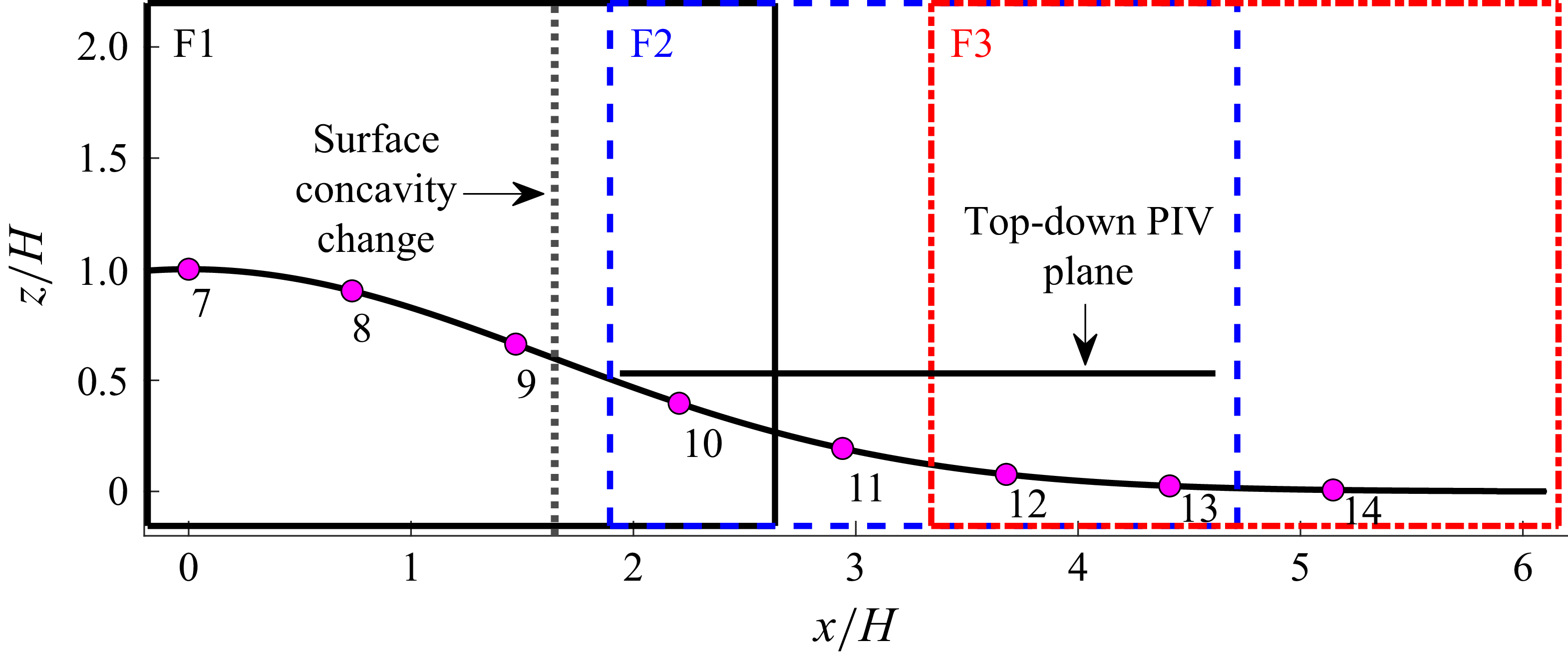
 ⩾20%
 x
 z
 y/H=0,0.75,1.47
 y/H=0
 x/H=1.65
 x
 y
 z/H=0.53

 Cp
 y/H=0
 Cp
 y/H=0
 y/H=±1.47

 x
 z
 x
 z
 y/H=0,0.75,1.47
 x
 y
 z/H=0.53
 y/H=0
 U/U∞
 +
 X
 ∗

 (a)u′2¯
 (b)v′2¯
 (c)u′v′¯
 (d)
 z/H=0.53

 Cp
 4.85×10⁶
 (Δf=0.119Hz,ΔStH=2.0×10⁻⁴)
 (Δf=0.954Hz,ΔStH=1.6×10⁻³)

 y/H=0

 u
 w
 a(1−3)
 a~(1−3)
 10−1

 a(1)

 ΦA(1−3)
 ΦS(1−3)
 ωz

 0.17±0.04
 −0.57±0.08

 aA(1)
 aS(1−3)
 (aA(1),aS(i))

 k
 U+ΦA/S(k)aA/S(k)
 U+ΦA(1)aA(1)+∑i=13ΦS(i)aS(i)
 ωz
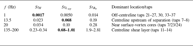
 U∞

 u′2¯
 w′2¯
 x
 z
 y/H=0,0.73,1.47

 u′w′¯
 u′w′¯
 −u′w′¯(∂U/∂z+∂W/∂x)


 Open access

