Introduction
Surface topographical undulations on ice shelves may fill to become meltwater features (mainly lakes and crevasses, although both forms are referred to as ‘meltwater lakes’ hereafter) during the melt season (Glasser & Scambos Reference Glasser and Scambos2008, MacAyeal & Sergienko Reference MacAyeal and Sergienko2013, Luckman et al. Reference Luckman, Elvidge, Jansen, Kulessa, Munneke, King and Barrand2014). They are thought to form as a result of grounding-line flexure (Walker et al. Reference Walker, Parizek, Alley, Anandakrishnan, Riverman and Christianson2013), basal crevassing and channelling (Luckman et al. Reference Luckman, Jansen, Kulessa, King, Sammonds and Benn2012, McGrath et al. Reference McGrath, Steffen, Rajaram, Scambos, Abdalati and Rignot2012, Le Brocq et al. Reference Le Brocq, Ross, Griggs, Bingham, Corr, Ferraccioli, Jenkins, Jordan, Payne, Rippin and Siegert2013), bending at the ice front resulting in surface fractures parallel to the ice front (Scambos et al. Reference Scambos, Fricker, Liu, Bohlander, Fastook, Sargent, Massom and Wu2009), or as a result of incomplete rebound to the previous un-flexed state after lake/crevasse drainage (MacAyeal et al. Reference MacAyeal, Sergienko and Banwell2015). Supraglacial meltwater lakes on ice shelves are, therefore, fundamentally different from lakes on the Greenland ice sheet because they are not controlled by bedrock topography, but are instead able to move with ice flow (Sergienko Reference Sergienko2013, Banwell et al. Reference Banwell, Caballero, Arnold, Glasser, Mac Cathles and MacAyeal2014).
Although treatments of ice-shelf flexure using pure-elastic (Sergienko Reference Sergienko2010, Sayag & Worster Reference Sayag and Worster2011, Banwell et al. Reference Banwell, MacAyeal and Sergienko2013) or viscous (Collins & McCrae Reference Collins and McCrae1985, Ribe Reference Ribe2003, LaBarbera & MacAyeal Reference LaBarbera and MacAyeal2011, Borstad et al. Reference Borstad, Khazendar, Larour, Morlighem, Rignot, Schodlok and Seroussi2012) rheology are common in glaciology, viscoelasticity, especially that which uses Glen’s flow law (i.e. the popular non-linear creep law in glaciology), is rarely used. If the timescale of the phenomena of interest is short, an elastic flexure treatment is justified, whereas if the timescale is very long, a viscous flexure treatment is acceptable. However, as meltwater lakes on ice shelves are thought to fill very slowly over the course of one or more melt seasons, but then drain very quickly in the order of a few hours (Banwell et al. Reference Banwell, MacAyeal and Sergienko2013, MacAyeal & Sergienko Reference MacAyeal and Sergienko2013, MacAyeal et al. Reference MacAyeal, Sergienko and Banwell2015), it is necessary to consider the middle ground of timescales, and this necessitates application of a viscoelastic treatment of ice-shelf flexure.
Our interest in the viscoelastic flexural response of ice shelves to supraglacial lake filling and drainage is strongly motivated by a specific hypothesis that explains a process which probably contributed to the dramatic break-up of the Larsen B Ice Shelf in 2002 (Scambos et al. Reference Scambos, Hulbe and Fahnestock2003, Shepherd et al. Reference Shepherd, Wingham, Payne and Skvarca2003). During the melt season leading up to the collapse of the ice shelf, many supraglacial meltwater lakes were observed to fill (or to remain filled after a previous year’s melt season), and then suddenly drain during the days immediately prior to the initiation of ice-shelf break-up (Glasser & Scambos Reference Glasser and Scambos2008). While meltwater-driven ‘hydrofracture’, the process by which water-filled surface crevasses propagate downwards (van der Veen Reference Van der Veen1998), is certainly a process that contributed to the break-up (Scambos et al. Reference Scambos, Hulbe, Fahnestock and Bohlander2000, Reference Scambos, Fricker, Liu, Bohlander, Fastook, Sargent, Massom and Wu2009, van den Broeke Reference Van den Broeke2005), Banwell et al. (Reference Banwell, MacAyeal and Sergienko2013) have proposed an additional, more macroscopic process that is associated with the filling and draining of supraglacial lakes. Specifically, the temporal change of the gravitational load of a supraglacial lake during filling or draining creates flexure stresses in the ice shelf capable of inducing both surface and basal fractures, both locally and at a distance beyond the lake boundary. This macroscopic behaviour of ice-shelf flexure supports additional meltwater-driven hydrofracture by seeding the ice shelf with a greater density of surface and basal fractures. This behaviour also potentially offers an explanation of why fracture spacing was sufficiently small (Burton et al. Reference Burton, Amundson, Abbot, Boghosian, Cathles, Correa-Legisos, Darnell, Guttenberg, Holland and MacAyeal2012) to support large-scale capsize-driven break-up of the Larsen B Ice Shelf (MacAyeal et al. Reference MacAyeal, Scambos, Hulbe and Fahnestock2003, Banwell et al. Reference Banwell, MacAyeal and Sergienko2013).
Under a purely elastic treatment of ice-shelf flexure (as used by Banwell et al. (Reference Banwell, MacAyeal and Sergienko2013) to model the break-up of the Larsen B Ice Shelf), the filling of a supraglacial lake produces a flexure stress only when it contains meltwater; when it drains, the flexure stress reduces to zero. However, if a viscoelastic treatment is applied (MacAyeal et al. Reference MacAyeal, Sergienko and Banwell2015), flexure stresses that are initially equal to the equivalent pure-elastic stress, decay over time after a supraglacial lake fills. This is because the lake load is supported more and more by the buoyancy of the seawater on the deflected ice-shelf bottom until, eventually, hydrostatic equilibrium may be reached. However, if the lake catastrophically drains before this time, hydrostatic rebound followed by gradual viscoelastic relaxation occurs. Therefore, if drainage does occur, the resultant lake basin at the beginning of the following melt season is likely to be deeper than it was in the previous year. This is both a result of i) incomplete viscoelastic rebound (as excess buoyancy is reduced) to the initial un-flexed ice-shelf surface position after a sudden lake drainage event (MacAyeal et al. Reference MacAyeal, Sergienko and Banwell2015), and ii) enhanced lake-bottom ablation as lake water has a lower albedo compared to the surrounding bare ice (Tedesco et al. Reference Tedesco, Luthje, Steffen, Steiner, Fettweiss, Willis, Bayou and Banwell2012).
In the present study, we apply a treatment of viscoelastic flexure of ice shelves (MacAyeal et al. Reference MacAyeal, Sergienko and Banwell2015) to the problem of the flexural response of an idealized supraglacial lake to annual fill/drain cycles. We hypothesized that, although supraglacial lakes on ice shelves may be too shallow during the first year or two of their existence to cause ice-shelf fracture upon filling/drainage, over multiple years they will deepen and, therefore, evolve towards conditions that allow the possibility of ice-shelf fracture. Our aim is thus to explore the timescale (i.e. the number of seasonal cycles) on which fill/drain cycles enable a lake to reach a ‘critical depth’ such that, upon filling or drainage, the resultant stress may initiate fractures that will subsequently propagate upwards/downwards to become through-cutting crevasses.
Methods
Thin-shelf treatment of viscoelastic ice-shelf flexure
The viscoelastic flexure of an ice shelf was explored using a numerical model that has been implemented in COMSOL (version 4.4). The model predicts the vertical displacement of the ice shelf’s neutral plane, in response to a time-dependent surface load, by evaluating the mechanical balance between the load and forces associated with bending moments and the displacement of seawater. As our aim is to simulate multiple years of evolution of an idealized lake on an ice shelf without having to deal with excessive complexity, azimuthal symmetry is assumed, and so we also used polar co-ordinates r and θ, with the origin, r=0, placed at the lake centre.
The variable η(r,t) describes the vertical displacement of a material surface within the ice shelf that is initially a horizontal plane located halfway between the ice-shelf surface and base. As the ice shelf is loaded by meltwater, and unloaded by drainage and lake-bottom ablation, η(r,t) will become increasingly distorted to account for bending moments and buoyancy forces necessary to balance the changing surface load. As time elapses, the material surface where η=0 will no longer be located halfway between the ice-shelf surface and base. We assume that η≪H, where H is the initial ice thickness, and that changes in ice thickness due to spatially non-uniform ablation are also much less than the initial ice thickness.
Under the above assumptions, our model uses a ‘thin-plate’ approximation to reduce the full 3-D development of viscoelasticity to a much more computationally efficient 2-D form. The model further approximates the elastic and viscous rheological parameters using a constant ice-shelf thickness. (Feedback between changing thickness and changing viscoelastic rheology can be pursued in future studies.) Therefore, the model used in this study is valid primarily where deformations are small (i.e. where vertical deflections are much less than several metres). A more complex, full-Stokes treatment of the problem is possible following the methods applied in other contexts by Gudmundsson (Reference Gudmundsson2011) and by Rosier et al. (Reference Rosier, Gudmundsson and Green2014).
Our approach uses the Maxwell model (Maxwell Reference Maxwell1867) which, represented by a spring and dashpot in series (see MacAyeal et al. Reference MacAyeal, Sergienko and Banwell2015, fig. 1), is useful when elastic deformation and stress are the immediate response to a change in loading and a slow relaxation of the stress accompanied by viscous or creep deformation continues over a long timescale afterwards (Gudmundsson Reference Gudmundsson2011, Rosier et al. Reference Rosier, Gudmundsson and Green2014). This thin-shelf treatment of viscoelastic flexure would usually be justified for situations in which the elastic and viscous parameters are homogeneous. However, in reality, the creep deformation of ice, according to Glen’s flow law, is a non-linear function of stress, whereas the elastic deformation of ice is a linear function of stress. These two functional variations of deformation with stress present an incompatibility between the assumptions commonly used to deal with thin plates and shallow ice shelves. Therefore, following MacAyeal et al. (Reference MacAyeal, Sergienko and Banwell2015), we assume that stresses relevant to determining the curvature of the plate deformation and bending moments are still linear with the vertical co-ordinate inside the ice shelf. This allows us to use an effective viscosity to approximate the creep deformation in response to the initial elastic stress. A description of the model is provided by MacAyeal et al. (Reference MacAyeal, Sergienko and Banwell2015) and is summarized in the supplemental material (found at http://dx.doi.org/10.1017/S0954102015000292).
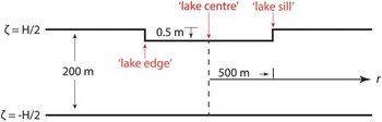
Cross-sectional geometry of the idealized supraglacial lake at t=0 (i.e. before any lake filling occurs). The initial lake basin depth (d) is 0.5 m. The ‘lake edge’ is the point on the lake bottom at r=500 m, and the ‘lake sill’ is the point on the ice-shelf surface at r=500 m, directly above the lake edge. ζ is the vertical distance from the central, neutral plane of the ice shelf. No-displacement, no-bending moment boundary conditions are applied at r=5 km.

Model domain
The ice thickness, H, is taken to be 200 m, comparable to the thickness of the Larsen B Ice Shelf immediately prior to its collapse. No-displacement, no-bending moment boundary conditions are applied at r=5 km (the edge of the ice shelf). We experimented with moving this boundary out to r=10 km (e.g. MacAyeal et al. Reference MacAyeal, Sergienko and Banwell2015), but this had only a negligible effect on results.
The single idealized lake has a circular basin of radius (R) 500 m, and this cannot change throughout the model run. The basin depth (d) is initially 0.5 m at the beginning of the model run, chosen to be just less than the average depth of lakes on the Larsen B Ice Shelf in February 2000 (mean depth=0.8 m, mean maximum depth=1.6 m; Banwell et al. Reference Banwell, Caballero, Arnold, Glasser, Mac Cathles and MacAyeal2014), two years before it catastrophically broke up. The lake geometry is shown in Fig. 1.
Parameters of the simulation are set at arbitrary values representative of ice-shelf conditions: Young’s modulus (E)=10 GPa, Poisson ratio (μ)=0.3, the flow law parameter in Glen’s flow law (n)=3, B=108 Pa s1/3 (corresponding to flow law parameter A=10-24 s-1 Pa-3), sea water density (ρ sw )=1030 kg m-3, and gravitational acceleration at sea level (g)=9.81 m s-2 (MacAyeal et al. Reference MacAyeal, Sergienko and Banwell2015). These parameters are chosen to provide a demonstration that is useful for visualizing the consequences of viscoelastic behaviour; analysis of parameter ranges and sensitivities are relegated to a separate study (if and when the ability to compare model results with observation becomes available).
The behaviour of our simulation is driven by mass loads and deficits. Some loads are periodic and are not conservative (i.e. the lake fills and then drains into the ocean below), and some loads represent permanent changes that are accumulated in the system due to ice/snow ablation. Such loads and deficits are specified in a manner designed to represent typical ice-shelf conditions.
Supraglacial lake fill/drain cycle
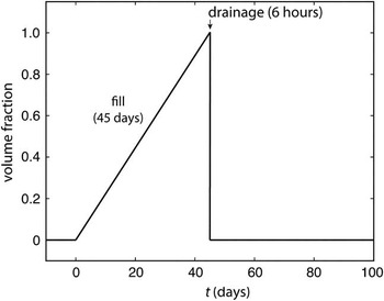
The idealized lake is subjected to a hypothetical fill/drain schedule (non-dimensional units) that applies to one year, and can be repeated sequentially for numbers of years. This is a piecewise continuous function of time which varies from 0 to 1, and back to 0, in order to determine the result of an imposed, non-conservative water source that is available to fill the lake, and then released into the ocean below during drainage. The first 100 days of the fill/drain schedule are shown in Fig. 2. The value of the fill/drain schedule function varies between 0, denoting that the lake basin is entirely empty, to 1, denoting that the lake basin has filled to its maximum water depth (which may or may not be equal to the lake basin depth, depending on whether surface meltwater availability is unlimited or limited – see below for further details). Thus, the rate of water input to the lake during filling, and removal from the lake during drainage, is determined by the volume change (depending on the water depth) needed to change the value of the fill/drain schedule function from 0 to 1. This approach was adopted for simplicity but make note of the complex surface water movement physics that should accompany future study.
Idealized meltwater fill/drain schedule of the supraglacial lake (only the first 100 days of a 365-day schedule are shown). When the volume fraction equals one, the lake has filled to its maximum water depth. The maximum water depth is equal to either i) the elevation of the lake sill for the assumption of unlimited meltwater availability, or ii) 0.8 m for the assumption of limited meltwater availability. Filling is presumed to take 45 days and drainage is presumed to take 6 hours. For 100<t<365 (days), we assume the volume fraction is zero.

The length of the melt season (i.e. the period of time where surface melting, and thus lake filling, occurs) is assumed to be 45 days. This assumption is based on the finding by Scambos et al. (Reference Scambos, Hulbe and Fahnestock2003) that the average melt season length on the Larsen B Ice Shelf was about 45 days from 1979–2000, and also by Leppäranta et al. (Reference Leppäranta, Järvinen and Mattila2013) who reported that supraglacial lakes in the Dronning Maud Land contain liquid water from around 10–20 December until the end of January.
We initially assume that there is an unlimited availability of surface meltwater during each melt season, meaning that the lake can completely fill to its maximum basin depth (i.e. as determined by ice-shelf deflection and lake-bottom ablation). Subsequently, the effect of a limited availability of surface meltwater was investigated, such that lakes can only fill to a maximum water depth of 0.8 m. This depth is chosen as it is equal to the mean measured depth of supraglacial lakes on the Larsen B Ice Shelf on 21 February 2000 (before it broke up in March 2002) (Banwell et al. Reference Banwell, Caballero, Arnold, Glasser, Mac Cathles and MacAyeal2014).
Enhanced lake-bottom ablation is accounted for by assuming a constant rate of 1 cm day-1 throughout the melt season. This rate is significantly lower than observed for supraglacial lakes on the Greenland ice sheet; measured at 6 cm day-1 (and compared to a 2.5–3 cm day-1 ablation rate of bare ice around the lake basin) (Tedesco et al. Reference Tedesco, Luthje, Steffen, Steiner, Fettweiss, Willis, Bayou and Banwell2012). This is because supraglacial lakes on Antarctic ice shelves predominantly consist of slush with varying proportions of ice crystals, at least in Dronning Maud Land (Leppäranta et al. Reference Leppäranta, Järvinen and Mattila2013), and usually have a complete or partial ice-covered surface (Dugan et al. Reference Dugan, Obryk and Doran2013, Leppäranta et al. Reference Leppäranta, Järvinen and Mattila2013, Banwell et al. Reference Banwell, Caballero, Arnold, Glasser, Mac Cathles and MacAyeal2014). The latter feature reduces albedo to 0.2 for ice<10 cm (Ishikawa et al. Reference Ishikawa, Takizawa, Kawamura, Shirasawa and Leppäranta2002) due to the generally negative surface energy balance. The overall effect of lake-bottom ablation is analysed in the Results and Discussion section for the 1-year fill/drain cycle.
Mass loss due to ablation of the ice surface surrounding the lake is not accounted for because we assume that the majority of surface-derived meltwater will percolate downwards into the firn and refreeze (Ligtenberg et al. Reference Ligtenberg, Munneke and van den Broeke2014, Munneke et al. Reference Munneke, Ligtenberg, van den Broeke and Vaughan2014). However, any surface melt that does not refreeze (and is therefore lost to the ocean) will probably be cancelled by the relatively low surface mass gain due to snow accumulation in winter, which, for simplicity, is disregarded.
At the end of the prescribed 45-day melt season, we assume that the lake is drained completely of its water during the first 6 hours of day 46 (Fig. 2), and this is represented by the fill/drain schedule function changing from 1 to 0 over a 6-hour period. In addition to the drainage of the non-conservative meltwater load, lake-bottom ablation means that a fraction of the ice-shelf thickness (specifically 45 cm, if lake-bottom ablation=1 cm day-1) is permanently lost into the ocean as conservative meltwater. This means that, at the point of drainage, the ice shelf is not only losing the load that had become emplaced in the lake during filling, but also the additional load represented by ice originally at the bottom of the lake being melted and lost during the drainage.
Various forms of evidence suggest that the assumption that lake drainage is rapid compared to lake filling is appropriate. For example, sediment cores retrieved from beneath both the former Larsen A and Prince Gustav ice shelves record spatially discrete sediment pulses, interpreted as the drainage of supraglacial lakes and/or crevasses containing sediment, prior to the ice-shelf disintegration event (Gilbert & Domack Reference Gilbert and Domack2003). Additionally, observations of old shorelines and stranded ice blocks on the George VI Ice Shelf indicate catastrophic decreases in water level, often of the order of ~5 m (Reynolds Reference Reynolds1981). Although records of precise timescales of rapid lake drainage events on Antarctic ice shelves are lacking, our 6-hour drainage schedule is motivated by observations of rapid supraglacial lake drainage in Greenland (Tedesco et al. Reference Tedesco, Willis, Hoffman, Banwell, Alexander and Arnold2013).
Stress criterion for fracture initiation
As our aim is to explore the timescale on which fill/drain cycles enable a lake to reach a ‘critical depth’, such that, upon filling or drainage, the resultant stress may initiate fractures in the surrounding ice shelf, we need to select a critical stress value for fracture initiation. Albrecht & Levermann (Reference Albrecht and Levermann2012) found that modelled fracture density using a von Mises (T VM ) stress criterion of 70 kPa compared well with satellite image interpretations of crevasses by Glasser & Scambos (Reference Glasser and Scambos2008, fig. 4) for the Larsen B Ice Shelf. Following the methods of Banwell et al. (Reference Banwell, MacAyeal and Sergienko2013) we also used T VM =70 kPa as our fracture criterion. We do, however, exercise caution when suggesting this value as we are aware that the tensile strength of glacier ice, or even firn, can be much higher than 70 kPa, and the strength of seasonal snow can even reach 70 kPa (Schulson & Duval Reference Schulson and Duval2009). However, given the assumption that any ice shelf will probably have many pre-existing weaknesses and starter cracks with an average length and density (i.e. ‘damage’), we suggest that this stress criterion for fracture initiation is a reasonable one and use it for the remainder of this study.
Simulation set-up
Four simulations were conducted to explore the behaviour of the system. First, we analyse the results of a simulation where the idealized lake (Fig. 1) is subjected to a 1-year fill/drain cycle (Fig. 2) under the assumptions that there is an unlimited availability of meltwater on the ice-shelf surface and that lake-bottom ablation does not occur (Simulation 1). These results were then compared to an identical simulation with the exception that it accounts for lake-bottom ablation (Simulation 2).
The results of a 10-year simulation were then analysed, consisting of annual fill/drain cycles under the assumptions that lake-bottom ablation always occurs and that there is an unlimited availability of surface meltwater (Simulation 3). The results of this simulation were then compared to one that is identical except that it assumes only a limited availability of surface meltwater such that lakes can only fill to a maximum water depth (wd) of 0.8 m (Simulation 4).
The following are the key variables that are explored here.
Vertical displacement, η(r,t)–Vertical displacement of the ice shelf from the original neutral surface of the ice shelf. This responds to both bending moments and to changes in buoyancy. This variable is positive for upward displacement, and negative for downward displacement.
Lake-bottom ablation, ab(t)–Lake-bottom ablation is only active during the melt season, and occurs at a constant rate of 1 cm day-1 over the entire lake bottom. This is set to zero at the beginning of each melt season and is always positive, except in Simulation 1, where it is set to zero.
Net lake-bottom ablation, net_ab(t)–Net lake-bottom ablation is the accumulative value of ab(t) since t=0 days of year 1.
Lake basin depth, d(t)=0.5 m (initial basin depth)+net_ab(t)–(η(lake sill)-η(lake centre))–Lake basin depth is simplified as it ignores the actual geometry of the basin caused by the non-zero η, and instead uses the vertical displacement at two reference points: the lake centre, η(r=0), and the lake sill, η(r=500 m) (for locations see Fig. 1). Lake basin depth is always positive.
Ice-shelf surface profile, s(r,t)=η(r,t)-d(t)–Ice-shelf surface profile is the material surface of the ice, accounting for lake-bottom ablation. It acts to closely represent how the ice-shelf surface elevation would appear.
Water depth, wd(t)≤d(t)–Water depth is assumed to be equal to or less than the lake basin depth (d), depending on whether there is unlimited surface meltwater availability, or a limited surface meltwater availability allowing a maximum water depth of 0.8 m.
Results and discussion
One-year fill/drain cycle: vertical displacement
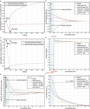
Regardless of whether lake-bottom ablation is included in our simulations, there is no vertical displacement (i.e. η(r=0) is zero) at t=0, indicating the rest position of the ice shelf (Fig. 3a). As the lake reaches full capacity after 45 days of filling, the ice shelf is depressed to just over 0.08 m at the lake centre. If the lake were to remain full, this depression would continue to increase, as the viscoelastic adjustment to the increasing lake load is slow compared to the 45-day filling timescale. However, during day 46 of the simulation, the lake is drained during the initial 6 hours. The following analysis describes the vertical displacement over the remainder of the year, while considering the two assumptions, where: i) lake-bottom ablation does not occur (Simulation 1) and ii) lake-bottom ablation does occur (Simulation 2).
Results of Simulations 1 and 2 for a 1-year fill/drain cycle (Fig. 2) of the idealized supraglacial lake (Fig. 1). a. Vertical displacement, η (m), at the lake centre (r=0) as a function of time, t, assuming that lake-bottom ablation does occur (green line) and that lake-bottom ablation does not occur (red line). b. Vertical displacement, η (m), of the ice shelf, as a function of r, assuming that lake-bottom ablation does occur. c. Basin depth, d (m), as a function of t, assuming that lake-bottom ablation does occur (green line) and that lake-bottom ablation does not occur (red line). Although d is actually positive, it is plotted as a negative number for visualization purposes. d. Ice-shelf surface profile (m), as a function of r, on various days of the year. The initial basin depth at t=0 is 0.5 m. e. Radial (T rr , solid lines) and azimuthal (T θθ , dotted lines) components of the stress as functions of r, at the upper ice surface (ζ=H/2) of the ice shelf on various days during the year. The values of T rr and T θθ at the lower ice surface (ζ=-H/2) are -1 times that shown here. f. Von Mises stress, T VM , as a function of r, evaluated at both the upper and lower surfaces (ζ=±H/2) on various days during the year. The dashed black line indicates the T VM fracture criterion, 70 kPa. The shaded regions in b., d., e. and f. show the lake footprint (r<500 m).

If we assume that the ice shelf behaves purely as an elastic medium and that lake-bottom ablation does not occur (Simulation 1), by the end of the 6-hour drainage event the ice shelf would rebound to its initial, un-flexed position held at t=0. However, as viscoelastic adjustment is able to occur during the 45-day fill period, the ice shelf does not return to its un-flexed position, but instead leaves a depression of ~0.05 m at the end of the sixth hour of day 46 (Fig. 3a). This 0.05 m depression on day 46 accounts for both this viscoelastic adjustment plus the immediate elastic response to the excess buoyancy associated with the ice shelf being depressed by 0.05 m at the end of filling. Following complete drainage, the ice shelf viscoelastically relaxes toward its initial condition prior to lake filling, as the excess buoyancy is reduced. This happens rapidly at first, and then slows. With the parameters used during this simulation, the ice surface does not return to its initial un-flexed state at the end of a 1-year period, but instead an ~0.02 m depression remains at the lake centre.
If, instead, we assume that the ice shelf behaves as an elastic medium, and that lake-bottom ablation does occur (at a rate of 1 cm day-1, Simulation 2), by the end of the 6-hour drainage event, the ice shelf at the lake centre would rebound to its initial, un-flexed position held at t=0, plus an extra ~0.05 m. The additional 0.05 m is due to the immediate elastic response to the excess buoyancy associated with the 0.45 m loss of ice in the lake bottom over the melt season. However, as viscoelastic adjustment occurs during the 45-day fill period, the ice shelf at the lake centre does not rise up as far as this, but instead only rises up by ~0.02 m at the end of the sixth hour of day 46 (Fig. 3a). From day 46 until the end of the year, the ice shelf viscoelastically relaxes towards and beyond its initial vertical displacement prior to lake filling, as the excess buoyancy is reduced. At the end of year 1, the ice surface at the lake centre is just over 0.14 m higher than it was before. The vertical displacement of the ice shelf during the year (for the assumption that lake-bottom ablation occurs) is also illustrated in Fig. 3b as a function of r (i.e. rather than just at the lake centre) for specific days.
One-year fill/drain cycle: basin depth
For both cases without and with lake-bottom ablation, the basin depth is initially 0.5 m (Fig. 3c). With inclusion of lake-bottom ablation, the basin depth increases almost linearly to 0.97 m by the end of day 45. However, without lake-bottom ablation, the basin depth increases non-linearly to only ~0.52 m by the end of day 45. During the 6 hours of lake drainage, the basin depth initially rapidly decreases (by ~0.01 m for both situations), then decreases at a slower rate until the end of the year. For the situations with and without lake-bottom ablation, the basin depths at the end of the year are ~0.90 and ~0.51 m, respectively. Compared to the initial basin depth (0.50 m), the depths have therefore increased by ~0.40 m and ~0.01 m for the simulations with and without bottom-lake ablation, respectively.
These results indicate that lake-bottom ablation has a significant effect on increasing lake basin depth. As lake-bottom ablation is a process that almost certainly occurs during the majority of the melt season in reality, at least to some extent, we present hereafter results of simulations that assume that lake-bottom ablation always occurs during the melt season at a rate of 1 cm day-1 (i.e. Simulations 2, 3 and 4).
One-year fill/drain cycle: ice-shelf surface profile
At the beginning of the year (t=0), before the fill/drain cycle commences, s=0 m is the initial, un-flexed surface, with the 0.5 m deep lake basin superimposed upon this (Fig. 3d). After lake filling has finished on day 45, the lake centre reaches its lowest position for the year, s=-1.05 m, while the lake edge (see Fig. 1 for location) reaches its lowest position, s=-1.03 m (Fig. 3d). Simultaneously, the lake sill (see Fig. 1 for location) has been depressed by ~0.07 m at r=500 m. After drainage on day 46, the lake centre and edge both elastically rebound up to s=~-0.93 m. At this time, a slight up-flexed ‘forebulge’ around the lake basin is created, and this reaches a maximum elevation of s=0.03 m (at r ~0.70 km). From the end of day 46 until day 365, viscoelastic relaxation causes the lake bottom to gradually rise up, until the lake centre ultimately reaches s=-0.76 m, and the lake edge ultimately reaches s=-0.80 m. Meanwhile, the lake sill finally reaches an elevation of s=0.10 m, and the forebulge that had previously existed further away from the lake sill has now subsided.
One-year fill/drain cycle: surface stress analysis
As in Banwell et al. (Reference Banwell, MacAyeal and Sergienko2013; fig. 1), during lake filling, tensile (both radial and azimuthal, T rr and T θθ , respectively) stress exists both at the lower surface of the ice shelf (ζ=-H/2), below the lake basin, and also on the upper surface of the ice shelf (ζ=H/2), around the lake basin, associated with the up-flexed forebulge (Fig. 3e). On day 45, after lake filling, tensile stress is greatest on the lower ice-shelf surface directly under the lake, with T rr reaching 60 kPa at the lake centre (r=0 m). Here, the von Mises stress, T VM =√(T rr 2 +T θθ 2 -T rr T θθ ), reaches 64 kPa (Fig. 3f). As this level of stress is just below our 70 kPa fracture criterion, we suggest that fracture initiation during lake filling is unlikely within the lake basin. Outside of the lake basin, an additional zone of high tensile stress exists on the ice-shelf surface during filling, which is where an up-flexed forebulge would probably be observed. However, here, the maximum T rr is only 16 kPa at r=1.6 km (Fig. 3e), and T VM only reaches a maximum of 20 kPa (Fig. 3f) at the same location, thus the 70 kPa fracture criterion is also not reached outside of the lake basin on day 45.
After drainage on day 46, tensile stress is greatest on the upper ice-shelf surface within the lake basin (Fig. 3e) and reaches a maximum T VM of 90 kPa (Fig. 3f). In the region r≤350 m (which is within the lake basin, r≤500 m), T VM is≥70 kPa, and thus may be large enough to cause ice-shelf fracture. Outside of the lake basin, a zone of low tensile stress exists at the lower ice-shelf surface. However, where T rr only reaches a maximum of 8 kPa (r=2.3 km), T VM only reaches 14 kPa, and is much less than the threshold criterion for fracture.
The above analysis indicates that during the lake’s initial year, T VM only approaches or exceeds 70 kPa within an area that is slightly smaller than the footprint of the lake basin, and this only occurs immediately after drainage. Thus, although fracture within the lake basin may cause itself to drain during the 1-year fill/drain cycle, it is not able to promote fracture at a distance from the lake, and therefore, does not have the potential to drain other nearby lakes through a ‘chain reaction’ process (Banwell et al. Reference Banwell, MacAyeal and Sergienko2013). However, as the ice-shelf surface does not completely return to its un-flexed position after a lake’s 1-year fill/drain cycle, greater meltwater loads will be able to be accommodated during successive fill/drain cycles. Therefore, we hypothesize that the surrounding stress field will become higher in magnitude in subsequent years, thus enabling fracture initiation further away from the lake basin. We investigate this in the next sections (Simulations 3 and 4).
Ten annual fill/drain cycles: basin depth
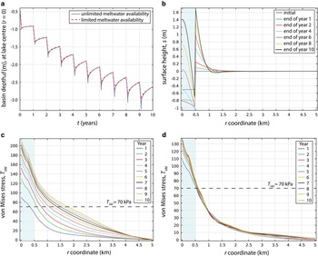
For the assumption of an unlimited availability of meltwater, the final basin depth during year 1 is 0.90 m with maximum d=1.01 m on day 45 (after filling is complete) (Fig. 4a). During year 5, the final basin depth is 1.90 m with maximum d=2.31 m on day 45. During year 10, the final basin depth is 2.64 m with maximum d=3.24 m on day 45. This basin depth is not unreasonable given that water depths of up to ~5 m were measured for the Larsen B Ice Shelf from February 2000 Landsat imagery (Banwell et al. Reference Banwell, Caballero, Arnold, Glasser, Mac Cathles and MacAyeal2014), acquired 2 years prior to the collapse. As the years progress, the difference between the maximum and end-of-year basin depths within each year (i.e. d=0.11 m in year 1, and d=0.60 m in year 10) also increases. This is because the deeper the basin, the larger the volume of water the lake can accommodate, so the greater the difference between the basin depths for the full and drained lake basins.
Results of Simulations 3 and 4 for ten annual fill/drain cycles (Fig. 2) of the idealized supraglacial lake (Fig. 1). a. Basin depth, d (m), assuming unlimited meltwater availability (blue line) and limited meltwater availability (red line). b. Ice-shelf surface profile (m) as a function of r, on various days during the 10 years, under the assumption of unlimited meltwater availability. NB. The plot for the assumption of limited meltwater availability is the same, ±0.02 m. c. Von Mises stress, T VM , as a function of r, evaluated at both the upper and lower surfaces (ζ=±H/2) on day 46 of every year (1–10), for the assumption of unlimited meltwater availability. d. Von Mises stress, T VM , as a function of r, evaluated at both the upper and lower surfaces (ζ=±H/2) on day 46 of every year (1–10), for the assumption of limited meltwater availability. The shaded regions in b., c. and d. show the lake footprint (r<500 m), and the dashed black lines in c. and d. indicate the T VM fracture criterion, 70 kPa.

For the assumption of a limited availability of meltwater (i.e. maximum d=0.8 m), the final basin depth during year 1 is 0.90 m with maximum d=0.99 m on day 45. During year 5, the final basin depth is 1.91 m with maximum d=2.18 m on day 45, and during year 10, the final basin depth is 2.67 m with maximum d=2.30 m on day 45 (Fig. 4a). As for the unlimited meltwater availability assumption, as the years progress, the difference between the maximum and end-of-year basin depths within each year (e.g. equal to 0.08 m in year 1 and 0.32 m in year 10) also increases. However, this occurs more gradually than in the unlimited meltwater availability simulation. We suggest that the reason that the evolution of the basin depth over the 10 years for the two assumptions is similar is related to the strong control that lake-bottom ablation has on basin depth, which occurs at a constant rate independent of water depth.
Ten annual fill/drain cycles: ice-shelf surface profile
At the end of year 1, the lake centre is at s=-0.79 m, the lake edge is at s=-0.81 m and the lake sill is at s=0.10 m (Fig. 3d). Over the following nine years of annual fill/drain cycles, this surface profile generally becomes more exaggerated (Fig. 4b). (NB. Although Fig. 4b is for the assumption of unlimited meltwater availability, the plot for the assumption of limited meltwater availability is equivalent, ±0.02 m.) By the end of year 2, the lake centre reaches its lowest position (s=-0.82 m), while the lake edge is ~0.15 m lower (s=-0.95 m). By the end of year 4, the lake centre is close to its initial position, whereas the lake edge reaches s=-1.05 m; its lowest position over the 10 years. By the end of year 10, the lake centre reaches s=1.42 m, the lake edge reaches s=-0.70 m and the lake sill reaches s=1.70 m (Fig. 4b). An empty, uplifted lake basin such as this is often called a ‘doline’ in analogy to sinkholes in karst terrain (Bindschadler et al. Reference Bindschadler, Scambos, Rott, Skvarka and Vornberger2002, MacAyeal & Sergienko Reference MacAyeal and Sergienko2013).
When the model is run for a further 10 years, the lake centre continues to rise. By the end of year 11, the centre of the lake actually reached a higher elevation than the lake edge, and by the end of year 20, the centre reached an elevation of s=4.2 m (whereas the lake edge only reached s=-0.3 m). This indicates that from year 11 until 20, the lake will probably now be in the form of a ‘moat’ around the (higher) lake centre. MacAyeal & Sergienko (Reference MacAyeal and Sergienko2013, fig. 1) show a photo that may depict such phenomena.
Ten annual fill/drain cycles: surface stress analysis
As our simulations indicate that T VM always reaches its maximum value for the year after drainage on day 46, T VM on day 46 in each of the 10 years, under the assumption of unlimited meltwater availability, is plotted (Fig. 4c). As the years progress, the region where T VM ≥70 kPa increases from r≤0.35 km during year 1, to r≤1.1 km during year 5 and to r≤1.8 km during year 10 (Fig. 4c). Additionally, the maximum T VM at the lake centre increases as the years increase in number, from T VM =90 kPa during year 1 to T VM =180 kPa during year 5 to T VM =214 kPa during year 10.
Thus, the results indicate that, whereas T VM only approaches or exceeds the fracture criterion of 70 kPa within an area slightly smaller than the footprint of the lake basin for a 1-year fill/drain cycle, after multiple annual fill/drain cycles T VM ≥70 kPa over a much larger region that extends beyond the footprint of the lake basin. For example, by the end of year 10, the region r≤1.8 km experiences T VM ≥70 kPa. This means that, although a lake may not be able to promote fracture at a distance during its first fill/drain cycle, it may be able to after multiple years, at which time it may cause other surrounding lakes to drain through a chain reaction process (Banwell et al. Reference Banwell, MacAyeal and Sergienko2013).
However, in contrast to the result above, the equivalent plot of the simulation under the assumption of limited meltwater availability (Fig. 4d) suggests that T VM actually approaches or exceeds the fracture criterion, 70 kPa, within a similar region surrounding the lake for each of the 10 years. This region only varies from where r≤0.53 km on day 46 of year 1 to where r≤0.61 km on day 46 of year 10. These results suggest that, if meltwater is limited, it is unlikely that fracture initiation at a distance from the lake basin will occur. Despite this finding, however, it is likely that some lakes will preferentially fill at the expense of others, perhaps due to small-scale ice-shelf topography, and/or meltwater inflow from nearby overflowing lakes. Therefore, even if the majority of lakes are shallow in depth, if at least one is able to fill to a great enough depth, it may be able to initiate fractures capable of draining other lakes.
Conclusions
We have investigated viscoelastic ice-shelf flexure caused by multiple years of evolution of a single, axisymmetric supraglacial lake on an ice shelf when it is subjected to annual fill/drain cycles. Neither an elastic nor a viscous/creep approach alone would have captured the essential evolution of the flexure process due to: i) the gradual addition of the load (lake filling) resulting in elastic and creep adjustment, and ii) the sudden removal of the load (drainage) resulting in elastic rebound and subsequent gradual viscoelastic relaxation. Although our conclusions are inherently based on the assumption that the lake is able to drain at the end of each melt season, multiple sources of evidence suggest that rapid lake drainage events on ice shelves are frequent and often occur annually.
An a priori assumption was that as the ice-shelf surface does not completely return to its un-flexed position after a lake’s 1-year fill/drain cycle through viscoelastic relaxation, the lake basin is able to deepen over time. Our results indicate that this deepening process is significantly amplified if lake-bottom ablation is assumed to occur. For example, at the end of the 1-year fill/drain cycle, the lake basin experiencing lake-bottom ablation deepened by 40 times more than the amount that the lake basin not experiencing lake-bottom ablation deepened.
We have evaluated the timescale over which the typical lake is able to reach a sufficient depth such that ice-shelf fracture at a distance (i.e. out of the lake basin) is likely to occur in response to lake filling/drainage. We have shown that although this is unlikely to happen during the first year of a lake’s life, after 10 years fracture is possible within a radius of about 2 km from the lake centre. This means that the filling or drainage of one lake may cause surrounding lakes within a radius of a few kilometres to drain through a chain reaction style process. However, this was only true under the assumption that surface meltwater availability was not an overriding limiting factor.
Under the assumption of limited meltwater availability, such that lakes could only fill to a maximum depth equal to the average depth of the lakes on the Larsen B Ice Shelf before it broke up in 2002 (0.8 m), multiple years of annual fill/drain cycles increased the magnitude of the stress field around the lake by a much smaller amount. For this simulation, the region likely to undergo fracture only increased by<100 m radially over the 10 years, producing an area with a radius that was only just larger than the footprint of the lake basin. This suggests that the filling or drainage of one lake is unlikely to cause other lakes to drain if meltwater is limited.
In summary, our results suggest that changing meltwater features on ice shelves (including lakes and water-filled crevasses) produce macroscopically varying stress fields that may cause damage or fracture within a zone extending several kilometres from the features themselves. This process is in addition to the microscopically varying stress fields associated with surface meltwater’s impact on fracture-tip propagation as proposed by previous studies. We suggest that such large-scale stress fields may be as important for fracture as the microscopically varying stress fields associated with hydrofracture, especially with regards to the possibility of triggering chain reaction lake drainage, which, in turn, may lead to large-scale ice-shelf break-up.
Acknowledgements
The authors would like to thank Sebastian Rosier and Hilmar Gudmundsson for help implementing a full-Stokes version of the ice-shelf flexure model with viscoelastic rheology used to check results of the simpler model presented here. Alison Banwell acknowledges the support of an Antarctic Science International Bursary from Antarctic Science Ltd and a Bowring Junior Research Fellowship from St Catharine’s College, Cambridge. We thank Olga Sergienko for valuable modelling assistance and discussions throughout the research. We are grateful to the Editor, Laurie Padman, and to two anonymous reviewers for their valuable comments that helped to improve our initial manuscript.
Author contributions
A.F.B and D.R.M developed the concepts and approach of the study. A.F.B. ran the model, performed the analysis, and wrote the paper. D.R.M. discussed the results and commented on the manuscript.
Supplementary Material
A description of the model will be found at http://dx.doi.org/10.1017/S0954102015000292.