1. Introduction
The law of the wall is a powerful tool for understanding and modelling incompressible wall-bounded turbulent flows (IWBTFs), as it offers a nearly universal description of the mean velocity and temperature profiles within the inner layer. For high Reynolds number IWBTFs with constant fluid properties, the mean streamwise velocity
 $\bar U$
depends solely on the wall shear stress
 $\bar \tau _w$
, wall density
 $\bar \rho _w$
, wall viscosity
 $\bar \mu _w$
, and wall-normal distance
 $Y$
, within the inner layer where
 $Y \ll \varDelta$
, with
 $\varDelta$
denoting the velocity boundary layer thickness (Bradshaw Reference Bradshaw1994; Bradshaw & Huang Reference Bradshaw and Huang1995; Pope Reference Pope2000). Dimensional analysis then yields
 \begin{equation} \bar U^+ = f_U \left ( \frac {\bar \rho _w u_\tau Y}{\bar \mu _w} \equiv Y^+ \right), \end{equation}
where the inner-scaled mean velocity is defined as
 $\bar U^+ = \bar U \!/ u_\tau$
. Here,
 $u_\tau = \sqrt {\bar \tau _w / \bar \rho _w}$
is the friction velocity, and
 $\delta _\nu = \bar \mu _w / (\bar \rho _w u_\tau)$
is the viscous length scale. Hereafter, the subscripts
 $w$
and
 $e$
indicate quantities evaluated at the wall and boundary layer edge, respectively. Equation (1.1) implies that
 $\bar U^+$
can be universally expressed as a function of the inner-scaled wall-normal coordinate
 $Y^+$
. For example, in the viscous sublayer,
 $\bar {U}^+ = Y^+$
, whereas in the logarithmic region,
 $\bar {U}^+ = \ln Y^+ \!/ \kappa + C$
, with
 $\kappa \approx 0.41$
denoting the von Kármán constant, and
 $C \approx 5.2$
as the corresponding intercept (von Kármán Reference von Kármán1930; Prandtl Reference Prandtl1932; Pope Reference Pope2000).
Similarly, the mean temperature difference relative to the wall,
 $\bar {\mathcal{T}}_w - \bar {\mathcal{T}}$
, can be assumed to depend only on the wall shear stress
 $\bar \tau _w$
, wall heat flux
 $\bar q_w$
, wall density
 $\bar \rho _w$
, wall viscosity
 $\bar \mu _w$
, wall thermal conductivity
 $\bar \lambda _w$
, specific heat at constant pressure
 $c_{\!p}$
, and wall distance
 $Y$
, within the inner layer where
 $Y \ll \varDelta$
and
 $Y \ll \varDelta _T$
, with
 $\varDelta _T$
denoting the thermal boundary layer thickness (Kader Reference Kader1991; Bradshaw & Huang Reference Bradshaw and Huang1995). Dimensional analysis then yields
 \begin{equation} \bar {\mathcal{T}}^+ = f_{\mathcal{T}} \left ( \frac {\bar \rho _w u_\tau Y}{\bar \mu _w} \equiv Y^+, \frac {c_{\!p} \bar \mu _w}{\bar \lambda _w} \equiv {\textit{Pr}}_w, \frac {\bar q_w}{\bar \tau _w u_\tau } \equiv \frac {B_q}{(\gamma - 1) M_\tau ^2} \right), \end{equation}
where the inner-scaled mean temperature is given by
 $\bar {\mathcal{T}}^+ = (\bar {\mathcal{T}_w} - \bar {\mathcal{T}}) / T_\tau$
, with
 $T_\tau = \bar q_w / (\bar \rho _w c_{\!p} u_\tau)$
being the friction temperature. Here,
 $B_q = T_\tau / \bar {\mathcal{T}}_w = \bar q_w / (\bar \rho _w u_\tau c_{\!p} \bar {\mathcal{T}}_w)$
is the dimensionless wall heat flux,
 ${\textit{Pr}}_w = c_{\!p} \bar \mu _w / \bar \lambda _w$
is the molecular Prandtl number at the wall, and
 $M_\tau = u_\tau / \sqrt {\gamma R \bar {\mathcal{T}_w}}$
is the friction Mach number. In low-speed flows, the energy dissipation due to friction,
 $\bar \tau _w u_\tau$
, is significantly smaller than the wall heat transfer
 $\bar q_w$
, thus making the dependence on
 $B_q$
negligible. Then
 $f_{\mathcal{T}}$
in (1.2) reduces to a universal function in terms of
 $Y^+$
and
 ${\textit{Pr}}_w$
. For instance, in the conductive sublayer,
 $\bar {\mathcal{T}}^+ = {\textit{Pr}}_w\, Y^+$
, while in the logarithmic region,
 $\bar {\mathcal{T}}^+ = \ln Y^+ \!/ \kappa _T + C_T$
, where the thermal counterpart of the von Kármán constant
 $\kappa _T$
is given by
 $\kappa _T \approx \kappa / {\textit{Pr}}_t \approx 0.48$
(with a constant turbulent Prandtl number
 ${\textit{Pr}}_t \approx 0.85$
there), and the corresponding intercept
 $C_T$
is dependent on
 ${\textit{Pr}}_w$
(Kader Reference Kader1981; Kays & Crawford Reference Kays and Crawford1993). It is interesting to observe that the mean temperature scales similarly to the mean velocity, which is attributed to the Reynolds analogy arising from the decoupling of the momentum and energy equations in low-speed flows (Yang & Abkar Reference Yang and Abkar2018; Chen et al. Reference Chen, Huang, Shi, Yang and Lv2022a
; Huang et al. Reference Huang, Coleman, Spalart and Yang2023; Cheng & Fu Reference Cheng and Fu2024a
).
Unfortunately, these scalings cannot be directly extended to high-speed flows due to the intricate coupling between thermodynamics and hydrodynamics. A widely adopted strategy to address this challenge is to establish a mapping between compressible profiles and their ‘incompressible’ counterparts, accounting for variations in mean flow properties induced by viscous heating (Morkovin Reference Morkovin1962), as well as intrinsic compressibility effects associated with fluid density fluctuations in response to pressure changes (Yu, Xu & Pirozzoli Reference Yu, Xu and Pirozzoli2019; Hasan et al. Reference Hasan, Costa, Larsson, Pirozzoli and Pecnik2025a ). In recent years, considerable efforts have been devoted to developing compressibility transformations for the mean velocity (van Driest Reference Van Driest1951; Zhang et al. Reference Zhang, Bi, Hussain, Li and She2012; Patel, Boersma & Pecnik Reference Patel, Boersma and Pecnik2016; Trettel & Larsson Reference Trettel and Larsson2016; Wu et al. Reference Wu, Bi, Hussain and She2017; Volpiani et al. Reference Volpiani, Iyer, Pirozzoli and Larsson2020; Griffin, Fu & Moin Reference Griffin, Fu and Moin2021b ; Hasan et al. Reference Hasan, Larsson, Pirozzoli and Pecnik2023; Lee et al. Reference Lee, Helm, Martín and Williams2023; Younes & Hickey Reference Younes and Hickey2023; Zhu et al. Reference Zhu, Song, Yang and Xia2024), most of which have been successfully applied to enhance the prediction of mean profiles (Kumar & Larsson Reference Kumar and Larsson2022; Chen et al. Reference Chen, Cheng, Fu and Gan2023; Song, Zhang & Xia Reference Song, Zhang and Xia2023; Hasan et al. Reference Hasan, Larsson, Pirozzoli and Pecnik2024) and to advance near-wall turbulence modelling (Hendrickson et al. Reference Hendrickson, Subbareddy and Candler2022, Reference Hendrickson, Subbareddy, Candler and Macdonald2023; Griffin, Fu & Moin Reference Griffin, Fu and Moin2023; Chen, Gan & Fu Reference Chen, Gan and Fu2024). By contrast, analogous transformations for the mean temperature field have received comparatively limited attention. The earliest notable work appears to be that of Patel, Boersma & Pecnik (Reference Patel, Boersma and Pecnik2017), who proposed van Driest (VD) and Trettel–Larsson (TL) type formulations for variable-property turbulent channel flows in the low-Mach-number limit. These transformations were developed from a series of observed collapse behaviours in the direct numerical simulations (DNS) data, building on and extending their earlier work on mean velocity scalings (Patel et al. Reference Patel, Boersma and Pecnik2016). Subsequently, Wan et al. (Reference Wan, Zhao, Liu, Wang and Lei2020) conducted a similar analysis for channel flows at supercritical pressure, and extended the TL-type transformation. They reported that the transformation effectively accounts for thermophysical property variations in the inner layer, provided that the effects of different local Prandtl numbers are neglected. Chen et al. (Reference Chen, Huang, Shi, Yang and Lv2022a ) further generalised the VD- and TL-type transformations to high-speed flows over isothermal and adiabatic walls by accounting for the combined effects of viscous heating and wall heat transfer on the local total heat flux. Using their self-built DNS database of supersonic Couette flows with various wall thermal boundary conditions, they demonstrated that the corrected TL-type transformation successfully collapses mean temperature profiles across adiabatic, heated and cooled walls, whereas the VD-type transformation fails in cold-wall conditions. However, their transformations rely heavily on DNS inputs. To address this, Huang et al. (Reference Huang, Coleman, Spalart and Yang2023) re-derived the VD- and TL-type temperature transformations directly from the mean total energy equation, in a manner analogous to the derivation of mean velocity scalings. By neglecting the molecular and turbulent diffusion terms of turbulent kinetic energy in the total heat flux equation, they obtained closed-form expressions for both transformations, along with a unified description for isothermal and adiabatic walls. Recently, Cheng & Fu (Reference Cheng and Fu2024a ) thoroughly clarified the impact of the higher-order terms omitted in the derivation, and developed a new temperature transformation inspired by the mean velocity scaling proposed by Younes & Hickey (Reference Younes and Hickey2023). Through systematic comparisons with DNS datasets of canonical compressible wall-bounded turbulent flows (CWBTFs), they demonstrated that the proposed transformation offers significant improvements over the TL-type method, particularly in compressible turbulent channel flows (CTCFs) with adiabatic walls, and zero-pressure-gradient (ZPG) compressible turbulent boundary layer flows (CTBLFs) over cold walls. Most recently, Zhu et al. (Reference Zhu, Zhang, Yang, Ji and Xia2025b ) developed a unified framework for mean temperature transformations in CTCFs by introducing the concept of the mixed Prandtl number, and establishing a connection between the compressible total heat flux equation and its ‘incompressible’ counterpart. While encompassing all existing approaches, the proposed framework enables the formulation of novel temperature transformations through its integration with arbitrary mean velocity scalings. Accordingly, the primary objective of the present study is to generalise this framework to canonical CWBTFs and to develop more accurate temperature transformations by incorporating more advanced, Mach-invariant mean velocity scalings.
In the near-wall region of CWBTFs at high Reynolds numbers and Mach numbers, the presence of steep velocity and temperature gradients demands highly refined grid resolution for accurate capture, thereby inevitably increasing computational costs. To address this challenge, near-wall models within the framework of Reynolds-averaged Navier–Stokes (RANS) and wall-modelled large eddy simulations (WMLES) have been developed to reduce the near-wall resolution requirements and accelerate computations (Chen et al. Reference Chen, Lv, Xu, Shi and Yang2022b ; Griffin et al. Reference Griffin, Fu and Moin2023; Chen et al. Reference Chen, Gan and Fu2024; Cheng et al. Reference Cheng, Chen, Zhu, Shyy and Fu2024). Wall models for mean velocity are typically extensions of the classical incompressible law of the wall to high-speed flows, achieved either by eliminating compressibility effects through velocity transformations, or by re-deriving composite formulations for compressible mean velocity profiles based on the scaling laws of different wall layers (Nichols & Nelson Reference Nichols and Nelson2004; Li et al. Reference Li, Gao, Mo and Jiang2025a ). For modelling mean temperature, previous studies commonly adopt algebraic mean temperature–velocity (TV) relations, which are derived under the assumption of an intrinsic similarity between velocity and temperature fields (Busemann Reference Busemann1931; Crocco Reference Crocco1932; Walz Reference Walz1969; Duan & Martin Reference Duan and Martin2011; Cheng & Fu Reference Cheng and Fu2024b ). Among these, the most widely adopted and effective approach is the generalised Reynolds analogy (GRA) relation developed by Zhang et al. (Reference Zhang, Bi, Hussain and She2014):
 \begin{equation} \frac {\tilde {T}}{\tilde {T}_w}=1+\frac {\tilde {T}_{rg}-\tilde {T}_w}{\tilde {T}_w}\frac {\tilde {u}}{\tilde {u}_e}+\frac {\tilde {T}_e-\tilde {T}_{rg}}{\tilde {T}_w}\left ( \frac {\tilde {u}}{\tilde {u}_e} \right) ^2, \end{equation}
where
 $\tilde {T}_{rg} = \tilde {T}_e + r_g \tilde {u}_e^2 / (2c_{\!p})$
, and the general recovery factor
 $r_g$
is defined as
 $r_g = 2c_{\!p} (\tilde {T}_w - \tilde {T}_e) / \tilde {u}_e^2 + (2c_{\!p} / \tilde {u}_e) \times \partial \tilde {T} \!/ \partial \tilde {u} \big|_w$
. When combined with the perfect gas law, the
 $\bar {\mu }{-}\tilde {T}$
relation, and other well-established relations, the velocity and temperature wall models form a closed system that can be solved iteratively to predict inner layer mean profiles. Despite the demonstrated success of (1.3), evaluating the term
 $\partial \tilde {T} \!/ \partial \tilde {u} \big |_w$
relies on the Reynolds analogy, expressed as
 $s = 2C_h / C_{\!f} = \bar {q}_w \tilde {u}_e / [\bar {\tau }_w c_{\!p} {(\tilde {T}_w - \tilde {T}_r)}]$
, where
 $\tilde {T}_r = \tilde {T}_e + r \tilde {u}_e^2 / (2c_{\!p})$
and
 $r = Pr^{1/3}$
, with
 ${\textit{Pr}} \approx 0.7$
and
 $s \approx 1.14$
for canonical air flows. As a result, the GRA relation inherently depends on boundary-layer-edge quantities
 $\tilde {u}_e$
and
 $\tilde {T}_e$
, even if the boundary conditions are reassessed at a matching location
 $y = y_m$
(Griffin et al. Reference Griffin, Fu and Moin2023; Chen et al. Reference Chen, Gan and Fu2024, Reference Chen, Gan and Fu2025). Such dependence limits the applicability of the corresponding temperature wall model in complex flow configurations, where determining the boundary layer edge is non-trivial (Griffin et al. Reference Griffin, Fu and Moin2021a
). Most recently, Chen, Gan & Fu (Reference Chen, Gan and Fu2025) proposed a novel temperature wall model that eliminates dependence on boundary-layer-edge quantities by coupling the GRA relation with the temperature transformation developed by Cheng & Fu (Reference Cheng and Fu2024a
). While this approach demonstrates high accuracy in ZPG CTBLFs with wall heat transfer, its practical implementation is inconvenient due to the non-monotonic behaviour of the mean temperature profile and the limited accuracy of existing temperature transformations. Accordingly, the secondary objective of the present study is to explore alternative strategies for near-wall temperature modelling, with particular emphasis on addressing the non-monotonic mean temperature distributions in ZPG CTBLFs with cold walls.
With the two aforementioned objectives, the remainder of the paper is organised as follows. In § 2, we rigorously derive the general framework for velocity and temperature transformations, and elucidate their connection to the development of compressible eddy viscosity and eddy thermal conductivity models. The DNS database employed to construct the ‘incompressible’ reference profiles is described in § 3, where the modelling of the mixed Prandtl number is also discussed. A series of novel temperature transformations is proposed and systematically evaluated in § 4, using DNS datasets of canonical CWBTFs covering a broad range of Mach numbers, Reynolds numbers and wall thermal boundary conditions. We also examine the impact of the simplifications made in the derivation, and evaluate the corresponding compressible eddy thermal conductivity models. In § 5, the integral mean TV relation introduced by Zhu et al. (Reference Zhu, Zhang, Yang, Ji and Xia2025b ) is extended, and inverse temperature transformations are presented, with a preliminary exploration of their potential and limitations in near-wall temperature modelling. Finally, concluding remarks are offered in § 6.
2. Derivation of the general framework
2.1. The compressible RANS equations
The Reynolds-averaged governing equations for compressible flows, including the continuity, momentum and total energy equations, are given as (Gatski & Bonnet Reference Gatski and Bonnet2009; Raje et al. Reference Raje, Parish, Hickey, Cinnella and Duraisamy2025)
 \begin{equation} \frac {\partial \bar \rho }{\partial t} + \frac {\partial \bar \rho \tilde u_{\!j}}{\partial x_{\!j}} = 0, \end{equation}
 \begin{equation} \frac {\partial \bar \rho \tilde u_i}{\partial t} + \frac {\partial \bar \rho \tilde u_i \tilde u_{\!j}}{\partial x_{\!j}} = -\frac {\partial \bar p}{\partial x_i} + \frac {\partial }{\partial x_{\!j}} \left ( \bar \tau _{ij} - \bar \rho\, \widetilde {u_i^{\prime \prime }u_{\!j}^{\prime \prime }} \right) + \bar F\delta _{i1}, \end{equation}
 \begin{equation} \frac {\partial \bar \rho \tilde E}{\partial t} + \frac {\partial \bar \rho \tilde E \tilde u_{\!j}}{\partial x_{\!j}} = -\frac {\partial \overline {p u_{\!j}}}{\partial x_{\!j}} + \frac {\partial \overline {\tau _{ij} u_i}}{\partial x_{\!j}} + \frac {\partial }{\partial x_{\!j}} \left ( \overline {\lambda \frac {\partial T}{\partial x_{\!j}}} - \bar \rho\, \widetilde {E^{\prime \prime }u_{\!j}^{\prime \prime }} \right) + \overline {\textit{Fu}_1}. \end{equation}
Here,
 $i = 1, 2, 3$
correspond to the streamwise (
 $x$
), wall-normal (
 $y$
) and spanwise (
 $z$
) directions, respectively, and
 $\delta _{ij}$
is the Kronecker delta. The flow variables are defined as follows:
 $u_i$
is the
 $i$
th velocity component, and
 $\rho$
,
 $p$
and
 $T$
are the density, pressure and temperature, respectively. The viscous stress tensor is given by
 $\tau _{ij}=\mu (\partial u_i/\partial x_j+\partial u_j/\partial x_i-(2/3)(\partial u_k/\partial x_k)\delta _{ij})$
,
 $F$
denotes the streamwise body force (
 $F = 0$
in ZPG CTBLFs), and
 $E = c_v T + u_i u_i / 2$
is the total energy per unit mass, where
 $c_v = c_{\!p} / \gamma = R / (\gamma - 1)$
is the specific heat at constant volume,
 $\gamma$
is the specific heat ratio, and
 $R$
is the specific gas constant. Both Reynolds averaging (
 $\bar \varGamma$
) and Favre averaging (
 $\tilde \varGamma =\overline {\rho \varGamma }\!/\!\bar \rho$
) are employed for any flow quantity
 $\varGamma$
, with
 $\varGamma ^{\prime }$
and
 $\varGamma ^{\prime \prime }$
denoting the corresponding fluctuating components, respectively.
In the following, the total shear stress and total heat flux are defined as
 \begin{equation} \bar \tau _t = \bar \mu \frac {\partial \tilde u}{\partial y} - \bar \rho\, \widetilde {u^{\prime \prime }v^{\prime \prime }\ } \quad \text{and} \quad \bar q_t = -\bar \lambda \frac {\partial \tilde T}{\partial y} + c_{\!p} \bar \rho\, \widetilde {T^{\prime \prime }v^{\prime \prime }}. \end{equation}
Two non-dimensionalisation approaches are adopted. The inner scaling is characterised by the wall friction velocity
 $u_\tau = \sqrt {\bar \tau _w / \bar \rho _w}$
, the wall viscous length scale
 $\delta _\nu = \bar \mu _w / (\bar \rho _w u_\tau)$
, and the wall friction temperature
 $T_\tau = \bar q_w / (\bar \rho _w c_{\!p} u_\tau)$
, and is denoted using a superscript ‘+’. The semi-local scaling is defined using the semi-local friction velocity
 $u_\tau ^* = \sqrt {\bar \tau _w / \bar \rho }$
, the semi-local viscous length scale
 $\delta _\nu ^* = \bar \mu / (\bar \rho u_\tau ^*)$
, and the semi-local friction temperature
 $T_\tau ^* = \bar q_w / (\bar \rho c_{\!p} u_\tau ^*)$
, and is indicated by a superscript ‘*’.
2.2. Velocity transformations and compressible eddy viscosity models
For CWBTFs, the total shear stress equation (2.4) can be expressed in non-dimensional form by normalising with the wall shear stress
 $\bar \tau _w$
:
 \begin{equation} \left ( \frac {\partial \tilde u}{\partial y} \right)^* - \widetilde {u^{\prime \prime }v^{\prime \prime }\ }^* = \bar \tau _{t,{\textit{com}}}^+, \end{equation}
where
 $(\partial \tilde u / \partial y)^* = (\partial \tilde u / \partial y) / (u_\tau ^* \,/ \delta _\nu ^*) = \bar \mu ^+\, \partial \tilde u^+ \!/ \partial y^+$
represents the viscous shear stress, with
 $\tilde u^+ = \tilde u / u_\tau$
. The term
 $-\widetilde {u^{\prime \prime }v^{\prime \prime }\ }^* = -\widetilde {u^{\prime \prime }v^{\prime \prime }\ } / u_\tau ^{*2} = -\bar \rho\, \widetilde {u^{\prime \prime }v^{\prime \prime }\ } / (\bar \rho _w u_\tau ^2) = -\bar \rho ^+\, \widetilde {u^{\prime \prime }v^{\prime \prime }\ }^+$
denotes the turbulent shear stress, and
 $\bar \tau _{t,{\textit{com}}}^+ = \bar \tau _{t,{\textit{com}}} / \bar \tau _w$
is the total shear stress. Here,
 $\bar \mu ^+ = \bar \mu / \bar \mu _w$
and
 $\bar \rho ^+ = \bar \rho / \bar \rho _w$
denote the inner-scaled mean viscosity and density, respectively. Throughout this paper, the subscripts ‘
 $com$
’ and ‘
 $in$
’ refer to compressible and ‘incompressible’ states, respectively.
The total shear stress equation for the corresponding ‘incompressible’ state is given by
 \begin{equation} \left ( \frac {\partial \bar U}{\partial Y} \right)^+ - \overline {U^{\prime }V^{\prime }}^+ = \bar \tau _{t,{\textit{in}}}^+, \end{equation}
where the ‘incompressible’ viscous shear stress is defined as
 $(\partial \bar U \!/ \partial Y)^+ = (\partial \bar U \!/ \partial Y) / (u_\tau / \delta _\nu) = \partial \bar U^+ \!/ \partial Y^+$
, with
 $\bar U^+ = \bar U \!/ u_\tau$
, and the turbulent shear stress is
 $-\overline {U^{\prime }V^{\prime }}^+ = -\overline {U^{\prime }V^{\prime }} / u_\tau ^2$
. The ‘incompressible’ total shear stress is denoted as
 $\bar \tau _{t,{\textit{in}}}^+ = \bar \tau _{t,{\textit{in}}} / \bar \tau _w$
. Here,
 $U$
,
 $V$
and
 $Y$
represent the transformed ‘incompressible’ streamwise velocity, wall-normal velocity and wall-normal distance, respectively.
It can be observed that the introduction of semi-local scaling leads to a similar form of the total shear stress equations for both compressible and ‘incompressible’ states. To further simplify the expressions, we define the compressible and ‘incompressible’ eddy viscosities as
 $\bar \mu _{t,{\textit{com}}} / \bar \mu = -\widetilde {u^{\prime \prime }v^{\prime \prime }\ }^* \!/ (\partial \tilde u / \partial y)^*$
and
 $\bar \mu _{t,{\textit{in}}} / \bar \mu _w = -\overline {U^{\prime }V^{\prime }}^+ \!/ (\partial \bar U \!/ \partial Y)^+$
, respectively. Then (2.5) and (2.6) can be rewritten as
 \begin{equation} \left ( 1 + \frac {\bar \mu _{t,{\textit{com}}}}{\bar \mu } \right) \left ( \frac {\partial \tilde u}{\partial y} \right)^* = \bar \tau _{t,{\textit{com}}}^+, \end{equation}
 \begin{equation} \left ( 1 + \frac {\bar \mu _{t,{\textit{in}}}}{\bar \mu _w} \right) \left ( \frac {\partial \bar U}{\partial Y} \right)^+ = \bar \tau _{t,{\textit{in}}}^+. \end{equation}
As noted, the semi-local scaling renders the compressible mean momentum equation structurally similar to its ‘incompressible’ counterpart, which indirectly supports its validity for extending incompressible models to high-speed flows. Dividing (2.8) by (2.7) then leads to a general framework for mean velocity transformations, given by
 \begin{equation} \bar U^+ = \int _{0}^{\tilde u^+}{\frac {\bar \tau _{t,{\textit{in}}}^+}{\bar \tau _{t,{\textit{com}}}^+} \frac {1 + \bar \mu _{t,{\textit{com}}} / \bar \mu }{1 + \bar \mu _{t,{\textit{in}}} / \bar \mu _w}\, \bar \mu ^+\, \frac {{\partial } Y^+}{{\partial } y^+}\, \mathrm{d}\tilde u^+}. \end{equation}
It should be noted that an expression similar to (2.9) was first proposed by Hasan et al. (Reference Hasan, Larsson, Pirozzoli and Pecnik2023) for CWBTFs. However, the authors neglected the differences in total shear stresses before and after the transformation. A comparable framework, based on the mixing length concept, was introduced by Zhu et al. (Reference Zhu, Song, Yang and Xia2024). In fact, all transformations must satisfy (2.9), and we mainly consider six transformations in this paper: TL (Patel et al. Reference Patel, Boersma and Pecnik2016; Trettel & Larsson Reference Trettel and Larsson2016), GFM (Griffin et al. Reference Griffin, Fu and Moin2021b ), HLPP (Hasan et al. Reference Hasan, Larsson, Pirozzoli and Pecnik2023), ZSYX (Zhu et al. Reference Zhu, Song, Yang and Xia2024), SLVD (the semi-local van Driest transformation for the logarithmic layer, proposed by Younes & Hickey Reference Younes and Hickey2023), and VIPL (Volpiani et al. Reference Volpiani, Iyer, Pirozzoli and Larsson2020) transformations, as detailed in Appendix A.
On the one hand, (2.9) can be directly employed to develop new velocity transformations, provided that the Mach-invariance of eddy viscosity under a certain transformed coordinate
 $Y^+$
is assumed and validated, i.e.
 \begin{equation} \bar \mu _{t,{\textit{com}}} / \bar \mu = \bar \mu _{t,{\textit{in}}} / \bar \mu _w = f\!(Y^+, {\textit{Re}}_T), \end{equation}
where
 $f\!(Y^+, {\textit{Re}}_T)$
is a universal function describing the ‘incompressible’ eddy viscosity profile with respect to the inner coordinate
 $Y^+$
, parametrised by the friction Reynolds number
 ${\textit{Re}}_T$
. For instance, in the inner layer of high Reynolds number IWBTFs, it is typically adopted as
 $f\!(Y^+, {\textit{Re}}_T) = \kappa Y^+ [1 - \exp(-Y^+ \!/ A^+) ]^2$
, where
 $\kappa = 0.41$
and
 $A^+ = 17$
(Johnson & King Reference Johnson and King1985). The original TL and VIPL transformations, given in (A1) and (A6), serve as representative examples. They can be derived by substituting the transformed coordinates
 $Y^+ = y^*$
and
 $Y^+ = y_V^+$
into (2.10), while further neglecting the differences in total shear stresses before and after transformation, i.e.
 $\bar \tau _{t,{\textit{com}}}^+ = \bar \tau _{t,{\textit{in}}}^+$
, which was originally motivated by the constant-stress layer assumption (Trettel & Larsson Reference Trettel and Larsson2016; Volpiani et al. Reference Volpiani, Iyer, Pirozzoli and Larsson2020).
On the other hand, (2.9) can also be used to develop compressible eddy viscosity models by incorporating advanced mean velocity scalings (Yang & Lv Reference Yang and Lv2018; Hendrickson et al. Reference Hendrickson, Subbareddy and Candler2022, Reference Hendrickson, Subbareddy, Candler and Macdonald2023; Chen et al. Reference Chen, Gan and Fu2024), which may be derived through various approaches. For clarity and convenience, we first introduce the modified TL and VIPL transformations,
 \begin{equation} \bar U_{{\textit{TL}},m}^+ = \int _{0}^{\bar U_{\textit{TL}}^+}{\frac {\bar \tau _{t,{\textit{in}}}^+}{\bar \tau _{t,{\textit{com}}}^+}\, \mathrm{d}\bar U_{\textit{TL}}^+} \quad \text{and} \quad \bar U_{\textit{VIPL},m}^+ = \int _{0}^{\bar U_{\textit{VIPL}}^+}{\frac {\bar \tau _{t,{\textit{in}}}^+}{\bar \tau _{t,{\textit{com}}}^+}\, \mathrm{d}\bar U_{\textit{VIPL}}^+}, \end{equation}
which extend the original formulations (A1) and (A6) by additionally accounting for differences in
 $\bar \tau _{t,{\textit{com}}}^+$
and
 $\bar \tau _{t,{\textit{in}}}^+$
. As presented in Appendix A, the TL, GFM, HLPP, ZSYX and SLVD transformations all acknowledge the semi-local transformed coordinate
 $Y^+ = y^*$
, implying a consistent form of the ‘incompressible’ eddy viscosity,
 $\bar \mu _{t,{\textit{in}}} / \bar \mu _w = f\!(y^*, {\textit{Re}}_{\tau ,e}^*)$
. Based on (2.9), these mean velocity scalings can thus be interpreted as different modelling approaches for the compressible eddy viscosity
 $\bar \mu _{t,{\textit{com}}} / \bar \mu$
. Substituting
 $Y^+ = y^*$
into (2.9) and combining with the modified TL transformation in (2.11), the compressible eddy viscosity corresponding to any
 $y^*$
-based transformation
 $\bar U_{\textit{trans}}^+ (y^*)$
can be expressed as
 \begin{equation} 1 + \left ( \frac {\bar \mu _{t,{\textit{com}}}}{\bar \mu } \right)_{\textit{model}} = \frac {\partial \bar U_{\textit{trans}}^+ / \partial \tilde u^+}{\partial \bar U_{{\textit{TL}},m}^+ / \partial \tilde u^+} \left [ 1 + f\!(y^*, {\textit{Re}}_{\tau ,e}^*) \right ]. \end{equation}
Equation (2.12) offers physical insight into the extension of incompressible eddy viscosity models to high-speed flows through the inclusion of compressibility effects. Clearly, a more accurate transformation yields a compressible eddy viscosity model
 $(\bar \mu _{t,{\textit{com}}} / \bar \mu)_{\textit{model}}$
that agrees better with compressible DNS data
 $(\bar \mu _{t,{\textit{com}}} / \bar \mu)_{\textit{DNS}}$
. It is noteworthy that (2.12) differs slightly from the formulations proposed in previous studies (Hendrickson et al. Reference Hendrickson, Subbareddy and Candler2022, Reference Hendrickson, Subbareddy, Candler and Macdonald2023; Chen et al. Reference Chen, Gan and Fu2024), where the authors refined the semi-local model implied by the TL transformation using the GFM transformation. Their model can be expressed as
 \begin{equation} \left ( \frac {\bar \mu _{t,{\textit{com}}}}{\bar \mu } \right)_{\textit{model}} = \frac {\partial \bar U_{\textit{GFM}}^+ / \partial \tilde u^+}{\partial \bar U_{\textit{TL}}^+ / \partial \tilde u^+} f\!(y^*, {\textit{Re}}_{\tau ,e}^*). \end{equation}
A detailed examination of their derivation indicates that (2.13) represents a special case of (2.12) within the logarithmic layer, without accounting for the difference between
 $\bar \tau _{t,{\textit{com}}}^+$
and
 $\bar \tau _{t,{\textit{in}}}^+$
. Nevertheless, as the GFM transformation largely retains the TL scaling below the buffer layer, this simplification does not significantly impact the overall model accuracy.
2.3. Temperature transformations and compressible eddy thermal conductivity models
As previously noted by Huang et al. (Reference Huang, Coleman, Spalart and Yang2023) and Modesti & Pirozzoli (Reference Modesti and Pirozzoli2024), the formulation of the mean temperature scalings may proceed in a manner analogous to that used for mean velocity transformations. We begin by considering the case with wall heat transfer, i.e.
 $\bar q_w \neq 0$
. The compressible total heat flux equation in (2.4) is non-dimensionalised using the wall heat flux
 $\bar q_w$
, yielding
 \begin{equation} \frac {1}{Pr} \left ( \frac {\partial \tilde T}{\partial y} \right)^* - \widetilde {T^{\prime \prime }v^{\prime \prime }}^* = \bar q_{t,{\textit{com}}}^+, \end{equation}
where
 ${\textit{Pr}}^{-1}\,(\partial \tilde T \!/ \partial y)^* = - Pr^{-1}\, (\partial \tilde T \!/ \partial y) / (T_\tau ^* \!/ \delta _\nu ^*) = {\textit{Pr}}_w^{-1}\, \bar \lambda ^+\, \partial \tilde T^+ \!/ \partial y^+$
represents the molecular heat flux, with
 $\tilde T^+ = (\tilde T_w - \tilde T) / T_\tau$
denoting the inner-scaled mean temperature. The term
 $-\widetilde {T^{\prime \prime }v^{\prime \prime }}^* = \widetilde {T^{\prime \prime }v^{\prime \prime }} / (T_\tau ^* u_\tau ^*) = \bar \rho\, \widetilde {T^{\prime \prime }v^{\prime \prime }} / (\bar \rho _w T_\tau u_\tau) = -\bar \rho ^+\, \widetilde {T^{\prime \prime }v^{\prime \prime }}^+$
is the turbulent heat flux, and
 $\bar q_{t,{\textit{com}}}^+ = \bar q_{t,{\textit{com}}} / \bar q_w$
the total heat flux. Here,
 $\bar \lambda ^+ = \bar \lambda / \bar \lambda _w$
denotes the inner-scaled mean thermal conductivity, and
 ${\textit{Pr}} = c_{\!p} \bar \mu / \bar \lambda$
is the local molecular Prandtl number.
For the transformed ‘incompressible’ counterpart, the total heat flux equation is given by
 \begin{equation} \frac {1}{{\textit{Pr}}_w} \left ( \frac {\partial \bar {\mathcal{T}}}{\partial Y} \right)^+ - \overline {\mathcal{T}^{\prime }V^{\prime }}^+ = \bar q_{t,{\textit{in}}}^+, \end{equation}
where the ‘incompressible’ molecular heat flux is defined as
 ${\textit{Pr}}_w^{-1}\,(\partial \bar {\mathcal{T}} / \partial Y)^+ = -{\textit{Pr}}_w^{-1}\,(\partial \bar {\mathcal{T}} / \partial Y) / (T_\tau / \delta _\nu) = {\textit{Pr}}_w^{-1}\,\partial \bar {\mathcal{T}}^+ \!/ \partial Y^+$
, with
 $\bar {\mathcal{T}}^+ = (\bar {\mathcal{T}}_w - \bar {\mathcal{T}}) / T_\tau$
, and the turbulent heat flux is
 $-\overline {\mathcal{T}^{\prime }V^{\prime }}^+ = \overline {\mathcal{T}^{\prime }V^{\prime }} / (T_\tau u_\tau)$
. The ‘incompressible’ total heat flux is denoted as
 $\bar q_{t,{\textit{in}}}^+ = \bar q_{t,{\textit{in}}} / \bar q_w$
.
Consistent with the approach in § 2.2, we introduce compressible and ‘incompressible’ eddy thermal conductivities, defined respectively as
 $\bar \lambda _{t,{\textit{com}}} / \bar \lambda = - Pr\, \widetilde {T^{\prime \prime }v^{\prime \prime }}^* \!/ ( {\partial \tilde T} / {\partial y})^*$
and
 $\bar \lambda _{t,{\textit{in}}} / \bar \lambda _w = - {\textit{Pr}}_w\, \overline {\mathcal{T}^{\prime }V^{\prime }}^+ \!/ ( {\partial \bar {\mathcal{T}}} / {\partial Y})^+$
, for further simplifications. Equations (2.14) and (2.15) can then be rewritten as
 \begin{equation} \left ( 1 + \frac {\bar \lambda _{t,{\textit{com}}}}{\bar \lambda } \right) \frac {1}{Pr} \left ( \frac {\partial \tilde T}{\partial y} \right)^* = \bar q_{t,{\textit{com}}}^+, \end{equation}
 \begin{equation} \left ( 1 + \frac {\bar \lambda _{t,{\textit{in}}}}{\bar \lambda _w} \right) \frac {1}{{\textit{Pr}}_w} \left ( \frac {\partial \bar {\mathcal{T}}}{\partial Y} \right)^+ = \bar q_{t,{\textit{in}}}^+. \end{equation}
It is worth noting that (2.16) becomes ill-defined in the presence of adiabatic walls, because
 $\bar q_w = 0$
. To address this issue, we reformulate (2.16) into a more unified expression, following the methodology proposed in previous studies (Chen et al. Reference Chen, Huang, Shi, Yang and Lv2022a
; Huang et al. Reference Huang, Coleman, Spalart and Yang2023; Cheng & Fu Reference Cheng and Fu2024a
):
 \begin{equation} \left ( 1 + \frac {\bar \lambda _{t,{\textit{com}}}}{\bar \lambda } \right) \frac {\bar \lambda ^+}{{\textit{Pr}}_w} \frac {\partial \theta }{\partial y^+} = B_q \bar q_{t,{\textit{com}}}^+, \end{equation}
where
 $\theta = 1 - \tilde T \!/ \tilde T_w$
,
 $B_q = \bar q_w / (\bar \rho _w c_{\!p} u_\tau \tilde T_w)$
and
 $\bar q_{t,{\textit{com}}}^+ = \bar q_{t,{\textit{com}}} / \bar q_w$
. Dividing (2.17) by (2.18) then yields a general framework for the mean temperature transformation, given by
 \begin{equation} \bar {\mathcal{T}}^+ = \int _{0}^{\theta }{\frac {{\textit{Pr}}_w}{Pr} \frac {1 + \bar \lambda _{t,{\textit{com}}} / \bar \lambda }{1 + \bar \lambda _{t,{\textit{in}}} / \bar \lambda _w} \frac {\bar q_{t,{\textit{in}}}^+}{B_q \bar q_{t,{\textit{com}}}^+} \bar \mu ^+ \frac {\partial Y^+}{\partial y^+}\, \mathrm{d} \theta }. \end{equation}
An expression similar to (2.19) was derived by Modesti & Pirozzoli (Reference Modesti and Pirozzoli2024) for variable-property forced air convection, where compressibility effects are negligible. In their context, neither the wall-normal variation of the local molecular Prandtl number nor the dimensionless treatment employed in (2.18) was required, as these aspects were not relevant to their flow configuration. Moreover, they considered only the special case
 $Y^+ = y^*$
, yielding a temperature transformation analogous to the HLPP method (Hasan et al. Reference Hasan, Larsson, Pirozzoli and Pecnik2023), whereas the present framework offers a more general and rigorous formulation by explicitly defining the ‘incompressible’ reference state and examining the corresponding total heat flux equation.
As discussed in § 2.2, (2.19) can be similarly applied to develop novel temperature transformations, provided that the eddy thermal conductivity is Mach-invariant under a suitable transformed coordinate
 $Y^+$
, i.e.
 \begin{equation} \bar \lambda _{t,{\textit{com}}} / \bar \lambda = \bar \lambda _{t,{\textit{in}}} / \bar \lambda _w = g(Y^+,{\textit{Re}}_T,{\textit{Pr}}_w), \end{equation}
where the universal function characterising the ‘incompressible’ eddy thermal conductivity profile may take the form
 $g(Y^+,{\textit{Re}}_T,{\textit{Pr}}_w) = {\textit{Pr}}_w\, \kappa _T Y^+ [1 - \exp(-Y^+ \!/ A_T^+) ]^2$
in the inner layer of high Reynolds number IWBTFs, with
 $\kappa _T = 0.48$
and
 $A_T^+ = 20$
(Chen et al. Reference Chen, Lv, Xu, Shi and Yang2022b
). To establish a connection between (2.9) and (2.19), we further introduce the concept of the mixed (or total) Prandtl number
 ${\textit{Pr}}_m$
(Walz Reference Walz1969; Lusher & Coleman Reference Lusher and Coleman2022; Huang et al. Reference Huang, Coleman, Spalart and Yang2023), which characterises the ratio of total momentum to total heat transport. Accordingly, (2.19) is reformulated as
 \begin{equation} \bar {\mathcal{T}}^+ = \int _{0}^{\theta }{\frac {{\textit{Pr}}_{m,{\textit{in}}}}{{\textit{Pr}}_{m,{\textit{com}}}} \frac {\bar \tau _{t,{\textit{com}}}^+}{\bar \tau _{t,{\textit{in}}}^+} \frac {\bar q_{t,{\textit{in}}}^+}{B_q \bar q_{t,{\textit{com}}}^+} \frac {\partial \bar U^+}{\partial \tilde u^+}\, \mathrm{d}\theta }, \end{equation}
where
 ${\textit{Pr}}_{m,{\textit{com}}} = c_{\!p} (\bar \mu + \bar \mu _{t,{\textit{com}}}) / (\bar \lambda + \bar \lambda _{t,{\textit{com}}})$
and
 ${\textit{Pr}}_{m,{\textit{in}}} = c_{\!p} (\bar \mu _w + \bar \mu _{t,{\textit{in}}}) / (\bar \lambda _w + \bar \lambda _{t,{\textit{in}}})$
. Equation (2.21) was originally proposed by Zhu et al. (Reference Zhu, Zhang, Yang, Ji and Xia2025b
) for CTCFs. Compared to (2.19), it offers a straightforward and effective approach for developing and improving temperature transformations by coupling with any advanced mean velocity scalings. Nevertheless, it is worth noting that (2.19) is more advantageous in cases where the local molecular Prandtl number exhibits significant wall-normal variations, as it explicitly retains the
 ${\textit{Pr}}_w / Pr$
term. In contrast, (2.21) accounts for such effects implicitly through the modelling of
 ${\textit{Pr}}_{m,{\textit{com}}}$
and
 ${\textit{Pr}}_{m,{\textit{in}}}$
, which can be challenging in practice.
In this study, (2.21) is employed to derive the TL- (Chen et al. Reference Chen, Huang, Shi, Yang and Lv2022a
; Huang et al. Reference Huang, Coleman, Spalart and Yang2023), GFM-, HLPP-, ZSYX-, SLVD- (Cheng & Fu Reference Cheng and Fu2024a
) and VIPL-type temperature transformations by substituting the corresponding velocity transformation kernels
 $\partial \bar U^+ \!/ \partial \tilde u^+$
presented in Appendix A, under the assumption that the mixed Prandtl number is Mach-invariant under the transformed coordinate, i.e.
 ${\textit{Pr}}_{m,{\textit{com}}}(Y^+,{\textit{Re}}_T,{\textit{Pr}}_w) = {\textit{Pr}}_{m,{\textit{in}}}(Y^+,{\textit{Re}}_T,{\textit{Pr}}_w)$
, which is validated in detail in § 4.
By substituting
 $\partial \bar U^+ \!/ \partial \tilde u^+$
from (2.9) into (2.21), inserting the resulting
 $\partial \bar {\mathcal{T}}^+ \!/ \partial \theta$
into (2.19), and assuming
 ${\textit{Pr}}_{m,{\textit{com}}}(Y^+,{\textit{Re}}_T,{\textit{Pr}}_w) = {\textit{Pr}}_{m,{\textit{in}}}(Y^+,{\textit{Re}}_T,{\textit{Pr}}_w)$
, a general framework for extending incompressible eddy thermal conductivity models to high-speed flows is thereby established:
 \begin{equation} 1 + \left ( \frac {\bar \lambda _{t,{\textit{com}}}}{\bar \lambda } \right)_{\textit{model}} = \frac {Pr}{{\textit{Pr}}_w} \frac {1 + (\bar \mu _{t,{\textit{com}}} / \bar \mu)_{\textit{model}}}{1 + f\!(Y^+, {\textit{Re}}_T)} \left [ 1 + g(Y^+,{\textit{Re}}_T,{\textit{Pr}}_w) \right ]. \end{equation}
As noted in § 2.2, the modified TL- and VIPL-type transformations imply that
 $(\bar \mu _{t,{\textit{com}}} / \bar \mu)_{\textit{model}} = f\!(Y^+, {\textit{Re}}_T)$
, leading to
 \begin{equation} 1 + \left (\frac {\bar \lambda _{t,{\textit{com}}}}{\bar \lambda } \right)_{\textit{model}} = \frac {Pr}{{\textit{Pr}}_w} \left [ 1 + g(Y^+,{\textit{Re}}_T,{\textit{Pr}}_w) \right ], \end{equation}
where
 $Y^+ = y^*$
and
 $Y^+ = y_V^+$
, respectively. Additionally, by substituting (2.12) into (2.22), the modelled eddy thermal conductivity associated with the GFM-, HLPP-, ZSYX- and SLVD-type transformations can similarly be interpreted as further refinements of the semi-local model implied by
 $\bar U_{{\textit{TL}},m}^+$
, i.e.
 \begin{equation} 1 + \left (\frac {\bar \lambda _{t,{\textit{com}}}}{\bar \lambda } \right)_{\textit{model}} = \frac {Pr}{{\textit{Pr}}_w} \frac {\partial \bar U_{\textit{trans}}^+ / \partial \tilde u^+}{\partial \bar U_{{\textit{TL}},m}^+ / \partial \tilde u^+} \left [ 1 + g(y^*, {\textit{Re}}_{\tau ,e}^*,{\textit{Pr}}_w) \right ]. \end{equation}
In fact, constructing temperature transformations by drawing analogies between the total heat flux equations in the compressible and ‘incompressible’ states has been a common practice in previous studies. Specifically, Chen et al. (Reference Chen, Huang, Shi, Yang and Lv2022a ) and Huang et al. (Reference Huang, Coleman, Spalart and Yang2023) demonstrated that the semi-local-scaled mean momentum and energy equations exhibit the same structure as their ‘incompressible’ counterparts, and accordingly derived the VD-type and TL-type temperature transformations. By contrast, the recent study of Cheng & Fu (Reference Cheng and Fu2024a ) departed from this conventional path, employing instead a semi-local empirical modification of the VD-type transformation, inspired by the SLVD transformation (Younes & Hickey Reference Younes and Hickey2023). Compared to these prior works, the present study makes two main theoretical advancements. First, while our analysis remains grounded in the total heat flux equation, its novelty lies in clarifying the explicit definition of the ‘incompressible’ reference state, and providing a direct and rigorous derivation of the general framework (2.19). All temperature transformations must satisfy this framework, as it essentially reflects the fundamental physics of mean energy transport. Moreover, it demonstrates how temperature transformations can be used to extend incompressible eddy thermal conductivity models to high-speed compressible flows. Second, we introduce the mixed Prandtl number to explicitly link mean momentum and energy transport, leading to the derivation of (2.21). This equation provides a systematic pathway for constructing more accurate and robust temperature transformations by incorporating state-of-the-art mean velocity scalings. Indeed, all transformation methods proposed in the aforementioned studies can be recovered as special cases of this equation. In summary, the present study establishes a more rigorous and systematic theoretical framework for analysing and extending temperature transformations.
3. The transformed ‘incompressible’ reference
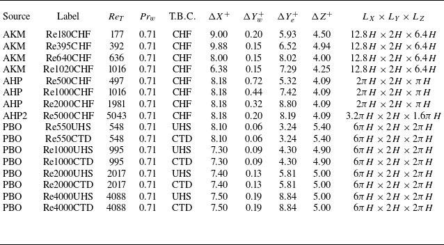
In this paper, incompressible turbulent channel flows (ITCFs) with passive scalar transport are considered as the transformed ‘incompressible’ references. Accordingly, the flow and thermal fields satisfy the incompressible total shear stress (2.6) and the total heat flux (2.15), respectively. The DNS datasets of Abe, Kawamura & Matsuo (Reference Abe, Kawamura and Matsuo2004), Alcántara-Ávila et al. (Reference Alcántara-Ávila, Hoyas and Pérez-Quiles2018, Reference Alcántara-Ávila, Hoyas and Pérez-Quiles2021) and Pirozzoli, Bernardini & Orlandi (Reference Pirozzoli, Bernardini and Orlandi2016) are employed, all featuring a constant molecular Prandtl number
 ${\textit{Pr}} = {\textit{Pr}}_w = 0.71$
, and covering a range of friction Reynolds numbers from
 ${\textit{Re}}_T \approx 180$
to
 ${\textit{Re}}_T \approx 5000$
, as summarised in table 1.
Summary of DNS datasets for ITCFs with passive scalar transport. Data sources are abbreviated as follows: AKM for Abe et al. (Reference Abe, Kawamura and Matsuo2004), AHP for Alcántara-Ávila et al. (Reference Alcántara-Ávila, Hoyas and Pérez-Quiles2018), AHP2 for Alcántara-Ávila et al. (Reference Alcántara-Ávila, Hoyas and Pérez-Quiles2021), and PBO for Pirozzoli et al. (Reference Pirozzoli, Bernardini and Orlandi2016). Here, the friction Reynolds number is defined as
 ${\textit{Re}}_T = Y^+ |_{Y = H}$
, where
 $H$
is the channel half-height. The molecular Prandtl number is denoted by
 ${\textit{Pr}} = {\textit{Pr}}_w = 0.71$
. ‘T.B.C.’ indicates the type of thermal boundary condition applied, including constant wall heat flux (CHF), constant temperature difference (CTD), and uniform heat source (UHS). The grid resolutions in the streamwise and spanwise directions are denoted by
 $\Delta X^+$
and
 $\Delta Z^+$
, respectively, while
 $\Delta Y_w^+$
and
 $\Delta Y_e^+$
represent the wall-normal resolutions at the wall and the channel centreline. The computational domain size is expressed as
 $L_X \times L_Y \times L_Z$
.

The total shear stress in these flows is straightforwardly given by
 $\bar \tau _{t,{\textit{in}}}^+ = 1 - Y/H = 1 - Y^+/{\textit{Re}}_T$
due to the balance between the streamwise pressure gradient and the wall shear stress, where
 $H$
denotes the channel half-height, and
 ${\textit{Re}}_T = Y^+ |_{Y=H}$
. However, it is important to note that the aforementioned studies adopted different strategies for imposing the temperature field, and consequently, the total heat flux
 $\bar q_{t,{\textit{in}}}^+$
depends on the thermal boundary conditions applied. Specifically, for cases with a constant heat flux (CHF) applied at both walls, heat is introduced into the flow, and the total heat flux can be expressed as (Kasagi, Tomita & Kuroda Reference Kasagi, Tomita and Kuroda1992; Abe et al. Reference Abe, Kawamura and Matsuo2004; Alcántara-Ávila et al. Reference Alcántara-Ávila, Hoyas and Pérez-Quiles2018, Reference Alcántara-Ávila, Hoyas and Pérez-Quiles2021)
 \begin{equation} \bar q_{t,{\textit{in}}}^+ = \frac {1}{{\textit{Pr}}_w} \left ( \frac {\partial \bar {\mathcal{T}}}{\partial Y} \right)^+ - \overline {\mathcal{T}^{\prime }V^{\prime }}^+ = 1 - \frac {\int _{0}^{Y^+}{\bar U^+ \mathrm{d} Y^+}}{\int _{0}^{{\textit{Re}}_T}{\bar U^+ \mathrm{d} Y^+}}. \end{equation}
In contrast, for cases with a constant temperature difference (CTD) between the two walls, heat is transferred uniformly from the hotter wall to the cooler one (Lyons, Hanratty & McLaughlin Reference Lyons, Hanratty and McLaughlin1991; Pirozzoli et al. Reference Pirozzoli, Bernardini and Orlandi2016), i.e.
 \begin{equation} \bar q_{t,{\textit{in}}}^+ = \frac {1}{{\textit{Pr}}_w} \left ( \frac {\partial \bar {\mathcal{T}}}{\partial Y} \right)^+ - \overline {\mathcal{T}^{\prime }V^{\prime }}^+ = 1. \end{equation}
Pirozzoli et al. (Reference Pirozzoli, Bernardini and Orlandi2016) imposed a spatially uniform internal heating by adding a source term to the energy equation, ensuring that the bulk temperature remains constant over time. Under this configuration, the total heat flux varies linearly with the wall-normal coordinate and is given by (Pirozzoli et al. Reference Pirozzoli, Bernardini and Orlandi2016; Pirozzoli Reference Pirozzoli2023b )
 \begin{equation} \bar q_{t,{\textit{in}}}^+ = \frac {1}{{\textit{Pr}}_w} \left ( \frac {\partial \bar {\mathcal{T}}}{\partial Y} \right)^+ - \overline {\mathcal{T}^{\prime }V^{\prime }}^+ = 1 - \frac {Y^+}{{\textit{Re}}_T}. \end{equation}
Figures 1(a,b) present the inner-scaled mean streamwise velocity and mean temperature profiles as functions of
 $Y^+$
. Temperature profiles with comparable Reynolds numbers but different thermal boundary conditions exhibit noticeable differences in the outer region, which is consistent with the differences in total heat flux. In the viscous and conductive sublayers, the profiles collapse onto the linear laws
 $\bar {U}^+ = Y^+$
and
 $\bar {\mathcal{T}}^+ = {\textit{Pr}}_w\, Y^+$
, respectively. However, noticeable Reynolds number effects are observed in the logarithmic layer: as the friction Reynolds number
 ${\textit{Re}}_T$
increases, the log-law profiles systematically shift downwards. Only when
 ${\textit{Re}}_T \gtrsim 1000$
do they asymptotically approach the classical laws
 $\bar {U}^+ = \ln Y^+ \!/ 0.41 + 5.2$
and
 $\bar {\mathcal{T}}^+ = \ln Y^+ \!/ 0.48 + 3.9$
(Kays & Crawford Reference Kays and Crawford1993). A similar trend can also be observed in the profiles of eddy thermal conductivity. As shown in figure 1(c), the profiles shift upwards with increasing
 ${\textit{Re}}_T$
in the inner layer, and can be accurately captured by the model proposed by Chen et al. (Reference Chen, Lv, Xu, Shi and Yang2022b
) for
 ${\textit{Re}}_T \gtrsim 1000$
. It is worth noting that such Reynolds number effects have typically been overlooked in previous studies on compressibility transformations (Huang et al. Reference Huang, Coleman, Spalart and Yang2023; Cheng & Fu Reference Cheng and Fu2024a
), where the law of the wall in the high Reynolds number limit was simplistically adopted as the ‘incompressible’ reference to assess transformation accuracy. This approach is theoretically questionable, as compressibility transformations are designed to eliminate Mach number effects, but do not account for Reynolds number dependence (Modesti & Pirozzoli Reference Modesti and Pirozzoli2016; Trettel & Larsson Reference Trettel and Larsson2016; Griffin et al. Reference Griffin, Fu and Moin2023).
The law of the wall for (a) mean streamwise velocity and (b) mean temperature, along with profiles of (c) eddy thermal conductivity and (d) mixed Prandtl number in ITCFs with passive scalar transport. In (a), the grey dashed lines indicate the linear law
 $\bar {U}^+ = Y^+$
in the viscous sublayer and the log law
 $\bar {U}^+ = \ln Y^+ \!/ 0.41 + 5.2$
in the logarithmic layer. In (b), the grey dashed lines represent the linear law
 $\bar {\mathcal{T}}^+ = {\textit{Pr}}_w\, Y^+$
in the conductive sublayer and the log law
 $\bar {\mathcal{T}}^+ = \ln Y^+ \!/ 0.48 + 3.9$
in the logarithmic layer. In (c), the grey solid line shows the eddy thermal conductivity model proposed by Chen et al. (Reference Chen, Lv, Xu, Shi and Yang2022b
),
 $\bar {\lambda }_{t,{\textit{in}}} / \bar {\lambda }_w = {\textit{Pr}}_w\, \kappa _T Y^+ [1 - \exp (-Y^+ \!/ A_T^+) ]^2$
, with
 $\kappa _T = 0.48$
and
 $A_T^+ = 20$
. In (d), the grey and black solid lines represent the
 ${\textit{Pr}}_m$
models proposed by Huang et al. (Reference Huang, Coleman, Spalart and Yang2023) (3.4) and the present study (3.7), respectively.

Figure 1(d) presents the profiles of the mixed Prandtl number
 ${\textit{Pr}}_{m,{\textit{in}}}$
as a function of
 $Y^+$
. For convenience and clarity, three distinct regions are identified. In region I (
 $Y^+ \lesssim 3$
), where molecular diffusion dominates (
 $\bar \mu _w \gg \bar \mu _{t,{\textit{in}}}$
and
 $\bar \lambda _{w} \gg \bar \lambda _{t,{\textit{in}}}$
),
 ${\textit{Pr}}_{m,{\textit{in}}}$
approaches its near-wall limiting value
 ${\textit{Pr}}_w = 0.71$
. In region II (
 $3 \lesssim Y^+ \lesssim 50$
), turbulent diffusion becomes increasingly significant and eventually dominates at
 $Y^+ \approx 50$
, where
 ${\textit{Pr}}_{m,{\textit{in}}}$
reaches a peak value of approximately 1. In region III (
 $Y^+ \gtrsim 50$
), where
 $\bar \mu _{t,{\textit{in}}} \gg \bar \mu _w$
and
 $\bar \lambda _{t,{\textit{in}}} \gg \bar \lambda _w$
,
 ${\textit{Pr}}_{m,{\textit{in}}}$
effectively converges to the turbulent Prandtl number
 ${\textit{Pr}}_{t,{\textit{in}}} = c_{\!p} \bar \mu _{t,{\textit{in}}} / \bar \lambda _{t,{\textit{in}}}$
, which approaches 0.85 at
 $Y^+ \gtrsim 150$
for flows with
 ${\textit{Re}}_T \gtrsim 1000$
. Notably, the profiles in regions I and II nearly collapse, exhibiting a negligible dependence on
 ${\textit{Re}}_T$
, while in region III they exhibit noticeable scatter for cases with
 ${\textit{Re}}_T \lesssim 1000$
. Interestingly, similar observations are also reported in CTCFs when
 ${\textit{Pr}}_{m,{\textit{com}}}$
is plotted under the semi-local wall-normal coordinate
 $y^*$
(Lusher & Coleman Reference Lusher and Coleman2022; Huang et al. Reference Huang, Coleman, Spalart and Yang2023; Zhu et al. Reference Zhu, Zhang, Yang, Ji and Xia2025b
), further suggesting that this behaviour may be largely Mach-independent.
Huang et al. (Reference Huang, Coleman, Spalart and Yang2023) neglected the Reynolds number effect in region III, and characterised the nearly universal
 ${\textit{Pr}}_{m,{\textit{in}}}(Y^+)$
profile by modelling the eddy viscosity and the turbulent Prandtl number, expressed as
 \begin{equation} \begin{aligned} {\textit{Pr}}_{m,{\textit{in}}} &= \frac {1+\bar {\mu }_{t,{\textit{in}}}/\bar {\mu }_w}{1/{\textit{Pr}}_w+\left ( \bar {\mu }_{t,{\textit{in}}}/\bar {\mu }_w \right) /{\textit{Pr}}_{t,{\textit{in}}}},\\ \bar {\mu }_{t,{\textit{in}}}/\bar {\mu }_w &= \kappa Y^+\left [ 1-\exp \left ( -Y^+/A^+ \right) \right ] ^2,\\ {\textit{Pr}}_{t,{\textit{in}}} &= 1.05-0.2\tanh ^3\left ( -Y^+/A_{Pr}^{+} \right) , \\ \end{aligned} \end{equation}
where
 $\kappa = 0.41$
,
 $A^+ = 17$
and
 $A_{Pr}^+ = 70$
. As shown by the grey solid line in figure 1(d), this model effectively captures the behaviour in region III for flows with
 ${\textit{Re}}_T \gtrsim 1000$
. However, it clearly fails to reproduce the universal behaviour observed in region II. To address this limitation, Zhu et al. (Reference Zhu, Zhang, Yang, Ji and Xia2025b
) improved the modelling in regions I and II by introducing a single damping function, given by
 \begin{equation} f_1 ({\textit{Pr}}_w, Y^+) = {\textit{Pr}}_w + (1 - {\textit{Pr}}_w) \left [ 1 - \mathrm{exp}(-Y^+ \!/ A_1^+) \right ]^{n_1}, \end{equation}
where
 $n_1 = 3$
is selected to satisfy the asymptotic behaviour near the wall in ITCFs with isothermal walls, i.e.
 ${\textit{Pr}}_{m,{\textit{in}}} - {\textit{Pr}}_w = \mathcal{O}(Y^{+3})$
. The damping constant
 $A_1^+ = 10$
is determined by fitting DNS data from Lusher & Coleman (Reference Lusher and Coleman2022). It has been demonstrated that (3.5) effectively balances simplicity and the accuracy of the integral mean TV relation for the flow regimes considered in their study (
 ${\textit{Re}}_T \lt 1500$
). To enhance the model accuracy and ensure consistency with the logarithmic-region scaling (Huang, Bradshaw & Coakley Reference Huang, Bradshaw and Coakley1993; Huang & Coleman Reference Huang and Coleman1994; Huang et al. Reference Huang, Coleman, Spalart and Yang2023; Zhu et al. Reference Zhu, Zhang, Yang, Ji and Xia2025b
), we propose a simple model to further incorporate the post-peak behaviour in region III at high Reynolds numbers:
 \begin{equation} f_2 \left(\kappa / \kappa _T, Y^+\right) = 1 + (\kappa / \kappa _T - 1) \frac {\left(Y^+/A_2^+\right)^{n_2}}{1 + \left(Y^+/A_2^+\right)^{n_2}}. \end{equation}
Here,
 $\kappa / \kappa _T = 0.85$
represents the approximately constant turbulent Prandtl number
 ${\textit{Pr}}_{t,{\textit{in}}}$
in the logarithmic region (Kays Reference Kays1994; Lusher & Coleman Reference Lusher and Coleman2022; Huang et al. Reference Huang, Coleman, Spalart and Yang2023). The two empirical parameters
 $A_2^+ = 83$
and
 $n_2 = 4$
are determined by fitting the profiles in the range
 $50 \leqslant Y^+ \leqslant 0.3\, {\textit{Re}}_T$
for the cases listed in table 1 with
 ${\textit{Re}}_T \geqslant 1000$
. Mathematically,
 $A_2^+$
denotes the value of
 $Y^+$
at which
 $f_2 = (1 + 0.85)/2 = 0.925$
, while
 $n_2$
characterises the steepness of the transition. It should be noted that the
 ${\textit{Pr}}_{m,{\textit{in}}}$
behaviour in region III is relatively complex, with the profiles exhibiting Reynolds-number-dependent scatter for
 ${\textit{Re}}_T \lesssim 1000$
, as noted above. Accordingly, the simplified modelling in (3.6) should be regarded as a practical compromise, primarily intended to improve the characterisation for high-Reynolds-number flows.
Given that
 $f_2 \rightarrow 1$
in region I and
 $f_1 \rightarrow 1$
in region III, the full expression for
 ${\textit{Pr}}_{m,{\textit{in}}}$
can be naturally constructed as the product of the two constituent functions:
 \begin{equation} {\textit{Pr}}_{m,{\textit{in}}} = f_1({\textit{Pr}}_w,Y^+) \times f_2(0.85,Y^+). \end{equation}
The performance of (3.7) is represented by the black solid line in figure 1(d). This model, originally formulated to describe the behaviour of
 ${\textit{Pr}}_{m,{\textit{in}}}$
in the high-Reynolds-number limit, is here directly extended to all Reynolds number regimes. Compared to Huang’s model, it demonstrates notable improvements in regions I and II, attributed to the effectiveness of (3.5). Beyond the peak of
 ${\textit{Pr}}_{m,{\textit{in}}}$
, this model also accurately captures the profiles for
 ${\textit{Re}}_T \gtrsim 1000$
, showing close agreement with the
 ${\textit{Pr}}_{t,{\textit{in}}}$
model in (3.4).
4. Assessment of the transformation accuracy
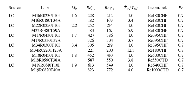
In this section, we systematically evaluate the performance of TL-, GFM-, HLPP-, ZSYX-, SLVD- and VIPL-type velocity and temperature transformations in three canonical CWBTF configurations, including CTCFs with symmetric isothermal walls, CTCFs with asymmetric thermal boundary conditions (i.e. one isothermal cold wall and one adiabatic hot wall), and ZPG CTBLFs with and without wall heat transfer. The assessment is conducted by comparing the transformed profiles with the ‘incompressible’ references (ITCFs with passive scalar transport) at comparable characteristic Reynolds numbers
 ${\textit{Re}}_T$
, as compressibility effects are expected to be eliminated, while the Reynolds-number-dependent effect observed in figure 1 persists. It is worth noting that the wall molecular Prandtl numbers (
 ${\textit{Pr}}_w$
) for all cases fall within the range 0.7–0.72, therefore the differences among them are neglected for simplicity. For quantitative evaluation, the integrated percentage error of a quantity
 $\xi$
is defined as (Cheng & Fu Reference Cheng and Fu2024a
)
 \begin{equation} \varepsilon (\%) = \frac {\int _\alpha ^\beta {\left | \xi _{\textit{trans}} - \xi _{\textit{ref}} \right | \mathrm{d} Y^+}}{\int _\alpha ^\beta {\left | \xi _{\textit{ref}} \right | \mathrm{d} Y^+}} \times 100\,\%, \end{equation}
where
 $\xi _{\textit{trans}}(Y^+)$
denotes the transformed profile (mean velocity
 $\bar U_{\textit{trans}}^+(Y^+)$
or mean temperature
 $\bar {\mathcal{T}}_{\textit{trans}}^+ (Y^+)$
in § 4.1 and § 4.2, or the mean temperature gradient
 $\varPhi _{\textit{trans}} (Y^+) = \partial \bar {\mathcal{T}}_{\textit{trans}}^+ / \partial Y^+$
in § 4.3), and
 $\xi _{\textit{ref}}(Y^+)$
denotes the corresponding ‘incompressible’ reference profiles. The bounds
 $\alpha$
and
 $\beta$
specify the range of integration.
For convenience, the effectiveness of the compressible eddy thermal conductivity models is indirectly assessed by reformulating and interpreting (2.23) and (2.24) within the framework of compressibility transformations. Specifically,
 \begin{equation} 1 + \left ( \frac {\bar \lambda _{t,{\textit{in}}}}{\bar \lambda _w} \right)_{\textit{trans}} = \frac {\bar \tau _{t,{\textit{in}}}^+}{\bar \tau _{t,{\textit{com}}}^+} \frac {{\textit{Pr}}_w}{Pr} \left [ 1 + \left ( \frac {\bar \lambda _{t,{\textit{com}}}}{\bar \lambda } \right)_{\textit{DNS}} \right ] \end{equation}
applies to the original TL- and VIPL-type transformations, while
 \begin{equation} 1 + \left ( \frac {\bar \lambda _{t,{\textit{in}}}}{\bar \lambda _w} \right)_{\textit{trans}} = \frac {\partial \bar U_{{\textit{TL}},m}^+ / \partial \tilde u^+}{\partial \bar U_{\textit{trans}}^+ / \partial \tilde u^+} \frac {{\textit{Pr}}_w}{Pr} \left [ 1 + \left ( \frac {\bar \lambda _{t,{\textit{com}}}}{\bar \lambda } \right)_{\textit{DNS}} \right ] \end{equation}
corresponds to the GFM-, HLPP-, ZSYX- and SLVD-type transformations. Here,
 $( \bar \lambda _{t,{\textit{com}}} / \bar \lambda)_{\textit{DNS}}$
denotes the compressible eddy thermal conductivity obtained from the DNS data, while
 $( \bar \lambda _{t,{\textit{in}}} / \bar \lambda _w)_{\textit{trans}}$
represents the corresponding transformed state associated with the mean velocity scaling
 $\bar U_{\textit{trans}}^+ (Y^+)$
. If the transformation is perfect, then
 $( \bar \lambda _{t,{\textit{in}}} / \bar \lambda _w)_{\textit{trans}}$
is expected to collapse onto the ‘incompressible’ reference when plotted against the transformed coordinate
 $Y^+$
.
In the following analysis, the mixed Prandtl number is assumed to be Mach-number-independent, i.e.
 ${\textit{Pr}}_{m,{\textit{com}}}(Y^+,{\textit{Re}}_T,{\textit{Pr}}_w) = {\textit{Pr}}_{m,{\textit{in}}}(Y^+,{\textit{Re}}_T,{\textit{Pr}}_w)$
(Huang et al. Reference Huang, Coleman, Spalart and Yang2023; Zhu et al. Reference Zhu, Zhang, Yang, Ji and Xia2025b
). The ‘incompressible’ total shear stress is given by
 $\bar \tau _{t,{\textit{in}}}^+ = 1 - Y^+ \!/ {\textit{Re}}_T$
, while the total heat flux
 $\bar q_{t,{\textit{in}}}^+$
is determined by (3.1)–(3.3), depending on the specific thermal boundary condition. Following the convention of previous studies (Griffin et al. Reference Griffin, Fu and Moin2021b
; Bai, Griffin & Fu Reference Bai, Griffin and Fu2022; Zhu et al. Reference Zhu, Song, Yang and Xia2024), each DNS case within a given flow configuration is identified by
 ${\textit{Re}}_T$
(
 ${\textit{Re}}_{\tau ,e}^*$
for
 $Y^+ = y^*$
and
 ${\textit{Re}}_{V,e}$
for
 $Y^+ = y_V^+$
), as it provides a unique characterisation once the compressibility transformation is applied. It should also be noted that Favre-averaged velocity
 $\tilde u$
and temperature
 $\tilde T$
are typically not reported in open-source DNS datasets. Accordingly, they are consistently replaced by the Reynolds-averaged counterparts
 $\bar u$
and
 $\bar T$
when processing these data.
4.1. The CTCFs with symmetric isothermal
 $w$
alls

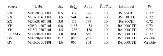
In this subsection, DNS data of CTCFs with symmetric isothermal walls from Zhang & Xia (Reference Zhang and Xia2020), Yao & Hussain (Reference Yao and Hussain2020), Zhang, Song & Xia (Reference Zhang, Song and Xia2023), Li et al. (Reference Li, Chen, Xiao, Mao and Yao2025b
) and Gerolymos & Vallet (Reference Gerolymos and Vallet2024a
) are employed to assess the performance of various transformation methods. The datasets span a range of bulk Mach numbers
 $0.5 \leqslant M_b \leqslant 3.0$
and semi-local Reynolds numbers
 $177 \leqslant {\textit{Re}}_{\tau ,e}^* \leqslant 1483$
, as summarised in table 2.
Summary of DNS datasets for CTCFs with symmetric isothermal walls. Data sources are abbreviated as follows: ZX for Zhang & Xia (Reference Zhang and Xia2020) and Zhang et al. (Reference Zhang, Song and Xia2023), YH for Yao & Hussain (Reference Yao and Hussain2020), LCXMY for Li et al. (Reference Li, Chen, Xiao, Mao and Yao2025b
), and GV for Gerolymos & Vallet (Reference Gerolymos and Vallet2023, Reference Gerolymos and Vallet2024a
,Reference Gerolymos and Vallet
b
). Here, the bulk Mach number is defined as
 $M_b = u_b / \sqrt {\gamma R T_{\textit{ref}}}$
, where
 $u_b$
is the bulk velocity,
 $T_{\textit{ref}}$
is the reference temperature, and
 $\tilde T_w = T_{\textit{ref}}$
is the wall temperature. The characteristic Reynolds numbers are
 ${\textit{Re}}_{\tau ,e}^* = y^* |_{y = \delta _e}$
and
 ${\textit{Re}}_{V,e} = y_V^+ |_{y = \delta _e}$
, where
 $\delta _e = h$
is the channel half-height. ‘Incom. ref.’ refers to the transformed ‘incompressible’ DNS data used for reference, as listed in table 1. Note that the molecular Prandtl number is not constant in cases M07R0990T10I and M16R0970T10I (with consistent
 ${\textit{Pr}}_w \approx 0.71$
at the wall), and the final character ‘I’ in each dataset label denotes the isothermal wall boundary condition.

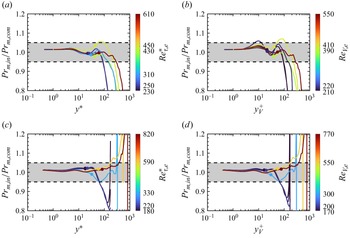
The Mach-independence assumption of the mixed Prandtl number is first examined and validated. As shown in figure 2, the
 ${\textit{Pr}}_{m,{\textit{com}}}$
profiles exhibit a similar collapse to
 ${\textit{Pr}}_{m,{\textit{in}}}$
for
 $Y^+ \lesssim 50$
, regardless of whether
 $Y^+ = y^*$
or
 $Y^+ = y_V^+$
is used. This behaviour is also well captured by the proposed model in (3.7). Beyond the peak region, some deviations are observed for those cases with relatively low Reynolds numbers, as expected. Nevertheless, figure 3 demonstrates that the assumption
 ${\textit{Pr}}_{m,{\textit{com}}}(Y^+,{\textit{Re}}_T,{\textit{Pr}}_w) = {\textit{Pr}}_{m,{\textit{in}}}(Y^+,{\textit{Re}}_T,{\textit{Pr}}_w)$
remains an effective simplification, with the ratio
 ${\textit{Pr}}_{m,{\textit{in}}} / {\textit{Pr}}_{m,{\textit{com}}}$
confined within 0.95–1.05 for
 $Y^+ \leqslant 0.1\, {\textit{Re}}_T$
, thereby covering the entire inner layer (Pope Reference Pope2000).
Compressible mixed Prandtl number
 ${\textit{Pr}}_{m,{\textit{com}}}$
plotted as a function of (a)
 $Y^+ = y^*$
and (b)
 $Y^+ = y_V^+$
in CTCFs with symmetric isothermal walls, based on the DNS datasets listed in table 2. The grey solid and dashed lines indicate the predictions of (3.7) with wall Prandtl numbers
 ${\textit{Pr}}_w = 0.72$
and
 ${\textit{Pr}}_w = 0.71$
, respectively. Hereafter, the colour bar represents the magnitude of the characteristic Reynolds numbers
 ${\textit{Re}}_T$
, providing a unique identifier for each DNS case within a given flow configuration.

Wall-normal distributions of the mixed Prandtl number ratio
 ${\textit{Pr}}_{m,{\textit{in}}} / {\textit{Pr}}_{m,{\textit{com}}}$
in CTCFs with symmetric isothermal walls, plotted as functions of (a)
 $Y^+ = y^*$
and (b)
 $Y^+ = y_V^+$
. Here,
 ${\textit{Pr}}_{m,{\textit{com}}}(Y^+)$
denotes the mixed Prandtl number profiles for the cases listed in table 2, while
 ${\textit{Pr}}_{m,{\textit{in}}}(Y^+)$
corresponds to the ‘incompressible’ reference states with comparable
 ${\textit{Re}}_T$
, as listed in table 1. The theoretical expectation is unity, with the grey shaded region bounded by black dashed lines indicating the
 $\pm$
5 % tolerance band. Filled circles mark the positions
 $Y^+ = 0.1\, {\textit{Re}}_T$
for each case.

To apply the temperature transformation defined in (2.21), it remains to determine
 $\bar \tau _{t,{\textit{com}}}^+$
and
 $B_q \bar q_{t,{\textit{com}}}^+$
. The integral forms of the Reynolds-averaged momentum and total energy equations can be expressed as (Huang, Coleman & Bradshaw Reference Huang, Coleman and Bradshaw1995)
 \begin{equation} \bar {\mu }\frac {\mathrm{d}\tilde {u}}{\mathrm{d}y}+\bar {\mu }\frac {\mathrm{d}\overline {u^{\prime \prime }}}{\mathrm{d}y}+\overline {\mu ^{\prime }\frac {\mathrm{d} u ^{\prime }}{\mathrm{d}y}}-\bar {\rho }\,\widetilde {u^{\prime \prime }v^{\prime \prime }\ } = \bar \tau _w -\int _0^y {\bar F\, \mathrm{d}y}, \end{equation}
 \begin{equation} \overline {\tau _{i2}u_i}-\overline {\rho \tilde {u}_iu_{i}^{\prime \prime }v^{\prime \prime }}-\frac {1}{2}\overline {\rho u_{i}^{\prime \prime }u_{i}^{\prime \prime }v^{\prime \prime }}+\bar {\lambda }\frac {\mathrm{d}\tilde {T}}{\mathrm{d}y}+\bar {\lambda }\frac {\mathrm{d}\overline {T^{\prime \prime }}}{\mathrm{d}y}+\overline {\lambda ^{\prime }\frac {\mathrm{d}T^{\prime }}{\mathrm{d}y}}-c_{\!p}\bar {\rho }\widetilde {T^{\prime \prime }v^{\prime \prime }}=-\bar {q}_w-\!\!\int _0^y{\overline {\textit{Fu}}\mathrm{d}y}, \end{equation}
where
 $\bar F = \bar \tau _w / h$
for flows driven by a uniformly distributed body force. Following the modelling strategies introduced by Zhang et al. (Reference Zhang, Bi, Hussain and She2014) and Huang et al. (Reference Huang, Coleman, Spalart and Yang2023), we adopt the quasi-parallel flow approximation
 $u_i u_i \approx u^2$
and the small turbulence intensity approximation
 $u^2 \approx \tilde u^2 + 2\tilde u u^{\prime \prime }$
. Additionally, the molecular diffusion flux of a quantity
 $\phi$
,
 $\overline {\mu\, \mathrm{d}\phi / \mathrm{d}y}$
, is approximated by its dominant term
 $\bar \mu\, \mathrm{d} \tilde \phi / \mathrm{d}y$
(Huang et al. Reference Huang, Coleman and Bradshaw1995). By combining (4.4) and (4.5), and assuming
 $\overline {\textit{Fu}} \approx \bar F \tilde u$
, the total shear stress and total heat flux can be approximated as (Zhu et al. Reference Zhu, Zhang, Yang, Ji and Xia2025b
)
 \begin{equation} \bar \tau _{t,{\textit{com}}}^+ \approx 1 - y / h \quad \text{and} \quad B_q \bar q_{t,{\textit{com}}}^+ \approx B_q + (\gamma - 1) M_\tau ^2 \int _0^{\tilde u^+}{\bar \tau _{t,{\textit{com}}}^+\, \mathrm{d} \tilde u^+}, \end{equation}
where
 $B_q = \bar q_w / (\bar \rho _w c_{\!p} u_\tau \tilde T_w)$
and
 $M_\tau = u_\tau / \sqrt {\gamma R \tilde T_w}$
. It can be seen that these simplifications intentionally omit higher-order terms that are typically unavailable in open-source DNS datasets, thereby maintaining the simplicity of the formulation, and enhancing its applicability in turbulence modelling (Chen et al. Reference Chen, Huang, Shi, Yang and Lv2022a
; Cheng & Fu Reference Cheng and Fu2024a
). A detailed derivation of (4.6), along with the associated approximations, is provided in Zhu et al. (Reference Zhu, Zhang, Yang, Ji and Xia2025b
). The physical significance of the higher-order terms and the implications of their omission have been thoroughly examined by Huang et al. (Reference Huang, Coleman and Bradshaw1995, Reference Huang, Coleman, Spalart and Yang2023), Lee et al. (Reference Lee, Helm, Martín and Williams2023) and Cheng & Fu (Reference Cheng and Fu2024a
). Furthermore, the performance of the total heat flux approximation is directly evaluated in Appendix C.
Figure 4(a–f) present the transformed mean velocity profiles using the TL, GFM, HLPP, ZSYX, SLVD and VIPL methods, respectively. The corresponding integrated percentage errors, defined by (4.1), are shown in the insets. Here, the integration bounds
 $\alpha = 0$
and
 $\beta = \max \{ 40, 0.1\,{\textit{Re}}_T \}$
are chosen to cover the viscous sublayer, the buffer layer, and at least one-third of the logarithmic region. Theoretically, if a mean velocity scaling is truly Mach-independent, then the transformed profiles should collapse onto their corresponding ‘incompressible’ references at comparable
 ${\textit{Re}}_T$
, thereby minimising the integrated percentage error. Consistent with the results of Zhu et al. (Reference Zhu, Song, Yang and Xia2024), the TL, HLPP and ZSYX transformations demonstrate satisfactory performance, with integrated percentage errors typically below 2 %. Among them, the TL transformation tends to overpredict the mean shear around the buffer layer, which is more pronounced in the case of the GFM transformation. The HLPP transformation shows a downward shift in the log-law intercept due to overcompensation for intrinsic compressibility effects. The ZSYX transformation achieves the highest accuracy, with the transformed profiles nearly collapsing onto the ‘incompressible’ reference, and integrated percentage errors all below 1 %. In contrast, the VIPL and SLVD transformations are found to be unsuitable for symmetric CTCFs, with maximum errors reaching approximately 9 % and 34 %, respectively. This is not surprising, as the former was developed using a data-driven approach based on CTBLF datasets, while the latter was originally proposed as a scaling for the logarithmic region of ZPG CTBLFs.
Transformed mean velocity profiles
 $\bar U_{\textit{trans}}^+ (Y^+)$
in CTCFs with symmetric isothermal walls, based on the DNS datasets listed in table 2. Plots in (a–f) correspond to the TL, GFM, HLPP, ZSYX, SLVD and VIPL transformations, respectively. The grey dashed and solid lines denote the ‘incompressible’ reference profiles at
 ${\textit{Re}}_T \approx 180$
and
 ${\textit{Re}}_T \approx 1000$
, sourced from Lee & Moser (Reference Lee and Moser2015) and Pirozzoli et al. (Reference Pirozzoli, Bernardini and Orlandi2016), respectively. Insets show the errors of all eight cases, with the shaded grey area indicating integrated percentage errors within 2 %. The characteristic Reynolds number
 ${\textit{Re}}_T$
is used to identify the different cases.

Equation (2.19) is first applied with the compressible total heat flux
 $B_q \bar {q}_{t,{\textit{com}}}^+$
extracted directly from the DNS data. For the three cases from Yao & Hussain (Reference Yao and Hussain2020) and Li et al. (Reference Li, Chen, Xiao, Mao and Yao2025b
), however,
 $B_q \bar {q}_{t,{\textit{com}}}^+$
must be modelled using (4.6) due to the lack of the necessary statistical quantities. The corresponding results are presented in figure 5. Ideally, (2.21) preserves the accuracy of the velocity transformation if
 $\bar \tau _{t,{\textit{com}}}^+ = 1 - y/h$
and
 ${\textit{Pr}}_{m,{\textit{com}}}(Y^+,{\textit{Re}}_T,{\textit{Pr}}_w) = {\textit{Pr}}_{m,{\textit{in}}}(Y^+,{\textit{Re}}_T,{\textit{Pr}}_w)$
hold. Specifically, a strictly Mach-independent mean velocity scaling enables an accurate temperature transformation, effectively collapsing the mean temperature profiles onto their corresponding ‘incompressible’ references at similar
 ${\textit{Re}}_T$
. Conversely, if the Mach number independence is not satisfactorily achieved, then the transformed profiles display pronounced scatter and systematic deviations. As observed, the HLPP- and ZSYX-type transformations are the most accurate, with mean integrated percentage errors below 2 %, and minimal scatter. The TL- and GFM-type transformations perform slightly worse due to overprediction in the buffer layer, but they can still be considered effective. In contrast, the SLVD- and VIPL-type transformations continue to be inapplicable. These behaviours are consistent with the corresponding velocity transformations shown in figure 4, suggesting that both the total shear stress approximation and the Mach independence of the mixed Prandtl number are valid, although the overall accuracy is slightly affected.
Transformed mean temperature profiles
 $\bar {\mathcal{T}}_{\textit{trans}}^+ (Y^+)$
in CTCFs with symmetric isothermal walls, where the compressible total heat flux
 $B_q \bar q_{t,{\textit{com}}}^+$
is directly extracted from the DNS data whenever available. Plots in (a–f) correspond to the TL-, GFM-, HLPP-, ZSYX-, SLVD- and VIPL-type transformations, respectively. The grey dashed and solid lines denote the ‘incompressible’ reference profiles at
 ${\textit{Re}}_T \approx 180$
and
 ${\textit{Re}}_T \approx 1000$
, sourced from Abe et al. (Reference Abe, Kawamura and Matsuo2004) and Pirozzoli et al. (Reference Pirozzoli, Bernardini and Orlandi2016), respectively. The characteristic Reynolds number
 ${\textit{Re}}_T$
is used to identify the different cases.

An effective and concise model for
 $B_q \bar {q}_{t,{\textit{com}}}^+$
is highly desirable, as it is essential for eliminating reliance on higher-order statistics and facilitating the application of temperature transformations in near-wall modelling. Figure 6 presents the transformed mean temperature profiles obtained by further employing the approximation (4.6). In this context, the TL-, GFM-, HLPP- and ZSYX-type transformations remain effective, with errors typically remaining below 4 %. The VIPL- and SLVD-type transformations continue to be unsuitable, although the approximation (4.6) partially mitigates their inaccuracies. Notably, this approximation induces visible deviations in the outer region, as
 $B_q \bar {q}_{t,{\textit{com}}}^+$
increases more rapidly from its negative near-wall value toward zero, with these deviations being more significant there, as demonstrated in Appendix C. Specifically, case M30R0180T10I shows a sudden rise in the logarithmic region, while cases M07R0990T10I and M16R0970T10I exhibit singular behaviour. Nevertheless, the performance and accuracy of the transformations in the inner layer are largely unaffected, and the results remain consistent with those in figure 5. Therefore, (4.6) is confirmed to be applicable for this type of flow (Chen et al. Reference Chen, Huang, Shi, Yang and Lv2022a
).
Transformed mean temperature profiles
 $\bar {\mathcal{T}}_{\textit{trans}}^+ (Y^+)$
in CTCFs with symmetric isothermal walls, where the compressible total heat flux
 $B_q \bar q_{t,{\textit{com}}}^+$
is approximated by (4.6) instead. The figure follows the same format and layout as figure 5.

Transformed eddy thermal conductivity profiles
 $( \bar \lambda _{t,{\textit{in}}} / \bar \lambda _w)_{\textit{trans}} (Y^+)$
in CTCFs with symmetric isothermal walls. Plots in (a–f) correspond to the TL-, GFM-, HLPP-, ZSYX-, SLVD- and VIPL-type transformations, respectively. The grey solid lines indicate the damping function model proposed by Chen et al. (Reference Chen, Lv, Xu, Shi and Yang2022b
), while the grey dashed lines represent the ‘incompressible’ reference profiles at
 ${\textit{Re}}_T \approx 180, 395, 550, 1000$
from Abe et al. (Reference Abe, Kawamura and Matsuo2004) and Pirozzoli et al. (Reference Pirozzoli, Bernardini and Orlandi2016). Insets show the near-wall region (
 $Y^+ \in [1, 20]$
), encompassing the viscous sublayer and part of the buffer layer.

Figure 7 presents the transformed eddy thermal conductivity profiles corresponding to the aforementioned transformation methods, by employing (4.2) and (4.3). Note that the three cases from Yao & Hussain (Reference Yao and Hussain2020) and Li et al. (Reference Li, Chen, Xiao, Mao and Yao2025b
) are excluded due to the absence of reported turbulent heat flux data,
 $-c_{\!p} \bar \rho\, \widetilde {T^{\prime \prime }v^{\prime \prime }}$
. As expected from the theoretical analysis in § 2.3, the results closely align with those shown in figure 5. Overall, the TL-, ZSYX- and HLPP-type transformations exhibit excellent performance, with their transformed profiles collapsing onto the corresponding ‘incompressible’ reference across the entire inner layer. As highlighted in the insets, the SLVD-type transformation is the only method that fails in the conductive sublayer (
 $Y^+ \lesssim 5$
), leading to its breakdown in both figures 5 and 6, due to cumulative error propagation. For the high-Mach-number case M30R0180T10I, the GFM- and VIPL-type transformations fall noticeably below the ‘incompressible’ reference in the buffer layer, consistent with their overprediction of
 $\bar {\mathcal{T}}_{\textit{trans}}^+(Y^+)$
observed earlier. Interestingly, despite its failure near the wall, the SLVD-type transformation performs remarkably well in the logarithmic region, whereas the GFM-type transformation exhibits comparatively poorer performance.
4.2. The CTCFs with asymmetric thermal boundary conditions
In this subsection, DNS data of asymmetric CTCFs from Lusher & Coleman (Reference Lusher and Coleman2022) are analysed. The channel configuration consists of an isothermal cold wall and an adiabatic hot wall, and the flows near each wall are considered separately to investigate the effects of wall thermal boundary conditions (Lusher & Coleman Reference Lusher and Coleman2022; Huang et al. Reference Huang, Coleman, Spalart and Yang2023; Cheng & Fu Reference Cheng and Fu2024a
; Zhang, Song & Xia Reference Zhang, Song and Xia2024). The location of the maximum mean streamwise velocity is defined as the effective boundary layer edge, i.e.
 $y = \delta _e,\ \mathrm{d}\tilde u / \mathrm{d}y = 0$
. Here,
 $\delta _e$
represents the effective boundary layer thickness on either the isothermal or adiabatic wall side. The datasets cover a range of bulk Mach numbers
 $1.6 \leqslant M_b \leqslant 3.4$
, with corresponding semi-local Reynolds numbers
 $228 \leqslant {\textit{Re}}_{\tau ,e}^* \leqslant 613$
on the isothermal cold wall side, and
 $182 \leqslant {\textit{Re}}_{\tau ,e}^* \leqslant 823$
on the adiabatic hot wall side, as summarised in table 3.
Summary of DNS datasets for CTCFs with asymmetric thermal boundary conditions. The open-source DNS data from Lusher & Coleman (Reference Lusher and Coleman2022), specifically the cases labelled ‘aiB’, ‘aiC’, ‘aiD’, ‘aiE’, ‘aiD2’ and ‘aiF2’ in their original work, are referred to as LC. The characteristic Reynolds numbers are
 ${\textit{Re}}_{\tau ,e}^* = y^* |_{y = \delta _e}$
and
 ${\textit{Re}}_{V,e} = y_V^+ |_{y = \delta _e}$
, where
 $\delta _e$
denotes the effective boundary layer edge, identified by the condition
 $\mathrm{d}\tilde u / \mathrm{d}y = 0$
(Lusher & Coleman Reference Lusher and Coleman2022; Huang et al. Reference Huang, Coleman, Spalart and Yang2023). Other definitions are consistent with those provided in table 2. The final character in each dataset label indicates the wall thermal boundary condition: ‘I’ for isothermal, and ‘A’ for adiabatic.

The Mach-invariance assumption for the mixed Prandtl number on each wall side is first examined. As shown in figure 8,
 ${\textit{Pr}}_{m,{\textit{com}}}$
demonstrates a satisfactory collapse for
 $Y^+ \lesssim 50$
, which is well captured by (3.7), exhibiting only weak sensitivity to Mach number, Reynolds number, and the wall temperature parameter. On the isothermal cold wall side,
 $Y^+ = y^*$
proves to be a more suitable choice than
 $Y^+ = y_V^+$
, as the latter shows noticeable scatter around
 $Y^+ \approx 10$
. Additionally, the
 ${\textit{Pr}}_{m,{\textit{com}}}(Y^+)$
profiles on the isothermal cold wall side exhibit greater scatter beyond the peak region than those on the adiabatic hot-wall side, which may be attributed to the Reynolds number effects observed in figure 1(d). Nevertheless, the assumption
 ${\textit{Pr}}_{m,{\textit{com}}}(Y^+,{\textit{Re}}_T,{\textit{Pr}}_w) = {\textit{Pr}}_{m,{\textit{in}}}(Y^+,{\textit{Re}}_T,{\textit{Pr}}_w)$
remains valid on both wall sides, as is further confirmed by figure 9, where deviations are confined within
 $\pm$
5 % for
 $Y^+ \leqslant 0.1\, {\textit{Re}}_T$
.
Compressible mixed Prandtl number
 ${\textit{Pr}}_{m,{\textit{com}}}$
plotted as a function of (a,c)
 $Y^+ = y^*$
and (b,d)
 $Y^+ = y_V^+$
, on the (a,b) isothermal and (c,d) adiabatic wall sides of asymmetric CTCFs. The DNS datasets correspond to those summarised in table 3. The grey solid lines represent predictions of (3.7) using wall Prandtl number
 ${\textit{Pr}}_w = 0.7$
.

Wall-normal distributions of the mixed Prandtl number ratio
 ${\textit{Pr}}_{m,{\textit{in}}} / {\textit{Pr}}_{m,{\textit{com}}}$
, plotted as functions of (a,c)
 $Y^+ = y^*$
and (b,d)
 $Y^+ = y_V^+$
on the (a,b) isothermal and (c,d) adiabatic wall sides of asymmetric CTCFs. The DNS datasets correspond to those summarised in table 1 and table 3. Symbols and shading follow the conventions of figure 3.

The mean momentum and total energy equations remain governed by (4.4) and (4.5), except that the mean body force is redefined as
 $\bar F = ( \bar \tau _{w1} + \bar \tau _{w2}) / 2h$
, where
 $\bar \tau _{w1}$
and
 $\bar \tau _{w2}$
denote the absolute values of the mean wall shear stress on the two respective walls, and
 $h$
represents the channel half-height. By adopting the same approximations as in § 4.1, the total shear stress and total heat flux are simplified as (Zhu et al. Reference Zhu, Zhang, Yang, Ji and Xia2025b
)
 \begin{equation} \bar \tau _{t,{\textit{com}}}^+ \approx 1 - y / \delta _e \quad \text{and} \quad B_q \bar q_{t,{\textit{com}}}^+ \approx B_q + (\gamma - 1) M_\tau ^2 \int _0^{\tilde u^+}{\bar \tau _{t,{\textit{com}}}^+\, \mathrm{d} \tilde u^+}, \end{equation}
where
 $y$
and
 $\delta _e$
denote the wall-normal distance and the effective boundary layer thickness adjacent to each wall, respectively.
Figure 10(a–f) present the transformed mean velocity profiles on the isothermal cold wall side, corresponding to the TL, GFM, HLPP, ZSYX, SLVD and VIPL transformations. In this subsection, the integration bounds in (4.1) are also chosen as
 $\alpha = 0$
and
 $\beta = \max \{ 40, 0.1\,{\textit{Re}}_T \}$
. The associated integrated percentage errors are displayed in the insets, with the grey shaded region indicating errors below 2 %. Overall, the performance of these transformations closely resembles that observed in symmetric CTCFs. Among them, the TL and ZSYX transformations are the most accurate, typically yielding errors under 2 %. The GFM and HLPP transformations perform slightly worse, showing overprediction and underprediction around the buffer layer, respectively, though their average errors remain below 4 %. In contrast, the SLVD and VIPL transformations are not applicable on the isothermal cold wall side, and perform worse than in symmetric CTCFs, as the adiabatic wall on the opposite side forces more heat through the isothermal wall. It is worth noting that the TL, HLPP and ZSYX transformations nearly collapse all profiles, aligning closely with the ‘incompressible’ reference at
 ${\textit{Re}}_T \approx 1000$
. While Huang et al. (Reference Huang, Coleman, Spalart and Yang2023) and Cheng & Fu (Reference Cheng and Fu2024a
) regarded such performance to be perfect, the transformed velocity profiles are in fact expected to exhibit a log-law shift due to Reynolds number effects, as discussed in § 3. Our recent study (Zhu et al. Reference Zhu, Song, Zhang, Yang, Ji and Xia2025a
) suggests that this behaviour may be attributed to the modulation effect of the spatially uniform body force
 $F = f_I$
on the flow field, which enhances turbulence intensity on the isothermal cold wall side beyond what is implied by the characteristic Reynolds number
 ${\textit{Re}}_T$
. Incorporating a density-weighted body force
 $F = \rho f_{II}$
(where
 $f_{II}$
is spatially uniform) may yield transformed profiles that more accurately match the corresponding ‘incompressible’ reference.


Figure 11 presents the transformed mean temperature profiles corresponding to the six transformation methods considered. Here,
 $\bar \tau _{t,{\textit{com}}}^+$
is approximated using (4.7), while
 $B_q \bar q_{t,{\textit{com}}}^+$
is directly obtained from the DNS data. Notably, the TL-, HLPP- and ZSYX-type transformations display increased scatter in the logarithmic region, which is mainly attributable to the neglect of fluctuating components in the viscous shear stress approximation. In contrast, the GFM- and VIPL-type transformations benefit from a mutual cancellation of errors, resulting in improved accuracy compared to their velocity counterparts. To further enhance the practicality of the mean temperature transformation, the compressible total heat flux is further approximated using (4.7), and the corresponding results are shown in figure 12. As demonstrated in Appendix C, this approximation is essentially valid under the present flow configuration. Accordingly, the accuracy of the temperature transformations remains largely unaffected. In this context, the GFM-type transformation demonstrates the highest accuracy, with integrated percentage errors typically below 2 %, and minimal scatter. The TL- and ZSYX-type transformations perform slightly less accurately but still yield reliable results, maintaining mean errors below 4 %. The HLPP-type transformation, however, is no longer recommended due to a pronounced downward shift in the logarithmic intercept, with maximum errors reaching up to 7 %.
Transformed mean temperature profiles
 $\bar {\mathcal{T}}_{\textit{trans}}^+ (Y^+)$
on the isothermal wall side of asymmetric CTCFs, where the compressible total heat flux
 $B_q \bar q_{t,{\textit{com}}}^+$
is directly extracted from the DNS data. The figure follows the same format and layout as figure 5.

Transformed mean temperature profiles
 $\bar {\mathcal{T}}_{\textit{trans}}^+ (Y^+)$
on the isothermal wall side of asymmetric CTCFs, where the compressible total heat flux
 $B_q \bar q_{t,{\textit{com}}}^+$
is approximated by (4.7) instead. The figure follows the same format and layout as figure 5.

Figure 13 illustrates the transformed mean velocity profiles on the adiabatic wall side for the six transformation methods under consideration. The performance of these methods aligns well with previously reported behaviours near adiabatic walls (Griffin et al. Reference Griffin, Fu and Moin2021b
; Hasan et al. Reference Hasan, Larsson, Pirozzoli and Pecnik2023; Huang et al. Reference Huang, Coleman, Spalart and Yang2023; Zhu et al. Reference Zhu, Song, Yang and Xia2024). Specifically, the GFM, HLPP, ZSYX and VIPL transformations demonstrate excellent accuracy, with integrated percentage errors typically below 1 %. The TL transformation, while maintaining errors approximately 2 %, exhibits a noticeable upward deviation from the ‘incompressible’ reference profile. It is particularly noteworthy that the SLVD transformation nearly collapses all profiles onto the ‘incompressible’ reference at
 ${\textit{Re}}_T \approx 1000$
, a result previously regarded as favourable by Cheng & Fu (Reference Cheng and Fu2024a
). However, as discussed in § 3, an ideal transformation is in fact expected to reproduce Reynolds-number-dependent shifts in the transformed profiles.


Figure 14 presents the transformed mean temperature profiles, where
 $B_q \bar q_{t,{\textit{com}}}^+$
is directly obtained from the DNS data. Interestingly, the TL-type transformation now proves to be the most accurate, with all errors remaining below 2 % and exhibiting the most concentrated distribution. In contrast, although the GFM, HLPP, ZSYX and VIPL transformations exhibit near-perfect performance for mean velocity, their corresponding temperature transformations perform less favourably at low Reynolds numbers. Comparison with figure 13 suggests that these discrepancies are primarily attributed to the approximation of
 $\bar \tau _{t,{\textit{com}}}^+$
in (4.7) and the assumption
 ${\textit{Pr}}_{m,{\textit{com}}}(Y^+,{\textit{Re}}_T,{\textit{Pr}}_w) = {\textit{Pr}}_{m,{\textit{in}}}(Y^+,{\textit{Re}}_T,{\textit{Pr}}_w)$
. Nevertheless, these methods remain highly effective, with mean errors still below 3 %. The SLVD-type method continues to collapse all profiles onto the high-Reynolds-number ‘incompressible’ reference, which is not expected for an ideal transformation. Figure 15 presents results obtained by further approximating
 $B_q \bar q_{t,{\textit{com}}}^+$
using (4.7). As shown, all transformed profiles lie noticeably above the ‘incompressible’ reference due to overpredictions in the conductive sublayer and buffer layer. This trend aligns with the results of Huang et al. (Reference Huang, Coleman, Spalart and Yang2023), where the authors attributed such discrepancy to low-Reynolds-number effects induced by high temperatures on the adiabatic wall side. However, consistent with the interpretation of Cheng & Fu (Reference Cheng and Fu2024a
), we demonstrate that the deviation primarily arises from the neglect of higher-order terms in the approximation of the compressible total heat flux via (4.7), through comparison with the results shown in figure 14, where
 $B_q \bar q_{t,{\textit{com}}}^+$
is obtained without approximation. Compared to previous results, this effect becomes more pronounced near the adiabatic wall, where the total heat flux approaches zero and the previously neglected terms grow in relative importance, as discussed in Appendix C. Most recently, Zhu et al. (Reference Zhu, Zhang, Yang, Ji and Xia2025b
) validated their proposed integral mean TV relation in asymmetric CTCFs, and found that the model remains highly effective under the same approximation (4.7). In fact, temperature transformations based on strictly Mach-independent mean velocity scalings are essentially equivalent to their integral relation, while avoiding the explicit modelling of
 ${\textit{Pr}}_{m,{\textit{com}}}$
. Therefore, it can be inferred that the inverse form of (2.21), and its further application in near-wall temperature modelling, remain promising.
Transformed mean temperature profiles
 $\bar {\mathcal{T}}_{\textit{trans}}^+ (Y^+)$
on the adiabatic wall side of asymmetric CTCFs, where the compressible total heat flux
 $B_q \bar q_{t,{\textit{com}}}^+$
is directly extracted from the DNS data. The figure follows the same format and layout as figure 5.

Transformed mean temperature profiles
 $\bar {\mathcal{T}}_{\textit{trans}}^+ (Y^+)$
on the adiabatic wall side of asymmetric CTCFs, where the compressible total heat flux
 $B_q \bar q_{t,{\textit{com}}}^+$
is approximated by (4.7) instead. The figure follows the same format and layout as figure 5.

Transformed eddy thermal conductivity profiles
 $( \bar \lambda _{t,{\textit{in}}} / \bar \lambda _w)_{\textit{trans}} (Y^+)$
on the isothermal wall side of asymmetric CTCFs. The figure follows the same format and layout as figure 7.

Transformed eddy thermal conductivity profiles
 $( \bar \lambda _{t,{\textit{in}}} / \bar \lambda _w)_{\textit{trans}} (Y^+)$
on the adiabatic wall side of asymmetric CTCFs. The figure follows the same format and layout as figure 7.

Figures 16 and 17 present the transformed eddy thermal conductivity profiles on the isothermal cold wall and adiabatic hot wall sides, respectively, corresponding to the six transformations. On the isothermal cold wall side, only the SLVD-type transformation fails in the conductive sublayer, while the GFM- and VIPL-type methods exhibit noticeable inaccuracies in the buffer layer. Interestingly, the SLVD-type transformation performs best in the logarithmic region, whereas the other five transformations consistently overestimate the eddy thermal conductivity compared to the ‘incompressible’ reference at a similar characteristic Reynolds number
 ${\textit{Re}}_T$
. This trend is consistent with the earlier observation that the transformed mean velocity and temperature profiles nearly collapse onto ‘incompressible’ profiles with
 ${\textit{Re}}_T \approx 1000$
, and is attributed to turbulence enhancement induced by the spatially uniform body force (Zhu et al. Reference Zhu, Song, Zhang, Yang, Ji and Xia2025a
). On the adiabatic hot wall side, all transformed eddy thermal conductivity profiles show satisfactory agreement with their corresponding ‘incompressible’ references. While the ZSYX- and VIPL-type transformations perform the best, the SLVD-type method slightly overpredicts the eddy thermal conductivity in the buffer layer and logarithmic region, consistent with the profile shifts observed in figures 13 and 14.
4.3. The ZPG CTBLFs with and without wall heat transfer
In this subsection, DNS data for ZPG CTBLFs with adiabatic and diabatic walls from Zhang, Duan & Choudhari (Reference Zhang, Duan and Choudhari2018) and Cogo et al. (Reference Cogo, Baù, Chinappi, Bernardini and Picano2023) are employed to evaluate the performance of various transformation methods. The datasets cover a wide range of freestream Mach numbers
 $2.0 \leqslant M_\infty \leqslant 13.6$
, semi-local Reynolds numbers
 $541 \leqslant {\textit{Re}}_{\tau ,e}^* \leqslant 4952$
, and diabatic parameters
 $0.13 \leqslant \Theta \leqslant 1.00$
, as summarised in table 4. The corresponding DNS profiles of ITCFs with passive scalar transport at similar characteristic Reynolds number
 ${\textit{Re}}_T$
are still considered as the ‘incompressible’ reference.
Summary of DNS datasets for ZPG CTBLFs with and without wall heat transfer. Data sources are abbreviated as follows: ZDC refers to Zhang et al. (Reference Zhang, Duan and Choudhari2018), and CBCBP to Cogo et al. (Reference Cogo, Baù, Chinappi, Bernardini and Picano2023). The freestream Mach number is defined as
 $M_{\infty } = u_{\infty } / \sqrt {\gamma R T_{\infty }}$
, where
 $u_{\infty }$
and
 $T_{\infty }$
denote the freestream velocity and temperature, respectively. The characteristic Reynolds numbers are given by
 ${\textit{Re}}_{\tau ,e}^* = y^* |_{y = \delta _e}$
and
 ${\textit{Re}}_{V,e} = y_V^+ |_{y = \delta _e}$
, where
 $\delta _e = \delta _{99}$
represents the boundary layer thickness at which
 $\bar u \approx 0.99 u_{\infty }$
. The recovery temperature is defined as
 $\tilde T_r = [1 + r (\gamma - 1) M_{\infty }^2 / 2] T_{\infty }$
, and the diabatic parameter
 $\Theta = (\tilde T_w - T_{\infty }) / (\tilde T_r - T_{\infty })$
is used to characterise wall heat transfer effects (Zhang et al. Reference Zhang, Bi, Hussain and She2014; Cogo et al. Reference Cogo, Baù, Chinappi, Bernardini and Picano2023, Reference Cogo, Chinappi, Bernardini and Picano2024; Gibis et al. Reference Gibis, Sciacovelli, Kloker and Wenzel2024).

Wall-normal distributions of the mixed Prandtl number ratio
 ${\textit{Pr}}_{m,{\textit{in}}} / {\textit{Pr}}_{m,{\textit{com}}}$
in ZPG CTBLFs, plotted as functions of (a)
 $Y^+ = y^*$
and (b)
 $Y^+ = y_V^+$
, based on the DNS datasets listed in table 4. Symbols and shading follow the conventions of figure 3.

Figure 18 presents the distributions of the mixed Prandtl number ratio
 ${\textit{Pr}}_{m,{\textit{in}}} / {\textit{Pr}}_{m,{\textit{com}}}$
in ZPG CTBLFs, based on the open-source DNS dataset of Zhang et al. (Reference Zhang, Duan and Choudhari2018). It should be noted that the computed
 ${\textit{Pr}}_{m,{\textit{com}}}$
is subject to approximation errors, as the simplifications
 $-\bar \rho\, \widetilde {u^{\prime \prime }v^{\prime \prime }\ } \approx -\bar \rho\, \overline {u^{\prime }v^{\prime }}$
and
 ${\textit{Pr}}_t \approx (\overline {\rho u^{\prime }v^{\prime }}\, \partial \bar T \!/ \partial y) / (\overline {\rho v^{\prime }T^{\prime }}\, \partial \bar u / \partial y)$
were employed due to unavailable turbulence statistics. For most of the region with
 $Y^+ \leqslant 0.1\, {\textit{Re}}_T$
, the ratio remains nearly within 0.95–1.05. However, using
 $Y^+=y^*$
produces noticeably larger deviations than
 $Y^+=y_V^+$
, with relative errors in parts of the buffer layer exceeding the
 $\pm$
5 % tolerance band. This indicates that the transformed coordinate
 $Y^+=y_V^+$
associated with the VIPL transformation may more effectively eliminate Mach number effects in this flow configuration. Notably, a pronounced singularity occurs near the mean temperature peak (where
 $\partial \tilde T \!/ \partial y = 0$
) for cases with cold walls, suggesting a local breakdown of the assumption
 ${\textit{Pr}}_{m,{\textit{com}}}(Y^+,{\textit{Re}}_T,{\textit{Pr}}_w) = {\textit{Pr}}_{m,{\textit{in}}}(Y^+,{\textit{Re}}_T,{\textit{Pr}}_w)$
. The origin of this singularity and the validity of the current model (3.7) will be discussed and examined in detail below.
Figure 19(a–f) present the transformed mean velocity profiles using the TL, GFM, HLPP, ZSYX, SLVD and VIPL methods, respectively. The integration bounds in (4.1) are set as
 $\alpha = 0$
and
 $\beta = \max \{ 80, 0.1\,{\textit{Re}}_T \}$
, ensuring coverage of the viscous sublayer, the buffer layer, and at least one-third of the logarithmic region. The results are generally consistent with previous studies (Volpiani et al. Reference Volpiani, Iyer, Pirozzoli and Larsson2020; Griffin et al. Reference Griffin, Fu and Moin2021b
; Hasan et al. Reference Hasan, Larsson, Pirozzoli and Pecnik2023; Zhu et al. Reference Zhu, Song, Yang and Xia2024). Specifically, the TL and SLVD transformations exhibit significant scatter around the buffer layer and are therefore not considered applicable. The HLPP transformation clearly improves upon the TL method by accounting for the upward shift of the log-law induced by intrinsic compressibility effects, characterised by the wall friction Mach number
 $M_\tau$
. Nevertheless, the transformed profiles still show noticeable scatter, and the extent of the logarithmic region is generally reduced compared to the ‘incompressible’ references. Accordingly, the integrated percentage errors tend to increase with
 ${\textit{Re}}_{\tau ,e}^*$
. In contrast, the GFM, ZSYX and VIPL transformations demonstrate satisfactory agreement with the corresponding ‘incompressible’ profiles across the entire inner layer, with all errors remaining below 6 %, and mean errors nearly below 2 %.
Transformed mean velocity profiles
 $\bar U_{\textit{trans}}^+ (Y^+)$
in ZPG CTBLFs with and without wall heat transfer, based on the DNS datasets listed in table 4. Plots in (a–f) correspond to the TL, GFM, HLPP, ZSYX, SLVD and VIPL transformations, respectively. The grey dashed and solid lines denote the ‘incompressible’ reference profiles at
 ${\textit{Re}}_T \approx 1000$
and
 ${\textit{Re}}_T \approx 5000$
, sourced from Pirozzoli et al. (Reference Pirozzoli, Bernardini and Orlandi2016) and Alcántara-Ávila et al. (Reference Alcántara-Ávila, Hoyas and Pérez-Quiles2021), respectively. Insets show the errors of all 11 cases, where closed ‘
 $\square$
’ symbols denote the five cases from Zhang et al. (Reference Zhang, Duan and Choudhari2018), and open ‘
 $\square$
’ symbols denote the six cases from Cogo et al. (Reference Cogo, Baù, Chinappi, Bernardini and Picano2023). The shaded grey area indicates integrated percentage errors below 2 %. The characteristic Reynolds number
 ${\textit{Re}}_T$
is used to identify the different cases.

To apply the temperature transformations defined in (2.21), we derive a simplified expression for the compressible total heat flux by adopting approximations similar to those in § 4.1 and § 4.2 (see Appendix B for details):
 \begin{equation} B_q \bar q_{t,{\textit{com}}}^+ \approx B_q + (\gamma -1) M_\tau ^2 \int _{0}^{\tilde u^+}{\bar \tau _{t,{\textit{com}}}^+\, \mathrm{d}\tilde u^+} + \int _1^{\bar \tau _{t,{\textit{com}}}^+}{\frac {\partial \theta }{\partial \tilde u^+}\, \mathrm{d}\bar \tau _{t,{\textit{com}}}^+}. \end{equation}
Compared to (4.6), the third term on the right-hand side accounts for the convective transport of mean enthalpy. While this term can be neglected for further simplification by assuming
 $\bar \tau _{t,{\textit{com}}}^+ \approx 1$
across the entire boundary layer, we retain it in this subsection due to its notable influence in the outer part of the logarithmic region. In the absence of an analytical expression for the total shear stress, we adopt a defect power-law model (Sun & Childs Reference Sun and Childs1973) to approximate its distribution, i.e.
 $\bar \tau _{t,{\textit{com}}}^+ \approx 1 - (y / \delta _e)^{3/2}$
, following the approach of previous studies (Chen & She Reference Chen and She2016; Wu et al. Reference Wu, Bi, Hussain and She2017; Zhu et al. Reference Zhu, Song, Yang and Xia2024).
Before proceeding further, it is important to highlight some challenges in dealing with ZPG CTBLFs over cold walls (i.e.
 $\Theta \lt 1$
or
 $\tilde T_w / \tilde T_r \lt 1$
). In these flows, the mean temperature profiles exhibit non-monotonic variations in the wall-normal direction, primarily due to the combined effects of wall heat transfer and viscous heating. Near the mean temperature peak, the turbulent heat flux also approaches zero. However, a non-negligible discrepancy exists between the wall-normal locations where
 $\bar \lambda\, \partial \tilde T \!/ \partial y$
and
 $-c_{\!p} \bar \rho\, \widetilde {T^{\prime \prime }v^{\prime \prime }}$
vanish. This mismatch becomes increasingly pronounced with rising friction Mach number
 $M_\tau$
, reaching up to a 25 % offset when
 $M_\tau \approx 0.23$
, as reported by Gibis et al. (Reference Gibis, Sciacovelli, Kloker and Wenzel2024). Yet it remains unclear whether this behaviour arises from an underlying physical mechanism or from numerical artefacts. A particularly challenging issue is that the eddy thermal conductivity,
 $\bar \lambda _t = -c_{\!p} \bar \rho\, \widetilde {T^{\prime \prime }v^{\prime \prime }} / (\partial \tilde T \!/ \partial y)$
, becomes ill-defined near the temperature peak, further leading to singularities in both the turbulent and mixed Prandtl numbers, as observed in figure 18 (Chen et al. Reference Chen, Gan and Fu2024; Gibis et al. Reference Gibis, Sciacovelli, Kloker and Wenzel2024). Furthermore, according to (2.21), the transformed mean temperature profiles exhibit abrupt jumps near the zero-crossing point of the total heat flux (Cheng & Fu Reference Cheng and Fu2024a
; Chen et al. Reference Chen, Gan and Fu2025), which lies between the zero points of the molecular and turbulent heat fluxes. Consequently, the methods for directly evaluating
 $\bar {\mathcal{T}}_{\textit{trans}}^+(Y^+)$
presented in § 4.1 and § 4.2 cannot be reliably applied to ZPG CTBLFs.
To mitigate the impact of the discontinuities, we define the mean temperature gradient of the ‘incompressible’ state
 $\varPhi (Y^+) = \partial \bar {\mathcal{T}}^+ \!/ \partial Y^+$
as
 $\xi$
in (4.1), as suggested by Cheng & Fu (Reference Cheng and Fu2024a
). This enables separate quantitative assessments for various transformation methods in the conductive sublayer (
 $\alpha = 0$
,
 $\beta = 5$
) and logarithmic region (
 $\alpha = 30$
,
 $\beta = \max \{ 80, 0.1\,{\textit{Re}}_T \}$
). The results are illustrated in figures 20 and 21, where
 $\varPsi _{\textit{trans}} = Y^+ \varPhi _{\textit{trans}} = Y^+\, \partial \bar {\mathcal{T}}_{\textit{trans}}^+ / \partial Y^+$
is the transformed indicator function. Meanwhile, figure 22 shows the corresponding integrated percentage errors as functions of
 ${\textit{Re}}_T$
. It should be noted that the adiabatic case (
 $\Theta = 1$
), along with the five moderately cooled cases (
 $0 \leqslant \Theta \lt 0.43$
), is used to assess accuracy in the conductive sublayer, as any discontinuity (if present) lies within the buffer layer. Conversely, the adiabatic case, together with the five weakly cooled cases (
 $0.43 \leqslant \Theta \lt 1$
), is used to evaluate performance in the logarithmic region, where any singularity (if present) is confined to the conductive sublayer (Gibis et al. Reference Gibis, Sciacovelli, Kloker and Wenzel2024). To evaluate the intrinsic accuracy of various transformation methods, the compressible total heat flux
 $B_q \bar {q}_{t,{\textit{com}}}^+$
is directly computed from the available turbulence statistics in the five cases reported by Zhang et al. (Reference Zhang, Duan and Choudhari2018). In contrast, for the six cases presented by Cogo et al. (Reference Cogo, Baù, Chinappi, Bernardini and Picano2023),
 $B_q \bar {q}_{t,{\textit{com}}}^+$
is modelled by (4.8), due to the unavailability of the required statistical data. Overall, the performance of these transformation methods is highly consistent with that shown in figure 19. Specifically, most transformations yield mean errors typically below 5 % in the conductive sublayer, indicating generally good performance. However, the SLVD-type transformation fails in the two coldest-wall cases (
 $\Theta \lt 0.2$
), with maximum integrated errors reaching approximately 23 %. Although relative errors are not explicitly quantified, the TL-type transformation exhibits significant overprediction near the end of the buffer layer (
 $20 \lesssim Y^+ \lesssim 30$
). The HLPP- and ZSYX-type transformations offer partial improvements by incorporating intrinsic compressibility effects within their respective mean velocity scalings, but still exhibit noticeable scatter, particularly for cases with
 ${\textit{Re}}_{\tau ,e}^* \gt 4000$
. In contrast, the GFM-, SLVD- and VIPL-type transformations show minimal scatter. In the logarithmic region, the GFM-, ZSYX- and VIPL-type transformations demonstrate superior accuracy, with transformed profiles collapsing closely onto the ‘incompressible’ references at comparable
 ${\textit{Re}}_T$
, and the corresponding mean errors remaining below 5 %. It is worth noting that the SLVD transformation, previously regarded as effective within the logarithmic region, fails to exhibit satisfactory performance in the present study. This discrepancy is primarily attributed to the broader evaluation range adopted here (
 $\alpha = 30$
,
 $\beta = \max \{80,0.1\,{\textit{Re}}_T\}$
), in contrast to that (
 $\alpha = 30$
,
 $\beta = 80$
) used by Cheng & Fu (Reference Cheng and Fu2024a
). The present criterion ensures that at least one-third of the logarithmic region is included for flows with
 ${\textit{Re}}_T \gt 800$
, thereby providing a more rigorous and representative assessment.
Transformed indicator function
 $\varPsi _{\textit{trans}}(Y^+) = Y^+\, \partial \bar {\mathcal{T}}_{\textit{trans}}^+ / \partial Y^+$
in the conductive sublayer of ZPG CTBLFs with and without wall heat transfer. The grey dashed and solid lines represent the ‘incompressible’ reference profiles at
 ${\textit{Re}}_T \approx 1000$
and
 ${\textit{Re}}_T \approx 5000$
, obtained from Pirozzoli et al. (Reference Pirozzoli, Bernardini and Orlandi2016) and Alcántara-Ávila et al. (Reference Alcántara-Ávila, Hoyas and Pérez-Quiles2021), respectively.

Transformed indicator function
 $\varPsi _{\textit{trans}}(Y^+) = Y^+\, \partial \bar {\mathcal{T}}_{\textit{trans}}^+ / \partial Y^+$
in the logarithmic region of ZPG CTBLFs with and without wall heat transfer. The grey dashed and solid lines represent the ‘incompressible’ reference profiles at
 ${\textit{Re}}_T \approx 1000$
and
 ${\textit{Re}}_T \approx 4000$
, obtained from Pirozzoli et al. (Reference Pirozzoli, Bernardini and Orlandi2016).

Integrated percentage errors of the ‘incompressible’ mean temperature gradient,
 $\varPhi (Y^+) = \partial \bar {\mathcal{T}}^+ \!/ \partial Y^+$
, as functions of the characteristic Reynolds number
 ${\textit{Re}}_T$
in ZPG CTBLFs, evaluated within (a) the conductive sublayer and (b) the logarithmic region. Colour and symbol conventions follow those in figure 19.

Transformed eddy thermal conductivity profiles
 $(\bar {\lambda }_{t,{\textit{in}}} / \bar {\lambda }_w)_{\textit{trans}}(Y^+)$
in ZPG CTBLFs with and without wall heat transfer. Plots in (a–f) correspond to the TL-, GFM-, HLPP-, ZSYX-, SLVD- and VIPL-type transformations, respectively. The grey solid lines indicate the damping function model proposed by Chen et al. (Reference Chen, Lv, Xu, Shi and Yang2022b
), while the grey dashed lines represent the ‘incompressible’ reference profiles at
 ${\textit{Re}}_T \approx 1000$
and
 ${\textit{Re}}_T \approx 5000$
, obtained from Pirozzoli et al. (Reference Pirozzoli, Bernardini and Orlandi2016) and Alcántara-Ávila et al. (Reference Alcántara-Ávila, Hoyas and Pérez-Quiles2021).

Figure 23 presents the transformed eddy thermal conductivity profiles associated with the aforementioned transformation methods, computed using (4.2) and (4.3). Only the five cases from Zhang et al. (Reference Zhang, Duan and Choudhari2018) are included, due to the availability of the necessary turbulence statistics. As previously noted, the cases with cold walls exhibit pronounced discontinuities below the buffer layer (
 $Y^+ \lesssim 30$
), attributed to the misalignment in the wall-normal positions of the zero crossings between
 $\bar \lambda\, \partial \tilde {T} \!/ \partial y$
and
 $-c_{\!p} \bar {\rho }\, \widetilde {T^{\prime \prime }v^{\prime \prime }}$
. Within the viscous sublayer (
 $Y^+ \lesssim 5$
), most transformation methods perform well, whereas the SLVD-type transformation shows notable scatter in the two coldest-wall cases, even when the discontinuity effects are excluded. In the logarithmic region, profiles associated with the TL- and HLPP-type transformations fall significantly below the corresponding ‘incompressible’ references for
 $y^* \gtrsim 200$
, leading to deviations from the classical logarithmic law in the outer layer of
 $\bar {\mathcal{T}}_{\textit{trans}}^+(Y^+)$
. Conversely, the SLVD-type transformation yields considerably higher values than the ‘incompressible’ references. The GFM-, ZSYX- and VIPL-type transformations, however, demonstrate excellent performance, with the transformed profiles closely collapsing onto the ‘incompressible’ reference profiles at comparable
 ${\textit{Re}}_T$
. As anticipated from the theoretical analysis in § 2.3, these results are in close agreement with those observed in figure 19, confirming that advanced mean velocity scalings offer strong potential for the development of more accurate compressible eddy thermal conductivity models.
5. Potential and challenges in near-wall temperature modelling
In this section, we investigate the potential of applying integral mean TV relations and temperature transformations, which are directly derived from the mean energy equation, for developing temperature wall models. As a representative class of flow scenarios, ZPG CTBLFs with and without wall heat transfer are primarily considered. Notably, the cold-wall cases present significant modelling challenges due to singularities or discontinuities in the turbulent eddy thermal conductivity, mixed Prandtl number, and transformed mean temperature profiles, as discussed in § 4.3. Accordingly, we also seek to explore potential strategies for handling non-monotonic mean temperature distributions. As this is not the main focus of the present study, we primarily conduct a priori assessments based on the DNS dataset of Zhang et al. (Reference Zhang, Duan and Choudhari2018), which provides comprehensive turbulence statistics.
Recently, Zhu et al. (Reference Zhu, Zhang, Yang, Ji and Xia2025b ) derived an integral mean TV relation for CTCFs directly from the mean momentum and total energy equations. Following a similar approach, a corresponding relation for ZPG CTBLFs can be obtained by reformulating the compressible total heat flux equation as
 \begin{equation} \theta = 1 - \tilde T \!/ \tilde T_w = \int _{0}^{\tilde u^+}{\frac {{\textit{Pr}}_{m,{\textit{com}}}}{\bar \tau _{t,{\textit{com}}}^+} B_q \bar q_{t,{\textit{com}}}^+\, \mathrm{d} \tilde u^+}. \end{equation}
Here, the mixed Prandtl number
 ${\textit{Pr}}_{m,{\textit{com}}}$
is assumed to be independent of Mach numbers with respect to the semi-local coordinate
 $Y^+ = y^*$
, and is thus expected to be modelled by (3.7), given its demonstrated effectiveness in CTCFs. However, such simplification should be carefully assessed, particularly in ZPG CTBLFs with cold walls, where
 ${\textit{Pr}}_{m,{\textit{com}}}$
is ill-defined around the temperature peak. The compressible total shear stress and total heat flux can be modelled by
 $\bar \tau _{t,{\textit{com}}}^+ \approx 1 - (y / \delta _e)^{3/2}$
and (4.8), respectively, to approximately account for the convective effects. Nevertheless, since near-wall temperature models are typically applied below the logarithmic region in high-Reynolds-number flows, the constant-stress approximation
 $\bar \tau _{t,{\textit{com}}}^+ \approx 1$
is often adopted for simplicity. Accordingly, (5.1) reduces to
 \begin{equation} \theta = 1 - \tilde T \!/ \tilde T_w = \int _{0}^{\tilde u^+}{{\textit{Pr}}_{m,{\textit{com}}} \left [ B_q + (\gamma - 1) M_\tau ^2 \tilde u^+ \right ] \mathrm{d} \tilde u^+}. \end{equation}
In addition, the influence of the total heat flux approximation on the overall model accuracy requires further investigation.
Comparison of mean temperature profiles
 $\tilde {T} \!/ \tilde {T}_w$
as functions of
 $y^*$
, obtained from DNS data (grey open ‘
 $\square$
’ symbols), the GRA relation (1.3) (red solid lines), the integral mean TV relation (5.1), and its various approximated forms. The blue dashed lines represent results from the proposed integral TV relation under the constant-stress layer assumption,
 $\bar \tau _{t,{\textit{com}}}^+ \approx 1$
. The green dash-dotted lines include additional modelling of the compressible mixed Prandtl number
 ${\textit{Pr}}_{m,{\textit{com}}}$
using (3.7) with
 $Y^+ = y^*$
, while the magenta dotted lines further incorporate the approximation of the compressible total heat flux
 $B_q \bar q_{t,{\textit{com}}}^+$
, as described in (5.2).

Figure 24 provides a detailed comparison between the mean temperature profiles constructed from various mean TV relations and the DNS data (grey symbols). The red solid lines denote the results from the GRA relation (1.3), which demonstrate nearly perfect agreement across cases with varying levels of wall cooling, consistent with previous findings (Duan & Martin Reference Duan and Martin2011; Zhang et al. Reference Zhang, Duan and Choudhari2018; Cogo et al. Reference Cogo, Baù, Chinappi, Bernardini and Picano2023). However, the GRA relation explicitly relies on boundary-layer-edge quantities, thereby limiting the corresponding temperature wall model from being truly self-determined (Cheng & Fu Reference Cheng and Fu2024a
; Chen et al. Reference Chen, Gan and Fu2025). The blue dashed lines represent the results of the integral relation (5.1), where
 ${\textit{Pr}}_{m,{\textit{com}}}$
and
 $B_q \bar q_{t,{\textit{com}}}^+$
are directly calculated from DNS turbulence statistics, while the constant-stress approximation,
 $\bar \tau _{t,{\textit{com}}}^+ \approx 1$
, is applied. As expected, while the omission of convective effects leads to noticeable discrepancies in the outer region, the obtained mean temperature profiles closely match the DNS data in the logarithmic region and below, which is sufficient for near-wall modelling applications. Subsequently,
 ${\textit{Pr}}_{m,{\textit{com}}}$
is modelled using (3.7) with
 $Y^+ = y^*$
, and the corresponding results are shown as green dash-dotted lines. Interestingly, the resulting profiles deviate only slightly near the temperature peak and in the outer region compared to the results based on DNS-based
 ${\textit{Pr}}_{m,{\textit{com}}}$
(blue dashed lines). This confirms the effectiveness of (3.7) in ZPG CTBLFs, and justifies the simplification of neglecting the singularities near the temperature peak observed in figure 18, as their impact on overall accuracy is limited. Building upon this, the magenta dotted lines show results obtained by additionally applying the total heat flux approximation, leading to the simplified relation given in (5.2). Compared to the green dash-dotted lines, this model performs effectively and even more accurately in the two weakly cooled cases (figure 24
a,b), likely due to partial error cancellation. However, noticeable deviations emerge at
 $y^* \gtrsim 40$
for the two moderate-cooling cases (figure 24
c,d), indicating that the model does not retain consistent and sufficient accuracy throughout the entire region below the logarithmic layer. Further discussion on the impact of the total heat flux approximation is provided in Appendix C.
Another approach is to extend the incompressible law of the wall to high-speed flows via compressibility transformations. Numerous previous studies have successfully applied velocity transformations to construct wall models, significantly enhancing the accuracy of inner layer velocity predictions (Yang & Lv Reference Yang and Lv2018; Hendrickson et al. Reference Hendrickson, Subbareddy and Candler2022, Reference Hendrickson, Subbareddy, Candler and Macdonald2023; Griffin et al. Reference Griffin, Fu and Moin2023; Chen et al. Reference Chen, Gan and Fu2024). In contrast, the application of mean temperature transformations has received comparatively limited attention. Recently, Modesti & Pirozzoli (Reference Modesti and Pirozzoli2024) proposed a closed-form wall model for variable-property forced air convection, solved iteratively by coupling mean temperature and velocity transformations. However, the situation becomes considerably more complex in ZPG CTBLFs with cold walls, where the compressible total heat flux lacks an analytical expression, and the transformation becomes ill-defined near the temperature peak, posing significant challenges and limitations for practical applications (Cheng & Fu Reference Cheng and Fu2024a
; Chen et al. Reference Chen, Gan and Fu2025). Given that the discontinuity is actually caused by the zero-crossing of
 $B_q \bar q_{t,{\textit{com}}}^+$
, which does not coincide with the location where
 $\bar \lambda\, \partial \tilde {T} \!/ \partial y = 0$
, we rewrite (2.21) and reinterpret it as an inverse temperature transformation:
 \begin{equation} \theta = 1 - \tilde T \!/ \tilde T_w = \int _{0}^{\bar {\mathcal{T}}^+}{\frac {{\textit{Pr}}_{m,{\textit{com}}}}{{\textit{Pr}}_{m,{\textit{in}}}} \frac {\bar \tau _{t,{\textit{in}}}^+}{\bar \tau _{t,{\textit{com}}}^+} \frac {B_q \bar q_{t,{\textit{com}}}^+}{\bar q_{t,{\textit{in}}}^+} \left ( \frac {\partial \bar U^+}{\partial \tilde u^+} \right)^{-1} \mathrm{d} \bar {\mathcal{T}}^+}. \end{equation}
Here,
 $(\partial \bar U^+ \!/ \partial \tilde u^+)^{-1}$
acts as the inverse transformation kernel for velocity, which can be determined based on the detailed information provided in Appendix A. The ‘incompressible’ reference profile
 $\bar {\mathcal{T}}^+(Y^+)$
at comparable
 ${\textit{Pr}}_w$
and
 ${\textit{Re}}_T$
can be obtained from explicit composite formulations (Nagib & Chauhan Reference Nagib and Chauhan2008; Pirozzoli Reference Pirozzoli2023a
; Pirozzoli & Modesti Reference Pirozzoli and Modesti2024), direct solutions of (3.1)–(3.3) using the
 ${\textit{Pr}}_{m,{\textit{in}}}$
model (3.7), or available DNS datasets.
Comparison of mean temperature profiles
 $\tilde {T} \!/ \tilde {T}_w$
as functions of
 $y^+$
, obtained from DNS data (grey open ‘
 $\square$
’ symbols), and from the inverse TL (black), GFM (green), HLPP (red), ZSYX (blue), SLVD (cyan) and VIPL type (magenta) temperature transformations. The compressible total heat flux,
 $B_q \bar {q}_{t,{\textit{com}}}^+$
, is approximated using relevant turbulence statistics extracted from DNS data. Note that only the portion of the compressible profiles corresponding to
 $Y^+ \leqslant 0.3\, {\textit{Re}}_T$
is shown, ensuring complete coverage of the wall layers below the logarithmic region in the transformed ‘incompressible’ reference profiles.

Figure 25 compares compressible mean temperature profiles reconstructed via various inverse transformations against DNS data (grey symbols). Here, the Mach-invariance assumption for the mixed Prandtl number,
 ${\textit{Pr}}_{m,{\textit{com}}}(Y^+,{\textit{Re}}_T,{\textit{Pr}}_w) = {\textit{Pr}}_{m,{\textit{in}}}(Y^+,{\textit{Re}}_T,{\textit{Pr}}_w)$
, is consistently employed. The compressible total shear stress is modelled as
 $\bar \tau _{t,{\textit{com}}}^+ \approx 1 - (y / \delta _e)^{3/2}$
, while the compressible total heat flux
 $B_q \bar q_{t,{\textit{com}}}^+$
and the inverse velocity transformation kernel
 $(\partial \bar U^+ \!/ \partial \tilde u^+)^{-1}$
are directly computed from the relevant turbulence statistics to preserve the intrinsic accuracy of the transformation. For convenience, the ‘incompressible’ reference temperature profiles
 $\bar {\mathcal{T}}^+(Y^+)$
are directly extracted from DNS data of ITCFs with passive scalar transport at comparable
 ${\textit{Re}}_T$
, as detailed in tables 1 and 4. Since compressibility transformations are generally valid only within the inner layer, the analysis is restricted to
 $Y^+ \leqslant 0.3\, {\textit{Re}}_T$
, which fully encompasses the conductive sublayer, buffer layer and logarithmic region of the transformed ‘incompressible’ state, and is sufficient for near-wall modelling purposes. As expected, the performance of various transformation methods closely aligns with that shown in figures 20 and 21, given that the present procedure essentially constitutes an inverse mapping. Specifically, the TL- and HLPP-type transformations are not recommended due to their poor accuracy near the buffer layer, while the SLVD-type transformation primarily fails in the conductive sublayer for cases with very cold walls (
 $\Theta \lt 0.2$
). In contrast, the GFM-, ZSYX- and VIPL-type transformations demonstrate superior accuracy and robustness, with weaker sensitivity to Mach number and wall temperature variations. Overall, these findings consistently demonstrate the effectiveness of using the ideal ‘incompressible’ reference profiles as the transformed ‘incompressible’ states within the inverse transformation framework, thereby avoiding the challenges arising from discontinuities in the forward-transformed profiles.
It should be emphasised that the present analysis is limited to the direct validation of (5.2) and (5.3) using DNS data, specifically in addressing non-monotonic mean temperature behaviour in ZPG CTBLFs with cold walls. To develop a predictive wall model, it is further necessary to incorporate the incompressible laws of the wall (1.1) and (1.2), a velocity transformation from Appendix A, the viscosity law
 $\bar \mu \sim \tilde T$
, and the perfect-gas and boundary layer assumptions
 $\bar p = \bar \rho R \tilde T = \textit{const.}$
Theoretically, when combined with a velocity transformation, the wall models constructed from (5.1) or (5.3) are equivalent, as they essentially solve the simplified mean momentum and energy equations, with compressible eddy viscosity and eddy thermal conductivity modelled as described in § 2.2 and § 2.3. When the total shear stress and total heat flux are closed via (4.6)–(4.8), the wall model predicts both the wall shear stress and heat flux, along with mean flow profiles within the modelled region (
 $y \in [0,y_m]$
), given the wall temperature
 $\tilde T_w$
and Prandtl number
 ${\textit{Pr}}_w$
, as well as the flow variables
 $\bar \rho _m, \tilde u_m, \bar \mu _m, \tilde T_m$
provided by large eddy simulations at the matching location
 $y = y_m$
. Specifically, the wall shear stress
 $\bar \tau _w$
and wall heat flux
 $\bar q_w$
are iteratively updated in the outer loop, starting from given initial guesses, until the matching conditions at
 $y = y_m$
, namely
 $\tilde u = \tilde u_m$
and
 $\tilde T = \tilde T_m$
, are satisfied. For a given pair of
 $\bar \tau _w$
and
 $\bar q_w$
, the mean profiles are obtained by integrating along the wall-normal direction from the wall. Inner iterations are required within this process to ensure that the mean profiles satisfy both the velocity transformation (2.9) and the inverse temperature transformation (5.3). For practical implementation, readers are referred to Griffin et al. (Reference Griffin, Fu and Moin2023) and their accompanying open-source code. A convenient approach is to directly replace the GRA relation with (5.2) or (5.3) during the inner iterations. Nevertheless, the inherent complexities associated with near-wall grid resolution, the choice of matching location, and the limited accuracy of total heat flux approximations require separate and more in-depth investigation in future work.
6. Summary and conclusions
The primary objective of compressibility transformations is to extend the incompressible laws of the wall to high-speed flows, which has become a central topic in recent decades (Cheng et al. Reference Cheng, Chen, Zhu, Shyy and Fu2024; Raje et al. Reference Raje, Parish, Hickey, Cinnella and Duraisamy2025). Interestingly, while mean velocity scalings have been extensively studied and widely adopted in near-wall turbulence modelling, temperature transformations have received considerably less attention. This is largely attributed to their comparatively insufficient accuracy and limited applicability in complex flow scenarios, especially when compared to the well-established algebraic mean TV relation (1.3) (Zhang et al. Reference Zhang, Bi, Hussain and She2014). However, a recent study by Chen et al. (Reference Chen, Gan and Fu2025) highlights the essential role of temperature transformations in the development of truly closed-form temperature wall models, as they eliminate the dependence of (1.3) on boundary-layer-edge quantities. This study is primarily motivated by the two open questions recently posed by Cheng & Fu (Reference Cheng and Fu2024a ): (i) how to develop a robust mean temperature transformation applicable to canonical CWBTFs across a wide range of Mach numbers and Reynolds numbers, as well as various wall thermal boundary conditions; and (ii) how to effectively model the non-monotonic mean temperature distributions in ZPG CTBLFs with cold walls.
To address the first question, a general framework for mean velocity and temperature transformations is rigorously derived in (2.9) and (2.19), based on the Reynolds-averaged momentum and energy equations, and their corresponding ‘incompressible’ counterparts. The mixed Prandtl number
 ${\textit{Pr}}_m$
has been shown to be preferable to the turbulent Prandtl number
 ${\textit{Pr}}_t$
from both practical and modelling perspectives, owing to its well-defined asymptotic behaviour and reduced scatter in the near-wall region (Lusher & Coleman Reference Lusher and Coleman2022; Zhu et al. Reference Zhu, Zhang, Yang, Ji and Xia2025b
). Its incorporation further unifies the mean transport of total momentum and energy, thereby enabling a more robust formulation of the temperature transformation (2.21). While unifying all existing methods (Chen et al. Reference Chen, Huang, Shi, Yang and Lv2022a
; Huang et al. Reference Huang, Coleman, Spalart and Yang2023; Cheng & Fu Reference Cheng and Fu2024a
), the current framework enables the further development of more accurate and robust temperature transformations by incorporating advanced mean velocity scalings. Based on (2.21), mean temperature transformations corresponding to the TL, GFM, HLPP, ZSYX, SLVD and VIPL methods are formulated and systematically evaluated in § 4, for three canonical flow configurations: CTCFs with symmetric isothermal walls, CTCFs with asymmetric thermal boundary conditions, and ZPG CTBLFs with and without wall heat transfer. The assessment is conducted by comparing the transformed profiles with the ‘incompressible’ references, i.e. ITCFs with passive scalar transport at comparable characteristic Reynolds numbers
 ${\textit{Re}}_T$
and wall molecular Prandtl number
 ${\textit{Pr}}_w$
. A summary of the overall performance is provided in table 5, based on averaged integrated percentage errors over all cases within each flow type. In line with the performance of their corresponding velocity transformations, the TL- and VIPL-type temperature transformations demonstrate high accuracy in CTCFs and ZPG CTBLFs, respectively. The SLVD-type transformation fails in flows with strong wall heat transfer, due to inaccuracies in the conductive sublayer and buffer layer. In contrast, the GFM- and ZSYX-type transformations exhibit superior accuracy and robustness across all tested cases, with varying Mach numbers and Reynolds numbers, as well as wall thermal boundary conditions. Additionally, the validity of the Mach-invariance assumption for the mixed Prandtl number,
 ${\textit{Pr}}_{m,{\textit{com}}}(Y^+,{\textit{Re}}_T,{\textit{Pr}}_w) = {\textit{Pr}}_{m,{\textit{in}}}(Y^+,{\textit{Re}}_T,{\textit{Pr}}_w)$
, is examined, along with the modelling simplifications applied to the compressible total shear stress and total heat flux,
 $\bar \tau _{t,{\textit{com}}}^+$
and
 $B_q \bar q_{t,{\textit{com}}}^+$
. While the first two approximations are generally acceptable, neglecting higher-order terms in the approximation of
 $B_q \bar q_{t,{\textit{com}}}^+$
results in noticeable errors where the total heat flux approaches zero. Furthermore, the present compressible eddy thermal conductivity models, (2.23) and (2.24), are shown to outperform the existing semi-local model (Chen et al. Reference Chen, Lv, Xu, Shi and Yang2022b
) when coupled with appropriate mean velocity scalings, especially in ZPG CTBLFs with cold walls.
Summary of the overall performance of various temperature transformation methods across different flow types and regions. To preserve the intrinsic accuracy of the transformations, the compressible total heat flux
 $B_q \bar q_{t,{\textit{com}}}^+$
is directly computed from DNS data whenever the relevant turbulence statistics are available. For CTCFs, assessment is based on the average integrated percentage error of the transformed mean temperature profiles
 $\bar {\mathcal{T}}_{\textit{trans}}^+(Y^+)$
across all cases: ★★★ for errors below 2 %, ★★ for 2–5 %, ★ for 5–10 %, and ✗ for errors exceeding 10 %. For ZPG CTBLFs, evaluation is based on the average integrated percentage error of the transformed mean temperature gradient
 $\varPhi _{\textit{trans}}(Y^+)$
: ★★★ for errors below 5 %, ★★ for 5–10 %, and ★ for errors greater than 10 %.

Near-wall temperature modelling in supersonic and hypersonic turbulent boundary layers over cold walls is particularly challenging, as the mean temperature profiles exhibit non-monotonic behaviour. Around the temperature peak, the eddy thermal conductivity, mixed Prandtl number and transformed temperature profiles typically exhibit singularities or discontinuities due to the misalignment between the wall-normal locations where
 $\bar \lambda\, \partial \tilde {T} \!/ \partial y = 0$
and
 $-c_{\!p} \bar {\rho }\, \widetilde {T^{\prime \prime }v^{\prime \prime }} = 0$
. As an extension of the work by Zhu et al. (Reference Zhu, Zhang, Yang, Ji and Xia2025b
) to ZPG CTBLFs, an integral mean TV relation (5.1) is first derived. Detailed analyses and comparisons reveal that the constant-stress layer assumption
 $\bar {\tau }_{t,{\textit{com}}}^+ \approx 1$
, together with the proposed mixed Prandtl number model (3.7) with
 $Y^+ = y^*$
, can be adopted to simplify the formulation while retaining satisfactory accuracy within the inner layer. However, the limited accuracy of the compressible total heat flux approximation (4.8) hinders its ability to deliver consistent and reliable performance in flows with strong wall cooling. To address discontinuities in the forward-transformed mean temperature profiles, inverse temperature transformations are proposed and evaluated, wherein the originally discontinuous transformed mean temperature profiles
 $\bar {\mathcal{T}}_{\textit{trans}}^+(Y^+)$
are directly replaced by the smooth ‘incompressible’ DNS references, i.e. ITCFs with scalar transport at comparable
 ${\textit{Re}}_T$
and
 ${\textit{Pr}}_w$
. The GFM-, ZSYX- and VIPL-type transformations are shown to accurately capture the near-wall temperature peak and effectively reproduce the compressible temperature profiles throughout the logarithmic region and below. Accordingly, although (2.21) becomes ill-defined near the temperature peak, this issue can be circumvented by applying its inverse form (5.3) during the iterative procedure in the near-wall modelling region. We also briefly discuss how (5.1) and (5.3) may be employed, in conjunction with other well-established relations, to construct closed-form near-wall models.
These findings provide some interesting insights into the relationship between mean momentum and energy transport in canonical CWBTFs and their ‘incompressible’ counterparts. The proposed integral mean TV relation, compressible eddy thermal conductivity models and inverse temperature transformations exhibit great potential for advancing closed-form temperature wall modelling within RANS and WMLES frameworks. Additionally, these approaches may also help to eliminate the reliance on boundary-layer-edge quantities, following the rationale of Chen et al. (Reference Chen, Gan and Fu2025), as they are derived directly from the Reynolds-averaged momentum and energy equations. When integrated with velocity transformations and other well-established scalings, the framework proposed by Modesti & Pirozzoli (Reference Modesti and Pirozzoli2024) for predicting mean profiles may also be extended to high-speed regimes. The detailed implementation, however, lies beyond the scope of the present study, and is left for future work. A key remaining challenge is the limited accuracy of current approximations for the compressible total heat flux, which continues to impede practical applications. In particular, the current formulations (4.6), (4.7) and (4.8) neglect the molecular and turbulent diffusion terms associated with turbulent kinetic energy, implicitly presuming an approximate balance between turbulence production and viscous dissipation throughout the entire inner layer (Hasan et al. Reference Hasan, Elias, Menter and Pecnik2025b ). This assumption, however, evidently breaks down in the near-wall region. Future efforts are expected to address this limitation, potentially by incorporating the neglected higher-order terms or adopting more physically consistent approximations instead (Cheng & Fu Reference Cheng and Fu2024a ; Hasan et al. Reference Hasan, Elias, Menter and Pecnik2025b ; Zhu et al. Reference Zhu, Zhang, Yang, Ji and Xia2025b ).
Acknowledgements
The authors sincerely thank all the researchers listed in tables 1–4 for generously providing access to their DNS data. We are also grateful to the reviewers for their constructive comments and suggestions, which have significantly improved the quality of this paper.
Funding
This work was supported by the National Natural Science Foundation of China (NSFC grant nos 92152101 and 92152301).
Declaration of interests
The authors report no conflict of interest.
Appendix A. Details of the velocity transformations considered
A velocity transformation establishes a link between the compressible and ‘incompressible’ mean velocity profiles,
 $\tilde u^+(y^+)$
and
 $\bar U^+(Y^+)$
, by eliminating the compressibility effects. The ‘incompressible’ profile
 $\bar U^+(Y^+)$
adheres to the law of the wall (1.1) and is parametrised by the friction Reynolds number
 ${\textit{Re}}_T = \left . Y^+ \right |_{Y = \varDelta _e} = \left . Y^+ \right |_{y = \delta _e}$
, where
 $\varDelta _e$
and
 $\delta _e$
denote the effective (momentum) boundary layer thicknesses before and after transformation, assuming that the effective boundary layer edges are matched.
For the TL transformation (Patel et al. Reference Patel, Boersma and Pecnik2016; Trettel & Larsson Reference Trettel and Larsson2016), the transformed coordinate is given by
 $Y^+ = y^* = \bar \rho u_\tau ^* y / \bar \mu$
, and the characteristic Reynolds number is
 ${\textit{Re}}_T = {\textit{Re}}_{\tau ,e}^* = \left . y^* \right |_{y = \delta _e}$
. The transformed mean velocity profile can be expressed as
 \begin{equation} \bar U_{\textit{TL}}^+ (y^*) = \int _{0}^{y^*}{\bar \mu ^+ \frac {\partial \tilde u^+}{\partial y^+}\, \mathrm{d}y^*} = \int _0^{\tilde u^+}{\sqrt {\bar \rho ^+} \left ( 1 + \frac {y^+}{2 \bar \rho ^+} \frac {\partial \bar \rho ^+}{\partial y^+} - \frac {y^+}{\bar \mu ^+} \frac {\partial \bar \mu ^+}{\partial y^+} \right) \mathrm{d}\tilde u^+}. \end{equation}
The GFM transformation (Griffin et al. Reference Griffin, Fu and Moin2021b ), developed to further improve the mean velocity scaling beyond the buffer layer, is expressed as
 \begin{equation} \bar U_{\textit{GFM}}^+ (y^*) = \int _0^{y^*}{\frac {\bar \tau _{t,{\textit{com}}}^+ S_{eq}^+}{\bar \tau _{t,{\textit{com}}}^+ + S_{eq}^+ - S_{\textit{TL}}^+}\, \mathrm{d}y^*}, \end{equation}
where
 $S_{eq}^+ = (\bar \mu ^+)^{-1}\, \partial \tilde u^+ \!/ \partial y^*$
and
 $S_{\textit{TL}}^+ = \bar \mu ^+\, \partial \tilde u^+ \!/ \partial y^+$
. Griffin et al. (Reference Griffin, Fu and Moin2021b
) demonstrated that adopting the constant-stress layer assumption
 $\bar \tau _{t,{\textit{com}}}^+ \approx 1$
has negligible impact on the transformed velocity profiles. Therefore, this simplification for the GFM transformation is adopted throughout the present work.
The HLPP transformation (Hasan et al. Reference Hasan, Larsson, Pirozzoli and Pecnik2023) extends the TL transformation by incorporating intrinsic compressibility effects into the damping function of the compressible eddy viscosity, and is defined as
 \begin{equation} \bar U_{\textit{HLPP}}^+ (y^*) = \int _0^{\bar U_{\textit{TL}}^+}\frac {1 + \kappa y^* D^c}{1 + \kappa y^* D^i}\, \mathrm{d} \bar U^+_{\textit{TL}}, \end{equation}
where
 $D^c (y^*,M_\tau) = [ 1 - \mathrm{exp} (-y^* \!/ (A^+ + f\!(M_\tau)) ]^2$
and
 $D^i (y^*,0) = [ 1 - \mathrm{exp}(-y^*/A^+) ]^2$
, with
 $\kappa = 0.41$
,
 $A^+ = 17$
and
 $f\!(M_\tau) = 19.3 M_\tau$
.
The ZSYX transformation (Zhu et al. Reference Zhu, Song, Yang and Xia2024) refines the TL transformation from a mixing-length perspective by accounting for the difference in total shear stress before and after the transformation, the multi-layer structure of the mixing length throughout the boundary layer, and intrinsic compressibility effects (modelled as a thickening of the buffer layer). It can be written as
 \begin{equation} \bar U_{\textit{ZSYX}}^+ (y^*) = \int _0^{\bar U_{\textit{TL}}^+}\frac {\bar \tau _{t,{\textit{in}}}^+}{\bar \tau _{t,{\textit{com}}}^+} \frac {1 + \sqrt {1 + 4 \bar \tau _{t,{\textit{com}}}^+ \ell _{m,{\textit{com}}}^{*2}}}{1 + \sqrt {1 + 4\bar \tau _{t,{\textit{in}}}^+ \ell _{m,{\textit{in}}}^{+2}}}\, \mathrm{d} \bar U^+_{\textit{TL}}. \end{equation}
Here,
 $Y^+ = y^*$
, and the compressible and ‘incompressible’ mixing lengths are defined as
 $\ell _{m,{\textit{com}}}^* (y^*, y/\delta _e, M_\tau) = \sqrt {-\widetilde {u^{\prime \prime }v^{\prime \prime }\ }^*} / (\partial \tilde u / \partial y)^*$
and
 $\ell _{m,{\textit{in}}}^+ (Y^+, Y / \varDelta _e, 0) = \sqrt {-\overline {U^{\prime }V^{\prime }}^+} / (\partial \bar U \!/ \partial Y)^+$
, respectively. Their specific formulations under various flow configurations are detailed in Zhu et al. (Reference Zhu, Song, Yang and Xia2024).
The SLVD transformation (Younes & Hickey Reference Younes and Hickey2023), based on the semi-local-scaled mean spanwise vorticity, is given by
 \begin{equation} \bar U_{\textit{SLVD}}^+ (y^*) = \int _0^{\tilde u^+}{\sqrt {\bar \rho ^+}\, \mathrm{d}\tilde u^+}. \end{equation}
Notably, this formulation differs from the classical van Driest transformation (van Driest Reference Van Driest1951) only by employing
 $y^*$
instead of
 $y^+$
as the transformed coordinate.
The VIPL transformation (Volpiani et al. Reference Volpiani, Iyer, Pirozzoli and Larsson2020), derived from the total shear stress equation and data-driven methods, defines the transformed coordinate and velocity profile as
 \begin{equation} y_V^+ = \int _0^{y^+}{\frac {(\bar \rho ^+)^{1/2}}{(\bar \mu ^+)^{3/2}}\, \mathrm{d} y^+}, \quad \bar U_{\textit{VIPL}}^+ (y_V^+) = \int _0^{\tilde u^+}{\frac {(\bar \rho ^+)^{1/2}}{(\bar \mu ^+)^{1/2}}\, \mathrm{d}\tilde u^+}. \end{equation}
The characteristic Reynolds number is analogously defined as
 ${\textit{Re}}_T = {\textit{Re}}_{V,e} = \left . y_V^+ \right |_{y = \delta _e}$
.
Appendix B. Derivation of the total heat flux approximation in ZPG CTBLFs
The two-dimensional, statistically steady mean momentum and energy equations for ZPG CTBLFs are given by (Cebeci & Smith Reference Cebeci and Smith1974; Smits & Dussauge Reference Smits and Dussauge2006; Cheng & Fu Reference Cheng and Fu2024a )
 \begin{equation} \frac {\partial (\bar \rho \tilde u \tilde u)}{\partial x} + \frac {\partial (\bar \rho \tilde u \tilde v)}{\partial y} = \frac {\partial }{\partial x} \left ( \bar \tau _{11} - \bar \rho\, \widetilde {u^{\prime \prime }u^{\prime \prime }} \right) + \frac {\partial }{\partial y} \left (\bar \tau _{12} - \bar \rho\, \widetilde {u^{\prime \prime }v^{\prime \prime }\ } \right), \end{equation}
 \begin{equation} \begin{aligned} \frac {\partial (\bar \rho \tilde h_t \tilde u)}{\partial x} + \frac {\partial (\bar \rho \tilde h_t \tilde v)}{\partial y} ={}& \frac {\partial }{\partial x} \left ( \overline {\lambda \frac {\partial T}{\partial x}} - \bar \rho\, \widetilde {h_t^{\prime \prime }u^{\prime \prime }} + \overline {\tau _{11}u} + \overline {\tau _{21}v} \right) \\ &{} + \frac {\partial }{\partial y} \left ( \overline {\lambda \frac {\partial T}{\partial y}} - \bar \rho\, \widetilde {h_t^{\prime \prime }v^{\prime \prime }\ } + \overline {\tau _{12}u} + \overline {\tau _{22}v} \right) , \end{aligned} \end{equation}
where
 $h_t = c_{\!p} T + u_i^2 / 2$
denotes the total enthalpy. Following the analysis presented by Cebeci & Smith (Reference Cebeci and Smith1974), Younes (Reference Younes2021) and Cheng & Fu (Reference Cheng and Fu2024a
), (B1) and (B2) can be simplified under the boundary layer approximation as
 \begin{equation} \frac {\partial (\bar \rho \tilde u \tilde u)}{\partial x} + \frac {\partial (\bar \rho \tilde u \tilde v)}{\partial y} = \frac {\partial }{\partial y} \left (\overline {\mu \frac {\partial u}{\partial y}} - \bar \rho\, \widetilde {u^{\prime \prime }v^{\prime \prime }\ } \right), \end{equation}
 \begin{equation} \frac {\partial (\bar \rho \tilde h_t \tilde u)}{\partial x} + \frac {\partial (\bar \rho \tilde h_t \tilde v)}{\partial y} = \frac {\partial }{\partial y} \left ( \overline {\lambda \frac {\partial T}{\partial y}} - \bar \rho\, \widetilde {h_t^{\prime \prime }v^{\prime \prime }\ } + \overline {\tau _{12}u} \right) . \end{equation}
To further simplify the equations, we adopt the quasi-streamwise approximation and the small turbulence intensity approximation, and neglect the fluctuating components in the molecular diffusion terms, as done in § 4.1. By introducing the eddy viscosity
 $\bar \mu _t = -\bar \rho\, \widetilde {u^{\prime \prime }v^{\prime \prime }\ } / (\partial \tilde u / \partial y)$
and eddy thermal conductivity
 $\bar \lambda _t = -c_{\!p} \bar \rho\, \widetilde {T^{\prime \prime }v^{\prime \prime }\ } / (\partial \tilde T \!/ \partial y)$
, (B3) and (B4) reduce to
 \begin{equation} \bar \rho \tilde u \frac {\partial \tilde u}{\partial x} + \bar \rho \tilde v \frac {\partial \tilde u}{\partial y} = \frac {\partial }{\partial y} \left [ (\bar \mu + \bar \mu _t) \frac {\partial \tilde u}{\partial y} \right ] = \frac {\partial \bar \tau _t}{\partial y}, \end{equation}
 \begin{equation} \bar \rho \tilde u \frac {\partial \tilde h_0}{\partial x} + \bar \rho \tilde v \frac {\partial \tilde h_0}{\partial y} = \frac {\partial }{\partial y} \left [ (\bar \lambda + \bar \lambda _t) \frac {\partial \tilde T}{\partial y} \right ] + \bar \tau _t \frac {\partial \tilde u}{\partial y}, \end{equation}
where
 $h_0 = c_{\!p} T$
is the static enthalpy. To handle the convective terms on the left-hand side, we assume
 $\tilde h_0 = \tilde h_0 (\tilde u)$
, inspired by the mean TV relations (Busemann Reference Busemann1931; Crocco Reference Crocco1932; Walz Reference Walz1969; Zhang et al. Reference Zhang, Bi, Hussain and She2014), which implies an intrinsic similarity between the mean velocity and temperature fields. Substituting (B5) into (B6) then yields (4.8). It should be emphasised that the above derivation is under the assumption of two-dimensional, statistically steady ZPG CTBLFs. For more complex scenarios, such as CTBLFs with strong pressure gradients, some of the underlying assumptions or simplifications may not hold, and thereby need further investigation.
Appendix C. Direct assessment of the total heat flux approximations
While the main text illustrates the impact of approximating the compressible total heat flux using (4.6) and (4.7) on the performance of the temperature transformations, direct comparisons between DNS-extracted and modelled
 $B_q \bar q_{t,{\textit{com}}}^+$
for several representative cases provide additional insights by explicitly quantifying the error arising from the omission of higher-order terms.
Figure 26 presents the results for CTCFs with symmetric isothermal walls. As observed, (4.6) leads to underestimation below the buffer layer, and overestimation for
 $y^* \gtrsim 20$
, both evaluated in terms of signed values rather than absolute magnitudes (hereafter the same). A detailed examination of the approximations in (4.5) (not shown) indicates that the former is associated with the omission of fluctuating components in the approximations
 $\bar \tau _{12} = \overline {\mu\, \mathrm{d} u / \mathrm{d} y} \approx \bar \mu\, \mathrm{d} \tilde u / \mathrm{d} y$
,
 $\overline {\tau _{i2} u_i} \approx \bar \tau _{12} \tilde u$
and
 $\overline {\lambda\, \mathrm{d} T \!/ \mathrm{d} y} \approx \bar \lambda\, \mathrm{d} \tilde T \!/ \mathrm{d} y$
, while the latter arises from neglecting the turbulent diffusion of turbulent kinetic energy
 $-( \overline {\rho u_{i}^{\prime \prime } u_{i}^{\prime \prime } v^{\prime \prime }}/2)$
. Clearly, the deviations below the buffer layer increase with Mach number, owing to stronger compressibility and cold wall effects that enhance thermodynamic fluctuations. Nevertheless, they remain within 10 % for cases M15R0540T10I and M30R0180T10I. In contrast, deviations above the buffer layer clearly exceed 10 %, as
 $B_q \bar q_{t,{\textit{com}}}^+$
approaches zero near the channel centre. In summary, in symmetric CTCFs, errors in the total heat flux approximation are most significant beyond the buffer layer, which may explain the pronounced discrepancies observed in the outer-region behaviour shown in figures 5 and 6.
Figure 27 presents the results for CTCFs with asymmetric thermal boundary conditions. Equation (4.7) shows deviations similar to those observed in symmetric CTCFs on both the isothermal cold wall and adiabatic hot wall sides, with underestimation below the buffer layer, and overestimation above it. This behaviour arises because the neglected higher-order terms display similar trends, as demonstrated by Huang et al. (Reference Huang, Coleman, Spalart and Yang2023). Nevertheless, due to the altered heat transfer pattern in the flow (heat being primarily transported from the adiabatic hot wall side towards the isothermal cold wall side), the total heat flux is significantly enhanced on the cold wall side and in the core region. Accordingly, the deviations induced by (4.7) clearly remain below 10 %. However, they become non-negligible and exceed 10 % near the adiabatic hot wall, as
 $B_q \bar q_{t,{\textit{com}}}^+$
approaches zero. In summary, in asymmetric CTCFs, errors in the total heat flux approximation are negligible on the cold wall side, which may account for the close agreement observed in figures 11 and 12. In contrast, the errors are most pronounced near the adiabatic hot wall, which may account for the noticeable discrepancies observed in the conductive sublayer in figures 14 and 15.
Direct comparison of
 $B_q \bar q_{t,{\textit{com}}}^+$
profiles extracted from DNS data (black solid lines) and approximated using (4.6) (red dashed lines) in symmetric CTCFs. Details for the cases (a) M15R0540T10I and (b) M30R0180T10I are provided in table 2. The grey shaded regions in this and the following figures indicate the
 $\pm$
10 % error band around the DNS results.


Figure 28 presents the results for ZPG CTBLFs. Evidently, the approximation (4.8) exhibits relative errors exceeding 10 % near the mean temperature peak and in the outer region. Notably, the former discrepancy primarily arises from
 $B_q \bar q_{t,{\textit{com}}}^+ \approx 0$
. While the absolute error remains negligibly small before the peak, it becomes pronounced afterwards. This may explain the observation in figure 24, namely that the prediction of the mean temperature peak is largely unaffected by adopting (4.8), whereas for
 $y^* \gtrsim 40$
, noticeable deviations appear in the mean temperature distribution for cases with relatively cold walls. Moreover, since the integral mean TV relations and temperature transformations are primarily designed for near-wall modelling, the discrepancies in the outer region are of secondary importance.
Direct comparison of
 $B_q \bar q_{t,{\textit{com}}}^+$
profiles extracted from DNS data (black solid lines) and approximated using (4.8) (red dashed lines) in ZPG CTBLFs. Here, the approximation
 $\bar \tau _{t,{\textit{com}}}^+ \approx 1 - (y / \delta _{e})^{3/2}$
is employed. Grey filled circles indicate the locations of the mean temperature peak, where
 $\mathrm{d} \tilde T \!/ \mathrm{d} y = 0$
. Details for the cases (a) M59R4300
 $\Theta$
072 and (b) M58R0960
 $\Theta$
013 are provided in table 4.