Introduction
Nonhuman primates (NHPs) are frequently used as experimental models to study human diseases. The functional, anatomical, and physiological abnormalities of human visual diseases have been investigated in these NHP models. Furthermore, the linkage between functional deficits and anatomical changes can be investigated in these NHP models of human visual disease. The underlying pathology of visual disease cannot always be characterized in humans but it can in NHPs.
A frequently used functional test to understand vision in humans is contrast sensitivity (Elliott, Reference Elliott and Benjamin2006). It provides useful information about a subject’s likelihood of falling (Lord & Dayhew, Reference Lord and Dayhew2001), control of balance (Anand et al., Reference Anand, Buckley, Scally and Elliott2003; Turano et al., Reference Turano, Rubin, Herdman, Chee and Fried1994), driving (Wood & Troutbeck, Reference Wood and Troutbeck1994), motor vehicle crash involvement (Owsley et al., Reference Owsley, Stalvey, Wells, Sloane and McGwin2001), reading (Leat & Woodhouse, Reference Leat and Woodhouse1993), activities of daily living (Haymes et al., Reference Haymes, Johnston and Heyes2002), and perceived visual disability (Rubin et al., Reference Rubin, Roche, Prasada-Rao and Fried1994; Szlyk et al., Reference Szlyk, Seiple, Fishman, Alexander, Grover and Mahler2001). Contrast sensitivity has been measured in many animals (Souza et al., Reference Souza, Gomes and Silveira2011; Uhlrich et al., Reference Uhlrich, Essock and Lehmkuhle1981) including several species of macaque (De Valois et al., Reference De Valois, Morgan and Snodderly1974; Harwerth, Reference Harwerth1982; Harwerth et al., Reference Harwerth, Smith, Paul, Crawford and von Noorden1991; Miller et al., Reference Miller, Pasik and Pasik1980; Wensveen et al., Reference Wensveen, Smith, Hung and Harwerth2011; Williams et al., Reference Williams, Boothe, Kiorpes and Teller1981). The shape of the contrast sensitivity function for most species is an inverted “U” and the main difference across species is the location of the function in the “X” and “Y” coordinate plane (Uhlrich et al., Reference Uhlrich, Essock and Lehmkuhle1981).
Contrast sensitivity is reduced in humans with diseases such as amblyopia (Li et al., Reference Li, Spiegel, Hess, Chen, Chan, Deng, Yu and Thompson2015; Rogers et al., Reference Rogers, Bremer and Leguire1987), glaucoma (Bambo et al., Reference Bambo, Ferrandez, Guerri, Fuertes, Cameo, Polo, Larrosa and Garcia-Martin2016; Ross et al., Reference Ross, Bron and Clarke1984), and age-related macular degeneration (i.e., AMD) (Faria et al., Reference Faria, Duman, Zheng, Waisbourd, Gupta, Ali, Zangalli, Lu, Wizov, Spaeth, Richman and Spaeth2015; Kleiner et al., Reference Kleiner, Enger, Alexander and Fine1988). These conditions alter the anatomy and physiology of the visual pathway (Abrahamsson et al., Reference Abrahamsson, Fabian and Sjostrand1992; Curcio et al., Reference Curcio, Medeiros and Millican1996; Hubel et al., Reference Hubel, Wiesel and LeVay1976; Smith et al., Reference Smith, Chino, Ni, Cheng, Crawford and Harwerth1997; Weinreb et al., Reference Weinreb, Aung and Medeiros2014), which then causes changes in the contrast sensitivity function. Amblyopia, glaucoma, and AMD, depending on their severity, result in a decrease in contrast sensitivity at low, middle, and/or high spatial frequencies (Bambo et al., Reference Bambo, Ferrandez, Guerri, Fuertes, Cameo, Polo, Larrosa and Garcia-Martin2016; Hawkins et al., Reference Hawkins, Szlyk, Ardickas, Alexander and Wilensky2003; Kleiner et al., Reference Kleiner, Enger, Alexander and Fine1988; McKendrick et al., Reference McKendrick, Sampson, Walland and Badcock2007; Rogers et al., Reference Rogers, Bremer and Leguire1987).
Contrast sensitivity has been measured in several species of NHPs with experimentally induced visual conditions such as amblyopia and glaucoma (Boothe et al., Reference Boothe, Kiorpes and Hendrickson1982; Harwerth, Reference Harwerth1982; Harwerth et al., Reference Harwerth, Smith and Boltz1980, Reference Harwerth, Crawford, Smith and Boltz1981, Reference Harwerth, Smith, Boltz, Crawford and von Noorden1983, Reference Harwerth, Smith, Crawford and von Noorden1984, Reference Harwerth, Smith, Duncan, Crawford and von Noorden1986a, Reference Harwerth, Smith, Crawford and von Noorden1989, Reference Harwerth, Smith, Paul, Crawford and von Noorden1991; Kiorpes et al., Reference Kiorpes, Boothe, Hendrickson, Movshon, Eggers and Gizzi1987, Reference Kiorpes, Kiper and Movshon1993; Wensveen et al., Reference Wensveen, Harwerth, Hung, Ramamirtham, Kee and Smith2006). These studies have demonstrated that NHPs with amblyopia and glaucoma have a decrease in contrast sensitivity similar to that seen in humans. However, different NHP species have been used in different labs to investigate specific visual diseases (Harwerth et al., Reference Harwerth, Crawford, Smith and Boltz1981; Kiorpes et al., Reference Kiorpes, Kiper and Movshon1993). Thus, it may not always be possible to compare the results from one lab to another.
There are no published studies comparing contrast sensitivity functions across different species of normal NHPs. It is possible that different species of NHPs have different contrast sensitivity functions because these functions are different between normal humans and M. mulatta (Harwerth & Smith, Reference Harwerth and Smith1985). Thus, it is not possible to compare the results of a specific visual disease on contrast sensitivity across labs that use different species. An essential first step to compare the results from different labs is to demonstrate that different species of normal NHPs have similar contrast sensitivity functions. Thus, the purpose of this project was to compare contrast sensitivity in different species of normal NHPs (i.e., M. fascicularis and M. mulatta) using similar methods. Previous results for M. nemestrina using other experimental methods are also compared.
Materials and methods
Subjects
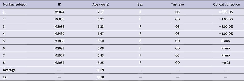
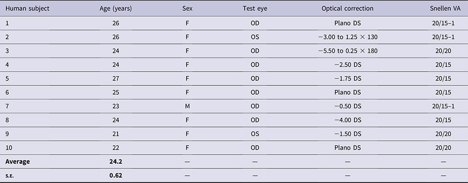
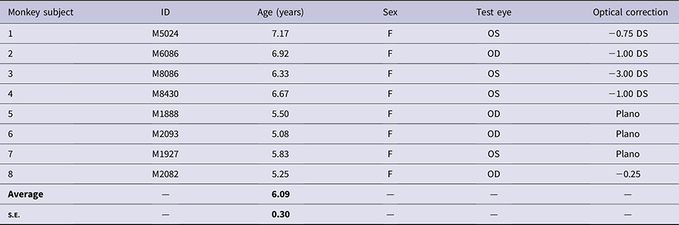
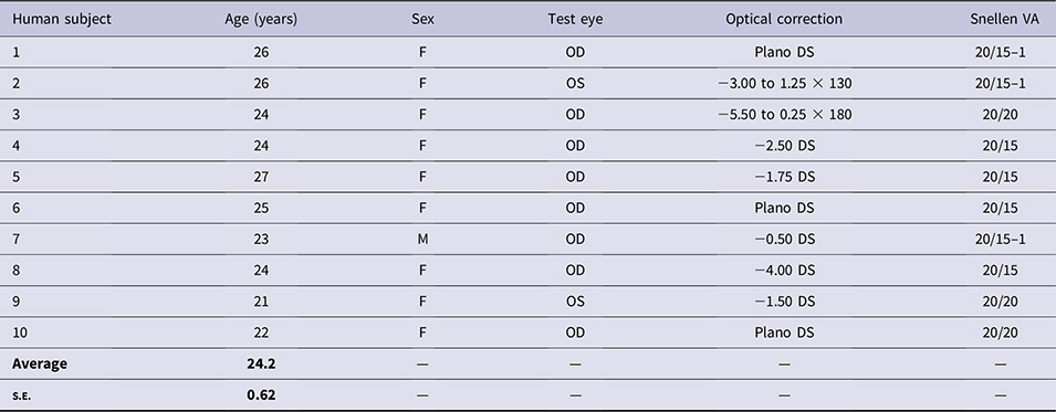
Eight normal, adult crab-eating macaques (Table 1; Macaca fascicularis) and 10 normal, adult humans (Table 2) had their contrast sensitivity measured. Contrast sensitivity measurements were made under monocular conditions. All of the monkeys and 9 of 10 humans were female. The refractive correction used during the measurement of contrast sensitivity is given in the tables. The habitual distance correction was used for the humans.
Demographics for the eight normal Macaca fascicularis used in this study; all testing was done under monocular conditions
Demographics for the 10 normal humans used in this study
The method to determine the lens correction for the monkeys was previously published (Harwerth et al., Reference Harwerth, Smith, Paul, Crawford and von Noorden1991; Wensveen et al., Reference Wensveen, Smith, Hung and Harwerth2011). Initially, retinoscopy was performed on lightly anesthetized (5–10 mg/kg ketamine) and cyclopleged (1–2 drops of 1% cyclopentolate in each eye) monkeys to determine the optical correction for infinity. This optical correction was then adjusted for the contrast sensitivity test distance. Contrast sensitivity was then determined for a 4.6 cpd sine wave grating using lenses in 0.25 diopter steps centered around this adjusted optical correction. The lens correction (Table 1) that gave the highest contrast sensitivity was used in the following experiments.
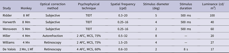
The contrast sensitivity data for M. mulatta and M. nemestrina were obtained from published manuscripts. The Harwerth et al. (Harwerth et al., Reference Harwerth, Smith, Paul, Crawford and von Noorden1991) (8 normal adult M. mulatta) and Wensveen et al. (Wensveen et al., Reference Wensveen, Smith, Hung and Harwerth2011) (5 normal adult M. mulatta) manuscripts used the same methodology used in this study (Table 3). The other studies used different methodology. The study by Miller et al. (Miller et al., Reference Miller, Pasik and Pasik1980) has the contrast sensitivity for four additional M. mulatta. The studies by De Valois et al. (De Valois et al., Reference De Valois, Morgan and Snodderly1974) (adolescent males) and Williams et al. (Williams et al., Reference Williams, Boothe, Kiorpes and Teller1981) (5–18 month old M. nemestrina) have data for six M. nemestrina and one M. fascicularis. Most of the studies did not give the sex of the animals. The stimuli in all of the studies were vertically oriented sine wave gratings.
A comparison of the methods used in six different studies that measured contrast sensitivity in three species of monkey
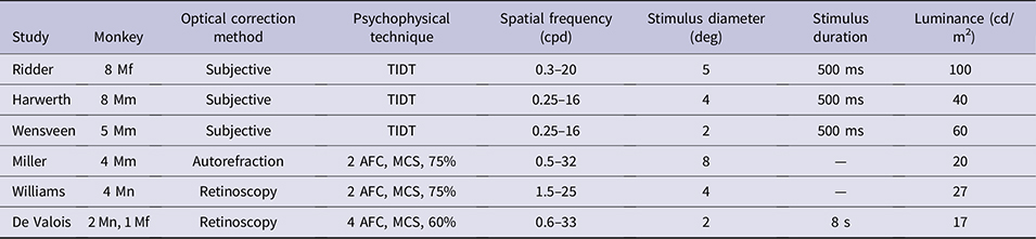
TIDT = temporal-interval detection task; 2 or 4 AFC = 2- or 4-alternative forced choice; MCS = method of constant stimuli; 60% or 75% = percentage taken as threshold on a psychometric function; Mf = M. fascicularis; Mm = M. mulatta; Mn = M. nemestrina.
The monocular contrast sensitivity data were obtained from figures in these published manuscripts using the online app: WebPlotDigitizer (https://automeris.io/WebPlotDigitizer/). The program allows you to upload the published figure. The X and Y axes are calibrated for scale and individual data points can then be highlighted and their coordinates are given.
Stimulus
The stimuli (vertically oriented sine wave gratings overlain with a Gaussian filter) were produced with the Beethoven system (Ryklin Software, Inc., New York, NY). The sine wave gratings were viewed by the monkeys through a 4× reversed telescope on a VPixx monitor (VPixx Technologies, Inc., Saint-Bruno, QC, Canada) at 60 cm. The viewing distance for the humans without the telescope was 200 cm. The average monitor luminance was 100 cd/m2. The sine wave gratings subtended a 5-deg diameter. The stimuli were presented for 500 ms for the monkeys and 1500 ms for the humans.
The monitor was calibrated with a custom program to sequentially render 26 uniformly distributed luminance levels on the VPixx display screen, ranging from RGB (0.0, 0.0, 0.0) black to RGB (255.0, 255.0, 255.0) white. The luminance at each level was measured with a calibrated Cambridge Research Systems (Rochester, Kent, UK) spot photometer (Optical RS232), and the associated software (Lightscan Software Version 3.01). The program saved each luminance level in a lookup table (LUT) accessible by the Beethoven software. The luminance data were used to determine the gamma function (Pelli & Zhang, Reference Pelli and Zhang1991). The gamma value was then utilized to linearize the display intensity output.
Psychophysical procedure
Monkeys
The monkeys were placed in a primate chair (Crist Instrument Co., Inc., Hagerstown, MD) in a sound-isolating chamber (Crist Instrument Co.). The chamber had a white noise generator placed inside to minimize monkey distraction from lab noises. The chair was fit with a drink spout from a liquid reward system (Crist Instruments Co.) for the monkey and a faceplate with two openings for the eyes. Lenses or occluders could be placed over the eye openings.
The monkeys were motivated to perform the psychophysical task through a water restriction program. The water restriction program follows Allergan’s Animal Care and Use Committee (AACUC) fluid regulation policy for NHPs. The minimum amount of water per animal per day was 20 ml per kg. If this amount was not received during the psychophysical procedure, the animal was given the remaining water in their cage at the end of the day. All monkeys were weighed each day using a weight scale placed beneath the primate chair in the sound-isolating chamber (Brecknell Floor Scale, Avery Weigh-Tronix LLC, Fairmont, MN). If the animal lost more than 15% of its baseline body weight, it was removed from the study until it regained weight. Daily food/water consumption, body weight, and general health observations were documented and kept in the animal’s health record, which was available to the veterinary staff.
The psychophysical procedure was identical to that used in previous studies (Harwerth et al., Reference Harwerth, Smith, Boltz, Crawford and von Noorden1983, Reference Harwerth, Smith, Duncan, Crawford and von Noorden1986b, Reference Harwerth, Smith, Paul, Crawford and von Noorden1991; Wensveen et al., Reference Wensveen, Smith, Hung and Harwerth2011). A temporal–interval detection task was used (Table 3). The monkeys were trained to press a response lever when an auditory ready tone (8 Hz) was sounded. This started a trial. They released the lever in response to the stimulus presentation, which occurred randomly from 0.5–6.5 s after the start of the ready tone. A correct response was recorded if the lever was released anytime between 100–900 ms after the start of the stimulus. The monkey was rewarded for a correct response with 0.3 ml of water, a different auditory tone (1.6 KHz), and a 4-s intertrial interval. Releasing the lever before this time interval resulted in a 14-s intertrial interval. If the monkey did not release the lever and the time interval ended, the ready tone ceased indicating the end of the trial. The computer recorded this as a miss by the monkey. The monkey was trained to release the lever when the ready tone ceased. The next trial started in 4 s.
A descending method of limits was used to determine thresholds. Following a correct response by the monkey, the contrast of the next stimulus to be presented was decreased by 0.1 log units. A threshold was defined as the stimulus contrast when two misses in a row were made. After a threshold, the contrast was increased 0.6 log units and the descending method of limits was repeated. Two thresholds were obtained at each spatial frequency during a daily session. The following results gives the average of a minimum of eight thresholds per spatial frequency. Thresholds were obtained for 10 spatial frequencies (0.3–20.2 cpd in 0.2 log unit steps). All experimental procedures were conducted in compliance with the guidelines on animal experimentation set forth by Allergan’s Animal Care and Use Committee (AACUC) and by the Association for Research in Vision and Ophthalmology (ARVO).
Humans
Informed consent was obtained from all subjects after the testing procedure was explained to them and the procedures adhered to the tenets of the Declaration of Helsinki. The procedures were approved by the IRB at Marshal B. Ketchum University. For the human subjects, a chin and forehead rest was placed two meters from the VPixx monitor. The Beethoven system was used. The stimulus was presented for 1500 ms and the subject had 500 ms to respond after the stimulus disappeared. The stimulus diameter was 5 deg. A small white dot was displayed at the center of the VPixx monitor to allow for fixation. The fixation dot disappeared when the stimulus was presented. A descending method of limits was used to determine thresholds. On any given trial, the center of the stimulus was presented one degree to the left or right of fixation (i.e., a 2-alternative forced choice technique). The subject initially determined whether the stimulus was on the left or right of fixation and then responded by pushing a joystick either left or right. The contrast decreased 0.05 log units for each correct response. Threshold was defined as two misses in a row. After a threshold, the contrast increased 0.3 log units and the procedure repeated. A minimum of two thresholds were obtained at each spatial frequency. Contrast sensitivity was determined for eight spatial frequencies (0.75 to 18.5 cpd).
Curve fitting contrast sensitivity functions
The contrast sensitivity functions were fitted with a double exponential function with four floating variables (peak contrast sensitivity, peak spatial frequency, high spatial frequency slope, and low spatial frequency slope) as previously described (Kiorpes et al., Reference Kiorpes, Kiper and Movshon1993; Nusinowitz et al., Reference Nusinowitz, Ridder and Ramirez2007; Ridder & Nusinowitz, Reference Ridder and Nusinowitz2006).
 $${\rm{Contrast}}\;{\rm{sensitivity}} = {K_{\rm{s}}}{\left( {ws} \right)^\alpha }{{\rm{e}}^{ - \beta ws}},$$
where w = spatial frequency, K s = the peak contrast sensitivity of the function, s = the peak spatial frequency of the function, α affects the low spatial frequency slope, and β affects the high spatial frequency slope. All four parameters were allowed to vary freely using an iterative fitting routine in SigmaPlot (Systat Software, Inc., San Jose, CA, Version 12). The area under the curve (AUC) for the contrast sensitivity functions was determined with Excel.
Statistical analysis
A two-sample t-test was used to determine whether the peak contrast sensitivity, peak spatial frequency, AUC, or the extrapolated visual acuity from the contrast sensitivity functions were different between the monkeys and the humans. The statistical analysis was performed with Minitab 16 (Minitab, LLC., State College, Pennsylvania, US; version 16.2.4.0). A comparison of the contrast sensitivity functions from different publications was accomplished with a Kolmogorov–Smirnov goodness of fit test. This was used to determine whether all of the data combined could be thought of as a single sample drawn from a data set.
Results
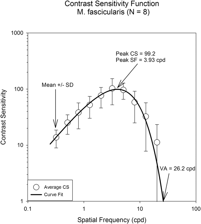
Fig. 1 displays the averaged results for the 8 M. fascicularis from this study. Spatial frequency is plotted on the horizontal axis and contrast sensitivity is plotted on the vertical axis. The open circles represent the mean ± standard deviation for the eight animals. The contrast sensitivity function displays a peak at about 4.0 cpd with a decrease in sensitivity above and below the peak. The solid line drawn through the data is the result of the double exponential curve fit [eqn. (1)]. From the curve fit, the peak contrast sensitivity (99.2) and the spatial frequency (3.93 cpd) at the peak contrast sensitivity were determined (Table 4). The visual acuity (26.2 cpd) was also determined from the curve fit. The visual acuity was taken as the spatial frequency at a contrast sensitivity of one. The AUC was also determined from the curve fit (980.9).
Average contrast sensitivity function for eight Macaca fascicularis. The solid line drawn through the data is the result of the double exponential curve fit [eqn. (1)]. From the curve fit, the peak contrast sensitivity (99.2) and the spatial frequency (3.93 cpd) at the peak contrast sensitivity were determined. The visual acuity (26.2 cpd) was also determined from the curve fit. The AUC was 980.9.

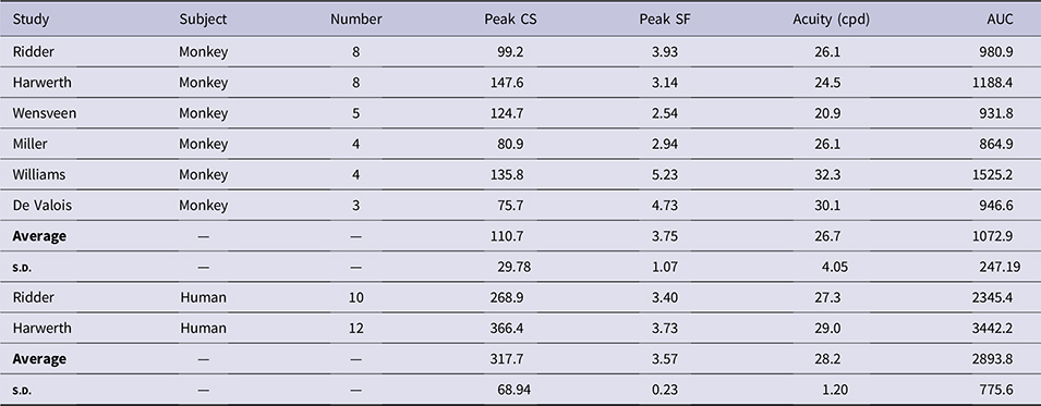
The results of the curve fits [eqn. (1)] to monkey and human data from this study and previously published data. The averaged peak contrast sensitivity and AUC were greater for humans than monkeys. The peak spatial frequency and acuity were not different between the monkeys and the humans
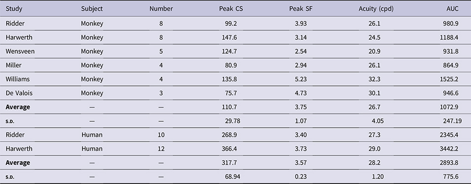
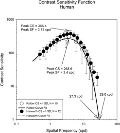
Fig. 2 displays the averaged contrast sensitivity results for the 10 humans from this study (open circles) and 12 humans from Harwerth (filled circles) (Harwerth, Reference Harwerth1982). The figure format is the same as Fig. 1. The solid and the dotted lines drawn through the data represent the result of eqn. (1) for the data from this study and the Harwerth study, respectively. All of the data from the two studies lie within one standard deviation of each other. From the curve fit for the humans from this study, the peak contrast sensitivity was 268.9 and the spatial frequency at the peak contrast sensitivity was 3.4 cpd. The visual acuity (27.3 cpd) and the AUC (2345.4) were also determined from the curve fit (Table 4). For the Harwerth data, the peak contrast sensitivity was 366.4 and the spatial frequency at the peak contrast sensitivity was 3.73 cpd. The visual acuity determined from the curve fit was 29.0 cpd and the AUC was 3442.2.
The averaged contrast sensitivity results for the 10 humans from this study (open circles) and 12 humans from Harwerth (Reference Harwerth1982, filled circles). The solid and the dotted lines drawn through the data represent the result of eqn. (1) for the data from this study and the Harwerth study, respectively. All of the data from the two studies lie within one standard deviation of each other.

The average contrast sensitivity at all spatial frequencies is greater for the human data than the M. fascicularis data (compare Figs. 1 and 2). This resulted in the greater AUC for the humans than the monkeys (Table 4). Curve fits were determined for each of the eight monkeys and the 10 humans from this study. A two-sample t-test indicated that the peak contrast sensitivities [112.0 ± 14.00 (mean ± s.e.) vs. 279.6 ± 37.63; t(11) = 4.37, P = 0.001] and AUC [1128.1 ± 145.79 vs. 2345.4 ± 379.78; t(11) = 3.13, P = 0.010] were statistically significantly lower for the monkeys. The peak spatial frequencies [4.3 ± 0.45 vs. 3.5 ± 0.32; t(12), P = 0.150] and the extrapolated visual acuities [28.7 ± 3.60 vs. 27.3 ± 2.46; t(12) = 0.31, P = 0.763] were not different between the monkeys and the humans.
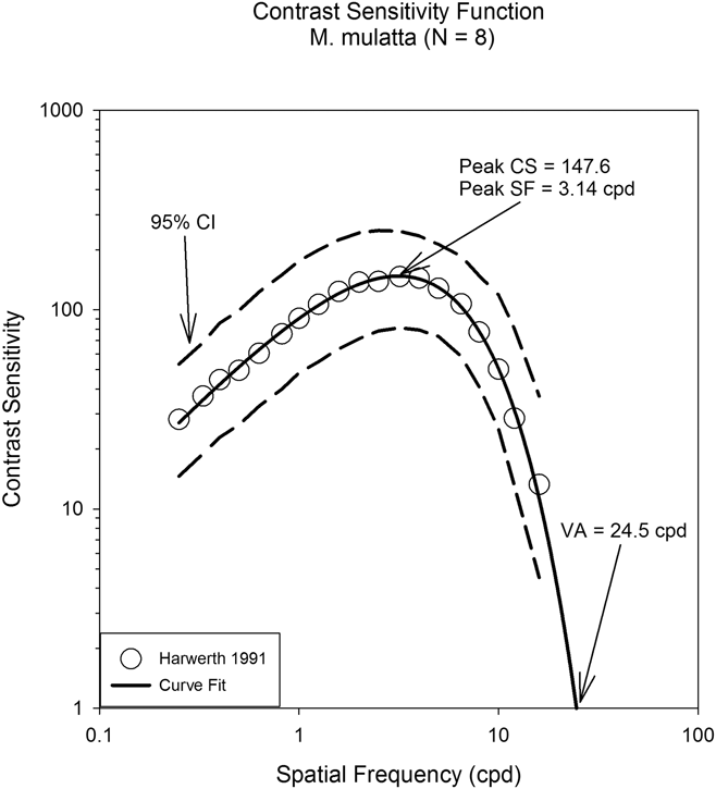
Fig. 3 displays the averaged results for M. mulatta from Harwerth et al. (Harwerth et al., Reference Harwerth, Smith, Paul, Crawford and von Noorden1991). The figure format is the same as Fig. 1. The open circles represent the mean for the eight animals. The solid line drawn through the data is the result of the double exponential curve fit [i.e., eqn. (1)]. From the curve fit, the peak contrast sensitivity (147.6) and the spatial frequency (3.14 cpd) at the peak contrast sensitivity were determined. The visual acuity (24.5 cpd) and the AUC (1188.4) were also determined from the curve fit (Table 4). The dashed lines represent the 95% confidence interval for the data. The contrast sensitivity functions for the M. fascicularis and the M. mulatta (Figs. 1 and 3) appear qualitatively similar. Both functions have a peak around 3–4 cpd and there is a decrease in sensitivity on either side of the peak.
The averaged results for M. mulatta from Harwerth et al. (Reference Harwerth, Smith, Paul, Crawford and von Noorden1991). The open circles represent the mean for the eight animals. The solid line drawn through the data is the result of the double exponential curve fit [i.e., eqn. (1)]. The dashed lines represent the 95% confidence interval for the data.

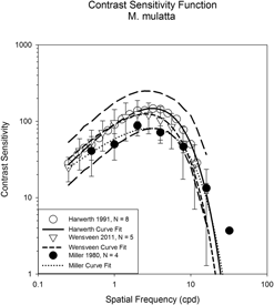
Fig. 4 displays the data from three previously published articles in which the contrast sensitivity was determined for M. mulatta (Miller et al., Reference Miller, Pasik and Pasik1980; Harwerth et al., Reference Harwerth, Smith, Paul, Crawford and von Noorden1991; Wensveen et al., Reference Wensveen, Smith, Hung and Harwerth2011). The data from Harwerth et al. (Harwerth et al., Reference Harwerth, Smith, Paul, Crawford and von Noorden1991) and Wensveen et al. (Wensveen et al., Reference Wensveen, Smith, Hung and Harwerth2011) were collected in the same lab with the same technique (Table 3). These data overlap at all spatial frequencies. The data from Miller et al. (Miller et al., Reference Miller, Pasik and Pasik1980) used a different technique (Table 3). Except for one data point from Miller (i.e., 4.0 cpd), all of the data lies within the 95% confidence interval of the Harwerth (Harwerth et al., Reference Harwerth, Smith, Paul, Crawford and von Noorden1991) data.
The data from three previously published articles in which the contrast sensitivity was determined for M. mulatta. The data from Harwerth et al. (Reference Harwerth, Smith, Paul, Crawford and von Noorden1991) and Wensveen et al. (Reference Wensveen, Smith, Hung and Harwerth2011) were collected in the same lab with the same technique. These data overlap at all spatial frequencies. The data from Miller et al. (Reference Miller, Pasik and Pasik1980) used a different technique. Except for one data point from Miller (i.e., 4.0 cpd), all of the data lies within the 95% confidence interval of the Harwerth data.

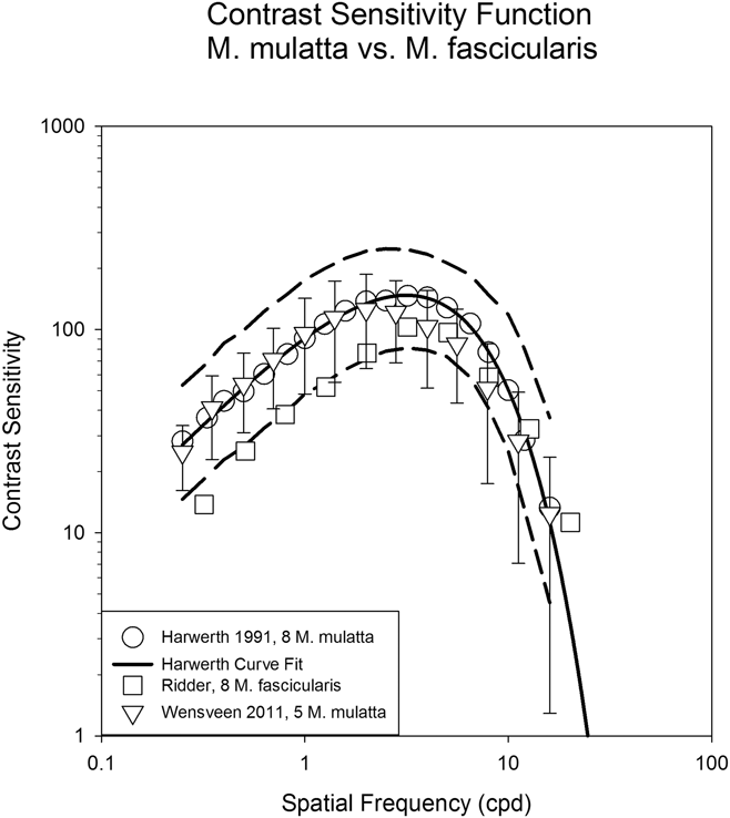
Fig. 5 compares the contrast sensitivity functions for M. mulatta and M. fascicularis using the same psychophysical methods. The data for the M. fascicularis overlay the M. mulatta data for the middle to higher spatial frequencies (above about 3 cpd). For the low spatial frequencies, the M. fascicularis data lie on the lower 95% confidence interval of the M. mulatta data.
The contrast sensitivity functions for M. mulatta and M. fascicularis using the same psychophysical methods. The data for the M. fascicularis overlay the M. mulatta data for the middle to higher spatial frequencies (above about 3 cpd). For the low spatial frequencies, the M. fascicularis data lie on the lower 95% confidence interval of the M. mulatta data.

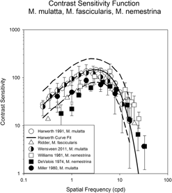
Fig. 6 compares the contrast sensitivity functions for M. mulatta, M. fascicularis, and M. nemestrina. At the higher spatial frequencies (>4 cpd), all of the data lie within the 95% confidence interval of the Harwerth et al. (Reference Harwerth, Smith, Paul, Crawford and von Noorden1991) data. The De Valois et al. (Reference De Valois, Morgan and Snodderly1974) data fall below the 95% confidence interval for the lower spatial frequencies. A Kolmogorov–Smirnov goodness of fit test was used to determine whether there was a significant difference between any of the data sets. Even though the methods used were different for the various studies (Table 3), the test suggests that all of the data could be a single sample from a common distribution (P = 0.24).
The contrast sensitivity functions for M. mulatta, M. fascicularis, and M. nemestrina. At the higher spatial frequencies (>4 cpd), all of the data lie within the 95% confidence interval of the Harwerth et al. (Reference Harwerth, Smith, Paul, Crawford and von Noorden1991) data. The De Valois et al. (Reference De Valois, Morgan and Snodderly1974) data fall below the 95% confidence interval for the lower spatial frequencies. A goodness of fit test suggested that all of the data could be a single sample from a common distribution (P = 0.24).

Discussion
Contrast sensitivity has been measured for many different species using various psychophysical methods (Uhlrich et al., Reference Uhlrich, Essock and Lehmkuhle1981). Uhlrich et al. summarized the contrast sensitivity results for 9 different species (i.e., goldfish, albino rat, hooded rat, cat, pigeon, owl monkey, squirrel monkey, macaque, and human). They found that most of the species (except for the albino and hooded rat) displayed a peak in the contrast sensitivity function with a decrease in sensitivity above and below the peak. By normalizing the contrast sensitivity data, all of the functions overlapped. This suggested that all species have a similar bandpass spatial filter with a peak spatial frequency appropriate for the animals’ visual environment.
The contrast sensitivity functions presented here for monkeys and humans are qualitatively similar to those of other species (Uhlrich et al., Reference Uhlrich, Essock and Lehmkuhle1981). The functions have a peak contrast sensitivity with a decrease in sensitivity on either side of the peak. Contrast sensitivity functions across different species of primates should be similar if the anatomy and physiology of the visual pathways across these species are similar. Previous anatomical and physiological studies of primate visual pathways have indicated that there are similarities between primates but they are not identical (Allman, Reference Allman, Sprague and Epstein1977; Kaas, Reference Kaas, Kaas and Krubitzer2007; Krubitzer, Reference Krubitzer1995; Mountcastle, Reference Mountcastle and Edelman1978; Rockel et al., Reference Rockel, Hiorns and Powell1980; Szentagothai, Reference Szentagothai1975). The comparison presented here of contrast sensitivity across 3 monkey species indicates that they are similar (Fig. 6 and Table 4).
Compared to humans, the contrast sensitivity and the AUC are lower for M. mulatta, M. nemestrina, and M. fascicularis (Table 4). Some of the decrease in sensitivity in the present study may be the result of the different psychophysical methods used for humans and monkeys; however, previous studies (De Valois et al., Reference De Valois, Morgan and Snodderly1974; Harwerth & Smith, Reference Harwerth and Smith1985) used the same methodology for the humans and monkeys and detected the same reduction for monkeys. The peak contrast sensitivity for the humans is about 2.8 times higher than for the monkeys. This agrees with previous studies (Harwerth & Smith, Reference Harwerth and Smith1985; Williams et al., Reference Williams, Boothe, Kiorpes and Teller1981). Similarly, the AUC is 2.7 times greater for the human than the monkeys.
The decreased sensitivity for the monkeys in this study could be the result of a lower monitor luminance. A reversing telescope was used only in the monkey experiments. The screen luminance was measured with and without the reversing telescope. With the telescope, the screen luminance decreased from 100 to 91 cd/m2. The effect of this luminance difference was determined in humans using the same psychophysical technique previously used and a 6.0 cpd stimulus. The average contrast sensitivity for 10 thresholds for 2 subjects was 113 and 95 for the 100 cd/m2 and 91 cd/m2 conditions, respectively. A paired t-test did not indicate these values were different (P = 0.10). Thus, the telescope did reduce the luminance of the monitor, but this did not result in a statistically significant decrease in contrast sensitivity. Furthermore, the studies listed in Table 3 used a range of luminance levels from 17 to 100 cd/m2. The study using the lowest luminance level had the lowest peak contrast sensitivity (De Valois, 75.7) but the study with the highest luminance level did not have the highest peak contrast sensitivity (Ridder, 99.2). Additionally, the Williams study had one of the lowest screen luminance’s (27 cd/m2) but one of the highest peak contrast sensitivities (135.8). Thus, there is not a clear relationship between screen luminance and contrast sensitivity in these studies.
The stimulus duration may also have resulted in lower contrast sensitivities for the monkeys in this study. The stimulus duration for the humans was 1500 ms whereas it was only 500 ms for the monkeys. Temporal integration results in higher sensitivities for longer stimulus durations (Barlow, Reference Barlow1958). However, Fig. 2 demonstrates that the human contrast sensitivity data from this study (stimulus duration 1500 ms) and the Harwerth study (stimulus duration 500 ms) (Harwerth, Reference Harwerth1982) are within one standard deviation of one another and the Harwerth data have a slightly higher sensitivity. Furthermore, the humans and the monkeys in the Harwerth study used the same methodology and stimulus duration (i.e., 500 ms). Thus, the higher contrast sensitivity for the humans in the Harwerth study cannot be the result of differences in stimulus durations.
The peak contrast sensitivity ratio (human/monkey peak contrast sensitivity) for the Harwerth data was 2.48 compared to 2.71 for our data. Thus, the stimulus duration and the threshold method (2 AFC technique in this study vs. temporal–interval detection task in Harwerth study) had little effect on the final contrast sensitivity. The stimulus duration may not have an effect because several studies have demonstrated that the temporal integration time for a contrast detection task is about 200–300 ms, shorter than our stimulus durations (Alexander et al., Reference Alexander, Barnes and Fishman2003; Burr & Santoro, Reference Burr and Santoro2001). Thus, regardless of the methods used, several species of monkey exhibit a decrease in contrast sensitivity compared to humans.
Some studies comparing contrast sensitivity between humans and one species of monkey have suggested that the visual acuity of the monkey is lower than that of the human (De Valois et al., Reference De Valois, Morgan and Snodderly1974; Harwerth & Smith, Reference Harwerth and Smith1985). The average of several studies (Table 4) suggests that the spatial frequency at the peak (3.75 ± 1.07 vs. 3.57 ± 0.23) and the acuities (26.7 ± 4.05 vs. 28.2 ± 1.20) are similar between nonhuman and human primates. This occurred because the high spatial frequency slope of the contrast sensitivity curve fit was steeper for the humans than the monkeys. The main reason previously given for the lower acuity in monkeys is the smaller eyes of monkeys that result in less optical magnification. The axial length of normal adult monkeys can vary from 16.40 ± 0.10 mm to 20.24 ± 1.03 mm (Fernandes et al., Reference Fernandes, Bradley, Tigges, Tigges and Herndon2003; Wiesel & Raviola, Reference Wiesel and Raviola1979). The axial length is affected by the species, sex, and age of the animal. The axial length for middle aged humans is about 23.5 mm (Meng et al., Reference Meng, Butterworth, Malecaze and Calvas2011). Thus, in general, the axial lengths of monkey eyes are shorter than humans but there is a high variability. The averaged data presented here do not suggest that monkeys (26.7 ± 4.05 cpd) have a significantly lower acuity than humans (28.2 ± 1.20 cpd).
Since the 3 species of macaque examined in this study are evolutionarily more closely related than they are to humans, the contrast sensitivity functions of these monkeys should be more similar to each other than to human. A goodness of fit test for the monkey results suggested that all of the data could be a single sample from a common distribution. However, there were some differences in the shape of the function between the three species. For example, the De Valois data had low contrast sensitivities for low spatial frequencies (Fig. 6). The difference in the psychophysical methods that De Valois used could not account for the decrease in sensitivity at only low spatial frequencies (Table 3). His psychophysical technique would have affected all spatial frequencies equally. Similarly, the low stimulus luminance De Valois used would not have produced the decrease in sensitivity only at low spatial frequencies. As the luminance of the stimulus is decreased, the overall contrast sensitivity decreases, the peak of the function shifts to lower spatial frequencies, and the low spatial frequency falloff decreases (van Nes et al., Reference van Nes, Koenderink, Nas and Bouman1967; De Valois et al., Reference De Valois, Morgan and Snodderly1974). Uncorrected refractive errors could also not be the cause (Table 3). An increase in the uncorrected refractive error causes the same change in the contrast sensitivity function that decreasing the stimulus luminance causes (Williams & Boothe, Reference Williams and Boothe1983). However, the decreased sensitivity may have occurred because the stimulus diameter used by De Valois was only 2 deg (Table 3). This would result in only a few cycles of the stimulus being visible for the low spatial frequencies. Previous studies have indicated that the contrast sensitivity increases as the visible stimulus cycles increase (McCann et al., Reference McCann, Savoy, Hall and Scarpetti1974; Robson & Graham, Reference Robson and Graham1981). However, Wensveen also used a stimulus diameter of 2 deg and their data do not show a decrease in sensitivity at low spatial frequencies (Fig. 6 and Table 3).
The high spatial frequency data from Williams and De Valois for M. nemestrina have contrast sensitivities higher than most of the other data. The M. nemestrina curve fits also have higher peak spatial frequencies and higher extrapolated visual acuities than the other species. This suggests that the functions for the M. nemestrina may be shifted to higher spatial frequencies than that for the M. mulatta and M. fascicularis. This shift in the function cannot be explained by their psychophysical methodology or the age of the monkeys. Williams and De Valois used adolescent monkeys whereas the other studies used adults. Younger animals, that have not reached maturity, would have functions shifted to lower spatial frequencies. It is possible that the shift in the function is the result of the fewer animals used in their studies (N = 3 or 4) compared to the other monkey studies (N = 8). With fewer subjects, intersubject variability could have a greater effect on the average contrast sensitivity.
In conclusion, this study demonstrates that the contrast sensitivity functions for M. mulatta, M. nemestrina, and M. fascicularis are similar even though different methods were used. Thus, previous contrast sensitivity results for experimentally induced amblyopia and/or glaucoma can be compared across these different NHP species. The contrast sensitivity functions for the NHPs had lower peak contrast sensitivities and AUCs than the humans. The peak spatial frequency and visual acuity extrapolations were the same for the humans and the NHPs. The contrast sensitivity differences and similarities between humans and NHPs should be considered when using NHPs to study human visual diseases.
Conflict of interest
The authors declare no competing financial interests.