
1. Introduction
The sedimentation of heavy particles is a commonly observed phenomenon in both nature and engineering applications. Accurately predicting the settling velocity of particles in viscous fluids is essential in many fields that are not limited to soil preservation, particulate matter control, fluidized beds design and COVID-19 transmission containment (Balachandar & Eaton Reference Balachandar and Eaton2010; Bourouiba Reference Bourouiba2021). In the simplest scenario of a spherical particle settling in quiescent fluid, the particle reaches its terminal velocity when the gravitational force is balanced by the buoyancy force and the particle drag. The terminal velocity can be explicitly computed from the balance. When the surrounding flow is turbulent, however, the prediction of the terminal settling velocity becomes a lot more complex. Not only do the mechanisms of turbulence affecting particle sedimentation need further exploration, but models to predict the particle settling speed in turbulent flows are also under development.
Most of the previous efforts to understand the influence of turbulence on the particle settling speed were devoted to point particles whose sizes are negligible compared with the size of the turbulent eddies. Depending on the particle and fluid parameters, both enhanced and reduced terminal velocities can be observed (Good et al. Reference Good, Ireland, Bewley, Bodenschatz, Collins and Warhaft2014; Rosa et al. Reference Rosa, Parishani, Ayala and Wang2016). When the inertia is small, particles tend to ride on the downward flow side of vortices in a turbulent field and reach a higher settling speed than their counterparts in laminar flows (Wang & Maxey Reference Wang and Maxey1993). This phenomenon is now known as ‘preferential sweeping’, which has been widely observed in both experiments and numerical simulations (e.g. Wang & Maxey Reference Wang and Maxey1993; Yang & Lei Reference Yang and Lei1998; Aliseda et al. Reference Aliseda, Cartellier, Hainaux and Lasheras2002; Yang & Shy Reference Yang and Shy2003). With greater particle inertia, reductions in the settling speed in turbulent fields can also be observed. The primary mechanism contributing to these reductions is ‘loitering’, which refers to the fact that particles stay statistically longer in the upward flow regions than in the downward flow regions (Nielsen Reference Nielsen1993). The loitering is closely related to the nonlinear drag under finite particle Reynolds numbers. In direct numerical simulations, the reductions in the particle settling speed were observed only when the nonlinear drag correction was considered (Good et al. Reference Good, Ireland, Bewley, Bodenschatz, Collins and Warhaft2014). Through a series of experimental and direct numerical simulations, Good et al. (Reference Good, Ireland, Bewley, Bodenschatz, Collins and Warhaft2014) concluded that the settling number  $\tau _pg/u'$, where
 $\tau _p$ is the particle response time,
 $g$ is the gravitational acceleration and
 $u'$ is the turbulent root-mean-square (r.m.s.) velocity, is a crucial parameter to predict enhancements or reductions of the particle settling speed due to turbulence. For particles with finite Reynolds numbers, the settling speed can be accelerated by turbulence when the settling number is above unity. Otherwise, deceleration of the settling speed should still be expected (Good et al. Reference Good, Ireland, Bewley, Bodenschatz, Collins and Warhaft2014). Aside from homogeneous isotropic turbulence (HIT), there are some recent efforts to extend the investigations of the turbulence effect on the settling speed of inertial particles to more realistic wall-bounded turbulence (e.g. Lee & Lee Reference Lee and Lee2019; Bragg, Richter & Wang Reference Bragg, Richter and Wang2021). Compared with HIT, the non-zero shear rate of the mean flow, the non-uniform distribution of turbulent kinetic energy and the anisotropic near-wall flow structures in the wall-bounded turbulence could all greatly complicate the picture of turbulence–particle interactions. Generalizing mechanisms and control parameters for the turbulent effect on the particle settling speed becomes much more difficult.
With the developments of experimental techniques and interface-resolved direct numerical simulations (IR-DNSs), investigations of the particles settling speed in turbulent environments have been successfully extended to finite-size particles (e.g. Byron Reference Byron2015; Fornari, Picano & Brandt Reference Fornari, Picano and Brandt2016a; Fornari et al. Reference Fornari, Picano, Sardina and Brandt2016b; Chouippe & Uhlmann Reference Chouippe and Uhlmann2019). Here, finite-size particles refer to particles whose diameters are comparable to or larger than the Kolmogorov length in turbulence that could introduce significant disruptions, distortions and discontinuity to the flow field (Eaton Reference Eaton2009). Unlike point particle cases, turbulence seems to consistently reduce the settling speed of finite-size particles. Byron (Reference Byron2015) found that when the size of the particle was comparable to the Taylor microscale of a HIT, the settling speed was reduced by 40 % to 60 % due to turbulence with a settling number around unity. These reductions were much higher than those reported by Good et al. (Reference Good, Ireland, Bewley, Bodenschatz, Collins and Warhaft2014) with similar settling numbers. Fornari et al. (Reference Fornari, Picano and Brandt2016a) simulated sedimentation of individual and multiple particles in a quiescent fluid and HIT. The average settling speed of multiple particles was 4 % below its counterpart associated with individual particles in quiescent fluid and 12 % in HIT. These reductions were attributed to the hindering effect, which means that, when a large number of finite-size particles settle downwards, the fluid is pushed upwards due to the incompressibility of the flow field, and this upward moving fluid would hinder the sedimentation of particles (Yin & Koch Reference Yin and Koch2007). Fornari et al. (Reference Fornari, Picano, Sardina and Brandt2016b) also investigated the influences of the Galileo number, a non-dimensional number measuring the relative importance of the gravitational force and viscous force, and the particle volume fraction on the settling speed of finite-size particles in HIT. More significant reductions in the settling speed were observed in cases with more intense turbulence and less-heavy particles. Fornari et al. (Reference Fornari, Picano, Sardina and Brandt2016b) explained this phenomenon as an effect of nonlinear particle drag. Particles with moderate density ratios in turbulence could yield more significant motions relative to their ambient fluids in the plane perpendicular to the settling direction. These relative motions eventually enhanced the drag force due to its nonlinear dependence on the relative velocity. Chouippe & Uhlmann (Reference Chouippe and Uhlmann2019) investigated the settling of large numbers of particles in a HIT using direct numerical simulations in large computational domains. They found that when the particle volume fraction increased, the turbulent effect became weaker, while the hindering effect and the particle interactions dominated the settling speed. Due to particle aggregation and conglomeration, the settling speed of a large group of particles could surpass its counterpart for individual particles (Chouippe & Uhlmann Reference Chouippe and Uhlmann2019). Due to the complexity of the interactions between the turbulent carrier flows and the dispersed particle phases, there are still significant gaps to overcome before the general principles of turbulent effects on the settling speed of finite-size particles can be generalized.
In order to reach a better understanding of how turbulence modifies the settling speed of finite-size particles, it is crucial to answer questions such as how the mean drag coefficient of a particle changes in turbulent environments and what mechanisms are responsible for this modification. Most of the studies to address the first question were conducted through experiments, and their focused particle Reynolds numbers were mainly above the critical point, i.e. the Reynolds number at which the particle drag coefficient experiences a sudden jump (Torobin & Gauvin Reference Torobin and Gauvin1961; Clamen & Gauvin Reference Clamen and Gauvin1969). These experimental studies generally reported forward-shifted critical points due to turbulence, but the efforts of modelling the particle drag coefficients in turbulence seemed to conflict with each other, as summarized in Crowe et al. (Reference Crowe, Schwarzkopf, Sommerfeld and Tsuji2011, Chap. 4). For moderate particle Reynolds numbers, the only experimental effort to model the drag coefficient in turbulence was contributed by Uhlherr & Sinclair (Reference Uhlherr and Sinclair1971), who predicted linearly increased drag coefficients with the turbulence intensity.
Besides experimental studies, DNSs were also employed to generate data and build reliable models to predict particle drag in turbulence (Bagchi & Balachandar Reference Bagchi and Balachandar2003; Homann, Bec & Grauer Reference Homann, Bec and Grauer2013). Due to the Reynolds number constraints, those studies focused on moderate particle Reynolds numbers much lower than the critical points. Bagchi & Balachandar (Reference Bagchi and Balachandar2003) conducted DNS for the case of frozen free-stream turbulence passing over fixed particles. The diameters of the particles were 1.5 to 10 times the Kolmogorov length, and the turbulence intensity was between 10 % and 25 %. It was reported that turbulence had little effect on the time-averaged drag coefficient, and the standard drag correlation was sufficient to predict the drag force. Homann et al. (Reference Homann, Bec and Grauer2013), on the other hand, measured the drag forces on the particles in real-time HIT superposed with a constant velocity. It was found that, even considering the nonlinear drag effect, the standard drag correlation still significantly underestimated the time-averaged drag forces. Aside from these conflicting overall observations in the literature, the mechanisms through which turbulence modifies the mean drag force are also not fully clear. Homann et al. (Reference Homann, Bec and Grauer2013) attributed their observed particle drag enhancements to the interactions between the small-scale turbulent eddies and the particle boundary layer, but more details on these interactions are yet to be revealed.
In this work, we use IR-DNSs based on the lattice Boltzmann approach to investigate the overall effects of turbulence on the mean particle drag and the associated mechanisms. Unlike the study of Homann et al. (Reference Homann, Bec and Grauer2013), where the particles were directly placed in HIT, a different physical setting of free-streaming turbulence passing over the fixed particles is adopted. The remaining article is structured as follows. The flow configuration and the numerical approach are introduced in § 2. Then, a grid-independence study is reported in § 3 to serve validation purposes and to find the optimal mesh that balances the computational cost and numerical accuracy. Through systematic comparisons of the particle drag in laminar and turbulent flows, the modifications of the particle drag due to turbulence are discussed in § 4, and the associated mechanisms are analysed. Models are also proposed to quantify the mean drag of individual particles and particle arrays in turbulent flows. Finally, the main conclusions of the present work are given in § 5.
2. Problem description and numerical method
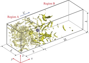
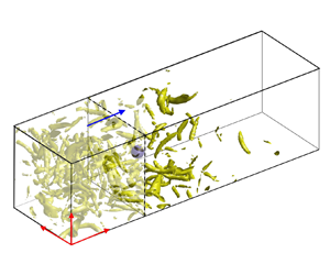
In the previous study of Homann et al. (Reference Homann, Bec and Grauer2013), HIT was generated in a cuboid domain with a superposed mean flow speed, and the particle was placed directly in the flow. In the present study, however, a different flow configuration is adopted. As shown in figure 1, a computational domain with a size of  $L_x\times L_y\times L_z = 3L\times L \times L$ is divided into two regions, region A and region B. Region A is a periodic cube with a size of
 $L^3$, where HIT with different intensities is generated. Region B is a cuboid domain of
 $2L\times L \times L$ with an inlet, an outlet and four periodic sides, where the fixed particle or particle array confronts the incoming turbulent flow. The time-dependent velocity field on a given slide of region A is abstracted and superposed with a constant velocity
 $U$ to define the velocity at the inlet of region B. A convective condition of
 $\partial {\boldsymbol {u}}/\partial t + U_{out}\partial {\boldsymbol {u}}/\partial x = 0$ is given to the outlet of region B, where
 $U_{out}$ is the local streamwise velocity. A particle with a diameter
 $d_p$ is placed at the centre of the
 $y$–
 $z$ plane
 $2d_p$ away from the inlet, i.e.
 ${\boldsymbol {x}}_c = (L+2d_p,L/2,L/2)$, where
 ${\boldsymbol {x}}_c$ is the particle centre. As shown later in table 1, the distance from the particle to the inlet of region B is roughly equal to the longitudinal integral length scale of the HIT generated in region A. A similar configuration was also adopted in some previous studies, such as those of Xu & Subramaniam (Reference Xu and Subramaniam2010) and Botto & Prosperetti (Reference Botto and Prosperetti2012).
The configuration of the flow studied in the present study.

Statistics of HIT. The LBM results are converted from the LB units, i.e.  $\Delta x_{LBM} = 1$,
 $\Delta t_{LBM} = 1$ to the spectral units of
 $L_{spectral} = 2{\rm \pi}$ and
 $\Delta t_{spectral} = 0.00004$ to make direct comparisons with the benchmark results from the PS simulation. Unless otherwise specified, the results are presented in spectral units throughout the entire article.

Unlike the Homann et al. (Reference Homann, Bec and Grauer2013) setting, the current setting isolates the particle from its wake. Although Homann et al. (Reference Homann, Bec and Grauer2013) showed that the mean flow speed after the particle was quickly restored within a short distance, this study does not fully eliminate the chance of the particle meeting its wake due to the periodic boundary condition in the streamwise direction. Some vortices generated from the particle surface could be very persistent and require a very extended period to decay. In a study on the sensitivity of the turbulent statistics on the pipe length by Chin et al. (Reference Chin, Ooi, Marusic and Blackburn2010), it was reported that the periodic boundary effects on the high-order turbulent statistics needed a pipe length up to 18.5 times the pipe diameter to decay completely. Another potential issue of directly placing a finite-size particle in HIT is that the flow around the particle could be significantly disturbed (Eaton Reference Eaton2009; Vreman Reference Vreman2016), so the statistics of HIT may not describe the turbulent flow seen by the particle accurately. Moreover, Lucci, Ferrante & Elghobashi (Reference Lucci, Ferrante and Elghobashi2010) argued that finite-size particles in a forced HIT could interfere with the large-scale forcing to sustain turbulence, which was usually based on a continuous flow field, and led to inevitable inaccuracy. Although the current configuration does not have the above issues, once the HIT enters region B its intensity decays, and the isotropy is no longer maintained. To accurately capture the information of the turbulent flow seen by the particle, additional simulations of the corresponding unladen cases are needed.
The numerical simulations in the present study are conducted by the lattice Boltzmann method (LBM) with interpolated bounce-back (IBB) schemes to treat the no-slip condition on the particle surface. This method was the same one used in our previous studies on particle-laden turbulent channel and pipe flows (Peng, Ayala & Wang Reference Peng, Ayala and Wang2019c; Peng & Wang Reference Peng and Wang2019). The flow solver adopts a multi-relaxation time model based on a D3Q27 lattice grid, i.e. three-dimensional lattice grid with 27 velocities. The inlet boundary condition of region B with given velocity fields is realized by the half-way bounce-back scheme (Ladd Reference Ladd1994), while the outlet boundary is treated with the scheme proposed by Lou, Guo & Shi (Reference Lou, Guo and Shi2013). The LBM can be incorporated with both IBB schemes and the immersed boundary methods (IBM) to handle the no-slip boundary treatment in complex geometries. Both approaches have been successfully applied to particle-laden turbulent flows with IBB (e.g. Gao, Li & Wang Reference Gao, Li and Wang2013; Jebakumar, Magi & Abraham Reference Jebakumar, Magi and Abraham2018) and with IBM (Ten Cate et al. Reference Ten Cate, Derksen, Portela and Van Den Akker2004; Rubinstein, Derksen & Sundaresan Reference Rubinstein, Derksen and Sundaresan2016; Eshghinejadfard et al. Reference Eshghinejadfard, Abdelsamie, Hosseini and Thévenin2017). We conducted systematic comparisons between these two approaches in both laminar and turbulent cases (Peng et al. Reference Peng, Ayala, Brändle de Motta and Wang2019a; Peng, Ayala & Wang Reference Peng, Ayala and Wang2019b). These studies confirmed that IBB schemes not only ensured second-order accurate velocity fields but also led to much smaller numerical errors in the results of the fluid velocity, hydrodynamic force/torque and turbulent dissipation rate. On the other hand, IBM possessed better numerical stability and resulted in weaker artificial fluctuations in the results of instantaneous force/torque for moving particles. It should also be pointed out that, while the fluid velocity was only first-order accurate with IBM, the integrated force/torque of the particles may still be second-order accurate, as reported in the literature (e.g. Breugem Reference Breugem2012) and confirmed by our own simulation results (Peng et al. Reference Peng, Ayala and Wang2019b). Since particles are static in the present study, IBB schemes are more suitable for the no-slip boundary treatment on the particle surfaces. The quadratic IBB scheme by Bouzidi, Firdaouss & Lallemand (Reference Bouzidi, Firdaouss and Lallemand2001) is adopted.
In the study of Homann et al. (Reference Homann, Bec and Grauer2013), the flow field was solved by a pseudo-spectral method, and the no-slip boundary condition was treated with IBM. This combination resulted in a 1.5-order error convergence rate for the particle drag, which is lower than the second-order error convergence rate with the present approach (Peng et al. Reference Peng, Ayala and Wang2019b). It should be pointed out that our convergence rate was calculated using the numerical results with the highest grid resolution of  $d_p/\Delta x = 48$ as the benchmark results, while the convergence rate reported by Homann et al. (Reference Homann, Bec and Grauer2013) used the Schiller & Naumann correlation (Schiller & Naumann Reference Schiller and Naumann1933) as their benchmark results:
 \begin{equation} C_{D}^{SN} = \frac{24}{Re_p}(1 + 0.15Re_p^{0.687}), \end{equation}
where  $Re_p = Ud_p/\nu$ is the particle Reynolds number, and
 $\nu$ is kinematic viscosity. For more information on the numerical approach used in the present study, readers can refer to our previous publications (e.g. Peng Reference Peng2018; Peng et al. Reference Peng, Geneva, Guo and Wang2018).
3. The parameter settings and the grid-independence study
The numerical approach used in this study has been validated thoroughly through multiple test cases, including those in the laminar and turbulent regimes, laden and unladen with particles (Peng Reference Peng2018; Brändle de Motta et al. Reference Brändle de Motta2019). Therefore, further validation of the approach itself is not performed. Here, we conduct a grid-independence study to ensure that the grid meshes used in numerical simulations are sufficient to resolve the turbulent flows and capture the force acting on particles.
The HIT in region A is generated with the stochastic forcing model of Eswaran & Pope (Reference Eswaran and Pope1988). The estimated rate of the energy input, whose time average is equal to the averaged dissipation rate  $\langle \epsilon \rangle$ is
 \begin{equation} \langle \varepsilon \rangle = \frac{4N_f\sigma_f^2T_f}{1+T_f(\sigma_f^2T_f N_f k_0^2)^{1/3}\beta}, \end{equation}
where  $N_f$ is the number of total force modes,
 $\sigma _f^2$ is the forcing magnitude,
 $T_f$ is the forcing time scale,
 $k_0 = 1$ is the lowest normalized wavenumber, i.e.
 $k_0 = L/l_0$,
 $l_0$ is the longest wavelength, and
 $\beta = 0.8$ is a fitting parameter in the model. In this stochastic forcing model, only the large-scale flow structures whose wavenumbers satisfy
 $0 < |{\boldsymbol {k}}| < 8$ are forced, corresponding to a total of 80 forced modes. We adjust the values of
 $\sigma _f^2$ and
 $T_f$ to generate turbulent flows with different intensities, and this information is summarized in table 1. Rosa et al. (Reference Rosa, Parishani, Ayala and Wang2015) systematically examined the parameterizations for this stochastic forcing model and showed that, when the ratio between the forcing time scale
 $T_f$ and the Kolmogorov time scale was small, (3.1) yielded reasonable estimations of the dissipation rate in the generated turbulent fields.
To demonstrate that the background HIT in region A is well resolved, simulations with two grid meshes, i.e.  $256^3$ and
 $512^3$, are conducted. Five background turbulence (BT) levels, labelled from BT1 to BT5 from weak to strong are generated, and their statistics after the flow reached statistical stationary states are tabulated in table 1. These statistics include: the turbulent kinetic energy (TKE)
 $\langle E\rangle$, where
 $\langle \cdots \rangle$ represents ensemble averaging unless otherwise specified, the r.m.s. velocity of a single velocity component
 $\langle u'\rangle$, the dissipation rate of TKE
 $\langle \varepsilon \rangle = 2\nu \langle s'_{ij}s'_{ij}\rangle$, where
 $s'_{ij}$ is the fluctuation part of the strain rate tensor, the longitudinal integral length scale,
 $\langle l \rangle$, the Reynolds number
 $\langle Re_\lambda \rangle = \langle u'\lambda /\nu \rangle$ based on the Taylor microscale
 $\lambda = \sqrt {15\nu u'^2/\varepsilon }$, the Kolmogorov length
 $\langle \eta \rangle$, the skewness
 $\langle S\rangle$ and flatness
 $\langle F\rangle$ of the longitudinal velocity gradients,
 \begin{equation}
\left\langle S\right\rangle =
\frac{\left\langle \frac{1}{3}(s_{xx}^{\prime3}+s_{yy}^{\prime3}+s_{zz}^{\prime3})\right\rangle}{\left\langle \frac{1}{3}(s_{xx}^{\prime2}+s_{yy}^{\prime2}+s_{zz}^{\prime2})\right\rangle^{1.5}},\quad
\left\langle F\right\rangle = \frac{\left\langle \frac{1}{3}(s_{xx}^{\prime4}+s_{yy}^{\prime4}+s_{zz}^{\prime4})\right\rangle}{\left\langle \frac{1}{3}(s_{xx}^{\prime2}+s_{yy}^{\prime2}+s_{zz}^{\prime2})\right\rangle^{2}},
\end{equation}
and the eddy turnover time  $\langle T_e\rangle = \langle u'^2/\varepsilon \rangle$. The uncertainties of the statistics in table 1 are computed as the standard deviation of the averaged quantities, i.e.
 \begin{equation} \sigma_{\bar{A}} = \sigma_{A}\sqrt{\frac{2T_c}{\Delta T_{ave}}}, \end{equation}
where  $\sigma _A$ is the standard deviation of time-dependent quantity
 $A(t)$,
 $T_c$ is the correlation time of
 $A(t)$ and
 $\Delta T_{ave}$ is the duration of the statistical averaging. The correlation time
 $T_c$ is obtained from the coefficient
 $R(\tau ) \equiv \langle A(t_1)A(t_1 + \tau )\rangle /\sigma _A^2$ for
 $R(T_c) = 0.5$ (Wang et al. Reference Wang, Ayala, Gao, Andersen and Mathews2014).
For conciseness, the statistics from the high-resolution simulations of  $512^3$ are only shown for BT5 with the greatest
 $\langle Re_\lambda \rangle$, which demands the highest grid resolution. The benchmark data from our in-house pseudo-spectral (PS) code are also included for comparison. As shown in table 1, the turbulent statistics are already well predicted with the grid mesh of
 $256^3$, even for the sensitive high-order statistics
 $\langle S\rangle$ and
 $\langle F\rangle$. In our previous comparative study between LBM and the PS method on simulating the forced single-phase HIT, it was found that the simulation with the second-order accurate LBM roughly needed doubled grid resolutions compared with the PS simulation at moderate
 $Re_\lambda$. This roughly sets the grid resolution requirement for LBM
 $\langle k_{max}\eta \rangle > 2$ (Wang et al. Reference Wang, Ayala, Gao, Andersen and Mathews2014), where
 $k_{max} = N/2$ is the maximum wavenumber and
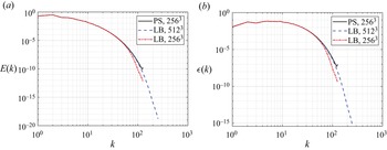
 $N$ is the number of grid mesh points in each direction. This statement is also supported by the comparisons of TKE and dissipation rate spectra of BT5 in figure 2. The LBM results with the mesh of
 $512^3$ collapse perfectly with the PS results with half the mesh size (2563). When the mesh sizes are both
 $256^2$, LBM resolves flow scales of
 $k < k_{max}/2 = 64$ quite well but underestimates the TKE for smaller scales. As a compromise in considering the numerical accuracy and the computational cost, a consistent grid mesh of
 $256^3$ is adopted in this study to generate the background HIT.
The TKE and dissipation rate spectra of the background HIT.

It is equally important to represent the particle with sufficient grid numbers in particle-laden turbulent flow simulations so that the force/torque on the particle can be accurately assessed. In order to find this sufficient grid resolution, simulations of a fixed particle in uniform incoming flows are conducted at different particle Reynolds numbers. These simulations are conducted in a domain of  $20d_p\times 10d_p\times 10d_p$ that has the same boundary conditions as region B. The particle is fixed at
 $(5d_p,5d_p,5d_p)$ and the grid resolutions, i.e.
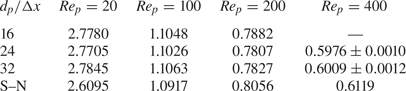
 $d_p/\Delta x$ are varied. The drag coefficient results in these simulations are compiled in table 2. For
 $Re_p$ ranging from 20 to 400, a grid resolution of
 $d_p/\Delta x = 24$ is sufficient to capture the drag force acting on the particle accurately. The empirical results predicted by the Schiller–Naumann correlation (Schiller & Naumann Reference Schiller and Naumann1933) are presented as references in table 2. However, these results should not be regarded as the benchmark for quantitative assessments since the numerical settings in the simulations, such as the domain size and boundary conditions, are not precisely identical to Schiller & Naumann's experimental study. It is interesting to observe that the converged drag coefficients for
 $Re \leqslant 100$ are 6.7 % to 1.3 % larger than the corresponding value from the Schiller–Naumann correlation, whereas those for
 $Re \geqslant 200$ are 1.8 % to 2.8 % less than the corresponding value from the Schiller–Naumann correlation. The former is likely due to the confinement effect of the domain size. The reason for the latter could be partially due to the fitting error of the Schiller–Naumann correlation.
The comparison of particle drag coefficients with different grid resolutions in the case of laminar flows passing over a fixed sphere.

One of the key advantages of the flow configuration adopted in the present study compared with its counterpart in Homann et al. (Reference Homann, Bec and Grauer2013) is that the particle wake would not re-enter the computational domain. However, we still need to ensure that the size of the computational domain is sufficiently large so that the simulation results are not affected by the treatment of the outflow boundary condition. To confirm this, we compare the drag coefficients on a fixed particle in uniform flows with two domain lengths,  $20d_p\times 10d_p\times 10d_p$ and
 $30d_p\times 10d_p\times 10d_p$. The particle in both domains is fixed at
 $(5d_p,5d_p,5d_p)$. As shown in table 3, a domain length of
 $20d_p\times 10d_p\times 10d_p$ is sufficient to ensure that the convective outflow boundary treatment does not alter the drag force on the particle.
The comparison of particle drag coefficients with different domain length in the case of laminar flows passing over a fixed sphere.

The simulations of free-streaming turbulence passing over a fixed particle and particle arrays are based on the five background HITs (BT1 to BT5 in table 1) with  $Re_\lambda$ ranging from 24 to 63. Three particle Reynolds numbers,
 $Re_p = 100$, 240 and 330, defined with the mean flow velocity
 $U$ are selected. These Reynolds numbers are chosen to correspond to three regimes of wake formats, i.e. the steady axisymmetric regime with
 $20 < Re_p < 210$, the steady planar-symmetric regime with
 $210 < Re_p < 270$ and the unsteady planar-symmetric regime with
 $270 < Re_p < 400$ with uniform incoming flows (Jones & Clarke Reference Jones and Clarke2008; Ern et al. Reference Ern, Risso, Fabre and Magnaudet2012). It should be noted that the precise particle Reynolds numbers for the wake to switch from one regime to another vary in the literature. Therefore, particle Reynolds numbers are chosen around the middle point in each range to ensure that three wake regimes are indeed covered. For validation purposes, we simulated the case of uniform flow passing over a fixed sphere in each wake regime using a domain size of
 $20d_p\times 10d_p\times 10d_p$, with a grid size of
 $d_p/\Delta x = 24$. The vortex structures visualized by the
 $Q$-criterion (
 $Q = 0.5(\omega_{ij}\omega_{ij} - s_{ij}s_{ij})$, where
 $\omega_{ij}$ and
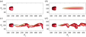
 $s_{ij}$ are the anti-symmetric and symmetric parts of the velocity gradient tensor, respectively) in the particle wake are compared in figure 3. Correct vortex structures are successfully captured in each wake regime.
The wake structures visualized by the  $Q$-criterion in different wake regimes: (a)
 $Re_p = 200$, steady axisymmetric wake; (b)
 $Re_p = 240$, steady planar symmetric wake; (c)
 $Re_p = 330$, unsteady planar symmetric wake; and (d)
 $Re_p = 420$, three-dimensional chaotic wake. The colour on the isosurface represents the streamwise velocity.

Based on the above grid-independence study, a grid mesh of  $768\times 256\times 256$ is selected for the computational domain of
 $30d_p\times 10d_p\times 10d_p$, containing both region A and region B, i.e. the first
 $256^3$ for region A and the remaining
 $512\times 256\times 256$ for region B. Under this grid resolution, the turbulent eddies and drag force acting on the particle should be well resolved. This grid resolution is also comparable to those adopted by Homann et al. (Reference Homann, Bec and Grauer2013), which chose the same number of 256 grid points in the two lateral directions for
 $Re_\lambda$ up to 118, which is approximately twice the maximum
 $Re_\lambda$ in the present study. The grid resolutions for particle representation are
 $16.3$,
 $24.4$ and
 $32.6$ for
 $Re_p = 20$,
 $200$ and
 $400$, respectively, compared with
 $25.6$ in the present study. Considering that our numerical approach possesses a second-order accuracy, while the Homann et al. (Reference Homann, Bec and Grauer2013) approach only has 1.5 order, it can be concluded that the grid resolution in the present study is sufficient.
4. Results and discussion
4.1. Enhanced drag coefficients by turbulence
In this section, the effects of the turbulence environments on the particle drag are examined in detail. Nine cases are simulated, and their turbulence intensity  $I = \langle u'\rangle /U$ ranges from 0.132 to 0.411, where
 $\langle u'\rangle$ is the turbulent r.m.s. velocity and
 $U$ is the mean flow velocity computed from the given
 $Re_p$ in each case. This range of turbulence intensity is chosen to cover the conditions in most experimental studies where the turbulence effect on the particle drag was observable. As mentioned, once the turbulence freely streams into region B, its intensity decays due to the viscous dissipation, and its isotropy is no longer maintained due to the redistribution of TKE among three components. The latter change can be seen from the time-averaged component-wise TKE budget equations
 $$\begin{gather} \frac{{\rm d}}{{\rm d}\kern0.06em x}\left[\left\langle\frac{1}{2}\left(U + u_x'\right)u_x'^2\right\rangle + \frac{1}{\rho}\Big\langle p'u_x' \Big\rangle - 2\nu\Big\langle s_{xx}'u_x' \Big\rangle \right] = \Big\langle p's_{xx}'\Big\rangle - 2\nu\Big\langle s_{xj}'s_{xj}'\Big\rangle, \end{gather}$$
 $$\begin{gather}\frac{{\rm d}}{{\rm d}\kern0.06em x}\left[\left\langle\frac{1}{2}\left(U + u_x'\right)u_y'^2\right\rangle - 2\nu \left\langle s_{xy}'u_y' \right\rangle \right] = \left\langle p's_{yy}'\right\rangle - 2\nu \left\langle s_{yj}'s_{yj}'\right\rangle, \end{gather}$$
 $$\begin{gather}\frac{{\rm d}}{{\rm d}\kern0.06em x}\left[\left\langle\frac{1}{2}\left(U + u'\right)u_z'^2\right\rangle - 2\nu \left\langle s_{xz}'u_z' \right\rangle \right] = \left\langle p's_{zz}'\right\rangle - 2\nu\left\langle s_{zj}'s_{zj}'\right\rangle, \end{gather}$$
where  $u_x'$,
 $u_y'$,
 $u_z'$ are the fluctuation velocities in the
 $x$,
 $y$ and
 $z$ directions, and
 $p'$ is the fluctuation pressure.
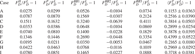
To better assess the flow information at the particle location, unladen cases corresponding to the nine examined cases are simulated, and the statistics of these unladen simulations are tabulated in table 4. These statistics (spatial and time averaged) are measured in a  $y$–
 $z$ plane sized
 $L^2$ centred at
 $(x_c - 0.5d_p,y_c,z_c)$, corresponding to the flow stagnation point in the particle-laden cases. A similar approach was used by Botto & Prosperetti (Reference Botto and Prosperetti2012), except that they measured the statistics from the
 $y$–
 $z$ plane corresponding to the particle centre. As shown in table 4, the turbulent incoming flows seen by the particle are indeed anisotropic. To assist the comparisons between the drag enhancements from the present study and those reported by Homann et al. (Reference Homann, Bec and Grauer2013), an overall r.m.s. velocity
 $\langle u'\rangle = \sqrt {(\langle u_x'\rangle ^2 + \langle u_y'\rangle ^2 + \langle u_z'\rangle ^2)/3}$ is defined for the present cases, and the turbulence intensity
 $I = \langle u'\rangle /U$ can be computed accordingly, as listed in table 4. It should be made clear that the purpose of conducting these unladen cases is not to obtain the instantaneous undisturbed fluid velocity to assess the reliability of the particle equations of motion, as intended in some previous studies (e.g. Bagchi & Balachandar Reference Bagchi and Balachandar2003; Burton & Eaton Reference Burton and Eaton2005; Zeng et al. Reference Zeng, Balachandar, Fischer and Najjar2008). In the present study, we are only interested in how the turbulence modifies the statistical average of the particle drag and how these modifications can be predicted from the statistics of the turbulent flows. The probability distribution functions (p.d.f.s) of
 $u_x'$,
 $u_y'$ and
 $u_z'$ in three selected cases out of the nine cases are shown in figure 4. It can be clearly seen that the distributions of the incoming flow velocities in all three directions are still close to Gaussian.
Information of the incoming flow.

The probability distribution functions (p.d.f.s) of the fluctuation velocity components of the incoming turbulent flows: (a) case C,  $I = 0.410$, (b) case E,
 $I = 0.265$, (c) case G,
 $I = 0.132$. The black solid line in each plot represents the Gaussian distribution.

The drag enhancement coefficient, defined as  $\langle F_D^T/F_D^L\rangle - 1$, where
 $\langle F_D^T\rangle$ and
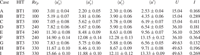
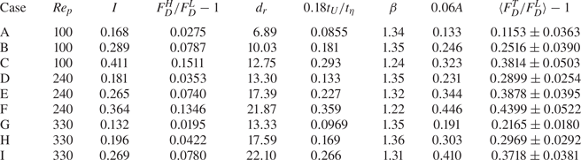
 $F_D^L$ are the time-averaged drag forces in turbulent and laminar flows, respectively, are plotted in figure 5, together with the results reported in the Homann et al. (Reference Homann, Bec and Grauer2013) study. To increase the accessibility of our data, they are also tabulated in table 5. It is evident that turbulence significantly enhances the drag forces on the particle in all cases. The empirical correlation suggested by Uhlherr & Sinclair (Reference Uhlherr and Sinclair1971) for drag coefficients of spherical particles in turbulent flows,
 \begin{equation} C_D^{US} = 0.133\left(1 + \frac{150}{Re_p}\right)^{1.565} + 4I,\quad 50< Re_p<700,\ 0.05< I<0.5, \end{equation}
is also shown in figure 5 by the dashed lines. Since this correlation does not apply to laminar flow, its corresponding results of  $\langle F_D^T/F_D^L\rangle - 1$ are computed as
 $C_D^{US}/C_{D}^{SN} - 1$, where
 $C_D^{SN}$ is the drag coefficient predicted by the Schiller & Naumann correlation. Uhlherr & Sinclair (Reference Uhlherr and Sinclair1971) predicted linear increases of drag enhancements with the turbulence intensity, which roughly agrees with the numerical data reported by Homann et al. (Reference Homann, Bec and Grauer2013) and this study. However, the quantitative values of the drag enhancement coefficients are significantly overestimated by the Uhlherr–Sinclair empirical correlation.
The drag enhancement coefficients under different turbulence intensities:  $\circ$, data from the present study;
 $*$, data from the Homann et al. (Reference Homann, Bec and Grauer2013) study; solid lines, nonlinear drag enhancements; dashed lines, the empirical correlation suggested by Uhlherr & Sinclair (Reference Uhlherr and Sinclair1971). Symbols and curves with the same colour have the same
 $Re_p$.

Comparison of nonlinear drag enhancement coefficients based on different models, and the actual drag enhancement coefficients from the simulations (last column).

The drag enhancement by turbulence, as analysed in the previous studies (e.g. Homann et al. Reference Homann, Bec and Grauer2013; Fornari et al. Reference Fornari, Picano, Sardina and Brandt2016b), is partially due to the nonlinear dependency of the particle drag on the flow velocity. Given that the incoming flow velocity is Gaussian distributed in each direction (confirmed in figure 4), Homann et al. (Reference Homann, Bec and Grauer2013) computed the averaged drag force as
 \begin{equation} F_{D}^{H} \equiv \int f^{iso}\left({\boldsymbol{u}}\right) F_{D}^{SN}\left({\boldsymbol{u}}\right) {\rm d}{\boldsymbol{u}},\quad {\boldsymbol{u}}=(U+u_x',u_y',u_z'), \end{equation}
where
 \begin{equation} F_{D}^{SN}\left({\boldsymbol{u}}\right) = 3{\rm \pi} d_p \mu \left[1 + 0.15\left(\frac{\vert{\boldsymbol{u}}\vert d_p}{\nu}\right)^{0.687}\right]\left({ \boldsymbol{u}}\boldsymbol{\cdot} {\boldsymbol{e}}_x\right) \end{equation}
is the drag force predicted by the Schiller & Naumann correlation and
 \begin{equation} f^{iso}({\boldsymbol{u}}) = \frac{1}{(\sqrt{2{\rm \pi}}\langle u'\rangle)^3 } \exp\left(-\frac{u_x'^2+u_y'^2+u_z'^2}{2 \langle u'\rangle^2}\right),\quad\langle u'\rangle = IU\end{equation}
is the p.d.f. of the instantaneous fluctuation velocity of the incoming flow assuming an isotropic distribution of TKE. The integral in (4.3a,b) can be numerically obtained, and the relative changes of  $\langle F_D^{H}/F_D^L\rangle - 1$ with the turbulence intensity are shown by the solid lines in figure 5. It is clear that the enhancements due to the nonlinear drag effect are below the actual drag enhancements and are
 $Re_p$ insensitive after
 $Re_p > 200$, which is different from the actual drag enhancement where
 $Re_p$ plays a much more important role. For the present cases where the incoming turbulent flows are anisotropic, the nonlinear drag
 $F_D^{P}$ can be computed by replacing
 $f^{iso}$ with a more general p.d.f.
 \begin{equation} f^{aniso}\left({\boldsymbol{u}}\right) = \frac{1}{(\sqrt{2{\rm \pi}})^3 \langle u_x'\rangle \langle u_y'\rangle \langle u_z'\rangle} \exp\left(-\frac{u_x'^2}{2 \langle u_x'\rangle^2}-\frac{u_y'^2}{2\langle u_y'\rangle^2}-\frac{u_z'^2}{2\langle u_z'\rangle^2}\right), \end{equation}
and with the information of  $\langle u_x'\rangle$,
 $\langle u_y'\rangle$ and
 $\langle u_z'\rangle$ in table 4. We also note that, in the earlier work of Bagchi & Balachandar (Reference Bagchi and Balachandar2003), two definitions of the particle drag force accounting for the nonlinear effect were proposed, and they are
 $$\begin{gather} F_{D}^{BB1} = \frac{1}{8}\rho_f {\rm \pi}d_p^2 \langle C_D^{SN}(Re_p)\vert {\boldsymbol{u}}\vert^2 \rangle,\quad Re_p = Re_p\left({\boldsymbol{u}}\right) = \frac{\vert {\boldsymbol{u}}\vert d_p}{\nu}, \end{gather}$$
 $$\begin{gather}F_{D}^{BB2} = \tfrac{1}{8}\rho_f {\rm \pi}d_p^2 C_D^{SN}\left(\langle Re_p\rangle\right) \vert\langle{\boldsymbol{u}}\rangle\vert^2 , \end{gather}$$
where
 \begin{align} \langle C_D^{SN}(Re_p)\vert {\boldsymbol{u}}\vert^2 \rangle = \int f^{aniso}\left({\boldsymbol{u}}\right)C_D^{SN}\left(Re_p\right)\vert {\boldsymbol{u}}\vert^2 \,{\rm d}{\boldsymbol{u}}, \quad \langle Re_{p}\rangle = \int f^{aniso}\left({\boldsymbol{u}}\right) Re_p\left({\boldsymbol{u}}\right) {\rm d}{\boldsymbol{u}}. \end{align}
Given the nonlinear dependency of the instantaneous drag force on the flow velocity, it would make more sense that the drag depends on the average of the velocity squared, i.e.  $\langle \vert {\boldsymbol {u}}\vert ^2\rangle$, rather than the square of the averaged velocity, i.e.
 $\vert \langle {\boldsymbol {u}}\rangle \vert ^2$ in (4.7b). With the Gaussian distribution of the fluctuation velocity, we shall also have
 $\langle \boldsymbol {u}\rangle = U\boldsymbol {e}_x$, which is constant. Based on this argument, a more reasonable definition for the nonlinear drag is formulated as
 \begin{equation}
F_{D}^{BB3} =
\tfrac{1}{8}\rho_f {\rm \pi}d_p^2 C_D^{SN}\left(\langle
Re_p\rangle\right)\langle\vert{\boldsymbol{u}}\vert^2\rangle,\quad\langle\vert{\boldsymbol{u}}\vert^2\rangle = \int f^{aniso}\left({\boldsymbol{u}}\right)
\vert{\boldsymbol{u}}\vert^2 \,{\rm d}{\boldsymbol{u}}.
\end{equation}
In table 5, these nonlinear drag enhancements are compared with the actual drag enhancements obtained from the numerical simulations. With the Homann et al. (Reference Homann, Bec and Grauer2013) definition of the nonlinear drag force, no matter whether the anisotropy in the incoming turbulent flows is considered, the nonlinear drag forces are significantly lower than their actual counterparts for all examined cases. With the Bagchi & Balachandar (Reference Bagchi and Balachandar2003) definition, the nonlinear drag forces are also considerably smaller than the actual drag forces, with only two exceptions in case B and case C. In particular, the original definition of the nonlinear drag in (4.7b) always shows drag reduction rather than drag enhancement, which could indicate this is an inappropriate estimation for the nonlinear drag. Compared with the Homann et al. (Reference Homann, Bec and Grauer2013) definition of nonlinear drag, the nonlinear drag of Bagchi & Balachandar (Reference Bagchi and Balachandar2003) is significantly higher. The difference is due to the different definitions of drag in the two works. In the Homann et al. (Reference Homann, Bec and Grauer2013) work, the drag was defined as the force component aligned with the mean flow direction, whereas in Bagchi & Balachandar (Reference Bagchi and Balachandar2003), it was the force aligned with the instantaneous relative velocity between the flow and the particle. Hence, the magnitudes of the latter are certainly higher. This detail partially explains the conflicting conclusions in the two works, i.e. Homann et al. (Reference Homann, Bec and Grauer2013) reported the inadequacy of using the nonlinear drag to explain the drag enhancement due to turbulence, while Bagchi & Balachandar (Reference Bagchi and Balachandar2003) claimed that the standard drag formula was already sufficient to predict the drag coefficient.
Based on the numerical results, this study adopts the Homann et al. (Reference Homann, Bec and Grauer2013) point and seeks mechanisms resulting in the differences between the nonlinear drag enhancements and the actual drag enhancements. It should be noted that, although the r.m.s. velocities of the turbulent flow are used in the calculation of  $\langle F_D^{H}\rangle$, the nonlinear drag enhancement is essentially a laminar effect, which also exists when the incoming flow is laminar but time dependent.
4.2. Additional mechanisms of drag enhancements
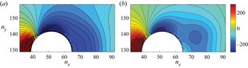
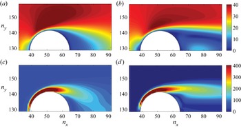
Homann et al. (Reference Homann, Bec and Grauer2013) attributed the gaps between the actual drag enhancements and the nonlinear drag enhancements to the interactions between the small turbulent eddies and the particle boundary layer. This deduction is reasonable, but the associated mechanisms have not been clarified. In order to better understand the mechanisms of how turbulence affects the particle drag, the flow fields around the particle is visualized. In figure 6, the pressure fields around the particle are visualized for case E and its corresponding laminar case with the same  $Re_p$. To ensure the two pressure fields can be compared at the same scale, we plot the deviation of the pressure from its instantaneous field mean, then average over 1000 time frames covering approximately 45 eddy turnover times, i.e.
 $\langle p(\boldsymbol {x}) \rangle - \langle P \rangle$. Although the wake structure is planar symmetric at this particle Reynolds number (
 $Re_p = 240$ in case E), the averaged pressure field still shows symmetry in the lower and top halves, so only half of the region is shown. To facilitate the following discussion, we locate
 $(x_c - 0.5d_p,y_c,z_c)$,
 $(x_c + 0.5d_p,y_c,z_c)$ and
 $(x_c,y_c+0.5d_p,z_c)$ as the front edge, trailing edge and the zenith, respectively. Compared with the laminar case, when the incoming flow is turbulent, the low-pressure region around the zenith is significantly extended, and the magnitudes of the pressure near the trailing edge are also reduced. These two changes certainly result in increased pressure drag. The pressure gradients between the high- and low-pressure regions are also enlarged by turbulence, as shown in the contours around the top-left corner. At the fixed particle Reynolds number
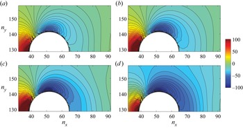
 $Re_p = 100$, the pressure contours from the laminar and turbulent flow cases with different intensities are compared in figure 7. It is clear that when the turbulence intensity increases, pressure gradients between the front edge and the zenith are further enhanced. As a result, the area of the low-pressure regions expands with the increase of the turbulence intensity, and the pressure in the low-pressure regions further decreases.
The pressure fields around the fixed particle in (a) case E and (b) the corresponding laminar flow.

The pressure contours around the particle in (a) the laminar flow, and turbulent flows with different intensities; (b) case A, (c) case B and (d) case C.

The strengthened low-pressure region in the turbulent cases also modifies the wake structures. Contours of the velocity magnitude and  $Q$-criterion (Jeong & Hussain Reference Jeong and Hussain1995) are compared in figure 8 for case E and its corresponding laminar case. More high-speed fluids outside the boundary layer are transported towards the symmetry axis in response to the strengthened low-pressure region around the trailing edge, which not only suppresses the circulation region but also results in faster restorations of the velocity deficiency, as reported in the previous studies (e.g. Bagchi & Balachandar Reference Bagchi and Balachandar2004; Homann et al. Reference Homann, Bec and Grauer2013).
Contours of the velocity magnitude and  $Q$-criterion in case E (a,c) and the corresponding laminar case (b,d). (a,b) Velocity magnitude, (c,d)
 $Q$-criterion.

As turbulence reduces the pressure behind the zenith, the region with adverse pressure gradients shrinks. This change postpones the separation of the boundary layer, as can be partially seen from figure 8. In the classic boundary layer theory, postponed separation usually results in drag reductions (Kundu, Cohen & Dowling Reference Kundu, Cohen and Dowling2015, Chap. 9). However, this is not the case in the present study. This exception is because, unlike the uniform incoming flow in the classic boundary layer theory, the incoming flows in the present cases are already turbulent. In the classic boundary layer theory, turbulent fluctuations mainly affect the pressure after the zenith by resisting the boundary layer separation, which leads to better pressure recovery to reduce the pressure drag (Kundu et al. Reference Kundu, Cohen and Dowling2015, Chap. 9). In the present study, however, a significant portion of the turbulence effect functions before the zenith, as shown by the amplified pressure gradients around the top-left corner in the turbulent cases, i.e. figures 6(a) and 7(b)–(d). In order to show this phenomenon more clearly, streamwise distributions of the planar fluid-phase-averaged pressure around the particle are computed in some selected laminar and turbulent cases. The averaging is processed over  $y$–
 $z$ planes with a size of
 $2.5d_p\times 2.5d_p$ that centre on the streamwise axis of the particle. As confirmed in figure 9, compared with the corresponding laminar case, the streamwise pressure gradient in the turbulent case is significantly larger, and most of the difference occurs before the zenith.
Additional pressure drop in the streamwise direction around the particle in a turbulent flow relative to that in a laminar flow. Here,  $P_0$ is the planar fluid-phase-averaged pressure at the front edge.

The amplified pressure gradients between the front edge and the zenith can be qualitatively understood by referring to the solution of the pressure field of the inviscid flow (Kundu et al. Reference Kundu, Cohen and Dowling2015, Chap. 4), where
 \begin{equation} p = p_{\infty} + \frac{1}{2}\rho U^2\left[\left(\frac{3a^3}{r^3} - \frac{3a^6}{4r^6}\right)\cos^2\theta - \left(\frac{a^3}{r^3} + \frac{a^6}{4r^6}\right) \right]. \end{equation}
The pressure gradient  $\partial p/\partial \theta$ yields
 \begin{equation} \frac{\partial p}{\partial \theta} ={-}\frac{1}{2}\rho U^2\left(\frac{3a^3}{r^3} - \frac{3a^6}{4r^6}\right)\sin\left(2\theta\right) . \end{equation}
The region between the front edge and the zenith is where  $\partial p/\partial \theta < 0$. The above solution does not apply rigorously for the present cases with viscous turbulent incoming flows. However, experimental measurements (Maxworthy Reference Maxworthy1969; Achenbach Reference Achenbach1972) found that the lowest pressure in a turbulent boundary layer around a sphere was still
 $\theta = 90$ degrees from the stagnation point and the pressure distribution was similar to the inviscid flow theory before the lowest pressure point. Despite the fact that these experimental measurements were conducted at much higher
 $Re_p$ than the present study, considering the similarity in their wake structures, it is reasonable to expect that the pressure gradient follows
 \begin{equation} \frac{\partial p}{\partial \theta} \propto \langle\vert {\boldsymbol{u}}\vert^2\rangle\sin\left(2\theta\right), \end{equation}
before the boundary layer separation. Equation (4.12) still predicts the lowest pressure at the zenith, which has been confirmed by the contour plots in figures 6 and 7. With the above assumption, it is clear that the more kinetic energy the flow has, the larger the pressure gradient expected. Compared with its laminar counterpart, a turbulent incoming flow has extra kinetic energy in the turbulent motions, i.e. TKE. Thus a greater pressure change is created, and also a greater resulting pressure drag. For the same reason, the pressure drop would further increase with the turbulence intensity. Since the large-scale motions mainly carry TKE in turbulent flows, this mechanism of pressure drag amplification is more associated with the large-scale eddies.
Different from large-scale eddies, the main effect of small turbulent eddies on the drag enhancement is to increase the velocity gradient in the particle boundary layer. This mechanism is the same one that increases the surface shear stress in the flat turbulent boundary layer. Since the particle has a finite size, the curvature of the particle might become unimportant for small scales in the turbulent flow. Unlike a laminar boundary layer that mainly transports momentum in the wall-normal direction via viscous diffusion, when turbulence is present, the small-scale velocity fluctuations in the wall-normal direction can directly bring high-speed fluids outside the boundary layer to the near-wall region and increase the velocity gradients there. As a result, the viscous drag is enhanced. With uniform incoming flows, this mechanism only occurs at very high Reynolds numbers after the transition from a laminar to a turbulent boundary layer occurs. In the present cases, the incoming flows are already turbulent, so the enhancement of the viscous drag by small turbulent eddies could happen at much lower Reynolds numbers. To confirm this mechanism, the streamwise velocity profiles along two lines,  ${\boldsymbol {e}}_1 = (0,1,0)$ and
 ${\boldsymbol {e}}_2 = (-1/\sqrt {2},1/\sqrt {2},0)$ across the particle centre are plotted in figure 10. The turbulent cases generally have larger streamwise velocity gradients than corresponding laminar cases, especially with smaller
 $Re_p$. When
 $Re_p$ increases, the relative increase of the streamwise velocity gradient due to turbulence reduces. Case E with
 $Re_p = 240$ has a similar turbulence intensity to that in case B with
 $Re_p = 100$, but its enhancements of streamwise velocity gradient are much less evident.
The distribution of the streamwise velocity along two selected lines across the particle centre: (a) a vertical line, (b) an inclined line.

4.3. Scaling of the drag enhancement
In the previous study of Homann et al. (Reference Homann, Bec and Grauer2013), it was reported that the drag enhancement coefficient  $F_D^T/F_D^L - 1$ scales well with
 $0.18t_U/t_\kappa$, where
 $t_U = d_p/U$ is the convective time, and
 $t_\kappa = (\nu /\varepsilon )^{0.5}$ is the Kolmogorov time. The data points from the present study are also plotted using this scaling in figure 11 together with the data reported in the Homann et al. (Reference Homann, Bec and Grauer2013) study. It is worth mentioning that the dissipation rates used to evaluate
 $t_\kappa = (\nu /\varepsilon )^{0.5}$ in the present study are estimated indirectly from
 $\langle \varepsilon \rangle = \langle u'\rangle ^{3}\langle \varepsilon _{HIT}\rangle /\langle u'_{HIT}\rangle ^{3}$, where
 $\langle u'_{HIT} \rangle$ and
 $\langle \varepsilon _{HIT} \rangle$ are measured from the sustained HIT in region A (table 1). This essentially assumes that the integral length scales
 $L$ are unchanged while the turbulent flows travel downstream, i.e.
 $L = \langle u'\rangle ^3/\langle \varepsilon \rangle$ is unchanged.
The drag enhancement coefficients under the Homann et al. (Reference Homann, Bec and Grauer2013) scaling.

As shown in figure 11, although the drag enhancement coefficients in the present study still qualitatively increase with  $t_U/t_\kappa$, their values are considerably higher than the predictions with the Homann et al. (Reference Homann, Bec and Grauer2013) scaling. These quantitative deviations are likely due to the difference in flow configurations. Specifically, as the turbulent flow loses isotropy while travelling downstream, the anisotropy of the turbulence could play an important role in the drag enhancement.
In order to see this point more clearly, a volume-averaged streamwise momentum balance analysis is conducted here. In recent years, such analyses have been widely employed to enhance the understanding of how particles modify the mean flow velocity and TKE in particle-laden turbulent channel and pipe flows (e.g. Picano, Breugem & Brandt Reference Picano, Breugem and Brandt2015; Yu et al. Reference Yu, Lin, Shao and Wang2017; Vreman & Kuerten Reference Vreman and Kuerten2018; Peng et al. Reference Peng, Ayala and Wang2019c). By volume averaging the streamwise momentum equation, the difference between the particle drag in turbulent and laminar flows is related to flow properties at the front and trailing edges of the particle as
 \begin{equation} \langle F_D^T - F_D^L\rangle \approx{-}\frac{1}{\Delta x}\left.\left( \frac{1}{\rho}P^T - \frac{1}{\rho}P^L + k_x^{T} - k_x^{L}\right)\right\rvert_{x_c-({1}/{2})d_p}^{x_c+({1}/{2})d_p}. \end{equation}
Detailed derivation of this equation is provided in Appendix A. Equation (4.13) shows that, in an ideal case, the particle drag enhancement due to turbulence is only related to two changes, the amplified pressure drops in the turbulent cases (as confirmed in figure 9) and the modification of the streamwise kinetic energy distribution. Compared with laminar boundary layers, turbulent boundary layers could provide more viscous dissipation to the kinetic energy, further increasing its drop in the streamwise direction. Since the modification of streamwise kinetic energy dominates the drag enhancement, in anisotropic turbulence, the influence of flow anisotropy should be considered when modelling the drag enhancement based on the fluid and particle parameters.
We start to seek an appropriate scaling by conducting a dimensional analysis. When the turbulent flow is homogeneous and isotropic, it is natural to think that the drag enhancement coefficient is a function of the turbulent r.m.s. velocity  $\langle u'\rangle$, dissipation rate
 $\langle \varepsilon \rangle$, viscosity
 $\nu$, the mean flow velocity
 $U$ and the particle diameter
 $d_p$, i.e.
 \begin{equation} \left\langle\frac{F_D^T}{F_D^L}\right\rangle - 1 = f\left(\langle u'\rangle, \langle\varepsilon\rangle, \nu, U, d_p\right). \end{equation}
The first three parameters define a HIT, while the last three define the particle Reynolds number. There are five dimensional parameters in this function and two basic units. Thus we can define three non-dimensional parameters, and they are
 \begin{equation} \left\langle\frac{F_D^T}{F_D^L}\right\rangle - 1 = f\left(\frac{\langle u'\rangle}{U}, \frac{d_p}{\eta}, \frac{U d_p}{\nu}\right) = f(I,d_r,Re_p), \end{equation}
where  $d_r = d_p/\eta$ is short-hand notation for the relative particle size. Note that, since the function is undetermined, we use the same
 $f$ in (4.14) and (4.15) for convenience. With some mathematical manipulation, the Homann et al. (Reference Homann, Bec and Grauer2013) scale
 $t_U/t_\kappa$ can be recast as
 $Re_p^{-1}d_r^2$, i.e.
 \begin{equation} \frac{t_U}{t_\eta} = \frac{d_p}{U}\left(\frac{\varepsilon}{\nu} \right)^{0.5}= \frac{\nu}{Ud_p}\frac{d_p^2}{\left(\nu^3/\varepsilon\right)^{0.5}} = Re_p^{{-}1}\left(\frac{d_p}{\eta}\right)^2 = Re_p^{{-}1}d_r^2, \end{equation}
which is a special form of (4.15). For a more general anisotropic turbulent flow, a single r.m.s. velocity  $\langle u'\rangle$ is no longer sufficient to describe the turbulence intensity, we therefore formulate
 \begin{equation} \left\langle\frac{F_D^T}{F_D^L}\right\rangle - 1 = f_{new}\left(\langle u_1'\rangle, \langle u_2'\rangle, \langle u_3'\rangle, \langle\varepsilon\rangle, \nu, U, d_p\right), \end{equation}
where  $\langle u_1'\rangle$,
 $\langle u_2'\rangle$ and
 $\langle u_3'\rangle$ are the component-wise r.m.s. velocities in three directions. Since the small scales in a turbulent flow are nearly isotropic, we keep
 $\langle \varepsilon \rangle$ rather than separating it into component-wise quantities. An alternative argument for this choice is that even the viscous dissipation is affected by anisotropic large-scale turbulent fluctuations as long as the time scales
 $\langle u_i\rangle ^2/\langle \varepsilon _i\rangle$ for different velocity components are comparable, thus there is still no need to divide
 $\langle \varepsilon \rangle$ into component-wise quantities. Compared with (4.15), the new function
 $f_{new}$ contains two additional non-dimensional parameters,
 $\beta _1 = \langle u_1'\rangle /\langle u_2'\rangle$ and
 $\beta _2 = \langle u_1'\rangle /\langle u_3'\rangle$ that measure the anisotropy of the turbulent flow. For convenience, we can always make
 $\langle u_1'\rangle$ the r.m.s. velocity in the streamwise direction that usually contains the largest TKE, i.e.
 $\beta _1 > 1$ and
 $\beta _2 > 1$. In the present study, the two cross-streamwise directions are symmetric, so only one parameter
 $\beta = (\beta _1\beta _2)^{0.5}$ is needed to measure the anisotropy. Equation (4.17) then becomes
 \begin{equation} \left\langle\frac{F_D^T}{F_D^L} \right\rangle- 1 = f_{new}(\beta, I,d_r,Re_p). \end{equation}
Taking  $\langle F_{D}^{T}/F_{D}^{L}\rangle - 1 \propto Re_p^{-1}d_r^2$ in Homann et al. (Reference Homann, Bec and Grauer2013) as the reference, it is reasonable to assume
 $f_{new}$ has power function dependencies on the four non-dimensional parameters, i.e.
 \begin{equation} \left\langle\frac{F_D^T}{F_D^L}\right\rangle - 1 = K\beta^{a}I^{b}d_r^{c}Re_p^{d}. \end{equation}
We can obtain the coefficients  $a$,
 $b$,
 $c$,
 $d$ and
 $K$ in two ways. The first is to assume the most general form in (4.19) and obtain the optimal values of the coefficients to fit the DNS data, which are tabulated for the nine simulated cases in table 6, via multi-dimensional linear regression. This method gives
 $a = 1.4$,
 $b = 0.5$,
 $c = 0.9$,
 $d = -0.1$ and
 $K = 0.06$. The comparison between the predictions of this scaling (
 $A = \beta ^{1.4}I^{0.5}d_r^{0.9}Re_p^{-0.1}$) and the numerical simulation results is shown in figure 12(a). The second method is to introduce the anisotropic correction on the basis of the Homann et al. (Reference Homann, Bec and Grauer2013) scale, i.e.
 $b = 0$,
 $c = 2$,
 $d = -1$ and
 $K = 0.18$. The optimal value for
 $a$ is obtained from linear regression as 1.8. The comparison between the model prediction of the second scaling (
 $B = \beta ^{1.8}d_r^{2}Re_p^{-1}$) and the numerical data is presented in figure 12(b). Good agreements between the prediction and the numerical results are observed in both plots. Scaling
 $A$ has a slightly better match to the numerical data than scaling
 $B$, but its formula is also slightly more complicated. Under both scalings, the anisotropy and the ratio between the particle size and the small turbulent eddies positively affect the relative drag enhancement, while the particle Reynolds number delivers negative impacts. For comparative purposes, the drag enhancement predicted by the nonlinear drag effect, Homann, Bec & Grauer Reference Homann, Bec and Grauer2013's scaling, and the present modified scalings are shown in table 6.
The drag enhancement coefficients under the revised scalings accounting for the anisotropy of the incoming turbulence flow.

Non-dimensional parameters in the modelling of drag enhancement. The fourth, sixth and eighth columns of the table represent the drag enhancements predicted by the nonlinear drag, the Homann et al. (Reference Homann, Bec and Grauer2013) scaling and the modified scaling. The DNS drag enhancements are shown in the last column.

4.4. The turbulent effect on the drag coefficient of particle arrays
Besides the single-particle cases discussed in the last section, cases with arrays of fixed particles in laminar and turbulent incoming flows are also investigated. The purpose is to understand how the lateral interactions among particles change the particle drag force. In order to reduce the computational cost, only three set-ups, cases B, D and E in table 4 are chosen. Case B and case E have similar turbulence intensities, while case D and case E have the same particle Reynolds number. Under each set-up, the number of particles varies to create particle arrays (see the sketch in figure 13) with different particle–particle relative gap distances, which are quantified by a non-dimensional parameter  $r_\rho = d_p/d$, where
 $d$ is the gap distance between the two nearest particles. The range of
 $r_\rho$ is chosen between
 $1/9$ and 1.5, corresponding to a layer of 1 to 36 uniformly distributed particles in region B. Particles in each simulation are placed at the same streamwise location as the corresponding single-particle case. Given a fixed number of 256 grid points in each cross-streamwise direction, further increasing
 $r_\rho$ may lead to the flow in the throat between two particles being unresolved. Therefore, to avoid sabotaging the reliability of the numerical results, very dense particle cases with
 $r_\rho > 1.5$ are not covered.
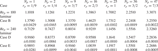
The drag coefficients of laminar and turbulent flows passing over arrays of particles.

The averaged drag coefficient in both the laminar and selected turbulent cases are shown in figure 13 and tabulated in table 7. With laminar incoming flows, the averaged drag force increases monotonically with  $r_\rho$, whereas with turbulent incoming flows, the drag coefficient decreases slightly at the beginning, then increases with
 $r_\rho$. The overall increased particle drag with
 $r_\rho$ also partially explains why the settling speed of multiple particles is lower compared with the sedimentation speed of individual particles, as reported in Fornari et al. (Reference Fornari, Picano and Brandt2016a). Besides the hindering effect and the nonlinear drag effect (Yin & Koch Reference Yin and Koch2007; Fornari et al. Reference Fornari, Picano and Brandt2016a), the lateral interactions between particles could also play an important role in the reduced settling speed for multiple particles.
The averaged drag coefficients for laminar and turbulent flow passing over particle arrays.

The increasing drag coefficient with  $r_\rho$ is not difficult to understand. As shown by the pressure contours in figure 14, when their distribution becomes denser, particles form contraction passages that force the flow to accelerate and lead to significantly amplified pressure drops between the particle front edge to the zenith location. In addition to this change, as particles approach each other, the low-pressure regions on the back of the particles merge and make the pressure recovery more difficult, which can be seen in figure 14. These two effects result in a significant increase in the pressure drag. Moreover, the flow acceleration in the contracted passages would create larger velocity gradients around particles and enhance the viscous drag. This latter mechanism is confirmed by the comparison of the streamwise velocity profiles along the two lines
 ${\boldsymbol {e}}_1 = (0,1,0)$ and
 ${\boldsymbol {e}}_{2} = (-1/\sqrt {2},1/\sqrt {2},0)$ across the particle centre, as shown in figure 15. When turbulence is present, the fluctuation motions of the turbulent eddies may partially counter these mechanisms and result in slight drag reduction. When
 $r_\rho$ further increases, these inverse effects eventually get overwhelmed, and enhancements of the drag coefficient are again observed. Nevertheless, more in-depth and decisive analyses are certainly needed to further confirm and reveal the subtle physics behind this inverse impact of turbulence on particle drag, which could be pursued in our future studies.
The comparison between the pressure contours of laminar and turbulent cases passing over arrays of particles with different particle–particle relative gap distances; (a,b)  $r_\rho = 1/9$, (c,d)
 $r_\rho = 1/4$, (e, f)
 $r_\rho = 1$; (a,c,e) laminar cases, (b,d, f) turbulent cases.

The distribution of the streamwise velocity along (a) a vertical line and (b) an inclined line across the particle centre.

The results of relative drag enhancement due to turbulence are shown in figure 16(a). In all examined cases, the enhancements of the drag coefficient due to turbulence decrease monotonically with  $r_\rho$ and eventually disappear around
 $r_\rho = 1.5$. This change essentially results from the fact that the drag enhancement due to the contracted passages dominates the contribution due to the turbulence, which is observed from the comparison of the pressure contours in figures 14(e)–14( f) and the comparison of the streamwise velocity distribution around the particle in figure 15. It is also observed that the changes in the drag enhancement coefficient with
 $r_\rho$ in different cases follow the same pattern.
The enhancement of the mean drag force as a function of  $r_\rho$: (a) relative drag enhancements compared with the laminar cases, (b) an empirical correlation for the relative drag enhancements.

Based on this observation, an empirical correlation to consider the effect of the particle–particle relative gap distance on the drag enhancement due to turbulence is proposed. Defining  $r_{\rho 0}$ as the
 $r_\rho$ with which the particle interaction can be fully ignored (cases with a single particle are roughly this type), the relative drag enhancement compared with its baseline value
 $\varTheta (r_{\rho 0}) = \langle F_D^T(r_{\rho 0})/F_D^L(r_{\rho 0})\rangle - 1$ approximately satisfies,
 \begin{equation} \varTheta(r_\rho) = \varTheta(r_{\rho0})\frac{-0.147(r_\rho - r_{\rho0})}{r_\rho - r_{\rho0} + 0.228}. \end{equation}
We emphasize that this correlation is generalized from our simulation results under relatively narrow ranges of parameter settings, i.e. the particle–particle relative gap distances  $1/9\leqslant r_\rho \leqslant 1.5$, particle Reynolds numbers
 $Re_p = 100$ and
 $240$ and turbulence intensities
 $0.18< I<0.3$. Applying the correlation for parameters beyond these ranges should proceed with caution.
5. Summary and conclusions
This work conducts direct numerical simulations of laminar and turbulent flows passing over fixed particles and particle arrays at moderate particle Reynolds numbers. Through systematically contrasting the results between the laminar and turbulent cases, two mechanisms of drag enhancement by turbulence are revealed, and more general scalings to quantify the drag enhancements are proposed to account for the influence of flow anisotropy. The main observations are summarized below.
(i) Compared with laminar flows, turbulent incoming flows amplify particle drag significantly. The nonlinear drag enhancement is insufficient to explain this amplification. This observation is consistent with those reported in the previous DNS study of Homann et al. (Reference Homann, Bec and Grauer2013) with a different flow configuration.
(ii) Aside from the nonlinear drag enhancement, two mechanisms are found responsible for the particle drag enhancement in turbulence. They are:
(a) The amplified streamwise pressure gradient due to the presence of TKE, which mainly occurs between the particle front edge and the zenith point, and is contributed by the large-scale fluctuations in the turbulent flows.
(b) The increased velocity gradient around the particle caused by the enhanced mixing of the low-speed fluid inside the boundary layer and the high-speed fluid outside, which is contributed by the small turbulent scales below the particle size.
(iii) The volume-averaged streamwise momentum analysis shows that the modifications of the streamwise kinetic energy make much more significant contributions to the drag enhancement than those in the other two directions. Based on this observation, the impact of flow anisotropy on drag enhancement must be considered. By dimensional analyses and fitting to the numerical data, the drag enhancement coefficient is found to scale with
 $A = \beta ^{1.4}I^{0.5}d_r^{0.9}Re_p^{-0.1}$, where $\beta$ is the parameter for flow anisotropy, $I$ is the turbulent intensity, $d_r$ is the relative particle size and $Re_p$ is the particle Reynolds number, or $B = \beta ^{1.8}d_r^{2}Re_p^{-1}$.
(iv) In laminar flows, the particle drag increases monotonically with decreasing particle–particle relative gap distance (quantified by
$r_\rho$), whereas in turbulent flows, the drag first decreases slightly and then increases with $r_\rho$. The impact of turbulence on the drag enhancement decreases monotonically with $r_\rho$ and disappears when $r_\rho = 1.5$ is reached.


A few unresolved puzzles are worth further investigation, particularly with multiple particles in turbulence. The minimum particle drag with  $r_\rho \approx 0.25$ in free-streaming turbulence certainly needs some further exploration. Whether the drag force enhancement correlation with
 $r_\rho$ is extendable to more general flow and particle parameters is also an open question. Furthermore, the present study only focuses on the turbulence effects on the averaged particle drag. How turbulence affects the level of fluctuations in the particle drag and how to model this aspect based on the flow and particle parameters have not been addressed. Answering those questions would better predict the settling speed of particles in turbulence, which will be pursued in our future studies.
Acknowledgements
Computing resources are provided by the National Supercomputing Center at Jinan and the Center for Computational Science and Engineering of the Southern University of Science and Technology.
Funding
This work has been supported by the National Natural Science Foundation of China (C.P., grant number 12102232, U2006221), (L.-P.W., grant number 91852205, 11961131006, U2241269); the Natural Science Foundation of Shandong Province, China (C.P., grant number 2022HWYQ-023, ZR2021QA010); the Taizhou-Shenzhen Innovation Center, Guangdong Provincial Key Laboratory of Turbulence Research and Applications (L.-P.W., 2019B21203001); Guangdong-Hong Kong-Macao Joint Laboratory for Data-Driven Fluid Mechanics and Engineering Applications (L.-P.W., grant number 2020B1212030001); and Shenzhen Science & Technology Program (L.-P.W., grant number KQTD20180411143441009). C.P. also acknowledges the financial support from Shandong University through the Qilu Young Scholar Program.
Declaration of interests
The authors report no conflict of interest.
Data availability statement
Data will be made available on request.
Appendix A. Derivation of the analytical drag enhancement
In the absence of the body force, the volume-averaged momentum equation of the fluid phase can be derived as (Crowe et al. Reference Crowe, Schwarzkopf, Sommerfeld and Tsuji2011)
 \begin{equation}
\frac{\partial}{\partial t}(\alpha \langle
u_{i}\rangle^f) + \frac{\partial}{\partial
x_{j}}(\alpha\langle u_{i}u_{j}\rangle^f) =
\frac{1}{\rho}\frac{\partial}{\partial
x_{j}}(\alpha\langle\sigma_{ij}\rangle^f)
+\frac{1}{\rho V}\int_{S_{I}}n_{j}\sigma_{ij}\,{\rm d}S,
\end{equation}
where  $\alpha$ is the volume fraction of the fluid phase in the control volume
 $V$,
 $\langle \cdots \rangle ^f$ indicates the phase averaging over the fluid phase,
 $\sigma _{ij}$ is the total stress tensor (pressure plus the viscous stress),
 $S_I$ is the flow–particle interface within the control volume
 $V$ and the last term in (A1) represents the force of the particle acting on the fluid phase. The last term in (A1) is the force acting on the fluid due to the presence of the particle (i.e.
 $n_j$ is the surface normal pointing into the particle) which is equal to
 $-F_i$, where
 $F_i$ is the force acting on the particle per unit mass of the averaging volume. At the steady state or statistically stationary state in the turbulent flow case, choosing the control volume
 $V$ as a very thin cuboid in the
 $y-z$ plane with thickness of
 $\Delta x$, the time-averaged momentum balance equation in the streamwise direction becomes
 \begin{equation}
\overline{F_x} ={-} \frac{\partial}{\partial
x_{j}}\left(\alpha\overline{\langle
u_{x}u_{j}\rangle^f}\right) +
\frac{1}{\rho}\frac{\partial}{\partial
x_{j}}\left(\alpha\overline{\langle\sigma_{xj}\rangle^f}\right),
\end{equation}
where the overbars  $\overline {\cdots }$ represent time averaging. When the flows are statistically homogeneous in the two cross-streamwise directions, e.g. in cases existing multiple free moving particles, the gradients in the two directions can be neglected, and the momentum balance equation in the streamwise direction becomes
 \begin{equation} \overline{F_x}
={-}\frac{1}{\rho}\frac{{\rm d} }{{\rm d}\kern0.06em x}\left(\alpha
\overline{\langle p\rangle^f}\right) - \frac{{\rm d}}{{\rm d}\kern0.06em x}\left(\alpha\overline{\langle u_{x}u_{x}\rangle^f}\right) + {2\nu}\frac{{\rm d}}{{\rm d}\kern0.06em x}\left(\alpha\overline{\left\langle \frac{\partial
u_x}{\partial x}\right\rangle^f}\right) .
\end{equation}
It should be emphasized that the statistics in the two cross-streamwise directions are deemed to be inhomogeneous with a single fixed particle. Thus (A3) does not apply rigorously. Extending the control volume  $V$ to the whole
 $y$–
 $z$ plane solves this conflict with the periodicity conditions in the two cross-streamwise directions. However, it would bring far-field information irrelevant to the particle drag change into the analysis. Therefore, the quantitative use of (A3) should proceed with caution.
With a fixed particle, the volume fraction of the fluid phase  $\alpha$ does not change with time, we would write
 $\overline {\langle \partial u_x/\partial x\rangle ^f} = {\rm d} \overline {\langle u_x\rangle ^f}/{{\rm d}\kern0.06em x}$. Applying the short-hand notation
 $\overline {\langle u_x\rangle ^f} = U_x$,
 $\overline {\langle p\rangle ^f} = P$, and
 $\overline {\langle u_x u_x\rangle ^f} = K_x$ to the laminar and turbulent cases, (A3) becomes
 $$\begin{gather} \overline{F_x^L}
={-}\frac{1}{\rho}\frac{{\rm d}}{{\rm d}\kern0.06em x}(\alpha
P^L) - \frac{{\rm d}}{{\rm d}\kern0.06em x}(\alpha
K_x^L) + {2\nu}\frac{{\rm d}}{{\rm d}\kern0.06em x}
\left(\alpha\frac{{\rm d} U_x^L}{{\rm d}\kern0.06em x}\right),
\end{gather}$$
 $$\begin{gather}\overline{F_x^T}
={-}\frac{1}{\rho}\frac{{\rm d}}{{\rm d}\kern0.06em x}(\alpha
P^T) - \frac{{\rm d}}{{\rm d}\kern0.06em x}(\alpha
K_x^T) + {2\nu}\frac{{\rm d}}{{\rm d}\kern0.06em x}
\left(\alpha\frac{{\rm d} U_x^T}{{\rm d}\kern0.06em x}\right),
\end{gather}$$
where the superscripts ‘ $T$’ and ‘
 $L$’ represent the laminar and turbulent flow cases. With the same control volume
 $V$ and particle size
 $d_p$ in the laminar and turbulent cases,
 $\alpha$ is identical. Thus, we use
 $\alpha$ instead of
 $\alpha ^L$ and
 $\alpha ^T$ in each case. The difference between the two equations is the drag enhancement contributed by the control volume
 $V$, i.e.
 \begin{align} \overline{F_x^T} -
\overline{F_x^L} ={-}\frac{1}{\rho}\frac{{\rm d}}{{\rm d}\kern0.06em x}[\alpha(P^T - P^L)] - \frac{{\rm
d}}{{\rm d}\kern0.06em x}[\alpha (K_x^T -
K_x^L)] + {2\nu}\frac{{\rm d}}{{\rm d}\kern0.06em x}\left[\alpha\left(\frac{{\rm d} U_x^T}{{\rm d}\kern0.06em x} -
\frac{{\rm d} U_x^L}{{\rm d}\kern0.06em x}\right)\right].
\end{align}
Again, when the flow is homogeneous in the two cross-streamwise directions or when  $V$ is extended to the whole domain, the continuity equation requires
 $\alpha U_x^T = \alpha U_x^L$, which essentially leads to
 $U_x^T = U_x^L$. As a result, (A5) further simplifies as
 \begin{equation} \overline{F_x^T} -
\overline{F_x^L} ={-}\frac{1}{\rho}\frac{{\rm d}}{{\rm d}\kern0.06em x}\left[\alpha(P^T - P^L)\right]- \frac{{\rm
d}}{{\rm d}\kern0.06em x}\left[\alpha(k_x^{T} - k_x^{L})\right], \end{equation}
where  $k_x = K_x - U_xU_x$ is the off-mean kinetic energy due to the inhomogeneous distribution of fluid velocity in the control volume, which can be non-zero even for the laminar case. Summing up the above equation from the control volume containing the front edge of the particle to the control volume containing the trailing edge of the particle, we have
 \begin{equation} \langle F_D^T -
F_D^L\rangle = \sum\left(\overline{F_x^T} -
\overline{F_x^L}\right) \approx{-}\frac{1}{\Delta
x}\left.\left( \frac{1}{\rho}P^T - \frac{1}{\rho}P^L +
k_x^{T} -
k_x^{L}\right)\right\vert_{x_c-({1}/{2})d_p}^{x_c+({1}/{2})d_p}.
\end{equation}
Note that, at the front and trailing edges of the particle,  $\alpha = 1$, thus they are omitted from the above equation.