1 Introduction
In many areas of science and engineering, a profound understanding of flow and heat transfer through spatially periodic solid structures is of utmost importance. Spatially periodic structures are found, for example, in the form of fin arrays or tube bundles within the flow passages of heat sinks and heat exchangers. Also in chemical reactors and fuel cells, the chemically reacting fluid typically passes through repetitive solid elements.
For a high number of solid structures, direct numerical simulation (DNS) of the flow and heat transfer is too demanding in terms of computational resources. Instead, simulation of the ‘macro-scale’ flow and temperature fields is more computationally efficient.
Models describing the macro-scale transport phenomena can be mathematically recovered from DNS models by a spatial filtering operation. In that case, the macro-scale quantities are defined in terms of a spatial average. The filter or averaging operator serves to remove the ‘micro-scale’ transport phenomena, which are the detailed phenomena occurring over a length scale smaller than the characteristic size of a single solid element. In the macro-scale models for single- and multiphase flow through porous media, the spatial filter is most often a simple volume average (Whitaker Reference Whitaker1999). The volume-averaging technique (VAT) is also commonly employed to describe the macro-scale flow and heat transfer in spatially periodic solid structures, such as tubes, fins or baffles.
As is the case for any macro-scale model derived through filtering of DNS transport equations, the volume-averaged flow and temperature equations contain so-called closure terms. These closure terms involve the effects of micro-scale transport phenomena around the fluid–solid interface and require additional modelling in order to solve the macro-scale transport equations. The closure terms arising in the filtered flow equations for an incompressible fluid are the interfacial force and momentum dispersion source. The three thermal closure terms which determine the macro-scale temperature of the fluid and solid, concern interfacial heat transfer, thermal tortuosity and thermal dispersion. Depending on the type of porous medium or solid structures under consideration, various approaches to determine the VAT closure terms have been proposed in the literature.
Whitaker (Reference Whitaker1996) showed theoretically that for many porous media, the closure terms in the volume-averaged incompressible flow equations can be approximated by means of a Darcy permeability tensor, a Forchheimer tensor and a momentum dispersion coefficient tensor, which are the solution of a periodic closure problem on a representative elementary volume (REV) of the porous medium. The thermal closure terms in the VAT equations for a porous medium can be determined on a REV of the medium by solving the general, yet complex, closure equations given by Quintard, Kaviany & Whitaker (Reference Quintard, Kaviany and Whitaker1997).
In case the fluid and solid phase of the porous medium are in local thermal equilibrium, their macro-scale temperature is the solution of a single macro-scale energy equation (Vafai & Tien Reference Vafai and Tien1981) containing just one closure term related to thermal dispersion. The numerical determination of the thermal dispersion term for the single macro-scale energy equation has been investigated e.g. by Hsu & Cheng (Reference Hsu and Cheng1990), Sahraoui & Kaviany (Reference Sahraoui and Kaviany1994), Kuwahara & Nakayama (Reference Kuwahara and Nakayama1999), Pedras & de Lemos (Reference Pedras and de Lemos2008). In the work of Nakayama, Kuwahara & Kodama (Reference Nakayama, Kuwahara and Kodama2006), thermal dispersion is modelled by a gradient-diffusion hypothesis in thermal equilibrium as well as non-equilibrium cases, for both laminar and turbulent flow.
For cases where the local thermal equilibrium condition does not hold, but the solid-to-fluid conductivity ratio within the porous medium is large, the closure model of DeGroot & Straatman (Reference DeGroot and Straatman2011) is valid. Numerical solutions of the former closure model have been correlated for a graphitic foam cell in the work of DeGroot & Straatman (Reference DeGroot and Straatman2012).
Whereas the flow through porous media which one encounters in aquifers or soils is fundamentally aperiodic in nature, laminar flow through a channel with periodic solid structures typically attains a periodic fully developed character (Patankar, Liu & Sparrow Reference Patankar, Liu and Sparrow1977) after a short entrance length. Therefore, for periodic solid structures it is essential to resolve the closure terms in the periodically developed flow and heat transfer regime.
Nakayama et al. (Reference Nakayama, Kuwahara, Umemoto and Hayashi2002), Nakayama, Kuwahara & Hayashi (Reference Nakayama, Kuwahara and Hayashi2004) represent the interfacial force in the periodically developed flow regime by means of a scalar permeability and Forchheimer coefficient. The authors follow the study of Kuwahara, Shirota & Nakayama (Reference Kuwahara, Shirota and Nakayama2001) and introduce an interfacial heat transfer coefficient to relate the heat transfer rate at the fluid–solid interface to the volume-averaged temperature difference between fluid and solid. They suggest that the former closure coefficients are spatially constant in case of a uniform macro-scale flow through an array of isothermal solid structures and can be governed by solving the periodically developed flow and temperature fields on a single unit of the array. Under these assumptions, their work presents numerically calculated coefficients for the VAT closure terms for an array of square cylinders with varying Reynolds number, macro-scale flow direction and cylinder spacing.
Also Alshare, Strykowski & Simon (Reference Alshare, Strykowski and Simon2010a ) investigated periodically developed flow and heat transfer on a unit cell of an array of square rods in order to correlate the VAT closure terms. Their study offers a correlation between the constant volume-averaged velocity and the constant unit cell pressure gradient in the developed regime for different flow angles, Reynolds numbers and rod configurations. While the previous studies (Kuwahara et al. Reference Kuwahara, Shirota and Nakayama2001; Nakayama et al. Reference Nakayama, Kuwahara, Umemoto and Hayashi2002, Reference Nakayama, Kuwahara and Hayashi2004) calculate the interfacial heat transfer coefficient in the developed regime for square rods at a constant temperature, Alshare et al. (Reference Alshare, Strykowski and Simon2010a ) correlate the heat transfer coefficient for a constant imposed temperature gradient over the unit cell. In addition, the authors provide dispersion coefficients for a range of flow angles to incorporate thermal dispersion in the macro-scale temperature equations. These dispersion coefficients are derived under the assumption of thermal equilibrium and extend the earlier work of e.g. Kuwahara, Nakayama & Koyama (Reference Kuwahara, Nakayama and Koyama1996), Kuwahara & Nakayama (Reference Kuwahara and Nakayama1999). Their closure correlations are applied and validated in a numerical model for the macro-scale velocity and temperature fields in a serpentine heat exchanger (Alshare, Strykowski & Simon Reference Alshare, Strykowski and Simon2010b ).
In the work of Horvat & Catton (Reference Horvat and Catton2003), Horvat & Mavko (Reference Horvat and Mavko2005), the VAT closure terms for a pin-fin array of a heat sink are modelled through a local drag and local heat transfer coefficient. In the first study (Horvat & Catton Reference Horvat and Catton2003), the local drag and local heat transfer coefficient are obtained from experimental correlations. In later work, Horvat & Mavko (Reference Horvat and Mavko2005) numerically calculate the local drag and heat transfer coefficient for a pin-fin element through a separate model assuming periodically developed flow and heat transfer conditions.
The determination of the VAT closure terms for periodic solid structures has continued to be a problem of interest, with applications to turbulent flow in heat sinks with circular and square pin fins (Catton Reference Catton2006), circular tube-fin heat exchangers (Zhou et al. Reference Zhou, Hansen, Geb and Catton2011) and heat sinks with elliptic scale-roughened surfaces (Zhou & Catton Reference Zhou and Catton2013).
However, in our previous work (Buckinx & Baelmans Reference Buckinx and Baelmans2015a ,Reference Buckinx and Baelmans b ), it has been shown that VAT is not always an appropriate filter technique for describing the macro-scale flow and heat transfer in periodic solid structures. First, the existing VAT closure models are all based on the assumption that some approximations (length scale constraints) for the temperature field are satisfied and that the spatial moments of the porous medium or solid structures are approximately zero. Although these assumptions seem reasonable for the transport regimes in a broad class of porous media, they introduce inaccuracies for solid structures in which the solid–fluid interface is exactly spatially periodic (Quintard & Whitaker Reference Quintard and Whitaker1994a ). Consequently, the VAT closure models do not yield exact closure of the macro-scale temperature equations in the periodically developed flow and heat transfer regime. Second, VAT complicates the determination of the closure terms, as it unavoidably leads to a spatially dependent interfacial force and macro-scale pressure gradient in the periodically developed flow regime (Buckinx & Baelmans Reference Buckinx and Baelmans2015b ). Also the heat transfer coefficient as well as other closure coefficients for the volume-averaged temperature equations are not spatially constant for the periodically developed heat transfer regime in isothermal solids (Buckinx & Baelmans Reference Buckinx and Baelmans2015a ).
To overcome the former shortcomings of VAT, we proposed a spatial filtering technique based on specific weighting functions, elaborating mainly on the work of Quintard & Whitaker (Reference Quintard and Whitaker1994b ), who gave a macro-scale description of creeping flow in ordered and disordered solid structures. Nevertheless, the theoretical foundations for the use of weighting functions for spatial averaging can be traced back to earlier studies on single- and multiphase flow through porous media. For example, the work of Marle (Reference Marle1965, Reference Marle1967), Hassanizadeh & Gray (Reference Hassanizadeh and Gray1979) as well as Baveye & Sposito (Reference Baveye and Sposito1984) should be mentioned.
This study applies the spatial filtering technique with weighting functions to give a mathematically profound macro-scale description of the periodically developed conjugate heat transfer regime, in which the temperature of the fluid and the temperature of the spatially periodic solid structures are coupled by a spatially periodic interfacial heat flux. We present a physically meaningful definition of the macro-scale temperature for this regime, which respects the physical analogies with developed channel flow under a constant heat flux. In addition, we derive a simple and exact closure model for this regime, that allows us to reconstruct both the full-scale temperature field and the macro-scale temperature field in full agreement with DNS predictions.
This paper starts with an overview of the definitions of the spatial averaging technique, building upon the framework of Quintard & Whitaker (Reference Quintard and Whitaker1994b ). In the next section, § 3, the spatially averaged temperature equations, describing the macro-scale temperature of the fluid and the solid structures, are briefly re-examined. In § 4, the characteristics of the periodically developed conjugate heat transfer regime are defined. The following section, § 5, discusses how the temperature gradient in the periodically developed conjugate heat transfer regime can be determined. The question how to choose the weighting function which defines a physically meaningful macro-scale temperature in the periodically developed conjugate heat transfer regime is answered in § 6. It is concluded that the weighting function of Quintard & Whitaker (Reference Quintard and Whitaker1994a ,Reference Quintard and Whitaker b ) or a double volume-average filter should be chosen. Subsequently, § 7 treats the exact form of the closure terms in the spatially averaged temperature equations for the double volume-average as well as for the single volume-average filter. It is shown that for the double volume-average filter, the interfacial heat transfer coefficient, tortuosity and thermal dispersion are spatially constant. Finally, in § 8, all theoretical derivations are illustrated for a two-dimensional flow through an array of solid squares.
2 Definitions of the spatial averaging theory
Every physical quantity
 $\unicode[STIX]{x1D719}$
, e.g. temperature
 $T$
, that is defined on a two- or three-dimensional continuum domain
 $\unicode[STIX]{x1D6FA}$
consisting of subregions of fluid (
 $\unicode[STIX]{x1D6FA}_{f}$
) and periodically arranged solid structures (
 $\unicode[STIX]{x1D6FA}_{s}$
) with a common interface boundary
 $\unicode[STIX]{x1D6E4}_{fs}$
, corresponds mathematically to a distribution (Gagnon Reference Gagnon1970; Schwartz Reference Schwartz1978):
 $$\begin{eqnarray}\unicode[STIX]{x1D719}(\boldsymbol{x},t)=\left\{\begin{array}{@{}ll@{}}\unicode[STIX]{x1D719}_{f}(\boldsymbol{x},t) & \text{in}~\unicode[STIX]{x1D6FA}_{f}\\ \unicode[STIX]{x1D719}_{s}(\boldsymbol{x},t) & \text{in}~\unicode[STIX]{x1D6FA}_{s}.\end{array}\right.\end{eqnarray}$$
Likewise, material properties which differ for the solid and fluid, for instance mass density
 $\unicode[STIX]{x1D70C}$
, specific heat capacity
 $c$
and heat conductivity
 $k$
, have a representation in the sense of a mathematical distribution as in (2.1). Flow quantities such as pressure
 $p$
, velocity field
 $\boldsymbol{u}$
, viscous stress field
 $\unicode[STIX]{x1D749}$
and viscosity
 $\unicode[STIX]{x1D707}$
are also represented in the form of (2.1), by defining them as zero in the solid region (
 $\unicode[STIX]{x1D719}_{s}=0$
).
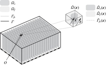
Three-dimensional continuum domain with periodically placed solid cylinders, averaging domain and interface boundary.

With every physical quantity we associate a filtered counterpart
 $\langle \unicode[STIX]{x1D719}\rangle _{m}$
, which is recovered after applying a filter or averaging operator
 $\langle \;\rangle _{m}$
on the corresponding distribution
 $\unicode[STIX]{x1D719}$
. The superficial spatial average,
 $\langle \unicode[STIX]{x1D719}\rangle _{m}$
, is defined by the linear convolution of
 $\unicode[STIX]{x1D719}$
with a normalized weighting function
 $m\in C^{\infty }$
having a compact support in
 $\unicode[STIX]{x1D6FA}$
and satisfying
 $m(\boldsymbol{x}-\boldsymbol{r})=0$
for
 $\boldsymbol{r}\notin \bar{\unicode[STIX]{x1D6FA}}(\boldsymbol{x})$
:
 $$\begin{eqnarray}\langle \unicode[STIX]{x1D719}\rangle _{m}|_{(\boldsymbol{x},t)}\triangleq \int _{\boldsymbol{r}\in \bar{\unicode[STIX]{x1D6FA}}(\boldsymbol{x})}m(\boldsymbol{x}-\boldsymbol{r})\unicode[STIX]{x1D719}(\boldsymbol{r},t)\,\text{d}\unicode[STIX]{x1D6FA}(\boldsymbol{r})\triangleq m\ast \unicode[STIX]{x1D719}.\end{eqnarray}$$
The filtered quantity
 $\langle \unicode[STIX]{x1D719}\rangle _{m}$
expresses a weighted average of the original distribution
 $\unicode[STIX]{x1D719}$
within a local averaging domain
 $\bar{\unicode[STIX]{x1D6FA}}$
of which the geometrical centroid
 $\boldsymbol{x}$
is a point of the domain
 $\unicode[STIX]{x1D6FA}$
(figure 1). Next to the superficial spatial average, we define the intrinsic spatial average of
 $\unicode[STIX]{x1D719}$
over the fluid and over the solid region:
 $$\begin{eqnarray}\langle \unicode[STIX]{x1D719}\rangle _{m}^{f}\triangleq \unicode[STIX]{x1D716}_{fm}^{-1}\langle \unicode[STIX]{x1D719}\unicode[STIX]{x1D6FE}_{f}\rangle _{m}\quad \text{and}\quad \langle \unicode[STIX]{x1D719}\rangle _{m}^{s}\triangleq \unicode[STIX]{x1D716}_{sm}^{-1}\langle \unicode[STIX]{x1D719}\unicode[STIX]{x1D6FE}_{s}\rangle _{m},\end{eqnarray}$$
where
 $\unicode[STIX]{x1D716}_{fm}\triangleq \langle \unicode[STIX]{x1D6FE}_{f}\rangle _{m}$
and
 $\unicode[STIX]{x1D716}_{sm}\triangleq \langle \unicode[STIX]{x1D6FE}_{s}\rangle _{m}$
are obtained by filtering the fluid and solid indicator
 $\unicode[STIX]{x1D6FE}_{f}$
and
 $\unicode[STIX]{x1D6FE}_{s}$
, which are defined as
 $\unicode[STIX]{x1D6FE}_{f}(\boldsymbol{x})=1$
if
 $\boldsymbol{x}\in \unicode[STIX]{x1D6FA}_{f}$
,
 $\unicode[STIX]{x1D6FE}_{f}(\boldsymbol{x})=0$
if
 $\boldsymbol{x}\in \unicode[STIX]{x1D6FA}_{s}$
and
 $\unicode[STIX]{x1D6FE}_{s}=1-\unicode[STIX]{x1D6FE}_{f}$
.
Each physical quantity also has an associated deviation part,
 $\tilde{\unicode[STIX]{x1D719}}$
, defined by the spatial decomposition
 $$\begin{eqnarray}\widetilde{\unicode[STIX]{x1D719}}\triangleq \unicode[STIX]{x1D719}-\langle \unicode[STIX]{x1D719}\rangle _{m}^{f}\unicode[STIX]{x1D6FE}_{f}-\langle \unicode[STIX]{x1D719}\rangle _{m}^{s}\unicode[STIX]{x1D6FE}_{s},\quad \text{so}~\unicode[STIX]{x1D719}=\langle \unicode[STIX]{x1D719}\rangle _{m}^{f}\unicode[STIX]{x1D6FE}_{f}+\langle \unicode[STIX]{x1D719}\rangle _{m}^{s}\unicode[STIX]{x1D6FE}_{s}+\widetilde{\unicode[STIX]{x1D719}}.\end{eqnarray}$$
The filtered distributions
 $\langle \unicode[STIX]{x1D719}\rangle _{m}$
,
 $\langle \unicode[STIX]{x1D719}\rangle _{m}^{f}$
and
 $\langle \unicode[STIX]{x1D719}\rangle _{m}^{s}$
correspond to macro-scale quantities provided that the filter operator meets two requirements. First, the filter operator should suppress the deviation part from the distribution:
 $\langle \tilde{\unicode[STIX]{x1D719}}\rangle _{m}\simeq 0$
, so that the filtered part remains approximately unaltered after repeated filtering:
 $\langle \langle \unicode[STIX]{x1D719}\rangle _{m}\rangle _{m}\simeq \langle \unicode[STIX]{x1D719}\rangle _{m}$
. Second, the filter should guarantee that the filtered parts
 $\langle \unicode[STIX]{x1D719}\rangle _{m}^{f}$
and
 $\langle \unicode[STIX]{x1D719}\rangle _{m}^{s}$
have significant gradients over a typical length scale
 $\mathscr{L}_{\unicode[STIX]{x1D719}}$
much larger than the spatial scale
 $\ell _{\unicode[STIX]{x1D719}}$
over which the full distribution
 $\unicode[STIX]{x1D719}$
, as well as its deviation part
 $\tilde{\unicode[STIX]{x1D719}}$
, undergo significant changes. Both requirements can be shown (Quintard & Whitaker Reference Quintard and Whitaker1994b
) to be equivalent to the requirement that the characteristic size
 $r_{m}$
of the filter window
 $\bar{\unicode[STIX]{x1D6FA}}$
satisfies the scale constraint
 $\ell _{\unicode[STIX]{x1D719}}\leqslant r_{m}\ll \mathscr{L}_{\unicode[STIX]{x1D719}}$
. The length scales are loosely defined by the order-of-magnitude estimates
 $\unicode[STIX]{x1D735}\langle T\rangle _{m}^{f}=O(\langle T\rangle _{m}^{f}/\mathscr{L}_{T})$
,
 $\unicode[STIX]{x1D735}\widetilde{T}=O(\widetilde{T}/\ell _{T})$
and
 $\langle \unicode[STIX]{x1D6FE}_{f}(\boldsymbol{r}-\boldsymbol{x})\rangle _{m}=O(\unicode[STIX]{x1D716}_{fm}r_{m})$
. When the filter operator ensures the former scale constraint, the deviation part of the distribution corresponds to a micro-scale quantity, so that the spatial decomposition according to (2.4) reflects a separation between the micro- and macro-scale levels.
In order to reformulate the physical laws for a physically conserved quantity within the theory of mathematical distributions, the time derivative in the usual sense and the gradient in the usual sense are introduced:
 $$\begin{eqnarray}\frac{\unicode[STIX]{x2202}^{\unicode[STIX]{x1D708}}\unicode[STIX]{x1D719}}{\unicode[STIX]{x2202}t}\triangleq \left\{\begin{array}{@{}ll@{}}\displaystyle \frac{\unicode[STIX]{x2202}\unicode[STIX]{x1D719}_{f}}{\unicode[STIX]{x2202}t} & \text{in}~\unicode[STIX]{x1D6FA}_{f}\\ \displaystyle \frac{\unicode[STIX]{x2202}\unicode[STIX]{x1D719}_{s}}{\unicode[STIX]{x2202}t} & \text{in}~\unicode[STIX]{x1D6FA}_{s}\end{array}\right.\quad \text{and}\quad \unicode[STIX]{x1D735}^{\unicode[STIX]{x1D708}}\unicode[STIX]{x1D719}\triangleq \left\{\begin{array}{@{}ll@{}}\unicode[STIX]{x1D735}\unicode[STIX]{x1D719}_{f} & \text{in}~\unicode[STIX]{x1D6FA}_{f}\\ \unicode[STIX]{x1D735}\unicode[STIX]{x1D719}_{s} & \text{in}~\unicode[STIX]{x1D6FA}_{s}.\end{array}\right.\end{eqnarray}$$
When the distribution
 $\unicode[STIX]{x1D719}$
is continuous at
 $\unicode[STIX]{x1D6E4}_{fs}$
,
 $\unicode[STIX]{x1D735}^{\unicode[STIX]{x1D708}}$
and
 $\unicode[STIX]{x2202}^{\unicode[STIX]{x1D708}}/\unicode[STIX]{x2202}t$
are equal to the ordinary gradient
 $\unicode[STIX]{x1D735}$
and ordinary time derivative
 $\unicode[STIX]{x2202}/\unicode[STIX]{x2202}t$
in
 $\unicode[STIX]{x1D6FA}$
.
The physical conservation laws for the filtered quantities often contain a so-called surface filter (Gagnon Reference Gagnon1970; Schwartz Reference Schwartz1978; Quintard & Whitaker Reference Quintard and Whitaker1994b ):
 $$\begin{eqnarray}\langle \boldsymbol{n}_{fs}(\unicode[STIX]{x1D719}_{f}-\unicode[STIX]{x1D719}_{s})\unicode[STIX]{x1D6FF}_{fs}\rangle _{m}|_{(\boldsymbol{x},t)}=\int _{\boldsymbol{r}\in \bar{\unicode[STIX]{x1D6E4}}_{fs}(\boldsymbol{x})}m(\boldsymbol{x}-\boldsymbol{r})\,\boldsymbol{n}_{fs}(\boldsymbol{r})(\unicode[STIX]{x1D719}_{f}(\boldsymbol{r},t)-\unicode[STIX]{x1D719}_{s}(\boldsymbol{r},t))\,\text{d}\unicode[STIX]{x1D6E4}(\boldsymbol{r}),\end{eqnarray}$$
which is an integral over the part of the fluid–solid interface within the averaging window that arises when the distribution is discontinuous at the fluid–solid interface, i.e. when
 $\unicode[STIX]{x1D719}_{f}(\boldsymbol{x},t)\neq \unicode[STIX]{x1D719}_{s}(\boldsymbol{x},t)$
for
 $\boldsymbol{x}\in \unicode[STIX]{x1D6E4}_{fs}$
. The surface filter relies on the concept of the Dirac distribution
 $\unicode[STIX]{x1D6FF}_{fs}$
associated with
 $\unicode[STIX]{x1D6E4}_{fs}$
and the unit normal vector
 $\boldsymbol{n}_{fs}$
at
 $\unicode[STIX]{x1D6E4}_{fs}$
, pointing from the
 $f$
-region towards the
 $s$
-region.
Furthermore, we introduce the geometrical tensors
 $\unicode[STIX]{x1D642}_{m}^{(n)}$
, which appear in the series expansion of the surface filter and which are related to the gradients of the spatial moments of the solid structures (Quintard & Whitaker Reference Quintard and Whitaker1994b
):
 $$\begin{eqnarray}\displaystyle \unicode[STIX]{x1D642}_{m}^{(n)}\triangleq \frac{1}{n!}\langle \boldsymbol{n}_{fs}(\boldsymbol{r}-\boldsymbol{x})^{\otimes n}\unicode[STIX]{x1D6FF}_{fs}\rangle _{m}=-\frac{1}{n!}\unicode[STIX]{x1D735}\langle \unicode[STIX]{x1D6FE}_{f}(\boldsymbol{r}-\boldsymbol{x})^{\otimes n}\rangle _{m}=\frac{1}{n!}\unicode[STIX]{x1D735}\langle \unicode[STIX]{x1D6FE}_{s}(\boldsymbol{r}-\boldsymbol{x})^{\otimes n}\rangle _{m}. & & \displaystyle\end{eqnarray}$$
Here,
 $\otimes n$
denotes the
 $n$
th tensor power of a tensor, which is the
 $n$
-fold tensor product of this tensor with itself. We remark that the repeated inner dot product between two tensors is denoted by repeated horizontal dots, e.g.
 $\boldsymbol{\cdot }\boldsymbol{\cdot }$
represents the double inner product.
In the remainder of this text, the context should make clear on which weighting function the filter operators
 $\langle \;\rangle _{m}$
,
 $\langle \;\rangle _{m}^{f}$
and
 $\langle \;\rangle _{m}^{s}$
are based. The weighting function
 $m_{V}$
for volume averaging is defined by
 $$\begin{eqnarray}m_{V}(\boldsymbol{x}-\boldsymbol{r})\triangleq \left\{\begin{array}{@{}ll@{}}\displaystyle \frac{1}{V} & \boldsymbol{r}\in \bar{\unicode[STIX]{x1D6FA}}(\boldsymbol{x})\\ 0 & \text{elsewhere}\end{array}\right.\quad \text{with}~V\triangleq \int _{\boldsymbol{r}\in \bar{\unicode[STIX]{x1D6FA}}(\boldsymbol{x})}\,\text{d}\unicode[STIX]{x1D6FA}(\boldsymbol{r}).\end{eqnarray}$$
In the case where
 $m=m_{V}$
is chosen, the index
 $m$
is dropped, so that the intrinsic volume-averaging operator for instance is represented by
 $\langle \;\rangle ^{f}$
and the volume-averaged fluid indicator or porosity is denoted by
 $\unicode[STIX]{x1D716}_{f}\triangleq \langle \unicode[STIX]{x1D6FE}_{f}\rangle$
.
Finally, we give the definition of the time average of a time-periodic distribution
 $\unicode[STIX]{x1D719}(\boldsymbol{x},t)=\unicode[STIX]{x1D719}(\boldsymbol{x},t+\unicode[STIX]{x1D70F})$
with period
 $\unicode[STIX]{x1D70F}$
:
 $$\begin{eqnarray}\overline{\unicode[STIX]{x1D719}}(\boldsymbol{x})\triangleq \frac{1}{\unicode[STIX]{x1D70F}}\int _{t-\unicode[STIX]{x1D70F}/2}^{t+\unicode[STIX]{x1D70F}/2}\unicode[STIX]{x1D719}(\boldsymbol{x},t^{\prime })\,\text{d}t^{\prime }.\end{eqnarray}$$
3 Spatially averaged temperature equations
When the temperature field and material properties are represented by generalized distributions as in (2.1), the principle of conservation of energy leads to the following equation for the macro-scale temperature
 $\langle T\rangle _{m}^{f}$
of the incompressible fluid (Buckinx & Baelmans Reference Buckinx and Baelmans2015a
):
 $$\begin{eqnarray}\displaystyle & & \displaystyle \unicode[STIX]{x1D70C}_{f}\unicode[STIX]{x1D716}_{fm}\frac{\unicode[STIX]{x2202}(c_{f}\langle T\rangle _{m}^{f})}{\unicode[STIX]{x2202}t}+\unicode[STIX]{x1D70C}_{f}\unicode[STIX]{x1D735}\boldsymbol{\cdot }(c_{f}\unicode[STIX]{x1D716}_{fm}\langle \boldsymbol{u}\rangle _{m}^{f}\langle T\rangle _{m}^{f})=\unicode[STIX]{x1D735}\boldsymbol{\cdot }k_{f}\unicode[STIX]{x1D735}(\unicode[STIX]{x1D716}_{fm}\langle T\rangle _{m}^{f})\nonumber\\ \displaystyle & & \displaystyle \qquad +\,\unicode[STIX]{x1D735}\boldsymbol{\cdot }k_{f}\langle \boldsymbol{n}_{fs}T_{f}\unicode[STIX]{x1D6FF}_{fs}\rangle _{m}+\langle \boldsymbol{n}_{fs}\boldsymbol{\cdot }(k_{f}\,\unicode[STIX]{x1D735}T_{f})\unicode[STIX]{x1D6FF}_{fs}\rangle _{m}-\unicode[STIX]{x1D70C}_{f}\unicode[STIX]{x1D735}\boldsymbol{\cdot }c_{f}\boldsymbol{D}+\unicode[STIX]{x1D716}_{fm}\langle \dot{q}\rangle _{m}^{f}+\unicode[STIX]{x1D716}_{fm}\langle \dot{q}_{visc}\rangle _{m}^{f},\nonumber\\ \displaystyle & & \displaystyle \qquad \text{where}~\boldsymbol{D}\triangleq \langle \boldsymbol{u}T\rangle _{m}-\unicode[STIX]{x1D716}_{fm}\langle \boldsymbol{u}\rangle _{m}^{f}\langle T\rangle _{m}^{f}.\end{eqnarray}$$
Here the symbols
 $\dot{q}$
and
 $\dot{q}_{visc}$
represent the volumetric heat source and viscous dissipation respectively. Energy conservation on the solid region implies the following equation for the macro-scale solid temperature
 $\langle T\rangle _{m}^{s}$
:
 $$\begin{eqnarray}\displaystyle \unicode[STIX]{x1D70C}_{s}\unicode[STIX]{x1D716}_{sm}\frac{\unicode[STIX]{x2202}(c_{s}\langle T\rangle _{m}^{s})}{\unicode[STIX]{x2202}t} & = & \displaystyle \unicode[STIX]{x1D735}\boldsymbol{\cdot }k_{s}\unicode[STIX]{x1D735}(\unicode[STIX]{x1D716}_{sm}\langle T\rangle _{m}^{s})-\unicode[STIX]{x1D735}\boldsymbol{\cdot }k_{s}\langle \boldsymbol{n}_{fs}T_{s}\unicode[STIX]{x1D6FF}_{fs}\rangle _{m}\nonumber\\ \displaystyle & & \displaystyle -\,\langle \boldsymbol{n}_{fs}\boldsymbol{\cdot }(k_{s}\unicode[STIX]{x1D735}T_{s})\unicode[STIX]{x1D6FF}_{fs}\rangle _{m}+\unicode[STIX]{x1D716}_{sm}\langle \dot{q}\rangle _{m}^{s}.\end{eqnarray}$$
The macro-scale temperature equations for the fluid and solid contain three thermal closure terms. The first closure term is the weighted thermal dispersion source,
 $$\begin{eqnarray}\boldsymbol{D}\triangleq \langle \boldsymbol{u}T\rangle _{m}-\unicode[STIX]{x1D716}_{fm}\langle \boldsymbol{u}\rangle _{m}^{f}\langle T\rangle _{m}^{f},\end{eqnarray}$$
which can be approximated as
 $\boldsymbol{D}\simeq \boldsymbol{D}_{approx}\triangleq \langle \widetilde{\boldsymbol{u}}\widetilde{T}\rangle _{m}$
if the filter window is small in comparison to the characteristic length scale over which the filtered temperature and filtered velocity change, i.e.
 $r_{m}\ll \mathscr{L}_{T}$
and
 $r_{m}\ll \mathscr{L}_{\boldsymbol{u}}$
, because
 $\langle \widetilde{\boldsymbol{u}}\rangle _{m}\simeq 0$
and
 $\langle \widetilde{T}\rangle _{m}\simeq 0$
in that case. The second closure term contains the heat flux at the fluid–solid interface,
 $q_{fs}=-\boldsymbol{n}_{fs}\boldsymbol{\cdot }k_{f}\,\unicode[STIX]{x1D735}T_{f}=-\boldsymbol{n}_{fs}\boldsymbol{\cdot }k_{s}\,\unicode[STIX]{x1D735}T_{s}$
, and defines the heat transfer coefficient
 $h_{fs}$
:
 $$\begin{eqnarray}\langle q_{fs}\unicode[STIX]{x1D6FF}_{fs}\rangle _{m}\triangleq h_{fs}(\langle T\rangle _{m}^{f}-\langle T\rangle _{m}^{s}).\end{eqnarray}$$
The interfacial heat transfer coefficient as defined here is consistent with the work of e.g. Kuwahara et al. (Reference Kuwahara, Shirota and Nakayama2001), Alshare et al. (Reference Alshare, Strykowski and Simon2010a ), Lopez Penha et al. (Reference Lopez Penha, Stolz, Kuerten, Nordlund, Kuczaj and Geurts2012) and correlates the mathematical form of the second closure term exactly for the periodically developed heat transfer regime in isothermal periodic solid structures (Buckinx & Baelmans Reference Buckinx and Baelmans2015a ). The last closure term is called the weighted thermal tortuosity and is given by
 $$\begin{eqnarray}\langle \boldsymbol{n}_{fs}T_{f}\unicode[STIX]{x1D6FF}_{fs}\rangle _{m}=\langle \boldsymbol{n}_{fs}T_{s}\unicode[STIX]{x1D6FF}_{fs}\rangle _{m}.\end{eqnarray}$$
It must be underlined that (3.1) and (3.2) have been called macro-scale equations, because it is assumed that both the weighting function
 $m$
as well as the size
 $r_{m}$
of the averaging window of the filter operator are carefully chosen to ensure separation of scales between the filtered temperature and filtered velocity and their deviation fields:
 $\ell _{T}\leqslant r_{m}\ll \mathscr{L}_{T}$
and
 $\ell _{\boldsymbol{u}}\leqslant r_{m}\ll \mathscr{L}_{\boldsymbol{u}}$
. If the filter operator would not yield a filtered temperature and filtered velocity field that vary over length scales
 $\mathscr{L}_{T}$
and
 $\mathscr{L}_{\boldsymbol{u}}$
larger than the characteristic scales
 $\ell _{T}$
and
 $\ell _{\boldsymbol{u}}$
over which the full temperature
 $T$
and full velocity field
 $\boldsymbol{u}$
change, there would be no computational benefit in numerically solving the filtered temperature equations, (3.1) and (3.2). The filtered temperature equations would need to be discretized on a mesh with the same spatial resolution as needed for accurately solving the full temperature equation through DNS of the Navier–Stokes equations.
The construction of an appropriate filter operator which respects the scale constraints is therefore of crucial importance. However, a practically useful filter operator should be more than just a mathematical tool to obtain separation of scales. It is also desired that the filter gives rise to a physically meaningful description, revealing the main features of the temperature and velocity fields. Lastly, the filter should lead to a simple and preferably exact model for the thermal closure terms in the macro-scale temperature equations. In this study, we investigate the form of the averaging operator which satisfies these three conditions for the periodically developed conjugate heat transfer regime. To this end, the next section first sets outs the characteristics of the periodically developed conjugate heat transfer regime in solid structures.
4 Periodically developed conjugate heat transfer
The periodically developed heat transfer regime in solid structures is characterized by the occurrence of a similarity between the profiles of the temperature distribution contained within different unit cells of the solid structures. In this context, a unit cell is defined as a local domain
 $$\begin{eqnarray}\unicode[STIX]{x1D6FA}_{unit}(\boldsymbol{x})\triangleq \left\{\boldsymbol{r}\,|\,\exists \,c_{j}\in \left(-\frac{1}{2},\frac{1}{2}\right)\Leftrightarrow \boldsymbol{r}=\boldsymbol{x}+\mathop{\sum }_{j=1}^{n_{j}}c_{j}\boldsymbol{l}^{(j)}\right\},\end{eqnarray}$$
spanned by the lattice vectors
 $\boldsymbol{l}^{(j)}$
, which themselves are defined through the periodicity of the fluid and solid indicators for any position
 $\boldsymbol{x}$
sufficiently far from the external boundary
 $\unicode[STIX]{x1D6E4}$
of the domain
 $\unicode[STIX]{x1D6FA}$
:
 $$\begin{eqnarray}\unicode[STIX]{x1D6FE}_{f}(\boldsymbol{x})=\unicode[STIX]{x1D6FE}_{f}(\boldsymbol{x}+\boldsymbol{l}^{(j)})=1-\unicode[STIX]{x1D6FE}_{s}(\boldsymbol{x})=1-\unicode[STIX]{x1D6FE}_{s}(\boldsymbol{x}+\boldsymbol{l}^{(j)})\quad \text{for}~j=1,\ldots ,n_{j}.\end{eqnarray}$$
Note that
 $n_{j}=2$
or
 $n_{j}=3$
, depending on whether it concerns a two- or three-dimensional unit cell.
The periodically developed heat transfer regime is the result of a flow field which varies in a periodic fashion from one unit cell to another at any time
 $t$
:
 $$\begin{eqnarray}\boldsymbol{u}(\boldsymbol{x},t)=\boldsymbol{u}(\boldsymbol{x}+\boldsymbol{l}^{(j)},t).\end{eqnarray}$$
In that case also the viscous dissipation
 $\dot{q}_{visc}\triangleq \unicode[STIX]{x1D749}\boldsymbol{\cdot }\boldsymbol{\cdot }\unicode[STIX]{x1D735}\boldsymbol{u}$
with
 $\unicode[STIX]{x1D749}=\unicode[STIX]{x1D707}_{f}(\unicode[STIX]{x1D735}\boldsymbol{u}+(\unicode[STIX]{x1D735}\boldsymbol{u})^{\intercal })$
is a spatially periodic term:
 $$\begin{eqnarray}\dot{q}_{visc}(\boldsymbol{x},t)=\dot{q}_{visc}(\boldsymbol{x}+\boldsymbol{l}^{(j)},t).\end{eqnarray}$$
We will assume that all time-dependent quantities in the periodically developed regime have a time-periodic behaviour, characterized by the same time period
 $\unicode[STIX]{x1D70F}$
, so that no initial conditions need to be specified for further analysis. Furthermore, for the periodically developed regime to occur, we consider it necessary that all material properties of the fluid and solid are constant.
In the periodically developed conjugate heat transfer regime, the similarity between the temperature profiles within different unit cells is attributed to the fact that the temperature distribution consists of a part that varies linearly in space with a constant gradient
 $\unicode[STIX]{x1D735}T$
, and a periodic part
 $T^{\star }$
that is similar for every unit cell (Patankar et al.
Reference Patankar, Liu and Sparrow1977; Lopez Penha et al.
Reference Lopez Penha, Stolz, Kuerten, Nordlund, Kuczaj and Geurts2012):
 $$\begin{eqnarray}T(\boldsymbol{x},t)=\unicode[STIX]{x1D735}T\boldsymbol{\cdot }(\boldsymbol{x}-\boldsymbol{x}_{0})+T^{\star }(\boldsymbol{x},t),\quad \text{with}~T^{\star }(\boldsymbol{x},t)=T^{\star }(\boldsymbol{x}+\boldsymbol{l}^{(j)},t).\end{eqnarray}$$
The term conjugate heat transfer regime is used because the former similarity occurs when the fluid and solid are subject to a spatially periodic volumetric heat source,
 $$\begin{eqnarray}\dot{q}(\boldsymbol{x},t)=\dot{q}(\boldsymbol{x}+\boldsymbol{l}^{(j)},t),\end{eqnarray}$$
and a spatially periodic interfacial heat flux,
 $$\begin{eqnarray}q_{fs}(\boldsymbol{x},t)=q_{fs}(\boldsymbol{x}+\boldsymbol{l}^{(j)},t)\quad \text{for}~\boldsymbol{x}\in \unicode[STIX]{x1D6E4}_{fs},\end{eqnarray}$$
which cause a coupling between the fluid temperature and solid temperature at the interface
 $\unicode[STIX]{x1D6E4}_{fs}$
.
In the periodically developed conjugate heat transfer regime, the periodic part
 $T^{\star }$
of the temperature field can be governed by solving the temperature equation for
 $T$
on a single unit cell, for an imposed temperature gradient
 $\unicode[STIX]{x1D735}T$
. The governing equation for
 $T^{\star }$
is given by
 $$\begin{eqnarray}\unicode[STIX]{x1D70C}\frac{\unicode[STIX]{x2202}^{\unicode[STIX]{x1D708}}(cT^{\star })}{\unicode[STIX]{x2202}t}+\unicode[STIX]{x1D70C}\unicode[STIX]{x1D735}\boldsymbol{\cdot }(\boldsymbol{u}cT^{\star })=\unicode[STIX]{x1D735}\boldsymbol{\cdot }(k\,\unicode[STIX]{x1D735}T^{\star })+\dot{q}_{visc}+\dot{q}-\unicode[STIX]{x1D70C}c\boldsymbol{u}\boldsymbol{\cdot }\unicode[STIX]{x1D735}T\quad \text{in}~\unicode[STIX]{x1D6FA}_{unit},\end{eqnarray}$$
with periodic boundary conditions
 $$\begin{eqnarray}T^{\star }(\boldsymbol{x},t)=T^{\star }(\boldsymbol{x}+\boldsymbol{l}^{(j)},t)\quad \text{where}~j=1,\ldots ,n_{j}.\end{eqnarray}$$
In order to solve (4.8) and (4.9) numerically, one should employ a discretization procedure which is able to cope with discontinuous transport coefficients (Lopez Penha et al.
Reference Lopez Penha, Stolz, Kuerten, Nordlund, Kuczaj and Geurts2012; Schroeder et al.
Reference Schroeder, Stomakhin, Howes and Teran2014), as the distributions
 $\unicode[STIX]{x1D70C}$
,
 $k$
and
 $c$
are discontinuous at the fluid–solid interface within the unit cell domain.
The need for such a discretization procedure can be circumvented by decomposing (4.8) into a set of two coupled equations which are to be solved separately on the fluid and solid region. The first of both equations determines the periodic temperature part
 $T_{f}^{\star }$
and is the restriction of (4.8) to the fluid region of the unit cell:
 $$\begin{eqnarray}\unicode[STIX]{x1D70C}_{f}\frac{\unicode[STIX]{x2202}(c_{f}T_{f}^{\star })}{\unicode[STIX]{x2202}t}+\unicode[STIX]{x1D70C}_{f}\unicode[STIX]{x1D735}\boldsymbol{\cdot }(\boldsymbol{u}_{f}c_{f}T_{f}^{\star })=\unicode[STIX]{x1D735}\boldsymbol{\cdot }(k_{f}\,\unicode[STIX]{x1D735}T_{f}^{\star })+\dot{q}_{visc}+\dot{q}_{f}-\unicode[STIX]{x1D70C}_{f}c_{f}\boldsymbol{u}_{f}\boldsymbol{\cdot }\unicode[STIX]{x1D735}T\quad \text{in}~\unicode[STIX]{x1D6FA}_{f}\cap \unicode[STIX]{x1D6FA}_{unit}.\end{eqnarray}$$
The second equation follows by restricting (4.8) to the solid region of the unit cell:
 $$\begin{eqnarray}\unicode[STIX]{x1D70C}_{s}\frac{\unicode[STIX]{x2202}(c_{s}T_{s}^{\star })}{\unicode[STIX]{x2202}t}=\unicode[STIX]{x1D735}\boldsymbol{\cdot }(k_{s}\,\unicode[STIX]{x1D735}T_{s}^{\star })+\dot{q}_{s}\quad \text{in}~\unicode[STIX]{x1D6FA}_{s}\cap \unicode[STIX]{x1D6FA}_{unit}.\end{eqnarray}$$
The former equations are coupled by the following boundary conditions at the interface:
 $$\begin{eqnarray}\displaystyle \left.\begin{array}{@{}c@{}}\displaystyle T_{f}^{\star }=T_{s}^{\star },\\ \displaystyle q_{fs}=-\boldsymbol{n}_{fs}\boldsymbol{\cdot }k_{f}(\unicode[STIX]{x1D735}T_{f}^{\star }+\unicode[STIX]{x1D735}T)=-\boldsymbol{n}_{fs}\boldsymbol{\cdot }k_{s}\,(\unicode[STIX]{x1D735}T_{s}^{\star }+\unicode[STIX]{x1D735}T)\quad \text{on}~\unicode[STIX]{x1D6E4}_{fs},\end{array}\right\} & & \displaystyle\end{eqnarray}$$
which impose the continuity of the temperature
 $T$
and the interfacial heat flux
 $q_{fs}$
at the interface. In addition, (4.10) and (4.11) are subject to the periodic boundary conditions
 $$\begin{eqnarray}\displaystyle T_{f}^{\star }(\boldsymbol{x},t)=T_{f}^{\star }(\boldsymbol{x}+\boldsymbol{l}^{(j)},t),\quad T_{s}^{\star }(\boldsymbol{x},t)=T_{s}^{\star }(\boldsymbol{x}+\boldsymbol{l}^{(j)},t)\quad \text{where}~j=1,\ldots ,n_{j}. & & \displaystyle\end{eqnarray}$$
The discretization of (4.10) and (4.11) is no longer hampered by the presence of discontinuous transport coefficients. Instead, a proper discretization of the coupling boundary conditions of (4.12) is required.
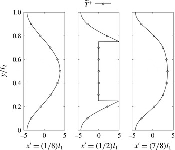
The governing equations for the periodically developed conjugate heat transfer regime, equations (4.8) and (4.9), or equivalently, equations (4.10)–(4.13), show that the periodic temperature similarity has the following functional dependence:
 $$\begin{eqnarray}T^{\star }=T^{\star }(\unicode[STIX]{x1D70C},c,k,\unicode[STIX]{x1D707}_{f},\unicode[STIX]{x1D6E4}_{fs}\cap \unicode[STIX]{x1D6FA}_{unit},\boldsymbol{u},\dot{q},\unicode[STIX]{x1D735}T,\boldsymbol{x},t).\end{eqnarray}$$
Hence, the periodic temperature part
 $T^{\star }$
in the periodically developed conjugate heat transfer regime is reconstructible from the knowledge of the material properties of fluid and solid, the geometry of the unit cell, the periodically developed velocity field, the periodic heat source and the temperature gradient over the unit cell. As the periodically developed flow field
 $\boldsymbol{u}$
is reconstructible from the spatially constant volume-averaged velocity
 $\langle \boldsymbol{u}\rangle$
over the unit cell domain (Buckinx & Baelmans Reference Buckinx and Baelmans2015b
),
 $\boldsymbol{u}$
can be replaced by
 $\langle \boldsymbol{u}\rangle$
in (4.14).
It must be remarked that the governing equations for the periodically developed conjugate heat transfer regime determine the periodic temperature part
 $T^{\star }$
only up to a constant. A unique solution for
 $T^{\star }$
is found by imposing for instance its time-and-volume-averaged value over the unit cell domain, so that
 $$\begin{eqnarray}\langle \overline{T^{\star }}\rangle =\text{const}.\end{eqnarray}$$
In matter of fact, the constant value of
 $\langle \overline{T^{\star }}\rangle$
is determined by the upstream temperature conditions just before the point where the heat transfer regime becomes periodically developed. Therefore, different values of
 $\langle \overline{T^{\star }}\rangle$
correspond to situations in which the fluid and solid pose a different average energy level over a unit cell after the onset of the periodically developed regime.
Finally, we add that (4.10), (4.12) and (4.13) also allow us to investigate the fluid temperature in the periodically developed regime for an imposed interfacial heat flux
 $q_{fs}$
. In the latter case, the solid temperature
 $T_{s}^{\star }$
is no longer resolved and (4.15) may be replaced by
 $\langle \overline{T^{\star }}\rangle ^{f}=\text{const.}$
, to find a unique solution for
 $T_{f}^{\star }$
. The functional dependence of the fluid temperature for an imposed interfacial heat flux looks like
 $$\begin{eqnarray}T_{f}^{\star }=T_{f}^{\star }(\unicode[STIX]{x1D70C}_{f},c_{f},k_{f},\unicode[STIX]{x1D707}_{f},\unicode[STIX]{x1D6E4}_{fs}\cap \unicode[STIX]{x1D6FA}_{unit},\langle \boldsymbol{u}\rangle ,q_{fs},\dot{q}_{f},\unicode[STIX]{x1D735}T,\boldsymbol{x},t).\end{eqnarray}$$
5 Temperature gradient for periodically developed conjugate heat transfer
The temperature gradient
 $\unicode[STIX]{x1D735}T$
in the periodically developed conjugate heat transfer regime is directly determined by the volumetric heat source and the viscous dissipation, through the relationship
 $$\begin{eqnarray}\frac{\unicode[STIX]{x2202}}{\unicode[STIX]{x2202}t}\langle \unicode[STIX]{x1D70C}cT^{\star }\rangle +\unicode[STIX]{x1D70C}_{f}c_{f}\langle \boldsymbol{u}\rangle \boldsymbol{\cdot }\unicode[STIX]{x1D735}T=\langle \dot{q}\rangle +\langle \dot{q}_{visc}\rangle ,\end{eqnarray}$$
which expresses an energy balance for the unit cell. The former energy balance is found after volume averaging (4.8) over the unit cell domain, taking
 $\bar{\unicode[STIX]{x1D6FA}}=\unicode[STIX]{x1D6FA}_{unit}$
for
 $m_{V}$
in (2.8). After averaging (5.1) over time and assuming time periodicity of the flow and temperature, we obtain
 $$\begin{eqnarray}\unicode[STIX]{x1D735}T=\frac{\langle \overline{\dot{q}}\rangle +\langle \overline{\dot{q}}_{visc}\rangle }{\unicode[STIX]{x1D70C}_{f}c_{f}\Vert \langle \overline{\boldsymbol{u}}\rangle \Vert }\boldsymbol{e}_{s}.\end{eqnarray}$$
Here, it was taken into account that by (5.1), the constant temperature gradient can have only a component along the direction of the time-and-volume-averaged velocity vector
 $\langle \overline{\boldsymbol{u}}\rangle \triangleq \Vert \langle \overline{\boldsymbol{u}}\rangle \Vert \boldsymbol{e}_{s}$
. For a steady flow, one can replace
 $\langle \overline{\boldsymbol{u}}\rangle =\langle \boldsymbol{u}\rangle$
in (5.2), which shows that the equality above is similar to the expression for the unit cell gradient derived by Lopez Penha et al. (Reference Lopez Penha, Stolz, Kuerten, Nordlund, Kuczaj and Geurts2012) in search of a steady solution of the temperature equation (4.8). In this way, equation (5.2) generalizes their result towards time-periodic developed flow fields for which the volume-averaged velocity
 $\langle \boldsymbol{u}\rangle$
changes over time, as considered in Ghaddar (Reference Ghaddar1995), Buckinx & Baelmans (Reference Buckinx and Baelmans2015b
).
It is interesting to note that the temperature gradient is also determined by the interfacial heat flux
 $q_{fs}$
via the energy balance for the fluid within the unit cell,
 $$\begin{eqnarray}\unicode[STIX]{x1D70C}_{f}c_{f}\unicode[STIX]{x1D716}_{f}\frac{\unicode[STIX]{x2202}\langle T^{\star }\rangle ^{f}}{\unicode[STIX]{x2202}t}+\unicode[STIX]{x1D70C}_{f}c_{f}\langle \boldsymbol{u}\rangle \boldsymbol{\cdot }\unicode[STIX]{x1D735}T=\langle q_{fs}\unicode[STIX]{x1D6FF}_{fs}\rangle +\unicode[STIX]{x1D716}_{f}\langle \dot{q}\rangle ^{f}+\unicode[STIX]{x1D716}_{f}\langle \dot{q}_{visc}\rangle ^{f}.\end{eqnarray}$$
This energy balance for the fluid within the unit cell domain follows from multiplying each term of (4.8) with
 $\unicode[STIX]{x1D6FE}_{f}$
, before averaging each term over the unit cell domain. After time averaging (5.3), we thus also have
 $$\begin{eqnarray}\unicode[STIX]{x1D735}T=\frac{\langle \overline{q}_{fs}\unicode[STIX]{x1D6FF}_{fs}\rangle +\unicode[STIX]{x1D716}_{f}\langle \overline{\dot{q}}\rangle ^{f}+\unicode[STIX]{x1D716}_{f}\langle \overline{\dot{q}}_{visc}\rangle ^{f}}{\unicode[STIX]{x1D70C}_{f}c_{f}\Vert \langle \overline{\boldsymbol{u}}\rangle \Vert }\boldsymbol{e}_{s}.\end{eqnarray}$$
The time-averaged energy balances of (5.2) and (5.4) allow for the calculation of the unit cell temperature gradient from all the parameters that determine
 $T^{\star }$
. Consequently,
 $\unicode[STIX]{x1D735}T$
can be left out the functional relationship (4.14) for the periodic temperature part. Likewise, when the solid temperature is not resolved, but just the functional dependence of the fluid temperature
 $T_{f}^{\star }$
for an imposed heat flux is of interest, equation (5.4) relates
 $\unicode[STIX]{x1D735}T$
to
 $q_{fs}$
, so that
 $\unicode[STIX]{x1D735}T$
can be left out the functional relationship (4.16) for
 $T_{f}^{\star }$
. This leads to the conclusion that the full-scale temperature field
 $T$
and all the closure terms in the periodically developed conjugate heat transfer regime are entirely determined by the parameter set
 $\{\unicode[STIX]{x1D70C},c,k,\unicode[STIX]{x1D707}_{f},\unicode[STIX]{x1D6E4}_{fs}\cap \unicode[STIX]{x1D6FA}_{unit},\langle \boldsymbol{u}\rangle ,\dot{q},\boldsymbol{x},t\}$
, or
 $\{\unicode[STIX]{x1D70C}_{f},c_{f},k_{f},\unicode[STIX]{x1D707}_{f},\unicode[STIX]{x1D6E4}_{fs}\cap \unicode[STIX]{x1D6FA}_{unit},\langle \boldsymbol{u}\rangle ,\dot{q},q_{fs},\boldsymbol{x},t\}$
if the heat flux is known.
In this section, the relationship between the unit cell temperature gradient and the heat sources has been found via the simple volume-averaging technique. The results (5.2) and (5.4) could also have been derived using a more general filter of the form
 $m=m_{G}\ast m_{V}$
, where
 $m_{G}$
is an arbitrary function, as long as
 $\bar{\unicode[STIX]{x1D6FA}}=\unicode[STIX]{x1D6FA}_{unit}$
for
 $m_{V}$
. In the next section, we will show that the appropriate weighting function for the periodically developed conjugate heat transfer regime indeed has the form
 $m=m_{G}\ast m_{V}$
, so that the relations (5.2) and (5.4) remain consistent with the following analysis.
6 Choice of weighting function for the macro-scale temperature
The appropriate filter for the periodically developed conjugate heat transfer regime should at least define a physically meaningful macro-scale temperature for this regime. To construct the appropriate filter, we first explore for which type of filter, the filtered temperature
 $\langle T\rangle _{m}$
represents an averaged impression of the original temperature
 $T$
which remains unaltered after successive averaging. In other words, we first require the filter to respect that
 $\langle \langle T\rangle _{m}\rangle _{m}\simeq \langle T\rangle _{m}$
in order to have a meaningful averaged temperature. In general, the requirement
 $\langle \langle T\rangle _{m}\rangle _{m}\simeq \langle T\rangle _{m}$
is fulfilled when the filter suppresses the gradients and other higher-order derivatives of the filtered temperature distribution, as can be seen from the Taylor series for the double filtered temperature,
 $$\begin{eqnarray}\langle \langle T\rangle _{m}\rangle _{m}|_{(\boldsymbol{x},t)}=\langle T\rangle _{m}|_{(\boldsymbol{x},t)}+\mathop{\sum }_{n=1}^{\infty }\frac{1}{n!}\langle (\boldsymbol{r}-\boldsymbol{x})^{\otimes n}\rangle _{m}|_{\boldsymbol{x}}\underbrace{\boldsymbol{\cdot }\boldsymbol{\cdot }}_{n\text{-times}}\unicode[STIX]{x1D735}^{\otimes n}\langle T\rangle _{m}|_{(\boldsymbol{x},t)}.\end{eqnarray}$$
After substitution of (4.5), the right-hand side of the former Taylor series becomes
 $$\begin{eqnarray}\langle T\rangle _{m}|_{(\boldsymbol{x},t)}+\langle (\boldsymbol{r}-\boldsymbol{x})\rangle _{m}|_{\boldsymbol{x}}\boldsymbol{\cdot }\unicode[STIX]{x1D735}T+\mathop{\sum }_{n=1}^{\infty }\frac{1}{n!}\langle (\boldsymbol{r}-\boldsymbol{x})^{\otimes n}\rangle _{m}|_{\boldsymbol{x}}\underbrace{\boldsymbol{\cdot }\boldsymbol{\cdot }}_{n\text{-times}}\unicode[STIX]{x1D735}^{\otimes n}\langle T^{\star }\rangle _{m}|_{(\boldsymbol{x},t)}.\end{eqnarray}$$
This result shows that the appropriate filter for the periodically developed conjugate heat transfer regime should be based on a weighting function of the form
 $m=m_{G}\ast m_{V}$
, where the filter window of
 $m_{V}$
coincides with the unit cell domain and
 $m_{G}$
is an arbitrary weighting function, because then
 $\langle \langle T\rangle _{m}\rangle _{m}=\langle T\rangle _{m}$
holds exactly. Indeed, for any filter based on
 $m=m_{G}\ast m_{V}$
with
 $\bar{\unicode[STIX]{x1D6FA}}=\unicode[STIX]{x1D6FA}_{unit}$
for
 $m_{V}$
in (2.8), it holds that
 $\langle (\boldsymbol{r}-\boldsymbol{x})\rangle _{m}|_{\boldsymbol{x}}=0$
, because
 $\boldsymbol{x}$
corresponds to the geometrical centroid of the averaging window. Furthermore, this form of the filter invokes that the last term in (6.2) vanishes as
 $\langle T^{\star }\rangle _{m}$
is constant, because
 $$\begin{eqnarray}\unicode[STIX]{x1D719}(\boldsymbol{x})=\unicode[STIX]{x1D719}(\boldsymbol{x}+\boldsymbol{l}^{(j)})\quad \Rightarrow \quad \left\{\begin{array}{@{}l@{}}\langle \unicode[STIX]{x1D719}\rangle _{m}=\langle \langle \unicode[STIX]{x1D719}\rangle \rangle _{m_{G}}=\langle \unicode[STIX]{x1D719}\rangle =\text{const}.\\ \langle \widetilde{\unicode[STIX]{x1D719}}\rangle _{m}=\langle \widetilde{\unicode[STIX]{x1D719}}\rangle =0,\end{array}\right.\end{eqnarray}$$
for any spatially periodic distribution
 $\unicode[STIX]{x1D719}$
in that case.
With the appropriate filter form
 $m=m_{G}\ast m_{V}$
, the superficially averaged temperature in the periodically developed conjugate heat transfer regime,
 $$\begin{eqnarray}\langle T\rangle _{m}=\unicode[STIX]{x1D735}T\boldsymbol{\cdot }(\langle (\boldsymbol{r}-\boldsymbol{x})\rangle _{m}+(\boldsymbol{x}-\boldsymbol{x}_{0}))+\langle T^{\star }\rangle _{m},\end{eqnarray}$$
varies linearly over space as
 $\langle (\boldsymbol{r}-\boldsymbol{x})\rangle _{m}=0$
and the filtered temperature gradient,
 $$\begin{eqnarray}\displaystyle \unicode[STIX]{x1D735}\langle T\rangle _{m}=(\unicode[STIX]{x1D735}\langle (\boldsymbol{r}-\boldsymbol{x})\rangle _{m}+\unicode[STIX]{x1D644})\boldsymbol{\cdot }\unicode[STIX]{x1D735}T+\unicode[STIX]{x1D735}\langle T^{\star }\rangle _{m}=\unicode[STIX]{x1D735}T+\unicode[STIX]{x1D735}\langle T^{\star }\rangle _{m}, & & \displaystyle\end{eqnarray}$$
becomes equal to the constant temperature gradient:
 $\unicode[STIX]{x1D735}\langle T\rangle _{m}=\unicode[STIX]{x1D735}T$
.
In order to have also a meaningful intrinsically averaged temperature of the fluid and solid, we need to ensure that the filter in addition respects that
 $\langle \langle T\rangle _{m}^{f}\rangle _{m}^{f}\simeq \langle T\rangle _{m}^{f}$
and
 $\langle \langle T\rangle _{m}^{s}\rangle _{m}^{s}\simeq \langle T\rangle _{m}^{s}$
. Because the intrinsically averaged fluid temperature in the periodically developed conjugate heat transfer regime is given by
 $$\begin{eqnarray}\langle T\rangle _{m}^{f}=\unicode[STIX]{x1D735}T\boldsymbol{\cdot }(\langle \unicode[STIX]{x1D6FE}_{f}(\boldsymbol{r}-\boldsymbol{x})\rangle _{m}^{f}+(\boldsymbol{x}-\boldsymbol{x}_{0}))+\langle T^{\star }\rangle _{m}^{f}\end{eqnarray}$$
and the intrinsically averaged solid temperature is given by
 $$\begin{eqnarray}\langle T\rangle _{m}^{s}=\unicode[STIX]{x1D735}T\boldsymbol{\cdot }(\langle \unicode[STIX]{x1D6FE}_{s}(\boldsymbol{r}-\boldsymbol{x})\rangle _{m}^{s}+(\boldsymbol{x}-\boldsymbol{x}_{0}))+\langle T^{\star }\rangle _{m}^{s},\end{eqnarray}$$
the requirements
 $\langle \langle T\rangle _{m}^{f}\rangle _{m}^{f}=\langle T\rangle _{m}^{f}$
and
 $\langle \langle T\rangle _{m}^{s}\rangle _{m}^{s}=\langle T\rangle _{m}^{s}$
are satisfied exactly if the filter operator suppresses the first-order spatial moments of the solid structures, which means that
 $\langle \unicode[STIX]{x1D6FE}_{f}(\boldsymbol{r}-\boldsymbol{x})\rangle _{m}^{f}=\langle \unicode[STIX]{x1D6FE}_{s}(\boldsymbol{r}-\boldsymbol{x})\rangle _{m}^{s}=0$
. This filter property is achieved by choosing
 $m_{G}$
of the form
 $m_{G}=m_{C}\ast m_{V}$
, where
 $m_{C}$
is yet to be determined, because with the overall weighting function
 $m=m_{C}\ast m_{V}\ast m_{V}$
, the filter ensures that all odd spatial moments of the solid structures vanish (Quintard & Whitaker Reference Quintard and Whitaker1994b
):
 $$\begin{eqnarray}\langle \unicode[STIX]{x1D6FE}_{f}(\boldsymbol{r}-\boldsymbol{x})^{\otimes n}\rangle _{m}=0\quad \text{and}\quad \langle \unicode[STIX]{x1D6FE}_{s}(\boldsymbol{r}-\boldsymbol{x})^{\otimes n}\rangle _{m}=0\quad \text{if}~n~\text{is odd}.\end{eqnarray}$$
Due to the property that
 $\langle \langle T\rangle _{m}^{f}\rangle _{m}^{f}=\langle T\rangle _{m}^{f}$
and
 $\langle \langle T\rangle _{m}^{s}\rangle _{m}^{s}=\langle T\rangle _{m}^{s}$
, the appropriate filter guarantees that the temperature changes occurring over the smallest length scales, which are contained within the temperature deviation part
 $\widetilde{T}$
, are filtered away:
 $\langle \widetilde{T}\rangle _{m}=0$
. The fact that
 $\langle \widetilde{T}\rangle _{m}=0$
for the weighting function
 $m=m_{C}\ast m_{V}\ast m_{V}$
is easily verified from the expression for the temperature deviation in the periodically developed conjugate heat transfer regime,
 $$\begin{eqnarray}\widetilde{T}=T^{\star }-\langle T^{\star }\rangle _{m}^{f}\unicode[STIX]{x1D6FE}_{f}-\langle T^{\star }\rangle _{m}^{s}\unicode[STIX]{x1D6FE}_{s}-\unicode[STIX]{x1D735}T\boldsymbol{\cdot }(\langle \unicode[STIX]{x1D6FE}_{f}(\boldsymbol{r}-\boldsymbol{x})\rangle _{m}^{f}\unicode[STIX]{x1D6FE}_{f}+\langle \unicode[STIX]{x1D6FE}_{s}(\boldsymbol{r}-\boldsymbol{x})\rangle _{m}^{s}\unicode[STIX]{x1D6FE}_{s}),\end{eqnarray}$$
which proves that
 $\langle \widetilde{T}\rangle _{m}=0$
is a direct consequence of (6.8).
Another consequence of (6.8) is that the intrinsically averaged temperature of the fluid and solid have the same constant gradient
 $\unicode[STIX]{x1D735}\langle T\rangle _{m}^{f}=\unicode[STIX]{x1D735}\langle T\rangle _{m}^{s}=\unicode[STIX]{x1D735}T$
as the superficially averaged temperature. Thus, the appropriate filter with
 $m=m_{C}\ast m_{V}\ast m_{V}$
leads to a linearly varying filtered temperature of the fluid and solid and a spatially constant filtered interfacial heat flux
 $\langle q_{fs}\rangle _{m}=\langle q_{fs}\rangle$
in the periodically developed conjugate heat transfer regime. As this resembles an analogy with developed channel flow in which the fluid bulk temperature varies linearly in the main flow direction when the heat flux from the solid wall is constant, we argue that the weighting function
 $m=m_{C}\ast m_{V}\ast m_{V}$
is also needed to have a filtered temperature of which the physical interpretation is clear.
Although the former filter based on
 $m=m_{C}\ast m_{V}\ast m_{V}$
guarantees that the filtered temperatures
 $\langle T\rangle _{m}$
,
 $\langle T\rangle _{m}^{f}$
and
 $\langle T\rangle _{m}^{s}$
do not change after successive filtering and have a clear physical interpretation, we still need to determine
 $m_{C}$
in order that
 $\langle T\rangle _{m}$
,
 $\langle T\rangle _{m}^{f}$
and
 $\langle T\rangle _{m}^{s}$
can be justifiably called macro-scale temperatures. This means that
 $m_{C}$
should be chosen so that
 $\langle T\rangle _{m}$
,
 $\langle T\rangle _{m}^{f}$
and
 $\langle T\rangle _{m}^{s}$
do not change significantly over length scales smaller than the spatial periods
 $\Vert \boldsymbol{l}^{j}\Vert$
of the solid structures. We will show now that we can choose
 $m_{C}$
arbitrarily. We start by noting that for any
 $m_{C}$
, it holds that
 $\langle \widetilde{T}\rangle _{m}=0$
, which in its turn implies that the order-of-magnitude estimates
 $r_{m}$
and
 $\mathscr{L}_{T}$
satisfy
 $\mathscr{L}_{T}\gg r_{m}$
by definition:
 $$\begin{eqnarray}\displaystyle \langle \widetilde{T}\rangle _{m} & = & \displaystyle \mathop{\sum }_{n=1}^{\infty }\frac{1}{n!}\langle \unicode[STIX]{x1D6FE}_{f}(\boldsymbol{r}-\boldsymbol{x})^{\otimes n}\rangle _{m}\underbrace{\boldsymbol{\cdot }\boldsymbol{\cdot }}_{n\text{-times}}\unicode[STIX]{x1D735}^{\otimes n}\langle T\rangle _{m}^{f}+\mathop{\sum }_{n=1}^{\infty }\frac{1}{n!}\langle \unicode[STIX]{x1D6FE}_{s}(\boldsymbol{r}-\boldsymbol{x})^{\otimes n}\rangle _{m}\underbrace{\boldsymbol{\cdot }\boldsymbol{\cdot }}_{n\text{-times}}\unicode[STIX]{x1D735}^{\otimes n}\langle T\rangle _{m}^{s}\nonumber\\ \displaystyle & = & \displaystyle O\left(\frac{\unicode[STIX]{x1D716}_{fm}r_{m}\langle T\rangle _{m}^{f}}{\mathscr{L}_{T}}\right)+O\left(\frac{\unicode[STIX]{x1D716}_{sm}r_{m}\langle T\rangle _{m}^{s}}{\mathscr{L}_{T}}\right).\end{eqnarray}$$
As the characteristic size
 $r_{m}$
of the filter window for
 $m=m_{C}\ast m_{V}\ast m_{V}$
has at least the same order of magnitude as the size of the unit cell domain, i.e.
 $r_{m}\geqslant O(\Vert \boldsymbol{l}^{j}\Vert )$
, we see that any
 $m_{C}$
defines a macro-scale temperature, because
 $\mathscr{L}_{T}\gg \Vert \boldsymbol{l}^{j}\Vert$
for any
 $m_{C}$
. Actually, we may think of
 $\mathscr{L}_{T}$
as the distance over which the macro-scale temperature has a linear profile, thus the distance over which the periodically developed regime extends in
 $\unicode[STIX]{x1D6FA}$
in the streamwise direction
 $\boldsymbol{e}_{s}$
. Secondly, we note that for any
 $m_{C}$
, the temperature deviation
 $\widetilde{T}$
is periodic over the unit cell domain, just like the periodic temperature part
 $T^{\star }$
, as
 $\widetilde{T}$
and
 $T^{\star }$
are equal apart from the offset
 $-\langle T^{\star }\rangle _{m}^{f}\unicode[STIX]{x1D6FE}_{f}-\langle T^{\star }\rangle _{m}^{s}\unicode[STIX]{x1D6FE}_{s}$
in (6.10). Accordingly, the characteristic length scale for
 $\widetilde{T}$
is smaller than the spatial periods of the unit cell:
 $\ell _{T}=\ell _{T^{\star }}\leqslant \max \Vert \boldsymbol{l}^{j}\Vert$
. Therefore,
 $\langle \widetilde{T}\rangle _{m}=0$
indeed implies that all temperature changes over a length scale smaller than the spatial periods
 $\Vert \boldsymbol{l}^{j}\Vert$
are suppressed by the filter.
From the foregoing analysis, it is concluded that the filter operator which defines the appropriate macro-scale temperature in the periodically developed conjugate heat transfer regime is based on any weighting function of the form
 $m=m_{C}\ast m_{V}\ast m_{V}$
. The former weighting function was originally proposed by Quintard and Whitaker for the macro-scale description of hydrostatic equilibrium and Stokes flow in ordered media (Quintard & Whitaker Reference Quintard and Whitaker1994a
,Reference Quintard and Whitaker
b
). In our previous work, this weighting function has also been shown to be the appropriate filter kernel for periodically developed flow (Buckinx & Baelmans Reference Buckinx and Baelmans2015b
) as well as an approximation for the matched filter kernel in the periodically developed heat transfer regime in isothermal solids (Buckinx & Baelmans Reference Buckinx and Baelmans2015a
).
Since
 $m_{C}$
is a weighting function of arbitrary choice, it can be freely chosen to simplify the form of the closure terms in the periodically developed regime. In the next section it will be shown that
 $m_{C}$
does not affect the form of the closure terms, so that we will set it to
 $m_{C}=1$
. In that case, the overall weighting function finally becomes
 $m=m_{V}\ast m_{V}$
, which has the analytical representation
 $$\begin{eqnarray}m(\boldsymbol{x}-\boldsymbol{r})=\left\{\begin{array}{@{}ll@{}}\displaystyle \frac{1}{V_{unit}}\mathop{\prod }_{j=1}^{n_{j}}\frac{\Vert \boldsymbol{l}^{(j)}\Vert ^{2}-|(\boldsymbol{x}-\boldsymbol{r})\boldsymbol{\cdot }\boldsymbol{l}^{(j)}|}{\Vert \boldsymbol{l}^{(j)}\Vert ^{2}} & \text{if}~|(\boldsymbol{x}-\boldsymbol{r})\boldsymbol{\cdot }\boldsymbol{l}^{(j)}|\leqslant \Vert \boldsymbol{l}^{(j)}\Vert ^{2}\\ 0 & \text{elsewhere}.\end{array}\right.\end{eqnarray}$$
In the last formula,
 $V_{unit}=\Vert \boldsymbol{l}^{(1)}\times \boldsymbol{l}^{(2)}\Vert$
or
 $V_{unit}=|\boldsymbol{l}^{(1)}\boldsymbol{\cdot }(\boldsymbol{l}^{(2)}\times \boldsymbol{l}^{(3)})|$
, respectively whether the unit cell is two- or three-dimensional. Theoretically,
 $m_{C}$
must be chosen such that
 $m=m_{C}\ast m_{V}\ast m_{V}\in C^{\infty }$
, while
 $m_{C}=1$
gives rise to an overall weighting function
 $m=m_{V}\ast m_{V}\in C^{0}$
. Nonetheless,
 $m_{C}=1$
is acceptable as the differentiability of the overall weighting function is believed to be of no concern.
The preceding discussion reveals that the macro-scale description of the developed conjugate heat transfer regime in spatially periodic solid structures requires a filter other than the simple volume-average filter based on
 $m_{G}=1$
, that is used in the VAT theory for porous media. However, under some conditions, a filter of the form
 $m=m_{G}\ast m_{V}$
with
 $m_{G}\neq m_{C}\ast m_{V}$
can still be used to obtain an approximation of the physically meaningful macro-scale temperature that is found via
 $m=m_{C}\ast m_{V}\ast m_{V}$
. When
 $m_{G}\neq m_{C}\ast m_{V}$
, we have
 $\unicode[STIX]{x1D735}\langle T\rangle _{m}^{f}=(\unicode[STIX]{x1D644}-\unicode[STIX]{x1D63C}_{m})\boldsymbol{\cdot }\unicode[STIX]{x1D735}T$
and
 $\unicode[STIX]{x1D735}\langle T\rangle _{m}^{s}=(\unicode[STIX]{x1D644}-\unicode[STIX]{x1D63D}_{m})\boldsymbol{\cdot }\unicode[STIX]{x1D735}T$
with
 $\unicode[STIX]{x1D63C}_{m}=\unicode[STIX]{x1D716}_{fm}^{-1}\unicode[STIX]{x1D642}_{m}^{(1)}$
and
 $\unicode[STIX]{x1D63D}_{m}=-\unicode[STIX]{x1D716}_{sm}^{-1}\unicode[STIX]{x1D642}_{m}^{(1)}$
, as
 $\unicode[STIX]{x1D716}_{fm}$
and
 $\unicode[STIX]{x1D716}_{sm}$
are constant by (4.2) and (6.3). This means that a filter based on
 $m=m_{G}\ast m_{V}$
still yields an approximately linearly varying macro-scale temperature of the fluid and solid under the condition that
 $\unicode[STIX]{x1D644}\gg \unicode[STIX]{x1D63C}_{m}$
and
 $\unicode[STIX]{x1D644}\gg \unicode[STIX]{x1D63D}_{m}$
, or
 $\unicode[STIX]{x1D642}_{m}^{(1)}\simeq 0$
. Whether the gradient of the first spatial moment is small for this form of filter, i.e.
 $\unicode[STIX]{x1D642}_{m}^{(1)}\simeq 0$
, depends entirely on the specific shape of the fluid–solid interface. How small
 $\unicode[STIX]{x1D642}_{m}^{(1)}$
should be for a specific configuration of solid structures if
 $m_{G}\neq m_{C}\ast m_{V}$
, is a question for which the answer is subjective as it depends on what one considers to be a meaningful approximation of the linear macro-scale temperature for
 $m=m_{C}\ast m_{V}\ast m_{V}$
. Furthermore, if such an approximation is considered to be meaningful as long as
 $\langle \langle T\rangle _{m}^{f}\rangle _{m}^{f}\simeq \langle T\rangle _{m}^{f}$
and
 $\langle \langle T\rangle _{m}^{s}\rangle _{m}^{s}\simeq \langle T\rangle _{m}^{s}$
, then a quantitative criterion should be specified to measure how small the spatial moments of the solid structures should be, i.e. to quantify the approximations
 $\langle \unicode[STIX]{x1D6FE}_{f}(\boldsymbol{r}-\boldsymbol{x})\rangle _{m}^{f}\simeq \langle \unicode[STIX]{x1D6FE}_{s}(\boldsymbol{r}-\boldsymbol{x})\rangle _{m}^{s}\simeq 0$
in (6.10). Fortunately, such a (subjective) criterion to quantify the former approximations is not needed for the appropriate weighting function
 $m=m_{C}\ast m_{V}\ast m_{V}$
.
7 Closure for periodically developed conjugate heat transfer
Now that the appropriate filter for the macro-scale temperature in the periodically developed conjugate heat transfer regime has been determined, we will derive the form of the closure terms for this filter and compare it with the form for the volume-average filter. Starting with the thermal dispersion source of (3.3), we find by (4.5) that
 $$\begin{eqnarray}\displaystyle \boldsymbol{D} & = & \displaystyle \langle \boldsymbol{u}T^{\star }\rangle _{m}-\unicode[STIX]{x1D716}_{fm}\langle \boldsymbol{u}\rangle _{m}^{f}\langle T^{\star }\rangle _{m}^{f}+\langle \boldsymbol{u}(\boldsymbol{r}-\boldsymbol{x}_{0})\rangle _{m}\boldsymbol{\cdot }\unicode[STIX]{x1D735}T\nonumber\\ \displaystyle & & \displaystyle -\,\unicode[STIX]{x1D716}_{fm}\langle \boldsymbol{u}\rangle _{m}^{f}(\langle \unicode[STIX]{x1D6FE}_{f}(\boldsymbol{r}-\boldsymbol{x})\rangle _{m}^{f}+(\boldsymbol{x}-\boldsymbol{x}_{0}))\boldsymbol{\cdot }\unicode[STIX]{x1D735}T.\end{eqnarray}$$
For a weighting function of the form
 $m=m_{G}\ast m_{V}$
with
 $\bar{\unicode[STIX]{x1D6FA}}=\unicode[STIX]{x1D6FA}_{unit}$
for
 $m_{V}$
, we have
 $\boldsymbol{u}=\langle \boldsymbol{u}\rangle _{m}^{f}\unicode[STIX]{x1D6FE}_{f}+\widetilde{\boldsymbol{u}}$
with
 $\langle \boldsymbol{u}\rangle _{m}^{f}=\langle \boldsymbol{u}\rangle ^{f}=\text{constant}$
and
 $\langle \widetilde{\boldsymbol{u}}\rangle _{m}=\langle \widetilde{\boldsymbol{u}}\rangle =0$
, by virtue of (4.3) and (6.3). Hence, for this form of filter, the thermal dispersion source simplifies to
 $$\begin{eqnarray}\displaystyle \boldsymbol{D}=\langle \widetilde{\boldsymbol{u}}T^{\star }\rangle _{m}+\langle \widetilde{\boldsymbol{u}}(\boldsymbol{r}-\boldsymbol{x}_{0})\rangle _{m}\boldsymbol{\cdot }\unicode[STIX]{x1D735}T=\langle \widetilde{\boldsymbol{u}}T^{\star }\rangle _{m}+\langle \widetilde{\boldsymbol{u}}(\boldsymbol{r}-\boldsymbol{x})\rangle _{m}\boldsymbol{\cdot }\unicode[STIX]{x1D735}T, & & \displaystyle\end{eqnarray}$$
because
 $\langle \widetilde{\boldsymbol{u}}(\boldsymbol{x}-\boldsymbol{x}_{0})\rangle _{m}=\langle \widetilde{\boldsymbol{u}}\rangle _{m}(\boldsymbol{x}-\boldsymbol{x}_{0})=0$
. The thermal dispersion source
 $\boldsymbol{D}$
is thus in general not spatially constant for this filter, but it depends on the moment of the velocity deviation field,
 $\langle \widetilde{\boldsymbol{u}}(\boldsymbol{r}-\boldsymbol{x})\rangle _{m}$
, which varies spatially periodically over the unit cell domain. Also the approximation for the thermal dispersion source,
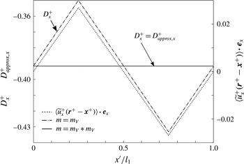
 $$\begin{eqnarray}\boldsymbol{D}_{approx}\triangleq \langle \widetilde{\boldsymbol{u}}\widetilde{T}\rangle _{m}=\langle \widetilde{\boldsymbol{u}}T^{\star }\rangle _{m}+\langle \widetilde{\boldsymbol{u}}\langle \unicode[STIX]{x1D6FE}_{f}(\boldsymbol{r}-\boldsymbol{x})\rangle _{m}\rangle _{m}\boldsymbol{\cdot }\unicode[STIX]{x1D735}T,\end{eqnarray}$$
is in general not spatially constant for a filter with
 $m=m_{G}\ast m_{V}$
, as this form of filter does not necessarily ensure that
 $\langle \widetilde{\boldsymbol{u}}\langle \unicode[STIX]{x1D6FE}_{f}(\boldsymbol{r}-\boldsymbol{x})\rangle _{m}\rangle _{m}=0$
. Besides, for this filter, the approximation
 $\boldsymbol{D}\simeq \boldsymbol{D}_{approx}$
is only permitted if the moment of the deviation velocity is sufficiently small,
 $\langle \widetilde{\boldsymbol{u}}(\boldsymbol{r}-\boldsymbol{x})\rangle _{m}\simeq 0$
, a condition which might be violated for some periodically developed flow fields.
In the case that the filter is based on
 $m=m_{C}\ast m_{V}\ast m_{V}$
, the moment of the velocity deviation field is exactly zero, i.e.
 $\langle \widetilde{\boldsymbol{u}}(\boldsymbol{r}-\boldsymbol{x})\rangle _{m}=0$
by analogy with (6.8), and the thermal dispersion source does become spatially constant:
 $$\begin{eqnarray}\boldsymbol{D}=\boldsymbol{D}_{approx}=\langle \widetilde{\boldsymbol{u}}T^{\star }\rangle _{m}.\end{eqnarray}$$
The equality
 $\boldsymbol{D}=\boldsymbol{D}_{approx}$
is a consequence of the fact that
 $T^{\star }$
and
 $\widetilde{T}$
are equal up to a constant for
 $m=m_{C}\ast m_{V}\ast m_{V}$
, according to (6.10) and (6.8).
The thermal tortuosity in the periodically developed conjugate heat transfer regime is obtained after substitution of (4.5) into (3.5):
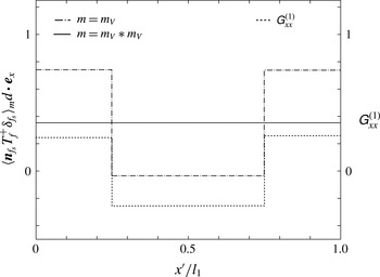
 $$\begin{eqnarray}\langle \boldsymbol{n}_{fs}T_{f}\unicode[STIX]{x1D6FF}_{fs}\rangle _{m}=(\unicode[STIX]{x1D642}_{m}^{(0)}(\boldsymbol{x}-\boldsymbol{x}_{0})+\unicode[STIX]{x1D642}_{m}^{(1)})\boldsymbol{\cdot }\unicode[STIX]{x1D735}T+\langle \boldsymbol{n}_{fs}T_{f}^{\star }\unicode[STIX]{x1D6FF}_{fs}\rangle _{m},\end{eqnarray}$$
where we again made use of the geometrical tensors of (2.7). Although
 $\unicode[STIX]{x1D642}_{m}^{(0)}=-\unicode[STIX]{x1D735}\unicode[STIX]{x1D716}_{fm}=0$
for any weighting function
 $m=m_{G}\ast m_{V}$
with
 $\bar{\unicode[STIX]{x1D6FA}}=\unicode[STIX]{x1D6FA}_{unit}$
for
 $m_{V}$
, we have in general
 $\unicode[STIX]{x1D642}_{m}^{(1)}\neq 0$
, as
 $\unicode[STIX]{x1D642}_{m}^{(1)}$
is spatially periodic over the unit cell domain for this form of weighting function. On the contrary, the weighting function
 $m=m_{C}\ast m_{V}\ast m_{V}$
does have the property that
 $\unicode[STIX]{x1D642}_{m}^{(0)}=\unicode[STIX]{x1D642}_{m}^{(1)}=0$
by (6.8) and therefore yields the following spatially constant thermal tortuosity term,
 $$\begin{eqnarray}\langle \boldsymbol{n}_{fs}T_{f}\unicode[STIX]{x1D6FF}_{fs}\rangle _{m}=\langle \boldsymbol{n}_{fs}T_{f}^{\star }\unicode[STIX]{x1D6FF}_{fs}\rangle _{m}=\langle \boldsymbol{n}_{fs}T_{s}^{\star }\unicode[STIX]{x1D6FF}_{fs}\rangle _{m}.\end{eqnarray}$$
The interfacial heat transfer term in the periodically developed heat transfer regime follows from substitution of (2.7) and (4.5) into (3.4), which results in
 $$\begin{eqnarray}\langle q_{fs}\unicode[STIX]{x1D6FF}_{fs}\rangle _{m}=-\langle \boldsymbol{n}_{fs}\boldsymbol{\cdot }(k_{f}\,\unicode[STIX]{x1D735}T_{f})\unicode[STIX]{x1D6FF}_{fs}\rangle _{m}=-\unicode[STIX]{x1D642}_{m}^{(0)}\boldsymbol{\cdot }k_{f}\unicode[STIX]{x1D735}T-\langle \boldsymbol{n}_{fs}\boldsymbol{\cdot }(k_{f}\,\unicode[STIX]{x1D735}T_{f}^{\star })\unicode[STIX]{x1D6FF}_{fs}\rangle _{m}.\end{eqnarray}$$
For any weighting function of the form
 $m=m_{G}\ast m_{V}$
with
 $\bar{\unicode[STIX]{x1D6FA}}=\unicode[STIX]{x1D6FA}_{unit}$
for
 $m_{V}$
, equation (6.3) is applicable, so the last term of (7.7) is constant and
 $\unicode[STIX]{x1D642}_{m}^{(0)}=-\unicode[STIX]{x1D735}\unicode[STIX]{x1D716}_{f}=0$
for this weighting function. In the periodically developed conjugate heat transfer regime, the interfacial heat transfer term is thus a constant scalar, whether the filter is based on
 $m=m_{G}\ast m_{V}$
or
 $m=m_{C}\ast m_{V}\ast m_{V}$
:
 $$\begin{eqnarray}\langle q_{fs}\unicode[STIX]{x1D6FF}_{fs}\rangle _{m}=-\langle \boldsymbol{n}_{fs}\boldsymbol{\cdot }(k_{f}\,\unicode[STIX]{x1D735}T_{f}^{\star })\unicode[STIX]{x1D6FF}_{fs}\rangle _{m}=-\langle \boldsymbol{n}_{fs}\boldsymbol{\cdot }(k_{s}\,\unicode[STIX]{x1D735}T_{s}^{\star })\unicode[STIX]{x1D6FF}_{fs}\rangle _{m}.\end{eqnarray}$$
Nevertheless, only for the weighting function
 $m=m_{C}\ast m_{V}\ast m_{V}$
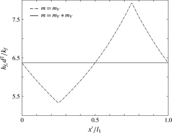
is the interfacial heat transfer coefficient of (3.4) spatially constant by (6.8), (6.6) and (6.7) and satisfies
 $$\begin{eqnarray}h_{fs}=\frac{\langle q_{fs}\unicode[STIX]{x1D6FF}_{fs}\rangle _{m}}{(\langle T^{\star }\rangle _{m}^{f}-\langle T^{\star }\rangle _{m}^{s})},\end{eqnarray}$$
where
 $\langle q_{fs}\unicode[STIX]{x1D6FF}_{fs}\rangle _{m}$
is given by (7.8).
The interfacial heat transfer coefficient of (7.9) was introduced as the heat transfer coefficient for the volume-averaged fluid and solid temperature in the studies of Alshare et al. (Reference Alshare, Strykowski and Simon2010a
) and Lopez Penha et al. (Reference Lopez Penha, Stolz, Kuerten, Nordlund, Kuczaj and Geurts2012), although we have shown that it requires the macro-scale temperature to be defined through the weighting function
 $m=m_{C}\ast m_{V}\ast m_{V}$
. This constant heat transfer coefficient depends on the same parameters as the periodic temperature, except the position vector
 $\boldsymbol{x}$
. For solid structures with a single geometric parameter
 $L_{ref}$
, the functional dependence of the heat transfer coefficient in the steady regime can be reduced to a dimensionless correlation between the Nusselt number (
 $h_{fs}L_{ref}^{2}/k_{f}$
), the Reynolds number based on the volume-averaged velocity (
 $\unicode[STIX]{x1D70C}_{f}\Vert \langle \boldsymbol{u}\rangle \Vert L_{ref}/\unicode[STIX]{x1D707}_{f}$
), the flow direction
 $\boldsymbol{e}_{s}$
, the Prandtl number of the fluid (
 $\unicode[STIX]{x1D707}_{f}c_{f}/k_{f}$
) and the conductivity ratio
 $k_{f}/k_{s}$
, at least if the heat source is spatially constant. For the unsteady periodically developed conjugate heat transfer regime, the time-averaged Nusselt number depends additionally on the fluid-to-solid heat capacity ratio (
 $\unicode[STIX]{x1D70C}_{f}c_{f}/(\unicode[STIX]{x1D70C}_{s}c_{s})$
) as well as the Strouhal number (
 $L_{ref}/(\unicode[STIX]{x1D70F}\Vert \langle \boldsymbol{u}\rangle \Vert )$
).
In summary, the interfacial heat transfer term is spatially constant in the periodically conjugate heat transfer regime for any filter based on the weighting function for volume averaging. The filter based on the weighting function of Quintard and Whitaker, which is in essence equivalent to a double volume average, ensures in addition that the interfacial heat transfer coefficient, as well as the thermal tortuosity and dispersion, are spatially constant in the periodically developed conjugate heat transfer regime, irrespective of the specific shape of the periodic solid structures.
The fact that these closure terms become spatially constant for the double volume-average filter indicates that there is no development any more from a macro-scale point of view. Therefore the double volume-average filter gives a macro-scale description in agreement with the physical interpretation of what it is called a developed regime, i.e. a regime in which the velocity and temperature profiles become similar for every unit cell and hence do not change from a macro-scale point of view. The physical interpretation of the closure terms for the simple volume-average filter is less clear, because the closure terms vary over the unit cell domain in the developed regime. The spatial gradients of these closure terms are mainly caused by the geometrical properties, the spatial moments, of the fluid–solid interface and they are not related to changes of the real macro-scale quantities such as the averaged flow velocity
 $\langle \boldsymbol{u}\rangle$
or the constant temperature gradient
 $\unicode[STIX]{x1D735}T$
.
8 Macro-scale conjugate heat transfer in an array of solid squares
In the following case study, a macro-scale description is given of the heat transfer between an array of solid squares having a uniform volumetric heat source and an incompressible fluid in which no volumetric heat generation takes place. This case study serves to support illustratively the theoretical derivations of the previous parts and exposes the essential features of the periodically developed conjugate heat transfer regime in solid structures.
Geometry of the square array and unit cell.

A single row of the two-dimensional array is depicted in figure 2 and consists of
 $\text{N}$
identical squares with side length
 $d$
, which are separated from each other by a distance
 $s_{x}$
along the horizontal axis
 $x$
. On the same figure,
 $s_{y}$
indicates the distance between two adjacent rows of the array. The checker-board pattern in figure 2 corresponds to a two-dimensional unit cell of the array with the lattice sizes
 $l_{1}$
and
 $l_{2}$
and coordinate axis
 $x^{\prime }$
. The values of all the parameters for this case study are summarized in table 1.
Case study parameters.
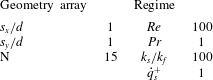
The velocity field through the single row of solid squares in figure 2 is computed for an imposed pressure drop
 $\unicode[STIX]{x0394}p$
between the inlet at
 $x=0$
and the outlet at
 $x=\text{N}l_{1}$
. The velocity field satisfies the no-slip condition at the boundaries of the solid squares. The temperature distribution over the single row of squares is calculated for a prescribed inlet temperature
 $T_{in}$
and a zero temperature gradient at the outlet. At the solid boundaries, the continuity of the temperature field as well as the interfacial heat flux, is imposed. As the velocity field and temperature distribution are resolved on only a single row of the array, they both are assumed to satisfy symmetry boundary conditions at
 $y=0$
and
 $y=l_{2}$
. Viscous dissipation is not considered and the uniform volumetric heat source in the solid is chosen such that
 $\dot{q}_{s}^{+}\triangleq \dot{q}_{s}d^{2}/(k_{s}\unicode[STIX]{x0394}T_{ref})=1$
, as we define
 $\unicode[STIX]{x0394}T_{ref}\triangleq \dot{q}_{s}d^{2}/k_{s}$
.
For numerically solving the steady Navier–Stokes flow and temperature equations, the finite-volume method is applied with the same discretization schemes as in our previous study (Buckinx & Baelmans Reference Buckinx and Baelmans2015a
). The finite-volume mesh for the square array in this case study consists of 937 500 quadrilateral cells of nearly equal size. For calculating the filtered flow and temperature distributions, the spatial filter operator is discretized by a number of 360 000 sample points following the approach of Buckinx & Baelmans (Reference Buckinx and Baelmans2015b
). Furthermore, all distributions are filtered assuming periodicity over the symmetry boundaries, so that the filtered quantities vary only in the direction of the unit vector
 $\boldsymbol{e}_{x}$
along the
 $x$
-axis of the square array.
Filtered dimensionless temperature distributions at the centreline
 $y=l_{2}/2$
of the square array.

Figure 3 shows the dimensionless temperature of the fluid and solid,
 $T^{+}\triangleq (T-T_{in})/\unicode[STIX]{x0394}T_{ref}$
, at the centreline of the square array. The fluid temperature rises in streamwise direction in front of each solid, as the solid conducts the heat from its internal heat source towards the fluid. In the immediate region after each solid, the presence of a wake with flow recirculation and less advective heat transport leads to a locally decreasing fluid temperature. Within the solid squares, the dimensionless temperature profile flattens, because the solid has a much higher heat conductivity than the fluid:
 $k_{s}/k_{f}=100$
, which explains why the temperature gradients within the solid region are much smaller than in the fluid region.
In this case study, the periodically developed conjugate heat transfer regime sets in after the second solid square at
 $x/d\simeq 4$
, causing the temperature profiles around the third to the second last solid square in figure 3 to become similar. The rapid onset of the periodically developed flow and heat transfer regime near the inlet is a typical observation for laminar incompressible flow of a fluid with
 $Pr=1$
at moderate Reynolds numbers. In this numerical experiment, we have chosen
 $Re\triangleq \unicode[STIX]{x1D70C}_{f}U_{ref}\,d/\unicode[STIX]{x1D707}_{f}=100$
, where
 $U_{ref}\triangleq \sqrt{\unicode[STIX]{x0394}p/\unicode[STIX]{x1D70C}_{f}}$
.
The fact that the heat transfer regime is periodically developed over the largest part of the square array also translates into a linearly increasing macro-scale temperature over the entire array, apart from the inlet and outlet region. More precisely, only the profiles of the intrinsically averaged fluid and solid temperatures
 $\langle T^{+}\rangle _{m}^{f}$
and
 $\langle T^{+}\rangle _{m}^{s}$
on figure 3, which are based on the weighting function
 $m=m_{V}\ast m_{V}$
, have a constant slope in the developed regime. The profiles of the intrinsically volume-averaged fluid and solid temperature
 $\langle T^{+}\rangle ^{f}$
and
 $\langle T^{+}\rangle ^{s}$
in figure 3 are clearly nowhere exactly linear. However, the difference between
 $\langle T^{+}\rangle ^{f}$
and
 $\langle T^{+}\rangle _{m}^{f}$
as well as the difference between
 $\langle T^{+}\rangle ^{s}$
and
 $\langle T^{+}\rangle _{m}^{s}$
, is small, indicating that the first-order volume-averaged spatial moments of the square solids are negligible. The small magnitude of these spatial moments is a consequence of the relatively high porosity
 $\unicode[STIX]{x1D716}_{f}=1-d^{2}/(l_{1}l_{2})=0.75$
of the square array, as can be seen from the expression (Quintard & Whitaker Reference Quintard and Whitaker1994c
; Wood Reference Wood2013) for the first-order spatial moment of the fluid indicator on the unit cell domain:
 $$\begin{eqnarray}\langle \unicode[STIX]{x1D6FE}_{f}(\boldsymbol{r}-\boldsymbol{x})\rangle \boldsymbol{\cdot }\boldsymbol{e}_{x}=\left\{\begin{array}{@{}ll@{}}(1-\unicode[STIX]{x1D716}_{f})x^{\prime }, & \displaystyle x^{\prime }\in \left[0,\frac{l_{1}-d}{2}\right]\\ \displaystyle (1-\unicode[STIX]{x1D716}_{f})\left[x^{\prime }-\frac{l_{1}}{d}\left(x^{\prime }-\frac{l_{1}-d}{2}\right)\right], & \displaystyle x^{\prime }\in \left[\frac{l_{1}-d}{2},\frac{l_{1}+d}{2}\right]\\ (1-\unicode[STIX]{x1D716}_{f})(x^{\prime }-l_{1}), & \displaystyle x^{\prime }\in \left[\frac{l_{1}+d}{2},l_{1}\right].\end{array}\right.\end{eqnarray}$$
It therefore seems that the simple volume-averaging operator succeeds in yielding a meaningful macro-scale temperature for this case. Nevertheless, we argue that the filter operator based on
 $m=m_{V}\ast m_{V}$
yields a more physically meaningful macro-scale temperature for the periodically developed conjugate heat transfer regime, and it does that for any porosity
 $\unicode[STIX]{x1D716}_{f}$
and any shape of the solid structures. The first argument is that the double-averaged fluid temperature
 $\langle T^{+}\rangle _{m}^{f}$
in a flow through solid structures subject to a periodic heat flux, resembles the linearly increasing fluid temperature in a channel without internal solids, but with walls subject to a constant heat flux (Shah & London Reference Shah and London1978).
Interfacial heat transfer coefficient over the unit cell domain for different weighting functions.

The second argument is that the filter operator based on the weighting function
 $m=m_{V}\ast m_{V}$
gives rise to an interfacial heat transfer coefficient
 $h_{fs}$
which is constant over space in the periodically developed regime. This property is illustrated in figure 4 and agrees with the notion that also the heat transfer coefficient in a channel with a constant wall flux is space independent in the fully developed flow and heat transfer regime (Shah & London Reference Shah and London1978). The space independence of the heat transfer coefficient for the weighting function of Quintard and Whitaker originates from the general principle that the difference between the curves of
 $\langle T\rangle _{m}^{f}$
and
 $\langle T\rangle _{m}^{s}$
is constant in the developed regime, as figure 3 confirms.
On the contrary, figure 4 reveals that the interfacial heat transfer coefficient
 $h_{fs}$
for the volume-averaged solid and fluid temperatures is a function of the position
 $x^{\prime }$
within the unit cell. For the weighting function
 $m_{V}$
, the heat transfer coefficient
 $h_{fs}$
thus varies together with the location where the difference between the volume-averaged temperatures of the fluid and solid,
 $\langle T\rangle ^{f}-\langle T\rangle ^{s}$
, is evaluated.
It is readily verified from (7.9) that the heat transfer coefficient for the weighting function
 $m_{V}$
, denoted by
 $h_{fs}(m_{V})$
, is related to the spatially constant heat transfer coefficient for the weighting function
 $m=m_{V}\ast m_{V}$
, denoted by
 $h_{fs}(m_{V}\ast m_{V})$
, through the formula
 $$\begin{eqnarray}h_{fs}(m_{V}\ast m_{V})=\left[\left\langle \frac{1}{h_{fs}(m_{V})}\right\rangle \right]^{-1}.\end{eqnarray}$$
We remark that the relative difference between
 $h_{fs}(m_{V}\ast m_{V})$
and
 $h_{fs}(m_{V})$
in figure 4 can be locally as much as 20 %, resulting in the conclusion that the weighting function has an important effect on the value of the interfacial heat transfer coefficient.
Thermal tortuosity for different weighting functions and first geometrical tensor over the unit cell domain.

Figure 5 gives the thermal tortuosity for the square array in the periodically developed conjugate heat transfer regime. The thermal tortuosity varies over the unit cell domain for the volume-averaging operator with the weighting function
 $m_{V}$
. As visualized in figure 5, the spatial dependence of the thermal tortuosity for
 $m_{V}$
is caused by the non-zero first geometrical tensor, whose component
 $\unicode[STIX]{x1D60E}_{xx}^{(1)}\triangleq \unicode[STIX]{x1D642}^{(1)}\boldsymbol{\cdot }\boldsymbol{e}_{x}\boldsymbol{e}_{x}$
is calculated numerically and agrees with its analytical expression
 $$\begin{eqnarray}\unicode[STIX]{x1D60E}_{xx}^{(1)}\triangleq \frac{\unicode[STIX]{x2202}}{\unicode[STIX]{x2202}x}\langle (\boldsymbol{r}-\boldsymbol{x})\unicode[STIX]{x1D6FE}_{f}\rangle \boldsymbol{\cdot }\boldsymbol{e}_{x}=\left\{\begin{array}{@{}ll@{}}(1-\unicode[STIX]{x1D716}_{f}), & \displaystyle x^{\prime }\in \left[0,\frac{l_{1}-d}{2}\right]\\ \displaystyle (1-\unicode[STIX]{x1D716}_{f})\left(1-\frac{l_{1}}{d}\right), & \displaystyle x^{\prime }\in \left[\frac{l_{1}-d}{2},\frac{l_{1}+d}{2}\right]\\ (1-\unicode[STIX]{x1D716}_{f}), & \displaystyle x^{\prime }\in \left[\frac{l_{1}+d}{2},l_{1}\right].\end{array}\right.\end{eqnarray}$$
In addition, figure 5 demonstrates that the weighting function of Quintard and Whitaker,
 $m=m_{V}\ast m_{V}$
, effectively results in a spatially constant tortuosity term, whose value is the average over the unit cell domain of the tortuosity term for the weighting function
 $m_{V}$
.
Thermal dispersion source for different weighting functions and volume-averaged spatial moment of the deviation velocity over the unit cell domain.

Figure 6 shows us that it is advantageous to define the macro-scale temperature through the double volume-averaging operator of Quintard and Whitaker for yet another reason: similar to the interfacial heat transfer coefficient and the thermal tortuosity, also the thermal dispersion source becomes spatially constant in the developed regime. The thermal dispersion source
 $D_{x}^{+}\triangleq \boldsymbol{D}\boldsymbol{\cdot }\boldsymbol{e}_{x}/(U_{ref}\,\unicode[STIX]{x0394}T_{ref})$
then equals
 $D_{approx,x}^{+}\triangleq \langle \widetilde{u}^{+}\widetilde{T}^{+}\rangle _{m}\boldsymbol{\cdot }\boldsymbol{e}_{x}$
, with
 $m=m_{V}\ast m_{V}$
.
As figure 6 shows, when the volume-averaged temperature is taken as macro-scale temperature, a dependence of the thermal dispersion source on the unit cell coordinate
 $x^{\prime }$
is induced by the non-zero volume-averaged spatial moment of the deviation velocity,
 $\langle \widetilde{\boldsymbol{u}}^{+}(\boldsymbol{r}^{+}-\boldsymbol{x}^{+})\rangle \boldsymbol{\cdot }\boldsymbol{e}_{x}\boldsymbol{e}_{x}\triangleq \langle \widetilde{u}_{x}(\boldsymbol{r}-\boldsymbol{x})\rangle \boldsymbol{\cdot }\boldsymbol{e}_{x}/(U_{ref}\,d)$
.
We would like to emphasize that all the closure terms for the single and double volume-average filter in figures 4–6 have been numerically calculated first from the filtered temperature and velocity distributions through their definitions (3.3)–(3.5). Afterwards, we have verified that these values agree with the exact closure equations of § 7, which required us to solve the periodic temperature part on the unit cell domain via (4.10)–(4.13) and (5.2). The unit cell closure equations of § 7 depend on the velocity field on the unit cell domain, which was numerically reconstructed from the constant filtered velocity field
 $\langle \boldsymbol{u}\rangle _{m}=\langle \boldsymbol{u}\rangle _{m}$
in the developed regime via the exact closure equations of Buckinx & Baelmans (Reference Buckinx and Baelmans2015b
).
Comparison of deviation temperature profiles around the eighth solid square (solid lines) with unit cell simulation (circle markers).

The last illustration, figure 7, gives the profiles of the deviation temperature for
 $m=m_{V}\ast m_{V}$
within the unit cell whose centroid coincides with the centre of the eighth solid square. These profiles are obtained in two ways. First, the deviation temperature profiles are calculated via their definition, equation (2.4), by filtering the full temperature distribution. Second, the deviation temperature is reconstructed exactly by solving just the periodic temperature part on the unit cell domain via the equality
 $\widetilde{T}=T^{\star }-\langle T^{\star }\rangle _{m}^{f}\unicode[STIX]{x1D6FE}_{f}-\langle T^{\star }\rangle _{m}^{s}\unicode[STIX]{x1D6FE}_{s}$
that follows from (6.10). The reconstruction of the micro-scale temperature details
 $\widetilde{T}^{+}$
in the periodically developed regime requires only knowledge of the unit cell geometry, the parameters of the flow and heat transfer regime,
 $k_{s}/k_{f}$
,
 $Pr$
and
 $Re$
and finally the heat source
 $\dot{q}^{+}$
. The reconstruction of the deviation part of the volume-averaged temperature would necessitate in addition the calculation of the first-order spatial moments, as well as the first geometrical tensor and the volume-averaged spatial moment of the deviation velocity.
In conclusion, we have illustrated in this case study that both the thermal closure terms and the deviation temperature are exactly predicted in the periodically developed conjugate heat transfer regime by solving the periodic temperature part on the unit cell domain via the exact closure equations of § 7. In principle, also the filtered temperature distributions in figure 3, which are obtained by filtering the DNS results, thus could have been exactly reconstructed in the developed region
 $x/d\simeq 4\ldots 26$
, if the exact boundary conditions for the filtered temperature equations (3.1) and (3.2) were known. However, the temperature conditions at the onset of the periodically developed regime,
 $\langle T\rangle _{m}^{f}|_{\boldsymbol{x}_{0}}$
and
 $\langle T\rangle _{m}^{s}|_{\boldsymbol{x}_{0}}$
, which determine the constant
 $\langle \overline{T^{\star }}\rangle$
, are in general unknown for every spatial averaging operator, whether a traditional volume average or a double volume average is chosen.
9 Conclusions
The macro-scale heat transfer between an incompressible flow and spatially periodic solid structures can be modelled via spatially averaged or ‘filtered’ temperature equations containing three closure terms: the thermal dispersion source, the thermal tortuosity and the interfacial heat transfer. The form of these closure terms depends on the flow and heat transfer regime, but also on the spatial filter that defines the macro-scale temperature. In the periodically developed conjugate heat transfer regime, all the solid structures have the same interfacial heat flux distribution, so that the closure terms can be governed by resolving the periodic part of the temperature field on a unit cell of the solid structures. For a simple volume-average filter, as in the VAT, the closure terms in the periodically developed regime vary with the position within the unit cell. Nevertheless, the spatial dependence of the closure terms for the volume-averaged temperature has been neglected by previous studies. On the other hand, for a double volume-average filter based on the weighting function of Quintard and Whitaker, the thermal dispersion source, the thermal tortuosity as well as the interfacial heat transfer coefficient and macro-scale temperature gradient are all spatially constant. It is therefore concluded that the appropriate filter for the macro-scale temperature in the periodically developed conjugate heat transfer regime is equivalent to a double volume average. To the authors’ knowledge, the correct form of the closure terms and an appropriate definition of the macro-scale temperature in the periodically developed heat transfer regime have not been given before.
Acknowledgement
This work is sponsored by the Institute for the Promotion of Innovation through Science and Technology in Flanders (IWT-Vlaanderen). Numerical results in this paper were obtained using FVMLab, a C
 $++$
/Matlab-based finite volume solver package developed by F. Rogiers and G.B. For all numerical results we used the infrastructure of the VSC – Flemish Supercomputer Center, funded by the Hercules foundation and the Flemish Government – department EWI.