Introduction
The indentation size effect (ISE) has been studied for two decades, with the most accepted model of the physical origin presented by Nix and Gao [Reference Nix and Gao1]. In the context of examining the ISE in thin films, the terms “intrinsic” and “extrinsic” size effect were introduced by Ngan and Ng [Reference Ngan and Ng2] to distinguish between the indentation response of the film itself versus the combined response of the film/substrate system. Following a slightly modified form of that nomenclature, here we compare and contrast the intrinsic and extrinsic ISE in high-purity and carbon-doped iron. In this context, we use the terms intrinsic and extrinsic to distinguish between the effect of the indenter geometry–induced plastic strain gradient [Reference Nix and Gao1], as observed in well-annealed, single crystal surfaces, and the effect(s) of preexisting defect structures in the same material, respectively. Based on that distinction, the depth-dependent hardness, H, as measured by Berkovich nanoindentation experiments, is used to interrogate the structure–property relationship of specific defect structures that show extrinsic size effects. The four cases analyzed are (i) three different well-annealed, single-crystal Fe surfaces (intrinsic ISE), (ii) a deformed surface layer for one of the same grains, (iii) a “cylinder” of plastic deformation produced by a linear array of shallow indents for the same grain, and (iv) four random grain boundaries of varying tilt/twist character. This paper does not attempt to address the fundamental mechanisms responsible for the details of the intrinsic ISE in well-annealed, low–dislocation density materials. Instead, the paper examines how the depth-dependent H may be correlated with the configuration and strengthening properties of preexisting defects.
The analysis implemented here adopts the mathematically transparent, mechanistic model of Nix and Gao [Reference Nix and Gao1] for ISE, which is based on the widely accepted concept of Taylor hardening. The analysis is then extended with a strain gradient plasticity (SGP) model, which includes spatial dependence of plastic strain. In the Nix–Gao model [Reference Nix and Gao1], the Taylor hardening concept was combined with the concept of geometrically necessary dislocations (GNDs) [Reference Ashby3] that would be required to accommodate the gradient in plastic strain imposed by a geometrically self-similar indenter tip such as the Berkovich. The GNDs were considered as additive to the statistically stored dislocations (SSD) in the Taylor expression, where the SSD are due to the indentation characteristic strain. Both the SSD and GND densities were considered as being uniform (averaged) throughout the indentation volume [Reference Nix and Gao1]. To explain decreasing hardness with increasing depth, this model proposes that GND have an increase in spacing as the indentation depth increases, causing a reduction in Taylor hardening. The Nix–Gao model for indentation of initially defect-free material relates the hardness, H, to the indentation-induced averaged dislocation density as,
 $$H = {H_0}\sqrt {1 + {{{h^*}} \over {{f^3}h}}} \quad ,$$
 $${H_0} = 3\sqrt 3 \alpha Gb\sqrt {{\rho _{{\rm{SSD}}}}} \quad ,$$
 $${h^*} = {{3\;{{\tan }^2}\;\theta {f^2}} \over {2b{\rho _{{\rm{SSD}}}}}}\quad ,$$
 $${\rho _{{\rm{GND}}}} = {{3\;{{\tan }^2}\;\theta } \over {2bfh}}\quad ,$$
where H 0 is the bulk hardness free of GNDs; h* is the characteristic depth; f is a material-dependent parameter introduced by Durst et al. [Reference Durst, Backes and Goken4], which attempts to provide a more accurate estimate of the hemispherical volume containing the GNDs; α is a constant taken to be 0.5, G is the shear modulus; b is the Burgers vector; ρSSD and ρGND are the SSD and GND densities, respectively; and θ is the angle between the indenter and the undeformed surface.
Literature describing how the ISE could be used to determine the defect configuration and/or structure–property relationships in the presence of preexisting defects is relatively rare. Specific examples taking this approach can be found in the grain boundary indentation literature and in the analysis of thin film indentation [Reference Ngan and Ng2, Reference Hou, Bushby and Jennett5, Reference Voyiadjis and Yaghoobi6]. In a manner that is directly related, changes in the ISE due to subsurface dislocation gradients created by mechanical polishing have been examined in high-purity Ni [Reference Wang7]. In this case, over indentation depths from 400 to 800 nm, it was shown that a plot of H 2 versus 1/h for mechanically polished Ni has a larger slope, ∝h*, than the equivalent plot for mechanically polished Ni that has been subsequently electropolished [Reference Voyiadjis and Yaghoobi6]. Similarly, as suggested by Pharr et al. [Reference Pharr, Herbert and Gao8], differences in the measured h* of pure Cu between different research groups [Reference McElhaney, Vlassak and Nix9, Reference Liu and Ngan10] can be attributed to variations in the ISE due to the effect of mechanical polishing. However, attempts to quantitatively relate this variance in the ISE to the defect configuration within the stressed volume have not been made. Examination of the ISE in work-hardened Cu (uniform macroscopic strain) versus well-annealed Cu was studied by Poole et al. [Reference Poole, Ashby and Fleck11], where it was shown that cold work does not affect the slope of the H–h curve but does increase the magnitude of H. As a counterexample to Poole et al. [Reference Poole, Ashby and Fleck11], Backes et al. [Reference Backes, Huang, Goken and Durst12] reported a reduction in the ISE as measured in 10% prestrained Cu compared with well-annealed Cu. In contrast to the work by Poole et al. [Reference Poole, Ashby and Fleck11] and Backes et al. [Reference Backes, Huang, Goken and Durst12], where the deformation is relatively homogeneous, the variance in ISE reported in Reference WangRefs. 7, Reference Liu and Ngan10, and Reference Soman, Herbert, Aifantis and Hackney13 and reported herein is attributed to gradients in the subsurface damage and, thus, is considered a direct result of the inhomogeneity in the preexisting forest dislocation (FD) density near the free surface.
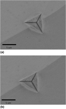
Despite a rapidly expanding pool of literature on grain boundary indentation and the ISE, it does not appear the two have been studied or analyzed in the manner presented here [Reference Hou, Bushby and Jennett5, Reference Voyiadjis and Yaghoobi6, Reference Rester, Motz and Pippan14, Reference Jung, Lee and Park15]. Specifically, it is found that most published Berkovich indentation studies have focused on “remote” indentation, as shown in Fig. 1(a), where the indenter tip is a significant distance from the grain boundary and, thus, the H variation with h is studied as the plastic zone approaches the grain boundary. Remote indentation with the face of the pyramidal indenter parallel to the grain boundary would seem to accentuate analysis of slip transmission across the boundary, as the angle of the indenter face is most acute here and the rate of approach of the indenter face with increasing h is minimized. In the analysis presented here, the goal is to place the pyramidal Berkovich indenter tip as close to the grain boundary as possible. Due to constraints imposed by the optical microscope and screw-driven stages, the targeting accuracy is ∼±1 μm. Within this range, deviations in the precise placement of the indenter tip are deemed acceptable, provided the tip is oriented such that the wedge of the pyramid formed by the intersection of the pyramid faces is approximately perpendicular to the grain boundary plane trace, as shown in Fig. 1(b). Due to the obtuse angle of the indenter geometry at the face intersections, this orientation effectively places a wedge across the grain boundary plane, inducing nearly simultaneous initiation of deformation in the adjacent grain at very small indentation depths. This contact orientation produces H–h curves, which typically do not show a discontinuity (pop-in) at indentation depths >100 nm, as compared with those shown in Refs. Reference Aifantis and Ngan16, Reference Soer, Aifantis and Hosson17, and Reference Aifantis, Deng, Shibata, Tsurekawa, Lejcek and Hackney18. However, the H–h behavior in this orientation does show an increase in H above that of both adjacent grain interiors and a unique extrinsic ISE, again quite distinguishable from the intrinsic ISE for either of the adjacent grains.
(a) Backscatter image channeling contrast of the Berkovich pyramid geometry referred to as local grain boundary indentation, with the wedge of the pyramid cutting across the boundary at shallow depths, inducing plastic deformation in both grains without the necessity of slip transmission across the boundary. (b) Backscatter image channeling contrast of the Berkovich indenter geometry typically used to study slip transmission across the grain boundary, where slip transmission occurs at depths prior to the surface shape change of the remote grain (accepted for publication).

It is proposed that the indentation geometry primarily utilized here [Fig. 1(b)] would tend to emphasize a grain boundary strengthening effect that occurs at plastic strain significantly beyond the yield point, as originally envisioned by Ashby [Reference Ashby3] and correlated with the concept of plastic strain anisotropy across the grain boundary [Reference Taylor19]. It is noted that there has been some work in the literature relating nanoindentation results to the Ashby proposal of plastic strain incompatibility, although not utilizing the same approach as in this paper. Vachhani et al. [Reference Vachhani, Doherty and Kalidindi20] used spherical nanoindentation near grain boundaries of deformed polycrystalline Al to examine local hardening at the grain boundaries due to prior macroscopic deformation. Vachhani et al. [Reference Vachhani, Doherty and Kalidindi20] correlated this local hardening to plastic anisotropy through the Taylor factor mismatch across the boundary. It was not the focus of the authors [Reference Vachhani, Doherty and Kalidindi20] in this previous work to examine grain boundary indentation in well-annealed samples or any variance in the ISE between indentation within a well-annealed grain interior and indentation at a well-annealed grain boundary, as in the current paper, but rather to expose the localized hardening at the grain boundary due to macroscopic deformation. Nevertheless, the Vachhani et al. [Reference Vachhani, Doherty and Kalidindi20] findings are important to the interpretation presented in this paper.
As this paper utilizes the Nix–Gao [Reference Nix and Gao1] approach to interpret the extrinsic ISE due to grain boundaries and non-uniform dislocation distributions, it is useful to examine other works that are related to this approach. The works presented by Hou et al. [Reference Hou, Bushby and Jennett5] and Jung et al. [Reference Jung, Lee and Park15] have the most in common with the ISE analysis presented here. Of particular interest, Jung et al. utilized a modified Nix–Gao relationship [Eqs. (1a)–(1d)] to analyze the ISE contribution of grain boundaries but examined the remote indentation results of Yang et al. [Reference Yang and Vehoff21] obtained from the center of Ni grains rather than local to the grain boundary. Another relevant grain boundary investigation is that of Xiao et al. [Reference Xiao, Terentyev, Chen, Yua, Chen, Bakaev and Duan22], wherein the remote indentation strengthening effect is also analyzed using the Nix–Gao relationship. Xiao et al. proposed that the grain boundary effectively reduces the volume of the plastic zone without affecting the number or length of the intrinsic GNDs, thus increasing the dislocation density that results in Taylor hardening [Reference Xiao, Terentyev, Chen, Yua, Chen, Bakaev and Duan22]. Although the approach of Xiao et al. is similar to the treatment here, the analysis is limited to slip transmission induced by remote indentation [Fig. 1(a)] and does not specifically analyze “local” indentation [Fig. 1(b)] and plastic incompatibility at the grain boundary. In contrast to these investigations, we propose that aspects of the originality of the experimental observations presented here are associated with the orientation, asymmetry, and location of the Berkovich indentation with respect to the grain boundary plane. As such, our analysis of experimental observations focuses on the abrupt imposition of equivalent stress above the yield stress associated with Berkovich indentation at the grain boundary rather than the gradual increase in stress with increasing h at the boundary plane related to remote Berkovich indentation or local spherical indentation [Reference Pathak, Michler and Wasmer23].
Previously, we proposed that changes in the slope of H 2 versus 1/h can be utilized to study an FD density gradient induced by mechanical polishing through direct comparisons to the H measured in the same but well-annealed grain [Reference Soman, Herbert, Aifantis and Hackney13]. To support the proposed concept of using the extrinsic ISE to examine the relevant microstructures, here we first present new results that reinforce our previous findings. Examination of this phenomenon leads to the rather simple, but previously unexplored, concept that the averaged spatial variation of the FD density (due to mechanical polishing) with depth can contribute to the nonlinear H 2 versus 1/h behavior. The paper then extends this defect-related extrinsic ISE to the analysis of a cylinder of plastic deformation produced by a row of shallow indents. These two cases of local defect analysis are then compared with grain boundary mechanical behavior as exposed by an ISE different from the intrinsic ISE of the adjacent grain interiors.
To interpret the ISE and capture the effect of GNDs, a continuum SGP model is employed. Such frameworks, initially proposed by Aifantis [Reference Aifantis24] consider the gradient of the plastic strain as an independent variable and demonstrated by Fleck et al. [Reference Fleck, Muller, Ashby and Hutchinson25] and Aifantis [Reference Aifantis26] are able to capture the scale of the microstructure, allowing the interpretation of size effects. More recently, interface energy terms within gradient plasticity developed by Aifantis and Willis [Reference Aifantis and Willis27, Reference Aifantis and Willis28] have been able to account for the existence of grain boundaries during nanoindentation experiments [Reference Aifantis and Ngan16]. The present experiments are able to further capture the effect of grain boundaries and provide additional qualitative understanding of the mechanically induced interface energy terms, while at the same time probing further into the ISE effect.
Experimental procedures
Cylindrical disks of high-purity (99.999%) Fe 10 mm in diameter and 4 mm thick were annealed for over 40 h at 800 °C in a hydrogen atmosphere to create grain sizes up to 2 mm in diameter. The large grain size is necessary to obtain multiple indentations at a spacing of >20 µm along the grain boundary. Following the long-term anneal, samples were mechanically polished using grinding papers ranging from P-800 to P-2400. Subsequently, the specimens were sequentially polished using 1, 0.3, and 0.05 μm alumina slurries. Following the mechanical polishing, plasma etching was performed to remove any contaminants, such as, but not limited to, mineral deposits and organic residue, left behind from the mechanical polishing and washing process. The etching was performed using the Anatech Hummer 6 (Hayward, California). Following plasma etching, the specimens were heat treated in a hydrogen atmosphere at 850 °C for 4–5 h. Annealing at 62% of the absolute melting temperature, the goal was to eliminate any remaining gradient in the dislocation density relative to the free surface and remove any carbon-based contamination. After annealing, the specimens were cooled in an Ar atmosphere to ensure excess hydrogen was removed from the free surface, as the literature shows that hydrogen effects on Fe yield point [Reference Rogers29] and hydrogen desorption from Fe dislocation and grain boundary “traps” occurs at baking temperatures less than 250 °C [Reference Song, Suh and Bhadeshia30].
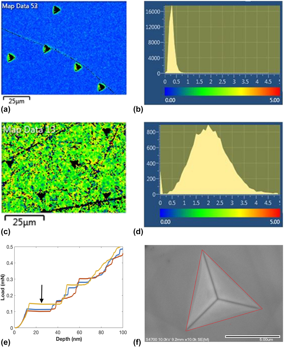
After the H2:Ar annealing, ion milling was performed using the JEOL IB-19500CP (Peabody, Massachusetts) cross-section polisher. Operating with a voltage of 6.5 kV for 10 min followed by the fine mode milling, the low-energy argon beam was used to remove any contaminants inadvertently deposited on the surface during heat treatment. The assessment of the quality and structure of the free surface region in relation to this sample preparation process is considered a critical aspect of the experimental procedure for the nanoindentation study. Specimen surfaces were characterized using an Oxford electron backscatter diffraction (EBSD) system interfaced with the FEI XL40 environmental scanning electron microscope. EBSD images and kernel average misorientation (KAM) maps show the mechanically polishing, followed by plasma etching, annealing, and ion milling produces surfaces [Figs. 2(a) and 2(b]) with very low dislocation density compared with the unannealed mechanically polished KAM [Figs. 2(c) and 2(d]). The step size used for the KAM analysis was 0.5 μm with a filter size of 3 × 3 and a threshold angle of 5°.
(a) Sample preparation methodology produces a large grain (>1 mm) sample with excellent quality map EBSD images, (b) KAM distribution plot for well-annealed surfaces, and (c) KAM image for mechanically polished surfaces that will include a contribution from the excess dislocations produced from the polish. (d) KAM plot for the mechanically polished surface and (e) well-annealed grain interior load:displacement curves showing the displacement discontinuity generally expected for dislocation nucleation processes at surfaces with a very low preexisting dislocation density. (f) Secondary electron SEM image of a grain interior indentation. The contact area is measured from the image and compared with the area function calculation from the reported indentation depth. The difference in the area measurement and area function result of 2.4% indicates the approximation of h = h c involves only a small error.
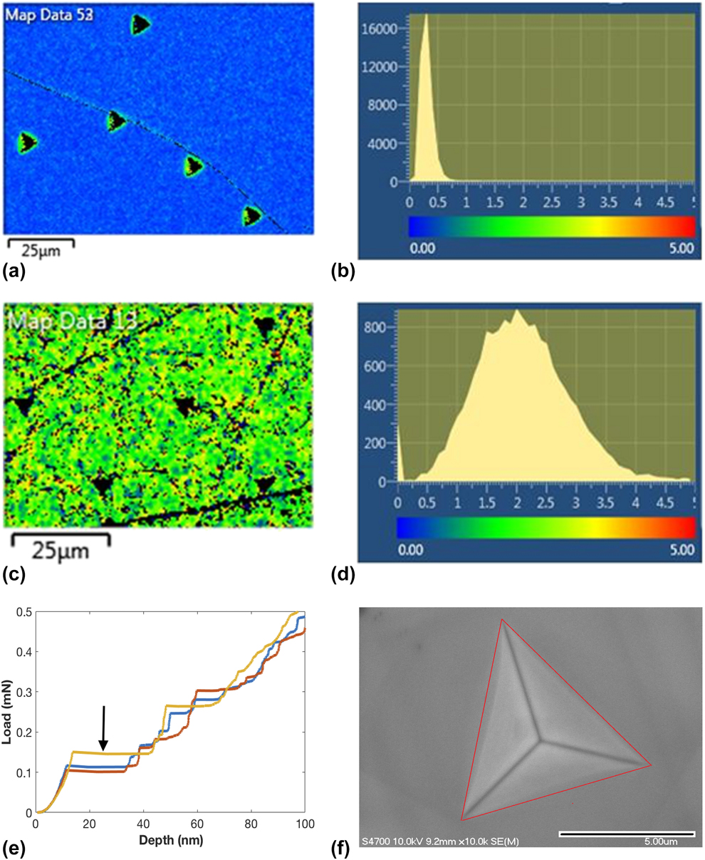
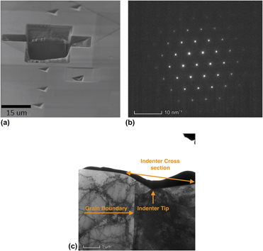
Additional evidence to support this claim of low surface dislocation density is presented in Fig. 2(e), which shows shallow indentation depth pop-in behavior that is indicative of dislocation nucleation in the nearly dislocation-free surface. Note that Fig. 2(a) is a KAM map of Berkovich indentations along a grain boundary and thus indicates that the indentation contact area is much smaller than the grain size. The free surface and grain boundaries were studied in the annealed state, the deformed state, and also after being doped with carbon in the annealed state. Carbon doping allows the comparison of indentation results at the same grain boundary, with and without carbon. The carbon doping was carried out by encapsulating the high-purity Fe specimen discs and 0.01 mg of polyethylene as a carbon source inside an evacuated quartz tube that was subsequently heat treated at 500 °C for 3 h. This heat treatment time and temperature give a carbon diffusion length of ∼3 × 10⁻⁴ m and a maximum average carbon concentration within the diffusion zone of ∼0.002 weight percent. Using a focused beam of high-energy (30 kV) gallium ions, the Hitachi FB-2000A (Krefeld, Germany) focused ion beam (FIB) mill was used to create FIB cross sections of residual hardness impressions [Fig. 3(a)] for analysis in the FEI (Einhoven, Netherlands) 200 kV Titan Themis scanning transmission electron microscope (S-TEM). As shown in Fig. 3(b), the grain boundary is perpendicular to the free surface. The diffraction pattern represented in Fig. 3(c) shows no evidence of additional phases such as Fe3C that could have formed during carbon doping.
(a) FIB cut on grain boundary. (b) Fe electron diffraction shows no evidence of carbides or other 2nd phase ppt. (c) Local indentation grain boundary cross section indicates grain boundary plane approximately perpendicular to the surface.

Nanoindentation experiments were performed using a diamond Berkovich indenter tip and the iNano (Nanomechanics Inc.—KLA Tencor, Oak Ridge, Tennessee). The loading rate,  $\dot{P}$, was controlled such that
 ${{\dot{P}} / P}$ was held constant at 0.2 1/s. Analysis of the ISE was performed from experiments terminated at a maximum load of 24 mN. Rather than calculating the contact depth by subtracting the elastic deflection of the surface (as prescribed by the Oliver–Pharr model), here we take the contact depth, h c, to be in the original plane of the surface, i.e., h c = h. As justification for this simplification, Fig. 2(f) shows a secondary electron SEM image of a representative residual hardness impression from an experiment performed to the maximum load used in this study of 24 mN. Indicative of well-annealed iron’s significant capacity to work harden, the image shows no significant evidence of pileup, as the contact edges connecting the 3 corners are relatively straight, smooth lines that appear to be in the original plane of the surface. The unique, minor deviations in linearity observed along each of the 3 faces are taken to be the result of anisotropy effects. Upon confirmation of the microscope’s x–y calibration, the measured projected contact area is compared with the calculated contact area (outlined by the red boundary) and is found to be greater than the calculated area by 2.4%. This small degree of error is consistent with the predictions of Lucas [Reference Lucas31]. We note that since the ISE forces the loss of geometric self-similarity of the contact, the error imposed by the simplified definition may increase inversely with indentation depth. However, the simplified definition of the contact area is further justified for two reasons. First, this investigation focuses on the measured difference between the intrinsic and extrinsic size effect in alpha iron rather than the absolute value of the measured hardness. In this case, the error in the h c = h approximation is associated with the difference in the elastic deflection between the intrinsic versus extrinsic ISE and not the absolute value of the elastic deflection. Second, due to the test specimen’s high ratio of E/σy (211 GPa/50 MPa = 4220), accurate measurements of the elastic contact stiffness as a continuous function of depth and, hence, accurate estimates of the elastic deflection of the surface are fraught with experimental challenges, such as, but not limited to, intermittent contact [Reference Pharr, Strader and Oliver32, Reference Merle, Maier-Kiener and Pharr33, Reference Herbert, Hackney, Dudney and Phani34], plasticity effects [Reference Merle, Maier-Kiener and Pharr33, Reference Herbert, Hackney, Dudney and Phani34, Reference Herbert, Sudharshan and Johanns35], time-dependent flow [Reference Herbert, Hackney, Dudney and Phani34, Reference Herbert, Sudharshan and Johanns35, Reference Oliver and Pharr36], and extrapolation of the frame stiffness [Reference Herbert, Hackney, Dudney and Phani34]. Based on the uncertainty associated with these potential experimental problems and the result of Fig. 2(e), we have adopted this simplified definition of the contact depth. Accordingly, the elastic deflection of the surface is ignored and H can, therefore, be calculated as a continuous function of depth based solely on the acquired P–h data [Reference Lucas31, Reference Herbert, Hackney, Dudney, Thole and Phani37]. While ignoring the elastic deflection clearly reduces the accuracy of the estimated hardness, it is not immediately clear the error imposed by the simplified definition is any worse than the potential error imposed by the experimental challenges mentioned above. Moreover, any intermittent contact, which is particularly difficult to eliminate at small depths without paying a very significant penalty in the signal–to-noise ratio, would completely eliminate the opportunity to measure the intrinsic ISE.
Experiments were performed with two indenter orientations relative to the grain boundary and within the adjacent grain interiors. Figure 1(a) is a backscatter scanning electron microscopy (SEM) image of a remote grain boundary indentation with the indenter tip positioned ∼2 µm from the grain boundary and the flat face of the indenter parallel to the boundary. In this orientation, plastic deformation is induced in the indented grain first and dislocations can be treated as being pushed against the grain boundary as the plastic zone expands with increasing h. Alternatively, Fig. 1(b) shows a local grain boundary indentation, wherein the indenter tip is positioned less than 0.5 µm from the grain boundary with the “wedge” of the indenter being perpendicular to the grain boundary plane. In this orientation, there is a near simultaneous deformation of both grains adjacent to the boundary due to direct contact of the indenter with the grain surfaces. A unique difference in the extrinsic ISE was observed for these two different indenter-grain boundary orientations, as shall be discussed in the Analysis section. The intrinsic ISE was determined using 20 indentations from the grain interiors adjacent to the studied boundaries.
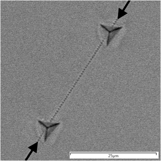
Preexisting deformation gradients relative to the free surface of the H2:Ar Fe were intentionally created to examine the validity of using changes of the measured ISE relative to the intrinsic ISE of a well-annealed H2:Ar heat-treated grain. A “one-dimensional" deformation gradient with a dislocation density gradient perpendicular to the surface was produced by mechanically polishing the surface using a coarse grit of P-800, P-1200, and P-2400 and fine polish using 1, 0.3, and 0.05 μm alumina [Reference Soman, Herbert, Aifantis and Hackney13]. Due to cell wall formation and other plastic inhomogeneities, we realize that the resulting dislocation density will not uniformly decrease with increasing depth below the surface. Rather, here we assume changes in the average dislocation density within the plastic zone with increasing h, which effectively serves as a smoothing function, defines the gradient. To complement our examination of changes in the ISE brought about by a one-dimensional deformation gradient, we created a two-dimensional gradient by placing a closely spaced linear array of 250 small indentations (residual depth of 100 and 700 nm spacing) within the grain interior of a well-annealed specimen. This geometry is expected to produce a cylinder of high dislocation density by virtue of the overlapping the plastic zones of the closely spaced, shallow indentations. In this case, the dislocation density gradient will be both perpendicular to the surface and perpendicular to the linear array of indentations. To examine the effect of this multidimensional deformation gradient, indentation experiments were performed local to the array, as shown in Fig. 4, where the arrows identify the linear array of indentations.
Backscatter SEM image for a linear array of closely spaced, shallow indentations with deeper indentations probing the properties using the local geometry similar to Fig. 1(b).

Results and discussion
Grain interior indentation results
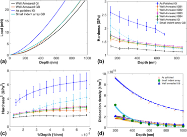
It is observed from the load–depth (P–h) curves in Fig. 5(a) and averaged hardness versus depth (H–h) profile plots in Fig. 5(b) that the H for the “as-polished” 〈120〉 grain surface and indentation row deformation is significantly greater than that for the fully annealed grain interior, especially at small indentation depths. It may also be seen that the H at the grain boundary for the well-annealed sample is greater than that for the corresponding adjacent grain interior of the well-annealed sample. The increase in H for the as-polished grain interior and indentation row is expected on the basis of FD strengthening (work hardening) of the surface due to mechanical polishing [Reference Samuels38] and the overlapping plastic strain fields of the closely spaced, shallow indentations. The increase in H at the grain boundary is expected due to grain boundary strengthening mechanisms interacting with the indentation plastic deformation. This paper intends to go beyond these simple concepts to examine how the ISE at these defect structures can provide additional information concerning the deformation mechanism and defect distribution. The degree of the ISE can be determined by noting the decrease in H with depth or the increase in H 2 with 1/h [Figs. 5(b) and 5(c)]. As seen in Figs. 5(b) and 5(c), the ISE is most obvious for the unannealed, mechanically polished specimen.
(a) Representative P–h curves for mechanically polished (deformed) grain surface, well-annealed grain surface, well-annealed grain boundary surface intersection, and line source indentation. (b) Plot between hardness and depth (averaged from 20 H versus h curves at each condition) for all the processing conditions, indicating presence of ISE as a function of processing condition. The hardness of the grain boundary is also shown on the plot for comparison. (c) Nix–Gao based H 2 versus 1/h plots for all the processing conditions. (d) Calculated FD density [Eq. (2)] for as polished surface, 4 grain boundaries as well as line source indentations.
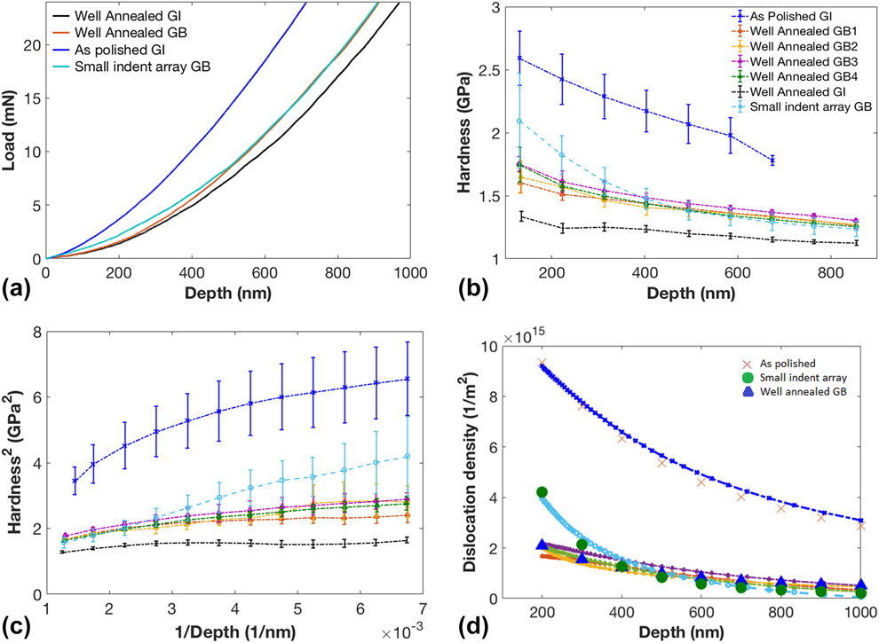
According to the Nix–Gao model, H 2 versus 1/h should be linear, with the slope corresponding to the decrease in GND density with depth. Only the well-annealed sample approaches linear behavior. Previous work [Reference Soman, Herbert, Aifantis and Hackney13] has suggested that the experimental observations of the hardening effect of the polishing FD density averaged over the indentation volume,  $\overline {{\rho _{{\rm{FD}}}}}$, can be accounted for by rewriting Eq. (1) as follows:
 $${H^2} = {H_0}^2\left( {1 + {{\overline {{\rho _{{\rm{FD}}}}} } \over {{\rho _{{\rm{SSD}}}}}} + {{{h^*}} \over {{f^3}h}}} \right)\quad .$$
Equation (2a) is an extension of the concept introduced by Poole et al. [Reference Poole, Ashby and Fleck11] that the preexisting dislocation density in a sample can be accounted for by a linear addition with the dislocations density produced by indentation. However, it is here considered that  $\overline {{\rho _{{\rm{FD}}}}}$ for the surface deformation due to polishing or from the row of shallow indentations is a function of h. Solving Eq. (2a) explicitly for
 $\overline {{\rho _{{\rm{FD}}}}}$ as a function of indentation depth gives
 $${{{H^2} - {H_0}^2\left( {1 + {{{h^*}} \over {{f^3}h}}} \right)} \over {{{\left( {3\sqrt 3 \alpha Gb} \right)}^2}}} = \overline {{\rho _{{\rm{FD}}}}} \quad ,$$
where H has been measured as function of h. The functional form for  $\overline {{\rho _{{\rm{FD}}}}}$ can be determined by comparing Eq. (2b) with cold worked and annealed H–h data in Fig. 5(c). Examining the annealed grain interior data first, such that
 $\left[ {{{\overline {{\rho _{{\rm{FD}}}}} } / {{\rho _{{\rm{SSD}}}}}}} \right]\; \sim \;0$ in Eq. (2a), a linear best fit for the H 2 versus 1/h of the 〈120〉 grain surface for Eq. (2a) determines that H 0 = 1.05 GPa and h*/f 3 ≈ 0.15 μm. Although this h*/f 3 length scale is relatively small compared with most reported values for pure metals, it does match up well with the length scale (h* ∼ 0.1 μm) reported for electropolished single-crystal Cu studies carried out by Liu et al. [Reference Liu and Ngan10] and Ni single crystal (annealed or electropolished) studies carried out by Wang (h* ∼ 0.2–0.25 μm) [Reference Wang7]. In both of these previous studies, it is apparent that both the H and the h* length scale are highly dependent on the sample preparation procedure, especially when compared with poorly prepared surfaces [Reference Pharr, Herbert and Gao8]. That is, the nanoindentation of mechanically polished surfaces may measure an extrinsic size effect due to the gradient in FD density rather than the expected intrinsic ISE. This type of error in sample preparation can result in a larger measured internal length scale (h*) due to the decrease in
 $\overline {{\rho _{{\rm{FD}}}}}$ with indentation depth [Reference Soman, Herbert, Aifantis and Hackney13] as the slope of the H 2 versus 1/h plot becomes
 $${\rm{Slope}} = {H_0}^2\left( {{{{h^*}} \over {{f^3}}} + {1 \over {{\rho _{{\rm{SSD}}}}}}{{{\rm{d}}\overline {{\rho _{{\rm{FD}}}}} } \over {{\rm{d}}\left( {{1 \over h}} \right)}}} \right)\quad .$$
rather than the expected intrinsic internal length, h*/f 3.
With the result of H 0 = 1.05 GPa and h*/f 3 ≈ 0.15 μm for this grain, the extrinsic ISE both in the mechanically polished surface and shallow indentation row (Fig. 4) samples can now be considered by further application of Eqs. (2a) and (2b). The supposed depth dependence of  $\overline {{\rho _{{\rm{FD}}}}}$ can be determined by comparing Eqs. (2a) and (2b) with the H 2 versus 1/h data in Fig. 5(c), with the details of this analysis described elsewhere [Reference Soman, Herbert, Aifantis and Hackney13]. The result for
 $\overline {{\rho _{{\rm{FD}}}}}$ is shown in Fig. 5(d). Although no independent measure of dislocation density is presented here, the maximum dislocation density predicted for the row of shallow indents in Fig. 5(d) is on the same order as that reported for Berkovich indentation of other body centered cubic metals [Reference Wilkinson and Randman39, Reference Ruggles40, Reference Remington, Ruestes, Bringa, Remington, Lu, Kad and Meyers41].
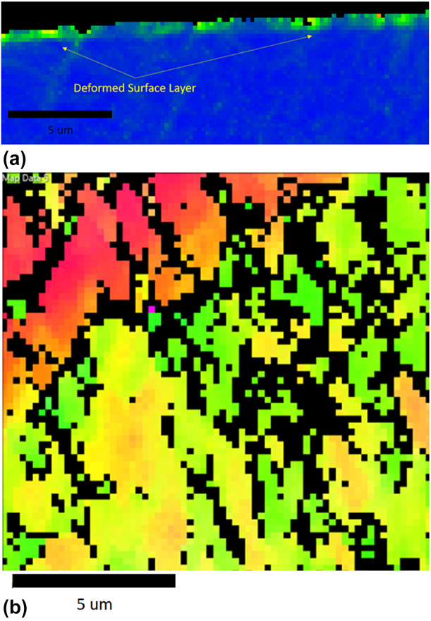
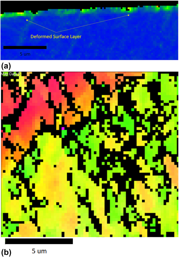
The calculated  $\overline {{\rho}}} _{{\rm{FD}}}}}$ variation with h in the as-polished condition is qualitatively consistent with the EBSD KAM map of the ion mill cross section of a deformed surface layer, as shown in Fig. 6(a). The deformation layer thickness indicated by the KAM map of the cross section is on the order of 1 µm and the effect of such a length scale is considered in a more quantitative fashion in Eq. (6). As expected, the KAM map of the mechanically polished surface plane shows extensive distortion [Fig. 6(b)]. Furthermore, the relationship between Fig. 6(a) and the interpretation in Fig. 5(d) was supported by examining the change in the extrinsic ISE as a function of heat treatment [Reference Soman, Herbert, Aifantis and Hackney13], where the observed reduction in H and reduction in KAM map distortion due to FD recovery during annealing were successfully analyzed by the Nes dislocation recovery model [Reference Nes42].
(a) KAM map of surface deformation cross section. (b) Plan view KAM map of as-polished surface.
Grain boundary indentation results
The modified Nix–Gao theory presented in Eqs. (2a) and (2b) was used to rationalize the mechanical polished grain interior indentation results in Fig. 5(d) by invoking a depth dependence in the FD density. The general approach introduced in Eq. (2) is now extended to the analysis of the extrinsic ISE of an isolated grain boundary. As reviewed above, nanoindentation studies of grain boundary mechanical behavior are certainly not new. Much attention has been devoted to the examination of how indentation just off the grain boundary in one grain must induce plasticity in the adjacent grain via slip transmission across the boundary. We have termed this remote indentation [Fig. 1(a)]. Such experiments can show P–h curve discontinuities proposed to occur at the point of slip transmission [Reference Aifantis, Deng, Shibata, Tsurekawa, Lejcek and Hackney18], corresponding to a local maximum in the H–h curve. These observations have been particularly prevalent in indentation of BCC metals and in particular Fe–C alloys, even with carbon content below the cementite solubility limit [Reference Britton, Randman and Wilkinson43]. However, the observation of local maximum in H due to remote indentation is not specific to BCC materials [Reference Voyiadjis and Yaghoobi6], although reports of discontinuity in P–h curves associated with such local maxima do appear to be specific to BCC materials. The focus of this paper is on what we have termed “‘local” indentation [Fig. 1(b)], where both adjacent grains undergo surface indentation at very small h.
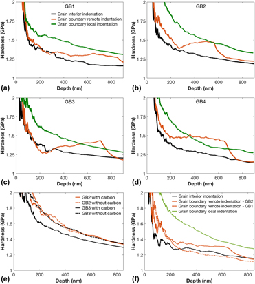
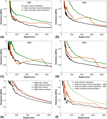
Figure 7 contrasts the H–h behavior for local and remote indentation in carbon-doped and H2:Ar heat-treated Fe. Figures 7(a)–7(d) contrasts local and remote indentation H–h behavior at 4 different grain boundaries in carbon-doped Fe. The difference between local and remote indentation is accentuated by the local maximum in H observed for the remote indentation. The extensive reverse ISE after h = 50 nm is only observed for the remote indentation geometry. Similar statements may also be made concerning the significant discontinuity in the H–h slope observed for the remote indentation H compared with the local indentation. It is also noted from further comparison of remote and local indentation H–h in Figs. 7(a)–7(d) that the H of the remote indentation curve falls below that of the local indentation H after the discontinuity and approaches the H of the grain interior. In remote indentation, the stress is “relieved” after yielding occurs at the grain boundary [Reference Aifantis, Deng, Shibata, Tsurekawa, Lejcek and Hackney18]. While for local indentation the high H is gradually reduced with deformation occurring simultaneously on both sides of the grain boundary. Collectively, these observations suggest two different hardening mechanisms are being probed by the two different indenter geometries (local versus remote). Although not commonly described in the literature, this conclusion concerning the role of indentation geometry at the grain boundary should not be surprising, as a distinction between grain boundary effects on yield point and grain boundary hardening post yield is well known [Reference Armstrong, Codd, Douthwaite and Petch44] for general, bulk deformation.
Representative hardness versus depth curves for from 4 different grain boundaries in a well annealed test specimen. (a)–(d) Show indentation results from the grain interior, the remote grain boundary indentation and the local grain boundary indentation for the carbon doped chemistry. (e) Comparison of local indentation for the same grain boundaries with and without carbon doping. (f) Comparison of local and remote grain boundary indentation with grain interior indentation with no carbon doping.

The remote indentation causes a progressive increase in equivalent stress at the grain boundary as indentation depth increases and the stress at the grain boundary eventually reaches an equivalent stress that causes plastic strain to initiate across the boundary. As such, the extrinsic ISE observed due to grain boundary remote indentation is measuring the grain boundary resistance to dislocations crossing the boundary, being emitted from the boundary and/or generated from a dislocation source across the boundary. This is effectively examining the plastic yield point at the grain boundary as envisioned by Hall [Reference Hall45] and Petch [Reference Petch46]. On the other hand, local indentation causes plastic deformation on both sides of the grain boundary early in the indentation process. As the local indentation will induce near simultaneous dislocation motion on non-coincident slip systems in the crystals on either side of the grain boundary, the result is expected [Reference Ashby3] to be incompatible shears within the indentation plastic volume. The strengthening observed for the local indentation of the grain boundary would, thus, be seen as probing the work hardening mechanism (post yield) of the grain boundary as originally envisioned by Ashby [Reference Ashby3]. The Ashby GND mechanism for accommodation of shear incompatibility across the grain boundary is certainly one of the more accepted mechanisms proposed for work hardening at the grain boundary. Hansen [Reference Hansen47] has utilized Ashby’s work on the local deformation at grain boundaries due to plastic strain incompatibility to analyze the experimental results and develop a grain boundary work hardening model with the same form as the Hall–Petch equation. This mechanism is still utilized in some computer simulations [Reference Evers, Parks, Brekelmans and Geers48] of polycrystalline plasticity as a solution to the Taylor–Sachs dichotomy. Also, these ideas continue to be developed in the more recent literature through self-consistent deformation models of polycrystalline materials [Reference Wierzbanowski, Baczmanski, Lipinski and Lodini49] and within the development of nonlocal constitutive models [Reference Ma and Hartmaier50].
Although not the focus of this paper, Fig. 7(e) compares local indentation H–h curves for the same grain boundaries in annealed H2:Ar specimens versus the carbon-doped specimens, indicating the H–h curves are statistically indistinguishable between the two. Figure 7(f) gives examples of remote and local indentation of H2:Ar heat-treated Fe. We note that some indentation curves do show the “hardening–softening” behavior reported for remote indentation of Al [Reference Voyiadjis and Yaghoobi6] but without the sharp discontinuity seen in Figs. 7(a)–7(d). Comparisons between Figs. 7(a)–7(d) and Figs. 7(e) and 7(f) are consistent with the concept that the observations of local indentation H–h are due to plastic strain geometry rather than grain boundary chemistry, while remote indentation results can be effected by grain boundary chemistry. Further support for the Ashby [Reference Ashby3] interpretation is also presented in Appendix B. However, a full analysis of this comparison of chemistry effects is not attempted in this paper and the focus is on the grain boundary hardness when plastic deformation is induced (approximately) simultaneously in both grains when the indenter tip is very close (“local”) to the grain boundary (0–0.5 μm) and the wedge of the indenter overlaps into the adjacent grain at small indentation depths.
The indentation behavior of an isolated grain boundary compared with grain interior behavior is shown in Figs. 5(a)–5(c). The increase in H and bilinear H 2 versus 1/h behavior specifically due to interaction with the grain boundary is isolated in Fig. 5(c). The increase in H with increase in  ${1 / {\sqrt h }}$ is suggestive of the Hall–Petch relationship. Historically, the three rationalizations for the classic Hall–Petch equation are pileup models [Reference Hall45, Reference Petch46]: (i) work hardening–based models [Reference Ashby3, Reference Hansen47] and (ii) grain boundary source models [Reference Li51]. Work hardening models correlate the increase in dislocation density due to the grain boundary to the flow stress. These work hardening models are particularly applicable to grain boundary effects on the flow curve at significant plastic strain and not generally considered applicable to grain boundary effects on yield strength. It is proposed that these work hardening models [Reference Ashby3, Reference Hansen47] will be most relevant to the local indentation geometry [Fig. 1(b)], given the initiation of plastic deformation on both sides of the grain boundary at low indentation depths. Following the approach in Eqs. (2a) and (2b), the effective depth dependence of a dislocation density that would correspond to the hardening response for indentation at a well-annealed grain boundary (GB2) may be calculated, as shown in Fig. 5(d). The calculated decrease in dislocation density with increasing h does reflect the extrinsic ISE at the grain boundary. We consider if such a size effect could be rationalized on the basis of the plastic strain gradient magnitude required at the boundary to accommodate local deformation incompatibility across the grain boundary [Reference Ashby3]. The scalar, “averaging” approach outlined by Nix and Gao [Reference Nix and Gao1] for the determination of the GND density for Berkovich indentation, is reduced to a single parameter (scaler measure) plastic displacement gradient (plastic strain), ∇u = tan(θ) = h/a, due to the slope of the indenter:surface contact. Interestingly, the number of GNDs is taken as a constant, h/b, with respect to the position under the indenter tip, although the authors point out that the strain gradient may not be uniform. This non-uniformity would certainly be consistent with Saint-Venant’s principle. For example, the Fourier series solutions to the biharmonic equations for the two-dimensional displacement compatibility conditions (plasticity or elasticity) have an exponential decay. It should also be noted that a grain boundary bisecting the indentation plastic volume will disrupt any semblance of spherical (axial) symmetry in the deformation field, even though the plastic volume itself may still be approximated as spherical. Extending the Nix–Gao [Reference Nix and Gao1] approach to a non-uniform strain gradient field with loss of axial symmetry, it is possible to consider the plastic displacement gradient to have an exponential form associated with the presence of the grain boundary as ∇u (gb) = γ exp(−y/λ), where γ is the maximum shear strain due to the “slope” of the plastic displacement caused by grain “overlap” [Reference Ashby3] related to plastic incompatibility, y is the direction perpendicular to the grain boundary, and λ is the decay length for this strain. The ∇u (gb) can be substituted for h/a in the original derivation [Reference Ashby3] for the GND density, with the average dislocation loop length taken as (πfh/2), giving Eq. (3a):
 $$\eqalign{\overline {{\rho _{{\rm{GND}}\left( {{\rm{gb}}} \right)}}} = {1 \over {{2 \over 3}\pi {{\left[ {fh} \right]}^3}}}\int_0^{fh} {{\gamma \over b}{{\rm{e}}^{{{ - y} / {\left( \lambda \right)}}}}{{\pi fh} \over 2}{\rm{d}}y} \cr= {{3\gamma \lambda } \over {4b{{\left( {fh} \right)}^2}}}\left( {1 - {{\rm{e}}^{{{ - fh} / \lambda }}}} \right)\quad .$$
Alternatively, Eq. (3a) can be rewritten as follows:
 $$\eqalign{\overline {{\rho _{{\rm{GND}}\left( {{\rm{gb}}} \right)}}} = {1 \over {{2 \over 3}\pi {{\left[ {fh} \right]}^3}}}\int_0^{fh} {{\gamma \over {bfh}}{{\rm{e}}^{{{ - y} / {\left( \lambda \right)}}}}{{\pi {{\left( {fh} \right)}^2}} \over 2}{\rm{d}}y} \cr= {{3\gamma \lambda } \over {4b{{\left( {fh} \right)}^2}}}\left( {1 - {{\rm{e}}^{{{ - fh} / \lambda }}}} \right)\quad ,$$
where γ/(bfh) is the ρGND(gb) at the grain boundary (Ashby [Reference Ashby3]) and π(fh)2/2 is an approximation for the small circle area (disc) that the dislocation “lines” intersect. Equations (3a) and (3b) utilize the same approach as the original Nix–Gao [Reference Nix and Gao1] treatment, as modified by Durst et al. [Reference Durst, Backes and Goken4], that the plastic deformation gradient imposed by the geometry of the indenter results in GNDs spread over some fraction of the indentation plastic volume. The Nix–Gao–Durst approach considers a volume of integration with radius [fh/tan(θ)]. Analogous to this idea is that the excess dislocations produced by the deformation at the grain boundary is spread over a fraction of the indentation plastic volume, (fh), which is much less than the grain size as the grain size here is >1 mm [Fig. 2(a)]. Further justification for using (fh) as a proxy for grain size comes from the work of Meakin and Petch [Reference Meakin and Petch52, Reference Kato53], who considered that the dislocation slip length was some fraction of the grain diameter and thus the dislocation density is inversely proportional to the grain size. This was later confirmed by the works of Conrad et al. [Reference Conrad, Feuerstein and Rice54, Reference Conrad55]. The ISE can be interpreted in a similar manner as the grain size effect [Reference Meakin and Petch52] in that the dislocation density due to indentation appears to have an inverse relationship with the contact radius. For indentation local to the grain boundary [Fig. 1(b)], the argument analogous to Meakin and Petch is that the slip length of the dislocation due to plastic strain at the grain boundary is some fraction of the indentation plastic zone diameter.
Equation (3b) can be correlated with the idea of an extrinsic ISE by noting the h dependence of the  $\overline {{\rho _{{\rm{GND}}\left( {{\rm{gb}}} \right)}}}$. If the decay length, λ, is proportional to h, then the “standard” 1/h dependence for H 2 is recovered. Utilizing the same approach as in Eq. (2a) leads to Eq. (4a), with
 $h_{{\rm{gb}}}^{\rm{*}}$ as the characteristic length scale for the extrinsic ISE due to the grain boundary [Eq. (4b)].
 $${H^2} = {H_0}^2\left( {1 + {{{h^*}} \over {h{f^3}}} + {{h_{{\rm{gb}}}^{\rm{*}}} \over {h{f^3}}}} \right)\quad ,$$
where from Eq. (3)
 $$h_{{\rm{gb}}}^{\rm{*}} = {1 \over {{\rho _{{\rm{SSD}}}}}}{{3\gamma \lambda f} \over {4bh}}\left( {1 - {{\rm{e}}^{ - {{fh} \over \lambda }}}} \right)\quad ,$$
such that, analogous to Eqs. (1a)–(1d),
 $${H_0}^2{{h_{{\rm{gb}}}^{\rm{*}}} \over {h{f^3}}} = {\left( {3\sqrt 3 \alpha Gb} \right)^2}\overline {{\rho _{{\rm{GND}}\left( {{\rm{gb}}} \right)}}} \quad .$$
It is noted that if λ in Eq. (4b) is proportional to h, then a constant  $h_{{\rm{gb}}}^{\rm{*}}$ is recovered. The characteristic length scales,
 ${{{h^*}} \over {{f^3}}}$ and
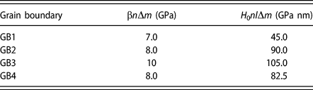
 ${{h_{{\rm{gb}}}^{\rm{*}}} \over {{f^3}}}$, can also be determined by matching Eq. (4) to the experimental H 2 versus 1/h curves for the data corresponding to the grain surfaces, GB1, GB2, GB3, and GB4 (Table I), as shown in Fig. 5(c). The H 0 values (H for “infinite” indentation depth) can be determined by extrapolating the H 2 versus 1/h to 1/h = 0. A curve fit the grain boundary H 2 versus 1/h curve over the indentation depths of 500–1000 nm gives H 0 = 1.05 GPa (R 2 = 0.97). However, the substantial bilinearity of the grain boundary H 2 versus 1/h curve produces a larger H 0 value when the grain boundary H 2 at indentation depths of 200–500 nm are extrapolated to 1/h = 0. Thus, we limit the consideration of the grain boundary H 2 curve to indentation depths greater than 500 nm. With this approach, the h*/f 3 is determined using the slope of the grain interior H 2 versus 1/h plot and is reported in Table I. Having determined H 0 and h*/f 3 from the grain interior data of the harder adjacent grain, Eq. (4a) can now be fit to the extrinsic component of the grain boundary H 2 versus 1/h plot, where
 ${{h_{{\rm{gb}}}^*} / {{f^3}}}$ is the fitting parameter. If the Hall–Petch coefficient, k, is specifically defined as a multiplier relating local dislocation density to the inverse square root of grain size [Reference Ashby3, Reference Hansen47, Reference Conrad55, Reference Kocks56] and fh as a proxy for grain size, then Eq. (4c) gives the relation:
 $${k \over {\sqrt f }} = {{{H_0}} \over 3}\sqrt {{{h_{{\rm{gb}}}^*} / {{f^3}}}} {1 \over {\sqrt f }}\quad ,$$
where the factor 1/3 in Eq. (5) relates the grain boundary H as three times the uniaxial stress at the same strain (Tabor’s relationship). The curve fit results for f = 1 are shown in Table I and show values for k of the same order as that determined by bulk mechanical testing of low carbon and interstitial free steels (k = 0.11 MPa m1/2) [Reference Takeda, Nakada, Tsuchiyama and Takaki57]. Alternatively, f may be calculated from Eq. (5) using the graphically determined values of H 0 and  ${{h_{{\rm{gb}}}^{\rm{*}}} / {{f^3}}}$ in Table I together with the experimental result [Reference Nes42] of k = 0.1 MPa m1/2, giving the range f ∼ 2.0 to 3.2. This range in f does bracket the value of the contact radius to indentation depth ratio for a cone geometry with included angle of 70°, a/h = tan(θ)−1 = 2.74, suggesting that the grain size proxy is the same order as the contact radius. As support for the utilization of Eq. (5), it should be noted that Rester et al. [Reference Rester, Motz and Pippan14] have introduced the concept that GNDs caused by the indentation geometry will form cell walls or subgrains due to dynamic recrystallization and it is these “grain boundaries” under the indenter contact area that result in the intrinsic ISE. Although Rester et al. [Reference Rester, Motz and Pippan14] consider the grain boundary strengthening is due to dynamic recrystallization as a “substitution” for the GND strengthening, the general idea of grain boundary strengthening due to a preexisting grain boundary under the indentation contact area is a natural extension of their analysis.
Analysis of intrinsic and extrinsic ISE related to specific grain boundaries.

It is of interest to extend the concepts leading to Eq. (3b) to the extrinsic, one- and two-dimensional dislocation distributions described in Fig. 5, determined from the procedure described in Soman et al. [Reference Soman, Herbert, Aifantis and Hackney13]. In contrast to Eqs. (3b), (2a), and (2b) do not interrogate the dimensionality of the preexisting dislocation distributions, although the results from Eqs. (2a) and (2b) should be self-consistent with such an approach if there is any inherent validity. One issue is that the approximation of indentation strain spherical symmetry is broken when considering the dimensionality of the preexisting defect distributions studied here. It is thus suggested that dislocation density averaging is most straightforward using the Cartesian coordinate system such that
 $$\eqalign{\bar{\rho } = {{3{\rho _0}} \over {2\pi {{\left( {fh} \right)}^3}}}\int_0^{fh} {\int_0^{fh} {\int_0^{fh} {S\exp \left( { - {x \over {{\lambda _x}}}} \right)\exp \left( { - {y \over {{\lambda _y}}}} \right)}}}\cr\exp \left( { - {z \over {{\lambda _z}}}} \right){\rm{d}}x{\rm{d}}y{\rm{d}}z} } } \quad ,$$
where ρ0 is the maximum dislocation density in the vicinity of the surface origin (x = 0, y = 0, z = 0). The value S = 8π/3 is determined, so ρ0 is returned if all the direction-dependent decay lengths, λi, go to infinity, which would be equivalent to uniform deformation. The values of the decay lengths λi thus set the dimensional dependence of the extrinsic ISE. Specifically, for the one-dimensional dislocation density gradient (surface layer deformation, Fig. 6), only the direction normal to the surface will have a finite decay length as in Eq. (7a).
 $$\eqalignb{{{3{\rho _0}} \over {2\pi {{\left( {fh} \right)}^3}}}\int_0^{fh} {\int_0^{fh} {\int_0^{fh} {S\exp \left( { - {x \over {{\lambda _x}}}} \right){\rm{d}}x{\rm{d}}y{\rm{d}}z}}} \cr= {\rho _0}{{4{\lambda _x}\left( {1 - {{\rm{e}}^{ - {{fh} \over \lambda }}}} \right)} \over {fh}}} } } \quad .$$
For the row of closely spaced shallow indentations, the preexisting distribution from the overlapping indentations is taken to have cylindrical symmetry extending along the z-axis. Thus, the surface normal direction (x) and the orthogonal direction (y) will have decay lengths that are finite and equal (λx = λy) [Eq. (7b)].
 $$\eqalignb{{{3{\rho _0}} \over {2\pi {{\left( {fh} \right)}^3}}}\int_0^{fh} {\int_0^{fh} {\int_0^{fh} {S\exp \left( { - {x \over {{\lambda _x}}}} \right)\exp \left( { - {y \over {{\lambda _y}}}} \right){\rm{d}}x{\rm{d}}y{\rm{d}}z}}} \cr= {\rho _0}{{16{\lambda ^2}\sinh {{\left( {{h / {\left( {2\lambda } \right)}}} \right)}^2}} \over {{{\left( {fh} \right)}^2}}}{{\rm{e}}^{ - {{fh} \over \lambda }}}} } } \quad .$$
A comparison of Eqs. (7a) and (7b) with the dislocation density results from Eqs. (2a) and (2b) is shown in Fig. 5(d), with λ/f = 193 nm and ρ0 = 7 × 10¹⁵ m−2 for the surface deformation and λ/f = 125 nm and ρ0 = 2.4 × 10¹⁶ m−2 for the indentation row deformation. This comparison shows that the proposed approach is consistent with observed 1/h dependence for the one-dimensional (surface) deformation gradient versus the observed 1/h 2 dependence for the two-dimensional (indentation row) deformation gradient. It should be noted that although GNDs may be present within these fixed distributions related to prior deformation, these are not specific to the indentation geometry in the present experiment. In any case, the excellent fit for Eqs. (6) and (7) in Fig. 5(d) suggests the extrinsic ISE for these preexisting defects is apparently controlled by their inherent distribution and dimensionality prior to the indentation process.
When considering the grain boundary indentation using the approach leading to Eqs. (6) and (7), the dislocation density distribution due to the presence of the grain is taken as decaying primarily perpendicular to the grain boundary plane (in one dimension) and is, thus, the same form (geometry) as for the surface deformation [Eq. (7a)], but with a decay length proportional to the grain size, or in our case, h. This is consistent with the Ashby [Reference Ashby3] theory of grain boundary GNDs. Again following Ashby [Reference Ashby3], the average GND density at the grain boundary is considered inversely proportional to h in Eq. (3a) with dislocation loop length (πfh). Using a proportionality constant, n, such that λ = (fh)/n, then Eq. (6) can be rewritten for the grain boundary case as follows:
 $$\eqalignb{\left[ {{{\pi \gamma } \over {bfh}}} \right]{3 \over {2\pi {{\left( {fh} \right)}^3}}}\int_0^{fh} {\int_0^{fh} {\int_0^{fh} {S\exp \left( { - {y \over \lambda }} \right){\rm{d}}x{\rm{d}}y{\rm{d}}z}}} \cr= {{4\pi \gamma } \over {bfh}}{{\left( {1 - {{\rm{e}}^{ - n}}} \right)} \over n}} } } \quad .$$
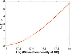
As in the case for the one- and two-dimensional extrinsic deformation gradients, the integral equation solution [Eq. (8) with  ${{4\pi \gamma } / {bf}}\left( {{{\left( {1 - {{\rm{e}}^{ - n}}} \right)} \over n}} \right) = 4.5 \times {10^8}\;{{\rm{m}}^{ - 1}}$] well represents the dislocation density distributions determined from the extrinsic ISE at one of the grain boundaries (GB2) in Fig. 5(d). The implications of the results for Eqs. (5) and (8) are considered further in Appendix B. In the Analysis section, a continuum SGP approach with considerably greater mathematical structure, relative to Eq. (8), is considered.
Analysis: continuum SGP formulation and the SGP boundary condition related to the Ashby model
The analysis developed here is not meant to be predictive but rather to be interpretive in exposing the physics of the additive effects of intrinsic and extrinsic ISE. As such, an approximate analytical approach is pursued using a two-dimensional argument with prescribed displacements (strains) within the context of a continuum SGP theory. The purpose of this exercise is to connect Eq. (4a) to more specific considerations of the spatial dependence of plastic strain. A simple physical description of the Ashby [Reference Ashby3] proposal will be utilized to develop an appropriate boundary condition for the linear continuum model in the case of anisotropic plastic shape change for the adjacent grains, designated 1 and 2. The approach centers around the relation between the plastic strain, εp, along a specific loading direction (x) and the shear strain, γ, that occurs on specific crystallographic planes. For a scaler argument with single slip, the normal plastic strain component is given in terms of the shear and the product of the slip system direction cosines (m) as follows:
 $${\varepsilon _{\rm{p}}} = \gamma \cos \left( \theta \right)\cos \left( \emptyset \right) = \gamma m\quad ,$$
where m is also known as the Schmid factor. Alternatively, m = dεp(x)/dγ, as defined by Taylor [Reference Taylor19]. For indentation local to the grain boundary, it is expected that the plastic displacement at the surface will be equivalent in both grains at the grain boundary. But if m for grain 1 is different from m for grain 2, then γ1 will be different from γ2 or,
 $${\gamma _1} - {\gamma _2} = {\varepsilon _{\rm{p}}}{{{m_1} - {m_2}} \over {{m_1}{m_2}}}\quad .$$
Ashby uses the difference in plastic shear strain across the grain boundary to determine the additional plastic displacement at the grain boundary, u gb, required for plastic compatibility. This plastic displacement scales with the grain radius, D, as
 $${u_{{\rm{gb}}}} = {\varepsilon _{\rm{p}}}D{{{m_1} - {m_2}} \over {{m_1}{m_2}}}\quad .$$
This plastic strain, u gb/D, is in addition to the imposed plastic strain, εp, which according to Taylor [Reference Taylor19] would correspond to the operation of additional slip systems to allow for strain compatibility across the grain boundary. Ashby further implies that the excess plastic strain will decay with position away from the grain boundary by noting the development of ρGND at the grain boundary as
 $${\rho _{{\rm{GND}}}} = {{{u_{{\rm{gb}}}}} \over b}{1 \over {DL}} = {{{\varepsilon _{\rm{p}}}} \over {bL}}\Delta m\quad ,$$
where
 $$\Delta m = {{{m_1} - {m_2}} \over {{m_1}{m_2}}}\quad ,$$
where the width L is the distance from the grain boundary that contains the bulk of the GNDs and may be considered as the decay length of the excess plastic strain. This length scale, L, may be considered equivalent to that described in Evers et al. [Reference Evers, Parks, Brekelmans and Geers48] for the grain boundary deformation layer thickness required for compatibility due to anisotropic plastic deformation. Evers et al. [Reference Evers, Parks, Brekelmans and Geers48] considered L to be proportional (but not equal) to the grain radius, while Ashby [Reference Ashby3] took this width to be equivalent to the grain diameter. Although the analysis to be developed here is not accurate enough to give a conclusive argument for either the Ashby [Reference Ashby3] or Evers [Reference Evers, Parks, Brekelmans and Geers48] approach to the decay length for the excess plastic strain, it is to be implicitly included.
The generally accepted relationship between the density of GNDs and the plastic strain gradient, apparently first proposed by Ashby [Reference Ashby3], is as follows:
 $${\rho _{{\rm{GND}}}} = {1 \over b}\left( {{{\rm{d}} \over {{\rm{d}}y}}{\varepsilon _{\rm{p}}}} \right)\quad .$$
Using Eq. (14) with Eq. (12) gives
 $${{{\varepsilon _{\rm{p}}}} \over L}\Delta m = \left( {{{\rm{d}} \over {{\rm{d}}y}}{\varepsilon _{\rm{p}}}} \right)\quad ,$$
which is used as a boundary condition at the grain boundary for the development of the continuum plasticity analysis to follow. The rhs of Eq. (15) can be interpreted as the increase in plastic strain due to a non-zero Δm, which decays over the length, L, as defined by the spatial derivative on the lhs of Eq. (15). The occurrence of an excess in plastic strain beyond the imposed plastic strain, Eq. (11), together with a gradient in plastic strain does suggest a peak in a scaler measure of plastic strain magnitude at the grain boundary. For dislocation density proportional to the square of the strain and proportional to the strain gradient, a significant increase in dislocation density is then expected at the grain boundary and the experimental results of Vachhani et al. [Reference Vachhani, Doherty and Kalidindi20] are seen to be particularly relevant.
The formulation for the SGP continuum analysis that can be adapted to the linear analysis pursued here is described in a recent publication by Wei et al. [Reference Wei, Konstantinidis, Qi and Aifantis58].
 $$\sigma = \beta \left( {\overline {{\varepsilon _{\rm{p}}}} + {l_1}{{\left[ {\vec{\nabla }\overline {{\varepsilon _{\rm{p}}}} \Delta \vec{\nabla }\overline {{\varepsilon _{\rm{p}}}} } \right]}^{\rm{q}}} + {l_2}{\nabla ^2}\overline {{\varepsilon _{\rm{p}}}} } \right)\quad ,$$
where β is the hardening modulus. For the analysis here, the characteristic length l 2 = 0 and the exponent = 1/2, as represented by Eqs. (A.1) and (A.3) in Appendix A. The equivalent stress, σ, is a function of the equivalent plastic strain measures, 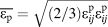 $\overline {{\varepsilon _{\rm{p}}}} = \sqrt {\left( {{2 / 3}} \right)\varepsilon _{ij}^{\rm{p}}\varepsilon _{ij}^{\rm{p}}}$ and the magnitude of the gradient squared
 $\left( {\vec{\nabla }\overline {{\varepsilon _{\rm{p}}}} \Delta \vec{\nabla }\overline {{\varepsilon _{\rm{p}}}} } \right)$ as utilized in Eq. (16), where
 $\varepsilon _{ij}^{\rm{p}}$ is the plastic strain tensor. The details of the solution to Eq. (16) are given in Appendix C.
The stress contribution from the grain boundary to the averaged equivalent stress at the surface and the extrinsic ISE is found to have the form:
 $${\left[ {\overline {{\sigma _{\left( {{\rm{gb}}} \right)}}} {|_{x = {\pi \!\left/{\vphantom{\pi {\left( {2\omega } \right)}}}\right.{\left( {2\omega } \right)}}}}} \right]_{{\rm{extrinsic}}}} = \left( {{{0.12n{H_0}{l_1}\Delta m} \over h}} \right) + 0.02n\beta \Delta m\quad .$$
Drawing from the concepts leading to Eq. (A.8) the total stress from the addition of the intrinsic and extrinsic components of the deformation is then used to estimate H:
 $$H = {\left[ {{H_0}\left( {1 + {{{h^*}} \over {2{f^3}h}}} \right)} \right]_{{\rm{intrinsic}}}} + {\left[ {\overline {{\sigma _{\left( {{\rm{gb}}} \right)}}} {|_{x = {\pi \!\left/{\vphantom{\pi {\left( {2\omega } \right)}}}\right.{\left( {2\omega } \right)}}}}} \right]_{{\rm{extrinsic}}}}\quad .$$
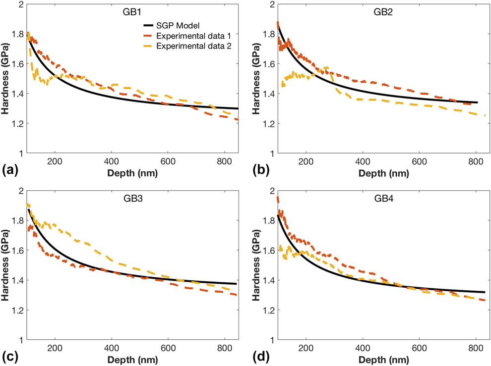
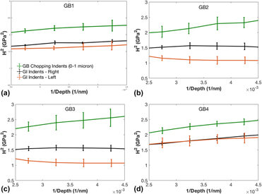
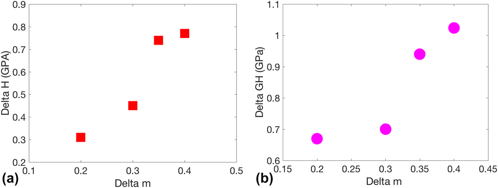
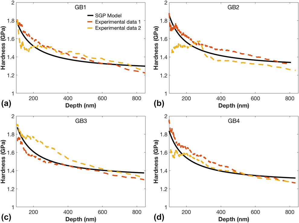
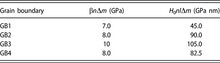
Although the approach leading to Eq. (18) is linear, two dimensional and limited to a single Fourier coefficient, it is possible to still have a reasonable comparison with the experimental results obtained from local grain boundary indentation, as presented in Figs. 5 and 7. This comparison between Eq. (18) and the local indentation experimental results for 4 different grain boundaries is shown in Fig. 8 with the two independent fit parameters detailed in Table II. These two fit terms are multiplicative products of parameters but still may be judged as the same order as that determined in Eq. (4) (Table I) with the limiting case for the values of Δm examined in Appendix B.
The comparison of the continuum SGP model Eq. (18) with the experimental results from local indentation on the 4 grain boundaries (a–d). Two experimental curves (dashed) from each boundary representing the variance of the behavior are presented. The solid curve is the fit from Eq. (18).
The extrinsic component of Eq. (18) can be compared with  ${{{H_0}h_{{\rm{gb}}}^{\rm{*}}} / {{f^3}}}$ in Eq. (4) and Eq. (A.9) as follows:
 $${H_0}{{h_{{\rm{gb}}}^*} \over {2{f^3}}} = \left( {0.12{H_0}{l_1} + 0.02\beta h} \right)n\Delta m\quad .$$
The nonequivalence of  $h_{{\rm{gb}}}^*$ and l in Eq. (19), as discussed in Appendix A, can be resolved by taking
 ${H_0} = \beta b\sqrt {\overline {{\rho _{{\rm{SSD}}}}} }$ and noting from Appendix A that
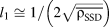 ${l_1} \cong {1 / {\left( {2\sqrt {\overline {{\rho _{{\rm{SSD}}}}} } } \right)}}$. Equation (19) provides the insight that the characteristic length,
 ${{h_{{\rm{gb}}}^{\rm{*}}} / {{f^3}}}$, can be described as a function of h. The possibility of strain dependence for the characteristic length in gradient theories has been considered previously [Reference Wei, Konstantinidis, Qi and Aifantis58, Reference Evans and Hutchinson59, Reference Zhang and Aifantis60], but a specific discussion of
 ${{h_{{\rm{gb}}}^{\rm{*}}} / {{f^3}}}$ dependence on h has only been previously described in the work of Feng at al. [Reference Feng and Nix61], which considers the volume correction factor, f, as inversely proportional to h. This conclusion [Reference Feng and Nix61] is consistent with the finding in Eq. (19).
The parameter, (H 0l 1)nΔm, on the right-hand side of Eq. (19) has special significance as a description of (energy dissipation)/area, or mechanically induced interface energy, due to deformation at the grain boundary. This term describes the deformation energy cost for the formation of GNDs seen in Eqs. (14) and (15). The physical basis of how the grain boundary GNDs contribute to the strengthening can be illustrated using Eqs. (A.6) and (A.7) as follows:
 $$\sigma _{{\rm{gb}}}^{{\rm{GND}}} = \beta b\left( {{\rho _{{\rm{GND}}}}{l_1}} \right) = \beta b\left( {{{{H_0}} \over {\beta bh}}{l_1}} \right)n\Delta m\quad .$$
Rewriting Eq. (20a) as
 $$\sigma _{{\rm{gb}}}^{{\rm{GND}}}h = \left( {{H_0}{l_1}} \right)n\Delta m\quad ,$$
where the rhs of Eq. (20b) is constant within the error of the curve fitting in Fig. 8, indicating the same for the lhs of Eq. (20b). The values for [(H 0l 1)nΔm] are listed in Table II and may be interpreted through the work of Aifantis and Willis [Reference Aifantis and Willis27, Reference Aifantis and Willis28] who introduced (phenomenologically) a specific interface parameter that characterizes the grain boundary strength and is termed a, γ, or ξ with units of Pa/m2 or N/m. In a recent study [Reference Aifantis, Deng, Shibata, Tsurekawa, Lejcek and Hackney18], the value of ξ was deduced by directly relating remote nanoindentation [Fig. 1(a)] data for grain boundaries in Fe–3wt% Si. The values found for the Fe–3wt% Si ξ were 291–400 N/m, depending on the grain boundary type. Although the same order, as described in Table II, a one to one comparison is difficult because the difference in alloy content and indentation geometry.
It should be noted that in interfacial gradient plasticity the interface parameter (ξ) is introduced within a mechanical interface energy Φ, which is a function of the plastic strain on the GB. Letting ξ = (H 0l 1)nΔm would then imply that
 $$\Phi = {\beta \over 2}b\left( {{{\left( {{{{H_0}} \over \beta }} \right)}^2}{{{l_1}} \over b}} \right)n\Delta m\quad ,$$
where H 0/β is the indentation plastic strain for very large h. Such a quadratic dependence of Φ on the square of the plastic strain was postulated for a grain boundary that begins deforming simultaneously as the adjacent grain [Reference Aifantis and Willis62], which is in fact the case in the present indentation experiments. Reports on these types of boundary energy dissipation terms have increased in development and application since the inception in a series of papers by Aifantis and Willis [Reference Aifantis and Willis62]. However, this appears to be the first instance, where a boundary dissipation term has been considered for the Ashby grain boundary deformation mechanism.
The comparison of Eqs. (18) and (19) with Eqs. (3), (4), and (8) allows us to close the loop on the arguments developed herein. The exponential dependence of plastic strain and dislocation density utilized in these equations is seen to be consistent with a solution based on the Marguerre function in Eq. (C.3a). Similarly, to determine the average equivalent stress under the indenter, the exponential decay of flow stress from the grain boundary position at y = 0 must be integrated, analogous to integrating the spatial variation (exponential decay) of dislocation density in Eq. (8). Finally, the solution to Eq. (16) in Appendix C gives the plastic strain gradient at the grain boundary, proportional to the GND density, as
 $$\left| {\nabla \overline {{\varepsilon _{\rm{p}}}} } \right|{|_{y = 0}} \propto \left| {{{{H_0}\Delta m} \over {\beta L}}} \right|\quad ,$$
where it is reiterated that L can be considered proportional to h. Note that  ${H_0} = \beta \overline {{\varepsilon _{\rm{p}}}} {|_{\Delta m = 0}}$ and then Eq. (21) is consistent with Eqs. (3), (4), (8), (12), and (15). The continuum SGP solution [Eq. (18)] does suggest that both the plastic strain and the strain gradient magnitude will increase at the grain boundary, indicating the grain boundary will be “harder” than the adjacent material for β > 0. The local increase in plastic strain and plastic strain gradient magnitude, and thus dislocation density, at the grain boundary is also explicit in the integral kernel showing exponential decay of dislocation density in Eqs. (3) and (8). However, the physical origin is only explicit in the continuum SGP solution and may be identified as the boundary condition of Eq. (C.7b). The “uniform” imposed plastic displacement at the surface–grain boundary intersection in Eq. (C.7b) is reminiscent of the parallel loading for polycrystalline materials, as originally envisioned by Taylor [Reference Taylor19], while the spatial variation in plastic strain is suggestive of the polycrystalline deformation process conceptualized by Sachs [Reference Sachs63]. To support the result of spatial variation in stress and plastic strain (dislocation density), it is recalled that the experimental work of Vachhani [Reference Vachhani, Doherty and Kalidindi20] does show local grain boundary hardening occurs in deformed Al (as measured post yield), and this is consistent with the concept that the total dislocation density is increased there.
Conclusions
The extrinsic ISE for preexisting, one- and two-dimensional deformation gradients is rationalized through an extension of the Nix–Gao [Reference Nix and Gao1] integral averaging approach of dislocation densities to allow for explicit consideration of the dimensionality of the dislocation density distribution. This approach can be applied to the extrinsic ISE observed for local indentation of grain boundaries in Fe and carbon-doped Fe. Even though the extrinsic ISE due to the grain boundary can be modeled as a one-dimensional deformation gradient using this approach, the underlying mechanism causing the increase in grain boundary hardening could not be explicitly addressed. However, utilizing the Ashby [Reference Ashby3] theory of grain boundary GND, a simple application of a continuum SGP model [Reference Wei, Konstantinidis, Qi and Aifantis58] is found to be qualitatively consistent with the integral kernel constructed for the dislocation distribution in the vicinity of a deformed grain boundary. Particularly, it was possible to interpret the interface parameter ξ (which has been introduced within interfacial gradient plasticity) as being equal to the product of the hardness of the GND free grain, the Δm, and the internal length. The simple continuum SGP analysis employed here also reveals the structure of the plasticity distribution at the grain boundary, suggesting that both the plastic strain and plastic strain gradient increase there. This continuum SGP result is consistent with previously published, independent experimental [Reference Vachhani, Doherty and Kalidindi20] and theoretical [Reference Evers, Parks, Brekelmans and Geers48] analyses.
Acknowledgment
This work was supported by Office of Basic Energy Sciences within the Department of Energy (DOE) Award Number: DE-SC0016314 and DE-SC0017715.
Appendix A. Linearization of the Taylor Hardening flow stress relation.
This paper focusses on the correlation of ISE with indentation depth-dependent dislocation density through the Taylor hardening flow rule. Ashby [Reference Ashby3] has suggested that the plastic (in)compatibility at the grain boundary may be correlated with an increase in density of GNDs there, then leading to an increase in hardening due to the Taylor hardening mechanism [Reference Samuels38]. GNDs were correlated to the gradient in plastic strain by Ashby in 1970 [Reference Ashby3] and as such was part of the origination of SGP theories, which proliferate the literature 50 years later. The continuum models of SGP do have a linearized forms that have been used successfully to develop analytical approaches to aid in the physical interpretation of deformation phenomenon [Reference Wierzbanowski, Baczmanski, Lipinski and Lodini49]. Given the focus on the Taylor hardening mechanism in this work, it is of interest and a necessity to relate the mechanistic Taylor dislocation hardening relation to this linear, relatively transparent continuum SGP analysis. The first step in such an analysis is to examine under what conditions the Taylor strengthening equation, upon which Eqs. (1)–(8) are based, can be consistent with the linear continuum SGP flow rule. This particular issue relating Taylor flow theory with a continuum SGP model has been discussed previously [Reference Mokios and Aifantis64], although using an approach different from that pursued here. We attempt here to relate an SGP linear flow stress model to the Taylor flow rule by relating the plastic strain and plastic strain gradient to the dislocation density as follows:
 $$\sigma \left( x \right) = \beta \left[ {{\varepsilon _{\rm{p}}} + l\left( {{{\rm{d}} \over {{\rm{d}}x}}{\varepsilon _{\rm{p}}}} \right)} \right] \cong \beta b\sqrt {{\rho _{{\rm{SSD}}}}\left( x \right) + {\rho _{{\rm{GND}}}}\left( x \right)} \quad ,$$
where σ(x) is a position-dependent flow stress, β is the hardening modulus, εp is the plastic strain, l is a characteristic length, and x is the position variable. Equation (A.1) is rewritten by defining  $\overline {{\rho _{{\rm{SSD}}}}}$ as the volume averaged SSD dislocation density and ΔSSD(x) as the variation in the SSD dislocation density about the average:
 $$\sigma \left( x \right) = \beta b\sqrt {\overline {{\rho _{{\rm{SSD}}}}} + {\Delta _{{\rm{SSD}}}}\left( x \right) + {\rho _{{\rm{GND}}}}\left( x \right)} \quad .$$
Relating Eq. (A.2) to indentation,  $\overline {{\rho _{{\rm{SSD}}}}}$ is the average dislocation density for indentation in the grain interior and is not a function of position(x). A pyramid, wedge, or spherical tip would develop position-dependent dislocation densities due to the indenter geometry [Reference Nix and Gao1]. The presence of a grain boundary in the indentation volume is also considered here to introduce spatial variations in dislocation density. Equation (A.2) is approximated to Eq. (A.3) through the sequential Taylor series on the smaller terms, ΔSSD(x) and ρGND(x), and compared with the linear SGP flow stress rule in Eq. (A.1)
 $$\eqalign{\beta \left[ {{\varepsilon _{\rm{p}}} + l\left( {{{\rm{d}} \over {{\rm{d}}x}}{\varepsilon _{\rm{p}}}} \right)} \right] \cr= \beta b\left\{ {\sqrt {\overline {{\rho _{{\rm{SSD}}}}} } + {1 \over {2\sqrt {\overline {{\rho _{{\rm{SSD}}}}} } }}\left[ {{\Delta _{{\rm{SSD}}}}\left( x \right) + {\rho _{{\rm{GND}}}}\left( x \right)} \right]} \right\}\quad .$$
The comparison of the lhs and rhs of Eq. (A.3) is carried out by noting the Orowan equation:
 $${\varepsilon _{\rm{p}}} = \rho bX = \rho b{1 \over {\sqrt \rho }}\sim \left[ {\sqrt {\overline {{\rho _{{\rm{SSD}}}}} } + {{{\Delta _{{\rm{SSD}}}}\left( x \right)} \over {2\sqrt {\overline {{\rho _{{\rm{SSD}}}}} } }}} \right]\quad ,$$
where X is the slip length, which can be taken as the dislocation spacing. To correlate the plastic strain as defined in Eq. (A.4) with Eq. (A.1), it is necessary to take the derivative of the plastic strain. Given Eq. (A.4) and the well-known relation [Reference Ashby3],
 $${{\rm{d}} \over {{\rm{d}}x}}{\varepsilon _{\rm{p}}} = b{\rho _{{\rm{GND}}}} \sim \,b{{\rm{d}} \over {{\rm{d}}x}}\left[ {{{{\Delta _{{\rm{SSD}}}}\left( x \right)} \over {2\sqrt {\overline {{\rho _{{\rm{SSD}}}}} } }}} \right]\quad .$$
Then, it is possible to rewrite Eq. (A.1) to first order in small terms using Eqs. (A.4) and (A.5):
 $$\eqalign{\sigma \left( x \right) = \beta \cdot \left[ {{\varepsilon _{{\rm{p}}\left( x \right)}} + l\left( {{{\rm{d}} \over {{\rm{d}}x}}{\varepsilon _{{\rm{p}}\left( x \right)}}} \right)} \right]\cr\sim\beta b\left[ {\sqrt {\overline {{\rho _{{\rm{SSD}}}}} } + {{{\Delta _{{\rm{SSD}}}}\left( x \right)} \over {2\sqrt {\overline {{\rho _{{\rm{SSD}}}}} } }} + l{\rho _{{\rm{GND}}}}\left( x \right)} \right]\quad ,$$
where l is defined through Eqs. (A.3) and (A.6) as 1/2 the average dislocation spacing:
 $$l = {1 \over {2\sqrt {\overline {{\rho _{{\rm{SSD}}}}} } }}\quad .$$
The error involved in the analysis leading to Eqs. (A.6) and (A.7) may be determined by Eq. (A.8). It may be seen in Fig. A1 that the error is less than 6% when the averaged dislocation density  $\overline {{\rho _{{\rm{SSD}}}}} = \overline {{\rho _{{\rm{GND}}}}} = {10^{18}}\;{{\rm{m}}^2}$. This sacrifice in precision is required for a transparent analysis of the observed phenomena. As support for the overall result developed in Eqs. (A.1)–(A.7), the definition of the length scale in Eq. (A.7) is seen to be consistent with the conclusions of Evans and Hutchinson [Reference Evans and Hutchinson59] obtained by attempting to relate the plastic dissipation term for the linear flow rule to the Taylor hardening expression. Physically, Eqs. (A.6) and (A.7) is describing the contribution that the “extra” dislocation from the spatial variation in plastic strain will make toward the total dislocation hardening, so that for small l, the contribution for a given deformation gradient to the total hardening will be limited. This is a direct consequence of the additive formulation for the different dislocation densities in Eq. (A.2). However, this physical description does not take into account that the deformation gradient magnitude may increase with a decrease in the slip length, l, depending on the boundary conditions.
 $$\% {\rm{Error}} = \left( {1 - {{\sqrt {\overline {{\rho _{{\rm{SSD}}}}} + \overline {{\rho _{{\rm{GND}}}}} } } \over {\sqrt {\overline {{\rho _{{\rm{SSD}}}}} } + {{\overline {{\rho _{{\rm{GND}}}}} } \over {2\sqrt {\overline {{\rho _{{\rm{SSD}}}}} } }}}}} \right)100\quad .$$
Percent error in Eq. (A.6) when compared to Eq. (A.1). The error is less than 1% when ρgb = 0.1 ρA and is ∼6% at ρgb = ρA = 1018 m−2.
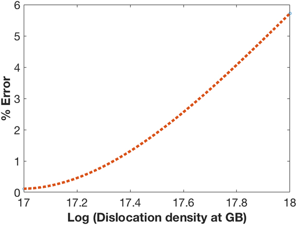
Note that the integration of ΔSSD(x) is required to be null, as this is the deviation about the average SSD dislocation density. This completes the analysis demonstrating under what conditions the Taylor hardening law is consistent with the linear SGP flow rule when the spatial variation of the dislocation density in general is less than or equal to the average indentation dislocation density. Connecting this analysis with Eqs. (2)–(4) is of considerable interest as well. Using the sequential Taylor series again for Eq. (4a) gives
 $${H_0}\sqrt {1 + {{{h^*} + h_{{\rm{gb}}}^{\rm{*}}} \over {{f^3}h}}} \cong {H_0}\left( {1 + {{{h^*}} \over {2{f^3}h}} + {{h_{{\rm{gb}}}^*} \over {2{f^3}h}}} \right)\quad .$$
For intrinsic ISE, comparison of Eqs. (A.9) and (A.7) confirms the Evans et al. analysis [Reference Evans and Hutchinson59] that  $l \propto {1 \!\left/{\vphantom{1 {\sqrt {\overline {{\rho _{{\rm{SSD}}}}} } }}}\right.{\sqrt {\overline {{\rho _{{\rm{SSD}}}}} } }}$ and that
 ${h^*} \propto {1 / {\left( {b\overline {{\rho _{{\rm{SSD}}}}} } \right)}}$ and that the two length scales are not equivalent.
Appendix B. Consideration of the limiting case for the Schmid factor term, Δm.
The Schmid factor term,  $\Delta m = {{{m_1} - {m_2}} \over {{m_1}{m_2}}}$, defined in Eq. (13) is difficult to analytically determine for Berkovich nanoindentation as the resulting stress tensor is multidimensional and, in particular, non-uniform. However, it is possible to consider a limiting case for an effective Δm. There are statistically significant hardness differences between the grain surfaces (Table B1), and we take the softest of the observed grain to have an effective Schmid factor of 0.5. The hardness difference between the softest grain and the other grains is then attributed to a difference in the Berkovich effective Schmid factor through the relations Eqs. (B.1) and (B.2). The analysis can be taken a step further by noting that there is a correlation between the adjacent grain hardness difference in Fig. B1 and the increase in grain boundary hardness relative to the average of the adjacent grain hardness or relative to the hardness of the hardest grain. Not only does this limiting case analysis provide a range of Δm values for examination of curve fitting results but also provides an additional qualitative test for the proposed concept that the hardening due to local indentation of the grain boundary is related to the Ashby plastic incompatibility argument. The results of these measurements are shown in Table B1. The limiting case values for Δm that result from the differences in grain hardness [from Eq. (B.2)] are shown in Fig. B2(a). In Fig. B2(b), the trend of an increase in grain boundary hardness with increasing Δm is demonstrated (relative to the average grain hardness).
Limiting case analysis for the effective Schmid factor.
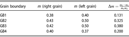
 $$H \propto \sigma \propto {1 \over m}\quad ,$$
 $${m_{{\rm{grain}}\left( {\rm{i}} \right)}} = {m_{{\rm{softest}}\;{\rm{grain}}}} \times {{{H_{{\rm{softest}}\;{\rm{grain}}}}} \over {{H_{{\rm{grain}}\left( {\rm{i}} \right)}}}}\quad .$$
Representative Nix–Gao plots for comparing grain boundary chopping indentation (green) with adjacent grain interiors (black and orange) for (a) GB1, (b) GB22, (c) GB3, and (d) GB4.
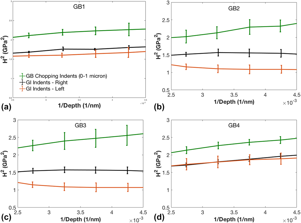
(a) Correlating difference in hardness of adjacent grains (delta H) with the limiting case for (Δm) Eq. (B.2). (b) Correlating difference in hardness between grain boundary and harder adjacent grain interior (delta GH) with estimated (Δm).
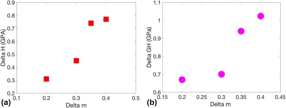
Figure B2 offers some support for the idea that plastic incompatibility at the grain boundary, as described by Ashby [Reference Ashby3], is the root cause of the experimental observations in Fig. 7. According to the Ashby theory, the GND dislocation density and plastic strain should increase as Δm increases, and this is indeed the trend of increasing hardness with increasing Δm observed in Fig. B2(b).
This range in Δm considered in Fig. B2 does allow for the further interpretation of Eq. (8) and subsequently Eq. (5) using the Ashby boundary condition, Eq. (10), γ = γ1 − γ2 = εp × Δm such that
 $$\eqalign{{\gamma / {bf}}\left( {{{\left( {1 - {{\rm{e}}^{ - n}}} \right)} \over n}} \right) = {{{\varepsilon _{\rm{p}}}\Delta m} / {bf}}\left( {{{\left( {1 - {{\rm{e}}^{ - n}}} \right)} \over n}} \right) \cr= 4.5 \times {10^8}\;{{\rm{m}}^{ - 1}}\quad .$$
Taking the usual characteristic strain for Berkovich indentation as εp ∼ 0.1, Δm ∼ 0.3 from Fig. B2, and f ∼ 2.0 to 3.2 from the Eq. (5) Hall–Petch coefficient gives from Eq. (B.3) that n ∼ 0.2 to 0.45. The relatively small value of n and f found here would suggest that the plastic zone due to the grain boundary deformation is localized at the grain boundary but relatively uniform, consistent with the measurements of Vachhani [Reference Vachhani, Doherty and Kalidindi20] and the analysis of Evers et al. [Reference Evers, Parks, Brekelmans and Geers48]. It is also noted that this value of f suggesting grain boundary plastic zone localization [f ∼ 1/tan(θ)] would be specific to the Ashby mechanism caused by the local grain boundary indentation geometry described in this paper, as opposed to the value of f from considerations of remote indentation extrinsic ISE [Reference Xiao, Terentyev, Chen, Yua, Chen, Bakaev and Duan22] or considerations of the intrinsic ISE [Reference Feng and Nix61] as these other ISE are attributed to different deformation processes.
Appendix C. Continuum SGP Approximation.
The purpose of this appendix is to examine the sources of error associated with substitution of a proposed plastic strain field into an SGP flow rule to estimate the resulting equivalent stress. Certainly, the simple substitution approach has been done previously by other investigators, specifically Wei et al. [Reference Wei, Konstantinidis, Qi and Aifantis58] and Stoelken et al. [Reference Stoelken and Evans65]. It should also be noted even the more involved plastic potential minimization approach has been utilized by presupposing the general form of the displacement field, where the coefficients are then determined to satisfy the boundary conditions and to minimize the potential [Reference Niordson and Hutchinson66].
The formulation of the SGP continuum analysis adapted to the linear analysis pursued here was recently described by Wei et al. [Reference Wei, Konstantinidis, Qi and Aifantis58], who defined a general form for the continuum SGP equivalent stress as
 $${\sigma _{\rm{e}}} = \beta \left( {\overline {{\varepsilon _{\rm{p}}}} + {l_1}{{\left[ {\vec{\nabla }\overline {{\varepsilon _{\rm{p}}}} \Delta \vec{\nabla }\overline {{\varepsilon _{\rm{p}}}} } \right]}^{\rm{q}}} + {l_2}{\nabla ^2}\overline {{\varepsilon _{\rm{p}}}} } \right)\quad ,$$
where we take the characteristic length l 2 = 0 and the exponent q = 1/2, as represented by Eqs. (A.1) and (A.3). The equivalent stress and plastic strain measures are defined as 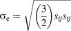 ${\sigma _{\rm{e}}} = \sqrt {\left( {{3 \over 2}} \right){s_{ij}}{s_{ij}}}$ and
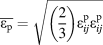 $\overline {{\varepsilon _{\rm{p}}}} = \sqrt {\left( {{2 \over 3}} \right)\varepsilon _{ij}^{\rm{p}}\varepsilon _{ij}^{\rm{p}}}$, where s ij is the deviatoric stress component and
 $\varepsilon _{ij}^{\rm{p}}$ is a component of the plastic stress tensor. The equivalent stress, σe, is then a function and the magnitude of the gradient squared
 $\left( {\vec{\nabla }\overline {{\varepsilon _{\rm{p}}}} \cdot \vec{\nabla }\overline {{\varepsilon _{\rm{p}}}} } \right)$ as utilized in Eq. (C.1). Here, we will consider a two-dimensional, plastic strain field based on a displacement potential satisfying the biharmonic partial differential equation, so that
 ${\left( {\vec{\nabla }\overline {{\varepsilon _{\rm{p}}}} \cdot \vec{\nabla }\overline {{\varepsilon _{\rm{p}}}} } \right)^{{1 / 2}}} = \left( {{1 / 2}} \right)\left( {\left| {{\nabla _x}\overline {{\varepsilon _{\rm{p}}}} } \right| + \left| {{\nabla _y}\overline {{\varepsilon _{\rm{p}}}} } \right|} \right)$. Thus, Eq. (C.1a) can be rewritten as follows:
 $${\sigma _{\rm{e}}} = \beta \left( {\overline {{\varepsilon _{\rm{p}}}} + {{{l_1}} \over 2}\left( {\left| {{\nabla _x}\overline {{\varepsilon _{\rm{p}}}} } \right| + \left| {{\nabla _y}\overline {{\varepsilon _{\rm{p}}}} } \right|} \right)} \right)\quad .$$
The simplest approach [Reference Wei, Konstantinidis, Qi and Aifantis58, Reference Stoelken and Evans65], but not the most accurate, would be to substitute a plastic strain field that satisfied all boundary, compatibility, and equilibrium conditions directly into Eq. (C.1b) to determine the equivalent stress. The error in the simple approach arises from a neglect of the elastic strains, essentially assuming that all strains are plastic. The error here can be estimated by following [Reference Engelen67], taking the general expression for an elastic–plastic solid in the plastic zone (small strain) as
 $${\varepsilon _{ij}} = {3 \over {2E}}{\dot{s}_{ij}} + {3 \over 2}{\dot{\varepsilon }_{\rm{p}}}{{{s_{ij}}} \over {{\sigma _{\rm{e}}}}}\quad ,$$
with εij as the total strain tensor. The boundary conditions of the displacements and strains due to the indentation of the grain boundary will be prescribed, from which the total strain tensor can be determined using the Marguerre displacement function with ν = 1/2 for plastic deformation. In this manner, the compatibility conditions relating displacement and strain will be satisfied, along with the conditions for stress component equilibrium. A compressive plastic displacement of magnitude h will be applied to the surface parallel the x axis, with the surface height at/(2ω), to cause plastic displacements at the grain boundary lying on the xz plane at y = 0 in accordance with the Ashby model [Eq. (15)] [Reference Ashby3]. The simplest, relevant displacement potential that will satisfy the boundary, compatibility, and equilibrium conditions is then proposed as:
 $$\Psi = A{x^2}y + B{{\rm{e}}^{ - \omega y}}\sin \left( {\omega x} \right)\quad ,$$
where A and B are integration constants and ω is a spatial frequency, all to be determined by boundary conditions. The coefficient, A, in Eq. (C.3a) can be considered to represent the intrinsic aspect of the indentation, while the coefficient, B, represents the extrinsic effect of the grain boundary. Equation (C.3a) may be used to obtain an approximate value for the total strain tensor components, εij, as
 $${\varepsilon _{{\rm{xx}}}} = {4 \over 3}\left( { - {\nabla _{xxy}}\Psi + {1 \over 2}{\nabla _{yyy}}\Psi } \right)\quad ,$$
 $${\varepsilon _{yy}} = {4 \over 3}\left( {{5 \over 2}{\nabla _{xxy}}\Psi + {\nabla _{yyy}}\Psi } \right)\quad ,$$
 $${\varepsilon _{xy}} = {4 \over 3}\left( {{\nabla _{xxx}}\Psi + {1 \over 2}{\nabla _{xyy}}\Psi } \right)\quad .$$
To zero order in Bω3, the approximate relation −2.5s xx ∼ s yy will hold if the elastic (and plastic) strains are proportional to the total strains, giving σe ∼ 3.3 |s xx|. This relation allows for the substitution of σe for s xx in Eq. (C.2), which then gives the x total strain tensor component as
 $$- {\varepsilon _{xx}}\sim - {1 \over 2}\left( {{{{\sigma _{\rm{e}}}} \over E} + {\varepsilon _{\rm{p}}}} \right)\quad .$$
Further substitution of Eq. (C.1b) for σe and Eq. (C.3b) for εxx in Eq. (C.4) gives a linear, first-order partial differential equation similar to that presented in the appendices of Evans et al. [Reference Evans and Hutchinson59] for lower order theory. The linear, first-order partial differential equation obtained from Eq. (C.4) has a solution to zero order in  $\left( {{\beta \over E}} \right)$ as
 $$\overline {{\varepsilon _{\rm{p}}}} = 2\left| {{\varepsilon _{xx}}} \right| + {C_1}f\left( {x,y} \right)\quad ,$$
where C 1 is an integration constant and the function f(x,y) exponentially decays in the x direction with length scale, l. This integration constant, C 1, could be used to “correct” any nonphysical boundary condition resulting for the higher order (gradient induced) stress, such as setting free surface tractions resulting from gradient terms to null value. However, the proposed model has no free surfaces; therefore, C 1 is taken to be zero. We also note the full solution to Eq. (C.1) is of particular interest, because it introduces a mathematically rich environment for physical analyses, but the full solution not considered further in this paper. Simply put, the Eq. (C.1) solution with relative error 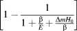 $\left[ {1 - {1 \over {1 + {\beta \over E} + {{\Delta m{H_0}} \over \beta }}}} \right]$ gives the plastic strain measure as proportional to the x-component of the imposed total strain tensor components. As such,
 $$\overline {{\varepsilon _{\rm{p}}}} = 4A + 3B{\omega ^3}\sin \left( {\omega x} \right)\exp \left( { - \omega y} \right)\quad .$$
This is essentially the same simplified approach utilized by Stoelken et al. [Reference Stoelken and Evans65] and Engelen [Reference Engelen67], where the plastic strain measure is proportional to a component of the total strain tensor. The solution for the individual strain tensor components is considered for y > 0. The solution for y < 0 could also be written in the form of Eq. (C.2) and, thus, mirror the y > 0 solution with a change in sign of the exponential argument. This interpretation of the solution could allow the normal components of plastic strain to be continuous, but not differentiable, across the grain boundary.
The variables A, B, and ω can be determined from the boundary conditions expressed by Eqs. (C.7a)–(C.7c). Equation (C.7a) is the rendition of Eq. (15) for the two-dimensional plastic strain measure, where the subscript B = 0 on the lhs refers to the plastic strain measure that would occur without the grain boundary present:
 $$\overline {{\varepsilon _{{\rm{p,B = 0}}{\rm{.}}}}} {{\Delta m} \over L} = {\left. {\nabla \overline {{\varepsilon _{\rm{p}}}} } \right|_{y = 0}}\quad ,$$
and the trigonometric terms in Eq. (C.7a) are averaged over the length π/(2ω). Equation (C.7b) specifies that the plastic displacement at the surface is controlled by the geometry of the indenter, which is uniform in this simple model. Although simplistic in presentation, this boundary condition results in the sine function dependence for Ψ in Eq. (C.3a); thus, there is no y dependence on the plastic displacement along the surface (x = π/(2ω)) due to the grain boundary:
 $${\left. {{u_x}} \right|_{x = {\pi / {\left( {2\omega } \right)}}}} = - h\quad .$$
The boundary condition in Eq. (C.7c) guarantees that H will not show a grain boundary or a size effect when the grain boundary is not present (Δm = 0) and/or h becomes very large:
 $${\left. {\beta \overline {{\varepsilon _{\rm{p}}}} } \right|_{x = {\pi \!\left/{\vphantom{\pi {(2\omega )}}}\right.{(2\omega )}},\Delta m = 0}} = {H_0}\quad ,$$
where the exponential terms in Eq. (C.7c) are averaged over the length π/(2ω).
The stress contribution from the grain boundary due to the averaged equivalent stress at the surface is then obtained from Eqs. (C.1)–(C.7) by averaging the exponential y dependent term over the length π/(2ω) to give the stress contribution due to the coefficient B and the extrinsic ISE as
 $${\left[ {{{\left. {\overline {{\sigma _{\left( {{\rm{gb}}} \right)}}} } \right|}_{x = {\pi \!\left/{\vphantom{\pi {(2\omega )}}}\right.{(2\omega )}}}}} \right]_{{\rm{extrinsic}}}} = \left( {{{0.12n{H_0}{l_1}\Delta m} \over h}} \right) + 0.02n\beta \Delta m\quad ,$$
where L = h/n. Equation (C.8) has an inverse h dependence and, thus, describes the extrinsic ISE. Drawing from the concepts leading to Eq. (A.8), the total stress from the addition of the intrinsic and extrinsic components of the deformation is then used to estimate H:
 $$H = {\left[ {{H_0}\left( {1 + {{{h^*}} \over {2{f^3}h}}} \right)} \right]_{{\rm{intrinsic}}}} + {\left[ {{{\left. {\overline {{\sigma _{\left( {{\rm{gb}}} \right)}}} } \right|}_{x = {\pi \!\left/{\vphantom{\pi {(2\omega )}}}\right.{(2\omega )}}}}} \right]_{{\rm{extrinsic}}}}\quad .$$
As a final examination of physical validity, we follow the transparent (but highly approximate) demonstration of strain gradient effects in Ref. [Reference Evans and Hutchinson59]. To develop this physical picture of the Ashby mechanism within the context of SGP, Eqs. (12)–(15) are examined in terms the plastic strain and plastic strain gradient, which develops on the grain boundary due to the indentation process. From Eq. (12),
 $${\varepsilon _{{\rm{p}}\left( {{\rm{gb}}} \right)}} = {{{u_{{\rm{gb}}}}} \over h} = \left( {{{{H_0}} \over \beta }} \right)\Delta m\quad .$$
And Eq. (12) with Eq. (15) is rewritten as follows:
 $${{{\rm{d}}{\varepsilon _{{\rm{p}}\left( {{\rm{gb}}} \right)}}} \over {{\rm{d}}y}} = {{{u_{{\rm{gb}}}}} \over {{h^2}}} = \left( {{{{H_0}} \over {\beta h}}} \right)\Delta m\quad .$$
For a one-dimensional gradient plasticity, linear flow rule, Eq. (A.1), Eqs. (C.10), and (C.11) may be rewritten as an estimate of the contribution of the grain boundary to the equivalent stress
 $${\sigma _{{\rm{e}}\left( {{\rm{gb}}} \right)}} = \beta \Delta m\left( {{{{H_0}} \over \beta } + l{{{H_0}} \over {\beta h}}} \right)\quad ,$$
which has the same general form as Eq. (C.8). Finally, writing Eq. (C.12) in the form of Eqs. (A.1)–(A.7) for the Taylor flow stress relates the mechanical behavior to the dislocation density.
 $$\eqalign{{\sigma _{{\rm{e}}\left( {{\rm{gb}}} \right)}} = \beta b\Delta m\left( {{{{H_0}} \over {\beta b}} + {{\beta b} \over {2{H_0}}}{{{H_0}} \over {\beta {b^2}h}}} \right) \cr= \beta b\left( {\sqrt {\overline {{\rho _{\left( {{\rm{gb}}} \right)}}} } + {{\overline {{\rho _{{\rm{GND}}\left( {{\rm{gb}}} \right)}}} } \over {2\sqrt {\overline {{\rho _{{\rm{SSD}}}}} } }}} \right)\quad .$$