


1 Introduction
Observations made in the space environment consistently show plasma particles with velocity distributions that have non-thermal tails, and frequently with anisotropies which are not well described by Maxwellian distributions or bi-Maxwellian distributions. These observed non-thermal features are usually described by distributions featuring power-law tails, which are generically known as Kappa distributions (Olbert Reference Olbert, Carovillano, McClay and Radoski1968; Vasyliunas Reference Vasyliunas1968; Summers & Thorne Reference Summers and Thorne1991; Mace & Hellberg Reference Mace and Hellberg1995; Leubner & Schupfer Reference Leubner and Schupfer2000, Reference Leubner and Schupfer2001; Leubner Reference Leubner2002, Reference Leubner2004).
It is common knowledge that Kappa distributions have been introduced to describe non-thermal features of velocity distributions in the pioneering works by Olbert (Reference Olbert, Carovillano, McClay and Radoski1968) and Vasyliunas (Reference Vasyliunas1968), but are nowadays written in terms of different mathematical distributions. Isotropic Kappa distributions are usually written in terms of two different forms, one which can be found in Summers & Thorne (Reference Summers and Thorne1991), Mace & Hellberg (Reference Mace and Hellberg1995), and the other which can be found in Leubner (Reference Leubner2002, Reference Leubner2004). These two different forms of Kappa distributions have been used by the plasma physics community, and have been the subject of a number of theoretical discussion in recent years (Hellberg et al. Reference Hellberg, Mace, Baluku, Kourakis and Saini2009; Hapgood et al. Reference Hapgood, Perry, Davies and Denton2011; Livadiotis & McComas Reference Livadiotis and McComas2013; Livadiotis Reference Livadiotis2015). Anisotropic particle distributions can also have extended non-thermal features, which are also usually described in terms of two different forms. In one of these forms, which is known as a bi-Kappa distribution (BK), the anisotropy is associated with parameters related to the temperature, with a single kappa index (Leubner & Schupfer Reference Leubner and Schupfer2000, Reference Leubner and Schupfer2001; Lazar & Poedts Reference Lazar and Poedts2009a ,Reference Lazar and Poedts b ; Lazar, Poedts & Schlickeiser Reference Lazar, Poedts and Schlickeiser2011; Lazar Reference Lazar2012; Lazar & Poedts Reference Lazar and Poedts2014). In the second form, which is known as product-bi-Kappa distribution (PBK), anisotropic kappa indexes are introduced, in addition to anisotropic temperature parameters (Lazar et al. Reference Lazar, Pierrard, Poedts and Schlickeiser2012; Lazar & Poedts Reference Lazar and Poedts2014; dos Santos, Ziebell & Gaelzer Reference dos Santos, Ziebell and Gaelzer2014, Reference dos Santos, Ziebell and Gaelzer2015, Reference dos Santos, Ziebell and Gaelzer2016).
In any of the mentioned forms, Kappa distributions are frequently employed in an empirical way, fitting observed distributions, as in Maksimovic, Pierrard & Riley (Reference Maksimovic, Pierrard and Riley1997). It is also possible to find theoretical studies dedicated to basic fundamental properties of Kappa distributions (Hellberg & Mace Reference Hellberg and Mace2002; Mace & Hellberg Reference Mace and Hellberg2003; Hau & Fu Reference Hau and Fu2007; Hau, Fu & Chuang Reference Hau, Fu and Chuang2009; Hellberg et al. Reference Hellberg, Mace, Baluku, Kourakis and Saini2009; Mace & Hellberg Reference Mace and Hellberg2009), or to the relationship between Kappa distributions and wave phenomena in plasmas. Among studies with the latter characteristics, mention can be made of studies on low-frequency electromagnetic instabilities, dealing with the ion-cyclotron instability, as in Lazar (Reference Lazar2012), Lazar & Poedts (Reference Lazar and Poedts2014), or with the ion firehose instability, as in Lazar & Poedts (Reference Lazar and Poedts2009a ,Reference Lazar and Poedts b ), Lazar et al. (Reference Lazar, Poedts and Schlickeiser2011), or with Langmuir waves, as in Thorne & Summers (Reference Thorne and Summers1991), or obliquely propagating generalized Langmuir waves, as in Mace & Hellberg (Reference Mace and Hellberg2003), or studies based on a quasi-linear formulation aiming to investigate bursty solar wave emission phenomena, as in Li & Cairns (Reference Li and Cairns2014), or analyses on the effects of superthermal particles on waves in magnetized plasmas, in space environment (Hellberg, Mace & Cattaert Reference Hellberg, Mace and Cattaert2006).
As mentioned, the Kappa distributions used in the literature are frequently represented in different forms, which have in common the power-law dependence for high values of velocity. In the present paper, we use a generic form of Kappa distribution, which in particular cases can reproduce the two widely used forms already mentioned, and consider the isotropic and the anisotropic cases, discussing in each case the dispersion relations for Langmuir (L) and ion-sound (S) waves in a systematic way. The description of these waves is obtained from the dispersion relation for electrostatic (ES) waves, given by
 $\unicode[STIX]{x1D700}_{zz}=0$
, where
 $$\begin{eqnarray}\unicode[STIX]{x1D700}_{zz}=1-\frac{1}{z^{2}}\mathop{\sum }_{\unicode[STIX]{x1D6FD}}\frac{\unicode[STIX]{x1D714}_{p\unicode[STIX]{x1D6FD}}^{2}}{\unicode[STIX]{x1D6FA}_{\ast }^{2}}\frac{1}{n_{\unicode[STIX]{x1D6FD}0}}\left(I-J(0,0,2;f_{\unicode[STIX]{x1D6FD}})\right).\end{eqnarray}$$
The
 $J(0,0,2;f_{\unicode[STIX]{x1D6FD}})$
in (1.1) is a particular case of a generic integral form, which is valid both for magnetized and unmagnetized environments,
 $$\begin{eqnarray}J(n,m,h;f_{\unicode[STIX]{x1D6FD}})\equiv z\int \,\text{d}^{3}u\,\frac{u_{\Vert }^{h}u_{\bot }^{2(m-1)}u_{\bot }L(f_{\unicode[STIX]{x1D6FD}})}{z-nr_{\unicode[STIX]{x1D6FD}}-q_{\Vert }u_{\Vert }},\end{eqnarray}$$
and
 $I$
is defined as follows
 $$\begin{eqnarray}I=\int \,\text{d}^{3}u\,\frac{u_{\Vert }}{u_{\bot }}{\mathcal{L}}(f_{\unicode[STIX]{x1D6FD}}).\end{eqnarray}$$
In these expressions,
 ${\mathcal{L}}$
and
 $L$
are differential operators,
 $$\begin{eqnarray}\displaystyle & \displaystyle {\mathcal{L}}=\left(u_{\Vert }\frac{\unicode[STIX]{x2202}}{\unicode[STIX]{x2202}u_{\bot }}-u_{\bot }\frac{\unicode[STIX]{x2202}}{\unicode[STIX]{x2202}u_{\Vert }}\right) & \displaystyle\end{eqnarray}$$
 $$\begin{eqnarray}\displaystyle & \displaystyle L=\left[\left(1-\frac{q_{\Vert }}{z}u_{\Vert }\right)\frac{\unicode[STIX]{x2202}}{\unicode[STIX]{x2202}u_{\bot }}+\frac{q_{\Vert }}{z}u_{\bot }\frac{\unicode[STIX]{x2202}}{\unicode[STIX]{x2202}u_{\Vert }}\right] & \displaystyle\end{eqnarray}$$
and the following dimensionless variables have been introduced
 $$\begin{eqnarray}\displaystyle z=\frac{\unicode[STIX]{x1D714}}{\unicode[STIX]{x1D6FA}_{\ast }},\quad u_{\Vert ,\bot }=\frac{v_{\Vert ,\bot }}{v_{\ast }},\quad q_{\Vert }=\frac{k_{\Vert }v_{\ast }}{\unicode[STIX]{x1D6FA}_{\ast }},\quad r_{\unicode[STIX]{x1D6FD}}=\frac{\unicode[STIX]{x1D6FA}_{\unicode[STIX]{x1D6FD}}}{\unicode[STIX]{x1D6FA}_{\ast }}, & & \displaystyle\end{eqnarray}$$
where
 $\unicode[STIX]{x1D714}$
and
 $k$
are the wave angular frequency and wavenumber, respectively,
 $\unicode[STIX]{x1D6FA}_{\unicode[STIX]{x1D6FD}}$
is the angular cyclotron frequency for particles of species
 $\unicode[STIX]{x1D6FD}$
, and
 $\unicode[STIX]{x1D6FA}_{\ast }$
and
 $v_{\ast }$
are some characteristic angular frequency and velocity, respectively. Moreover,
 $\unicode[STIX]{x1D714}_{p\unicode[STIX]{x1D6FD}}$
is the angular plasma frequency and
 $f_{\unicode[STIX]{x1D6FD}}$
the velocity distribution function, for particles of species
 $\unicode[STIX]{x1D6FD}$
. In the present case, for the study of ES waves, it is convenient to assume
 $\unicode[STIX]{x1D6FA}_{\ast }=\unicode[STIX]{x1D714}_{pe}$
and
 $v_{\ast }=v_{e}$
, the angular electron plasma frequency and the electrons thermal velocity, respectively. As usual, the thermal velocities for particles of species
 $\unicode[STIX]{x1D6FD}$
are defined as
 $v_{\unicode[STIX]{x1D6FD}}^{2}=2T_{\unicode[STIX]{x1D6FD}}/m_{\unicode[STIX]{x1D6FD}}$
, where
 $T_{\unicode[STIX]{x1D6FD}}$
is a parameter which characterizes the temperature. Notice that in the present notation the dependence of the velocity distribution functions appear in the dispersion relation through the integral quantities (1.2) and (1.3).
The paper is organized as follows. In § 2 we introduce a generic form of Kappa distribution, considering the isotropic case and also the anisotropic BK and PBK cases of this generic distribution. Section 2 also presents analytical results for the dispersion relation of L and S waves, both exact and approximated, obtained with the use of these generic distributions. In § 3 we consider two particular isotropic cases of the generic distribution introduced in § 2, and present the corresponding analytical expressions for the dispersion relation of L and S waves, both exact and approximated. In § 4 we introduce and discuss anisotropic forms of Kappa distribution which are particular cases of the generic distribution presented in § 2, and also present the corresponding exact and approximated forms of the dispersion relations for L and S waves. In § 5 we present some results obtained from numerical solution of the dispersion relation obtained for different forms of the velocity distribution, and also present some results obtained from particle-in-cell (PIC) simulations, regarding electrostatic fluctuations. Section 6 summarizes the results obtained.
2 Generic forms of isotropic and anisotropic Kappa distributions and the corresponding dispersion relations for Langmuir and ion-sound waves
Let us assume the following form of isotropic Kappa distribution for ions and electrons (Gaelzer & Ziebell Reference Gaelzer and Ziebell2014, Reference Gaelzer and Ziebell2016),
 $$\begin{eqnarray}\displaystyle f_{\unicode[STIX]{x1D6FD}}(\boldsymbol{v})=\frac{n_{\unicode[STIX]{x1D6FD}0}}{\unicode[STIX]{x03C0}^{3/2}\unicode[STIX]{x1D705}_{\unicode[STIX]{x1D6FD}}^{3/2}w_{\unicode[STIX]{x1D6FD},\unicode[STIX]{x1D705}}^{3}}\frac{\unicode[STIX]{x1D6E4}(\unicode[STIX]{x1D705}_{\unicode[STIX]{x1D6FD}}+\unicode[STIX]{x1D6FC}_{\unicode[STIX]{x1D6FD}})}{\unicode[STIX]{x1D6E4}(\unicode[STIX]{x1D705}_{\unicode[STIX]{x1D6FD}}+\unicode[STIX]{x1D6FC}_{\unicode[STIX]{x1D6FD}}-3/2)}\left(1+\frac{v^{2}}{\unicode[STIX]{x1D705}_{\unicode[STIX]{x1D6FD}}w_{\unicode[STIX]{x1D6FD},\unicode[STIX]{x1D705}}^{2}}\right)^{-(\unicode[STIX]{x1D705}_{\unicode[STIX]{x1D6FD}}+\unicode[STIX]{x1D6FC}_{\unicode[STIX]{x1D6FD}})}, & & \displaystyle\end{eqnarray}$$
where
 $\unicode[STIX]{x1D6FC}_{\unicode[STIX]{x1D6FD}}$
is a constant and
 $w_{\unicode[STIX]{x1D6FD},\unicode[STIX]{x1D705}}$
is a parameter with the same physical dimension as the particle thermal velocity, and which reduces to the Maxwellian thermal velocity in the limit
 $\unicode[STIX]{x1D705}_{\unicode[STIX]{x1D6FD}}\rightarrow \infty$
. The distribution function given by (2.1) is normalized such that
 $\int \,\text{d}^{3}v\,f_{\unicode[STIX]{x1D6FD}}=n_{\unicode[STIX]{x1D6FD}0}$
.
The quantity
 $I$
in (1.1) vanishes in the case of an isotropic distribution, as is the case of (2.1). After evaluation of the
 $J(0,0,2;f_{\unicode[STIX]{x1D6FD}})$
integral for this distribution function (details can be seen in appendix A), the dispersion relation for ES waves propagating along a given direction denominated as
 $z$
axis, with wavenumber
 $\boldsymbol{k}=k_{\Vert }\,\boldsymbol{e}_{\boldsymbol{z}}$
, can be written as follows,
 $$\begin{eqnarray}\displaystyle & & \displaystyle \displaystyle 1+2\mathop{\sum }_{\unicode[STIX]{x1D6FD}}\frac{\unicode[STIX]{x1D714}_{p\unicode[STIX]{x1D6FD}}^{2}}{\unicode[STIX]{x1D714}^{2}}(\unicode[STIX]{x1D701}_{\unicode[STIX]{x1D6FD}}^{0})^{2}\left(\frac{\unicode[STIX]{x1D705}_{\unicode[STIX]{x1D6FD}}+\unicode[STIX]{x1D6FC}_{\unicode[STIX]{x1D6FD}}-3/2}{\unicode[STIX]{x1D705}_{\unicode[STIX]{x1D6FD}}}+\frac{\unicode[STIX]{x1D6E4}(\unicode[STIX]{x1D705}_{\unicode[STIX]{x1D6FD}}+\unicode[STIX]{x1D6FC}_{\unicode[STIX]{x1D6FD}})}{\unicode[STIX]{x1D705}_{\unicode[STIX]{x1D6FD}}\unicode[STIX]{x1D6E4}(\unicode[STIX]{x1D705}_{\unicode[STIX]{x1D6FD}})}\right.\nonumber\\ \displaystyle & & \displaystyle \displaystyle \quad \times \,\left.\frac{\unicode[STIX]{x1D6E4}(\unicode[STIX]{x1D705}_{\unicode[STIX]{x1D6FD}}-1/2)}{\unicode[STIX]{x1D6E4}(\unicode[STIX]{x1D705}_{\unicode[STIX]{x1D6FD}}+\unicode[STIX]{x1D6FC}_{\unicode[STIX]{x1D6FD}}-3/2)}\unicode[STIX]{x1D701}_{\unicode[STIX]{x1D6FD}}^{0}Z_{\unicode[STIX]{x1D705}_{\unicode[STIX]{x1D6FD}}}^{(\unicode[STIX]{x1D6FC}_{\unicode[STIX]{x1D6FD}})}(\unicode[STIX]{x1D701}_{\unicode[STIX]{x1D6FD}}^{0})\right)=0,\end{eqnarray}$$
where
 $\unicode[STIX]{x1D701}_{\unicode[STIX]{x1D6FD}}^{0}=\unicode[STIX]{x1D714}/(k_{\Vert }w_{\unicode[STIX]{x1D6FD},\unicode[STIX]{x1D705}})$
, and where
 $Z_{\unicode[STIX]{x1D705}_{\unicode[STIX]{x1D6FD}}}^{(\unicode[STIX]{x1D6FC}_{\unicode[STIX]{x1D6FD}})}$
is obtained from the general definition
 $$\begin{eqnarray}\displaystyle Z_{\unicode[STIX]{x1D705}}^{(m)}(\unicode[STIX]{x1D709}) & = & \displaystyle \frac{\text{i}\unicode[STIX]{x1D6E4}(\unicode[STIX]{x1D705})\unicode[STIX]{x1D6E4}(\unicode[STIX]{x1D705}+m+1/2)}{\unicode[STIX]{x1D705}^{1/2}\unicode[STIX]{x1D6E4}(\unicode[STIX]{x1D705}-1/2)\unicode[STIX]{x1D6E4}(\unicode[STIX]{x1D705}+m+1)}\nonumber\\ \displaystyle & & \displaystyle \times \,_{2}F_{1}\left[1,2\unicode[STIX]{x1D705}+2m;\unicode[STIX]{x1D705}+m+1;\frac{1}{2}\left(1+\frac{\text{i}\unicode[STIX]{x1D709}}{\unicode[STIX]{x1D705}^{1/2}}\right)\right],\end{eqnarray}$$
valid for
 $\unicode[STIX]{x1D705}>-m-1/2$
, for
 $m=\unicode[STIX]{x1D6FC}$
.
An approximated form of the dispersion relation of L waves can be obtained if we take into account that the L waves are waves with large phase velocity,
 $|\unicode[STIX]{x1D701}_{\unicode[STIX]{x1D6FD}}^{0}|\gg 1$
. Expanding the integrand of the
 $J(0,0,2;f_{\unicode[STIX]{x1D6FD}})$
integral (details can be seen in appendix A), the dispersion relation for L waves turns out to be given as follows, in terms of dimensional quantities,
 $$\begin{eqnarray}1-\mathop{\sum }_{\unicode[STIX]{x1D6FD}}\frac{\unicode[STIX]{x1D714}_{p\unicode[STIX]{x1D6FD}}^{2}}{\unicode[STIX]{x1D714}^{2}}\left(1+\frac{3}{2}\frac{\unicode[STIX]{x1D705}_{\unicode[STIX]{x1D6FD}}}{\unicode[STIX]{x1D705}_{\unicode[STIX]{x1D6FD}}+\unicode[STIX]{x1D6FC}_{\unicode[STIX]{x1D6FD}}-5/2}\frac{1}{(\unicode[STIX]{x1D701}_{\unicode[STIX]{x1D6FD}}^{0})^{2}}\right)=0.\end{eqnarray}$$
In order to obtain an approximated expression to be used for S waves, we consider the distribution function given by (2.2) and waves satisfying the conditions
 $|\unicode[STIX]{x1D701}_{e}^{0}|\ll 1$
and
 $|\unicode[STIX]{x1D701}_{i}^{0}|\gg 1$
. By expansion of the integrand of the
 $J(n,m,h,f_{\unicode[STIX]{x1D6FD}})$
integrals considering the appropriate limits (details can be seen in appendix A), the dispersion relation for S waves can be given as follows
 $$\begin{eqnarray}\displaystyle 1-\frac{\unicode[STIX]{x1D714}_{pi}^{2}}{\unicode[STIX]{x1D714}^{2}}\left(1+\frac{3}{2}\frac{\unicode[STIX]{x1D705}_{i}}{\unicode[STIX]{x1D705}_{i}+\unicode[STIX]{x1D6FC}_{i}-5/2}\frac{1}{(\unicode[STIX]{x1D701}_{i}^{0})^{2}}\right)+2\frac{\unicode[STIX]{x1D714}_{pe}^{2}}{\unicode[STIX]{x1D714}^{2}}\frac{\unicode[STIX]{x1D705}_{e}+\unicode[STIX]{x1D6FC}_{e}-3/2}{\unicode[STIX]{x1D705}_{e}}(\unicode[STIX]{x1D701}_{e}^{0})^{2}=0. & & \displaystyle\end{eqnarray}$$
Particular cases of the distribution (2.1), which correspond to forms of Kappa distributions which are widely used in plasma physics investigations, can be obtained by suitable choice of the parameters
 $\unicode[STIX]{x1D6FC}_{\unicode[STIX]{x1D6FD}}$
and
 $w_{\unicode[STIX]{x1D6FD},\unicode[STIX]{x1D705}}$
. These particular cases will be considered in the sections which follow.
A generic form of BK distribution can also be defined, similar to the distribution given by (2.1) (Gaelzer, Ziebell & Meneses Reference Gaelzer, Ziebell and Meneses2016),
 $$\begin{eqnarray}\displaystyle f_{\unicode[STIX]{x1D6FD}}(\boldsymbol{v})=\frac{n_{\unicode[STIX]{x1D6FD}0}}{\unicode[STIX]{x03C0}^{3/2}\unicode[STIX]{x1D705}_{\unicode[STIX]{x1D6FD}}^{3/2}w_{\unicode[STIX]{x1D6FD},\unicode[STIX]{x1D705},\bot }^{2}w_{\unicode[STIX]{x1D6FD},\unicode[STIX]{x1D705},\Vert }}\frac{\unicode[STIX]{x1D6E4}(\unicode[STIX]{x1D705}_{\unicode[STIX]{x1D6FD}}+\unicode[STIX]{x1D6FC}_{\unicode[STIX]{x1D6FD}})}{\unicode[STIX]{x1D6E4}(\unicode[STIX]{x1D705}_{\unicode[STIX]{x1D6FD}}+\unicode[STIX]{x1D6FC}_{\unicode[STIX]{x1D6FD}}-3/2)} & & \displaystyle \nonumber\\ \displaystyle \times \left(1+\frac{v_{\Vert }^{2}}{\unicode[STIX]{x1D705}_{\unicode[STIX]{x1D6FD}}w_{\unicode[STIX]{x1D6FD},\unicode[STIX]{x1D705},\Vert }^{2}}+\frac{v_{\bot }^{2}}{\unicode[STIX]{x1D705}_{\unicode[STIX]{x1D6FD}}w_{\unicode[STIX]{x1D6FD},\unicode[STIX]{x1D705},\bot }^{2}}\right)^{-(\unicode[STIX]{x1D705}_{\unicode[STIX]{x1D6FD}}+\unicode[STIX]{x1D6FC}_{\unicode[STIX]{x1D6FD}})}, & & \displaystyle\end{eqnarray}$$
where
 $w_{\unicode[STIX]{x1D6FD},\unicode[STIX]{x1D705},\bot }$
and
 $w_{\unicode[STIX]{x1D6FD},\unicode[STIX]{x1D705},\Vert }$
are parameters with the same physical dimension as the particle thermal velocity. The BK distribution is azimuthally symmetric around a given direction, assumed here to be the
 $z$
axis, and is in general anisotropic, becoming isotropic if
 $w_{\unicode[STIX]{x1D6FD},\unicode[STIX]{x1D705},\Vert }=w_{\unicode[STIX]{x1D6FD},\unicode[STIX]{x1D705},\bot }$
.
The integrals
 $I$
and
 $J$
which are used in the dispersion relation can be evaluated considering distribution function (2.6) by a procedure similar to that used in appendix A. As a result, the dispersion relation for ES waves with wavenumber
 $\boldsymbol{k}=k_{\Vert }~\boldsymbol{e}_{\boldsymbol{z}}$
can be written as follows,
 $$\begin{eqnarray}\displaystyle & & \displaystyle \displaystyle 1+2\mathop{\sum }_{\unicode[STIX]{x1D6FD}}\frac{\unicode[STIX]{x1D714}_{p\unicode[STIX]{x1D6FD}}^{2}}{\unicode[STIX]{x1D714}^{2}}(\unicode[STIX]{x1D701}_{\unicode[STIX]{x1D6FD},\unicode[STIX]{x1D705},\Vert }^{0})^{2}\left(\frac{\unicode[STIX]{x1D705}_{\unicode[STIX]{x1D6FD}}+\unicode[STIX]{x1D6FC}_{\unicode[STIX]{x1D6FD}}-3/2}{\unicode[STIX]{x1D705}_{\unicode[STIX]{x1D6FD}}}+\frac{\unicode[STIX]{x1D6E4}(\unicode[STIX]{x1D705}_{\unicode[STIX]{x1D6FD}}+\unicode[STIX]{x1D6FC}_{\unicode[STIX]{x1D6FD}})}{\unicode[STIX]{x1D705}_{\unicode[STIX]{x1D6FD}}\unicode[STIX]{x1D6E4}(\unicode[STIX]{x1D705}_{\unicode[STIX]{x1D6FD}})}\right.\nonumber\\ \displaystyle & & \displaystyle \quad \times \left.\frac{\unicode[STIX]{x1D6E4}(\unicode[STIX]{x1D705}_{\unicode[STIX]{x1D6FD}}-1/2)}{\unicode[STIX]{x1D6E4}(\unicode[STIX]{x1D705}_{\unicode[STIX]{x1D6FD}}+\unicode[STIX]{x1D6FC}_{\unicode[STIX]{x1D6FD}}-3/2)}\unicode[STIX]{x1D701}_{\unicode[STIX]{x1D6FD},\unicode[STIX]{x1D705},\Vert }^{0}Z_{\unicode[STIX]{x1D705}_{\unicode[STIX]{x1D6FD}}}^{(\unicode[STIX]{x1D6FC}_{\unicode[STIX]{x1D6FD}})}(\unicode[STIX]{x1D701}_{\unicode[STIX]{x1D6FD},\unicode[STIX]{x1D705},\Vert }^{0})\right)=0,\end{eqnarray}$$
where
 $\unicode[STIX]{x1D701}_{\unicode[STIX]{x1D6FD},\unicode[STIX]{x1D705},\Vert }^{0}=\unicode[STIX]{x1D714}/(k_{\Vert }w_{\unicode[STIX]{x1D6FD},\unicode[STIX]{x1D705},\Vert })$
.
For a dispersion relation valid for L waves, we can consider the expanded form of the dispersion relation, which is obtained taking into account the fact that for L waves the phase velocity of the waves is much greater than the thermal velocity. The procedure is similar to that shown in appendix A, and the dispersion relation obtained is as follows
 $$\begin{eqnarray}1-\mathop{\sum }_{\unicode[STIX]{x1D6FD}}\frac{\unicode[STIX]{x1D714}_{p\unicode[STIX]{x1D6FD}}^{2}}{\unicode[STIX]{x1D714}^{2}}\left(1+\frac{3}{2}\frac{\unicode[STIX]{x1D705}_{\unicode[STIX]{x1D6FD}}}{\unicode[STIX]{x1D705}_{\unicode[STIX]{x1D6FD}}+\unicode[STIX]{x1D6FC}_{\unicode[STIX]{x1D6FD}}-5/2}\frac{1}{(\unicode[STIX]{x1D701}_{\unicode[STIX]{x1D6FD},\unicode[STIX]{x1D705},\Vert }^{0})^{2}}\right)=0.\end{eqnarray}$$
In order to obtain an approximated expression to be used for S waves in the case of BK distributions as given by (2.6), we proceed by expansion of the integrand of the
 $J(n,m,h,f_{\unicode[STIX]{x1D6FD}})$
integrals considering the appropriate limits
 $|\unicode[STIX]{x1D701}_{e,\unicode[STIX]{x1D705},\Vert }^{0}|\ll 1$
and
 $|\unicode[STIX]{x1D701}_{i\,\unicode[STIX]{x1D705},\Vert }^{0}|\gg 1$
(details can be seen in appendix A). The dispersion relation for S waves can therefore be given as follows
 $$\begin{eqnarray}\displaystyle & \displaystyle 1-\frac{\unicode[STIX]{x1D714}_{pi}^{2}}{\unicode[STIX]{x1D714}^{2}}\left(1+\frac{3}{2}\frac{\unicode[STIX]{x1D705}_{i}}{\unicode[STIX]{x1D705}_{i}+\unicode[STIX]{x1D6FC}_{i}-5/2}\frac{1}{(\unicode[STIX]{x1D701}_{i,\unicode[STIX]{x1D705},\Vert }^{0})^{2}}\right)+2\frac{\unicode[STIX]{x1D714}_{pe}^{2}}{\unicode[STIX]{x1D714}^{2}}\frac{\unicode[STIX]{x1D705}_{e}+\unicode[STIX]{x1D6FC}_{e}-3/2}{\unicode[STIX]{x1D705}_{e}}(\unicode[STIX]{x1D701}_{e,\unicode[STIX]{x1D705},\Vert }^{0})^{2}=0. & \displaystyle\end{eqnarray}$$
Product-bi-Kappa distributions can also be defined using the parameter
 $\unicode[STIX]{x1D6FC}_{\unicode[STIX]{x1D6FD}}$
, similarly to what has been done for BK distributions in (2.6),
 $$\begin{eqnarray}\displaystyle f_{\unicode[STIX]{x1D6FD}}(\boldsymbol{v}) & = & \displaystyle \frac{n_{\unicode[STIX]{x1D6FD}0}}{\unicode[STIX]{x03C0}^{3/2}\unicode[STIX]{x1D705}_{\unicode[STIX]{x1D6FD}\bot }\unicode[STIX]{x1D705}_{\unicode[STIX]{x1D6FD}\Vert }^{1/2}w_{\unicode[STIX]{x1D6FD},\unicode[STIX]{x1D705}_{\bot }}^{2}w_{\unicode[STIX]{x1D6FD},\unicode[STIX]{x1D705}_{\Vert }}}\frac{\unicode[STIX]{x1D6E4}(\unicode[STIX]{x1D705}_{\unicode[STIX]{x1D6FD}\bot }+\unicode[STIX]{x1D6FC}_{\unicode[STIX]{x1D6FD}})\unicode[STIX]{x1D6E4}(\unicode[STIX]{x1D705}_{\unicode[STIX]{x1D6FD}\Vert }+\unicode[STIX]{x1D6FC}_{\unicode[STIX]{x1D6FD}})}{\unicode[STIX]{x1D6E4}(\unicode[STIX]{x1D705}_{\unicode[STIX]{x1D6FD}\bot }+\unicode[STIX]{x1D6FC}_{\unicode[STIX]{x1D6FD}}-1)\unicode[STIX]{x1D6E4}(\unicode[STIX]{x1D705}_{\unicode[STIX]{x1D6FD}\Vert }+\unicode[STIX]{x1D6FC}_{\unicode[STIX]{x1D6FD}}-1/2)}\nonumber\\ \displaystyle & & \displaystyle \times \left(1+\frac{v_{\Vert }^{2}}{\unicode[STIX]{x1D705}_{\unicode[STIX]{x1D6FD}\Vert }w_{\unicode[STIX]{x1D6FD},\unicode[STIX]{x1D705}_{\Vert }}^{2}}\right)^{-(\unicode[STIX]{x1D705}_{\unicode[STIX]{x1D6FD}\Vert }+\unicode[STIX]{x1D6FC}_{\unicode[STIX]{x1D6FD}})}\left(1+\frac{v_{\bot }^{2}}{\unicode[STIX]{x1D705}_{\unicode[STIX]{x1D6FD}\bot }w_{\unicode[STIX]{x1D6FD},\unicode[STIX]{x1D705}_{\bot }}^{2}}\right)^{-(\unicode[STIX]{x1D705}_{\unicode[STIX]{x1D6FD}\bot }+\unicode[STIX]{x1D6FC}_{\unicode[STIX]{x1D6FD}})}.\end{eqnarray}$$
PBK distributions are inherently anisotropic, even in the case of
 $w_{\unicode[STIX]{x1D6FD}\,\unicode[STIX]{x1D705}_{\unicode[STIX]{x1D6FD}\Vert }}=w_{\unicode[STIX]{x1D6FD},\unicode[STIX]{x1D705}_{\bot }}$
.
Upon evaluation of the
 $I$
and
 $J$
integrals, considering the distributions given by (2.10), the dispersion relation for electrostatic waves with wavenumber
 $\boldsymbol{k}=k_{\Vert }~\boldsymbol{e}_{\boldsymbol{z}}$
can be given as follows
 $$\begin{eqnarray}\displaystyle & & \displaystyle \displaystyle 1+2\mathop{\sum }_{\unicode[STIX]{x1D6FD}}\frac{\unicode[STIX]{x1D714}_{p\unicode[STIX]{x1D6FD}}^{2}}{\unicode[STIX]{x1D714}^{2}}(\unicode[STIX]{x1D701}_{\unicode[STIX]{x1D6FD},\unicode[STIX]{x1D705}_{\Vert }}^{0})^{2}\left(\frac{\unicode[STIX]{x1D705}_{\unicode[STIX]{x1D6FD}\Vert }+\unicode[STIX]{x1D6FC}_{\unicode[STIX]{x1D6FD}}-1/2}{\unicode[STIX]{x1D705}_{\unicode[STIX]{x1D6FD}\Vert }}+\frac{\unicode[STIX]{x1D6E4}(\unicode[STIX]{x1D705}_{\unicode[STIX]{x1D6FD}\Vert }+\unicode[STIX]{x1D6FC}_{\unicode[STIX]{x1D6FD}})}{\unicode[STIX]{x1D6E4}(\unicode[STIX]{x1D705}_{\unicode[STIX]{x1D6FD}\Vert })}\right.\nonumber\\ \displaystyle & & \displaystyle \quad \times \left.\frac{\unicode[STIX]{x1D6E4}(\unicode[STIX]{x1D705}_{\unicode[STIX]{x1D6FD}\Vert }-1/2)}{\unicode[STIX]{x1D6E4}(\unicode[STIX]{x1D705}_{\unicode[STIX]{x1D6FD}\Vert }+\unicode[STIX]{x1D6FC}_{\unicode[STIX]{x1D6FD}}-1/2)}\frac{\unicode[STIX]{x1D705}_{\unicode[STIX]{x1D6FD}\Vert }+\unicode[STIX]{x1D6FC}_{\unicode[STIX]{x1D6FD}}}{\unicode[STIX]{x1D705}_{\unicode[STIX]{x1D6FD}\Vert }}\unicode[STIX]{x1D701}_{\unicode[STIX]{x1D6FD},\unicode[STIX]{x1D705}_{\Vert }}^{0}Z_{\unicode[STIX]{x1D705}_{\unicode[STIX]{x1D6FD}\Vert }}^{(\unicode[STIX]{x1D6FC}_{\unicode[STIX]{x1D6FD}}+1)}(\unicode[STIX]{x1D701}_{\unicode[STIX]{x1D6FD},\unicode[STIX]{x1D705}_{\Vert }}^{0})\right)=0,\end{eqnarray}$$
where
 $\unicode[STIX]{x1D701}_{\unicode[STIX]{x1D6FD},\unicode[STIX]{x1D705}_{\Vert }}^{0}=\unicode[STIX]{x1D714}/(k_{\Vert }w_{\unicode[STIX]{x1D6FD},\unicode[STIX]{x1D705}_{\Vert }})$
.
Dispersion relations valid for L and S waves for the case of the generic PBK distribution (2.10) can be obtained by considering the appropriate limits
 $|\unicode[STIX]{x1D701}_{\unicode[STIX]{x1D6FD},\unicode[STIX]{x1D705}_{\Vert }}^{0}|\gg 1$
for L waves,
 $$\begin{eqnarray}\displaystyle 1-\mathop{\sum }_{\unicode[STIX]{x1D6FD}}\frac{\unicode[STIX]{x1D714}_{p\unicode[STIX]{x1D6FD}}^{2}}{\unicode[STIX]{x1D714}^{2}}\left(1+\frac{3}{2}\frac{\unicode[STIX]{x1D705}_{\unicode[STIX]{x1D6FD}\Vert }}{\unicode[STIX]{x1D705}_{\unicode[STIX]{x1D6FD}\Vert }+\unicode[STIX]{x1D6FC}_{\unicode[STIX]{x1D6FD}}-3/2}\frac{1}{(\unicode[STIX]{x1D701}_{\unicode[STIX]{x1D6FD},\unicode[STIX]{x1D705}_{\Vert }}^{0})^{2}}\right)=0, & & \displaystyle\end{eqnarray}$$
and
 $|\unicode[STIX]{x1D701}_{i,\unicode[STIX]{x1D705}_{\Vert }}^{0}|\gg 1$
,
 $|\unicode[STIX]{x1D701}_{e,\unicode[STIX]{x1D705}_{\Vert }}^{0}|\ll 1$
, for S waves,
 $$\begin{eqnarray}\displaystyle & \displaystyle 1-\frac{\unicode[STIX]{x1D714}_{pi}^{2}}{\unicode[STIX]{x1D714}^{2}}\left(1+\frac{3}{2}\frac{\unicode[STIX]{x1D705}_{i\Vert }}{\unicode[STIX]{x1D705}_{i\Vert }+\unicode[STIX]{x1D6FC}_{i}-3/2}\frac{1}{(\unicode[STIX]{x1D701}_{i,\unicode[STIX]{x1D705}_{\Vert }}^{0})^{2}}\right)+2\frac{\unicode[STIX]{x1D714}_{pe}^{2}}{\unicode[STIX]{x1D714}^{2}}\frac{\unicode[STIX]{x1D705}_{e\Vert }+\unicode[STIX]{x1D6FC}_{e}-1/2}{\unicode[STIX]{x1D705}_{e\Vert }}(\unicode[STIX]{x1D701}_{e,\unicode[STIX]{x1D705}_{\Vert }}^{0})^{2}=0. & \displaystyle\end{eqnarray}$$
The generic forms of isotropic and anisotropic Kappa distributions, given by (2.1), (2.6) and (2.10) have also been used in a recent study instabilities in the ion-cyclotron range (Ziebell & Gaelzer Reference Ziebell and Gaelzer2017). As far as we are aware, with the exception of (3.3), the other generic dispersion relations for electrostatic waves which appear in the present section are original, both in the exact forms and in the approximated forms valid for L and S waves. In some particular cases, discussed in the following section, the generic form leads to a form which is already known. These cases will be acknowledged when they appear.
3 Two particular forms of isotropic Kappa distributions
3.1 The isotropic Kappa distribution as defined by Olbert (Reference Olbert, Carovillano, McClay and Radoski1968), Vasyliunas (Reference Vasyliunas1968)
With the choice of
 $\unicode[STIX]{x1D6FC}_{\unicode[STIX]{x1D6FD}}=1$
, equation (2.1) becomes as follows
 $$\begin{eqnarray}\displaystyle f_{\unicode[STIX]{x1D6FD}}(\boldsymbol{v})=\frac{n_{\unicode[STIX]{x1D6FD}0}}{\unicode[STIX]{x03C0}^{3/2}\unicode[STIX]{x1D705}_{\unicode[STIX]{x1D6FD}}^{3/2}w_{\unicode[STIX]{x1D6FD},\unicode[STIX]{x1D705}}^{3}}\frac{\unicode[STIX]{x1D6E4}(\unicode[STIX]{x1D705}_{\unicode[STIX]{x1D6FD}}+1)}{\unicode[STIX]{x1D6E4}(\unicode[STIX]{x1D705}_{\unicode[STIX]{x1D6FD}}-1/2)}\left(1+\frac{v^{2}}{\unicode[STIX]{x1D705}_{\unicode[STIX]{x1D6FD}}w_{\unicode[STIX]{x1D6FD},\unicode[STIX]{x1D705}}^{2}}\right)^{-(\unicode[STIX]{x1D705}_{\unicode[STIX]{x1D6FD}}+1)}, & & \displaystyle\end{eqnarray}$$
which corresponds to an isotropic distribution which is widely used in the literature (Olbert Reference Olbert, Carovillano, McClay and Radoski1968; Vasyliunas Reference Vasyliunas1968; Summers & Thorne Reference Summers and Thorne1991; Mace & Hellberg Reference Mace and Hellberg1995; Podesta Reference Podesta2015), as long as the quantity
 $w_{\unicode[STIX]{x1D6FD},\unicode[STIX]{x1D705}}$
appearing in this expression is written as a
 $\unicode[STIX]{x1D705}_{\unicode[STIX]{x1D6FD}}$
-dependent effective thermal velocity, given by
 $$\begin{eqnarray}w_{\unicode[STIX]{x1D6FD},\unicode[STIX]{x1D705}}^{2}=\frac{\unicode[STIX]{x1D705}_{\unicode[STIX]{x1D6FD}}-3/2}{\unicode[STIX]{x1D705}_{\unicode[STIX]{x1D6FD}}}v_{\unicode[STIX]{x1D6FD}}^{2},\end{eqnarray}$$
where
 $v_{\unicode[STIX]{x1D6FD}}=(2T_{\unicode[STIX]{x1D6FD}}/m_{\unicode[STIX]{x1D6FD}})^{1/2}$
, with
 $T_{\unicode[STIX]{x1D6FD}}$
being the temperature of species
 $\unicode[STIX]{x1D6FD}$
(Livadiotis & McComas Reference Livadiotis and McComas2011). The average value of the squared particle speed is related to the physical temperature, given by
 $\langle v^{2}\rangle _{\unicode[STIX]{x1D6FD}}=3v_{\unicode[STIX]{x1D6FD}}^{2}/2$
. This quantity is independent of the index
 $\unicode[STIX]{x1D705}_{\unicode[STIX]{x1D6FD}}$
, and it is seen that distribution (3.1) corresponds to the isotropic limit of distributions characterized as ‘case A’ in the work by Lazar, Fichtner & Yoon (Reference Lazar, Fichtner and Yoon2016). It is interesting to notice that the effective thermal velocity
 $w_{\unicode[STIX]{x1D6FD},\unicode[STIX]{x1D705}}^{2}$
actually decreases for small values of
 $\unicode[STIX]{x1D705}_{\unicode[STIX]{x1D6FD}}$
and tends to zero for
 $\unicode[STIX]{x1D705}_{\unicode[STIX]{x1D6FD}}\rightarrow 3/2$
, a feature which is in contrast with the existence of a significant non-thermal tail in the velocity distribution function.
For reference, we will call the distribution given by (3.1) the isotropic Kappa distribution of type I. In the case of this distribution, the dispersion relation for ES waves is a particular case of (2.2), and is given by
 $$\begin{eqnarray}1+2\mathop{\sum }_{\unicode[STIX]{x1D6FD}}\frac{\unicode[STIX]{x1D714}_{\unicode[STIX]{x1D6FD}}^{2}}{\unicode[STIX]{x1D714}^{2}}(\unicode[STIX]{x1D701}_{\unicode[STIX]{x1D6FD}}^{0})^{2}\left(\frac{\unicode[STIX]{x1D705}_{\unicode[STIX]{x1D6FD}}-1/2}{\unicode[STIX]{x1D705}_{\unicode[STIX]{x1D6FD}}}+\unicode[STIX]{x1D701}_{\unicode[STIX]{x1D6FD}}^{0}Z_{\unicode[STIX]{x1D705}_{\unicode[STIX]{x1D6FD}}}^{(1)}(\unicode[STIX]{x1D701}_{\unicode[STIX]{x1D6FD}}^{0})\right)=0,\end{eqnarray}$$
where
 $Z_{\unicode[STIX]{x1D705}_{\unicode[STIX]{x1D6FD}}}^{(1)}$
is obtained from the general definition (2.3) for
 $m=1$
and for
 $\unicode[STIX]{x1D705}_{\unicode[STIX]{x1D6FD}}>-3/2$
.
In the limit
 $\unicode[STIX]{x1D705}_{\unicode[STIX]{x1D6FD}}\rightarrow \infty$
,
 $w_{\unicode[STIX]{x1D6FD},\unicode[STIX]{x1D705}}\rightarrow v_{\unicode[STIX]{x1D6FD}}$
,
 $Z_{\unicode[STIX]{x1D705}}^{(1)}(\unicode[STIX]{x1D701}_{\unicode[STIX]{x1D6FD}}^{0})$
tends to the well-known plasma dispersion function,
 $Z(\unicode[STIX]{x1D701}_{\unicode[STIX]{x1D6FD}}^{0})$
, and the dispersion relation becomes the conventional dispersion relation for ES waves, usually found in textbooks as obtained considering the case of isotropic Maxwellian distributions. Equation (3.3) corresponds to the dispersion relation appearing as equation (27) in Mace (Reference Mace2003).
An approximated form of the dispersion relation for L waves can be obtained as a particular case of (2.4), and becomes as follows
 $$\begin{eqnarray}1-\mathop{\sum }_{\unicode[STIX]{x1D6FD}}\frac{\unicode[STIX]{x1D714}_{\unicode[STIX]{x1D6FD}}^{2}}{\unicode[STIX]{x1D714}^{2}}\left(1+\frac{3}{2}\frac{\unicode[STIX]{x1D705}_{\unicode[STIX]{x1D6FD}}}{\unicode[STIX]{x1D705}_{\unicode[STIX]{x1D6FD}}-3/2}\frac{k_{\Vert }^{2}w_{\unicode[STIX]{x1D6FD},\unicode[STIX]{x1D705}}^{2}}{\unicode[STIX]{x1D714}^{2}}\right)=0.\end{eqnarray}$$
Taking into account the definition of the effective thermal velocities
 $w_{\unicode[STIX]{x1D6FD},\unicode[STIX]{x1D705}}$
, it is seen that the dispersion relation obtained is formally the same as the well-known expanded form of the dispersion relation for L waves, obtained in the case of isotropic Maxwellian distributions, depending on the thermodynamic temperature
 $T_{\unicode[STIX]{x1D6FD}}$
,
 $$\begin{eqnarray}1-\mathop{\sum }_{\unicode[STIX]{x1D6FD}}\frac{\unicode[STIX]{x1D714}_{\unicode[STIX]{x1D6FD}}^{2}}{\unicode[STIX]{x1D714}^{2}}\left(1+\frac{3}{2}\frac{k_{\Vert }^{2}v_{\unicode[STIX]{x1D6FD}}^{2}}{\unicode[STIX]{x1D714}^{2}}\right)=0.\end{eqnarray}$$
This coincidence of the form of the dispersion relation obtained in the case of thermal plasmas and in the case of plasmas described by the Kappa distribution given by (3.1) is well known, and reported in a recently published paper (Li & Cairns Reference Li and Cairns2014).
The dispersion relation can be further simplified by considering that the L waves are high-frequency waves, so that it is possible to neglect the effect of the ions in the dispersion relation. The dispersion relation therefore is approximated as follows
 $$\begin{eqnarray}\displaystyle 1-\frac{\unicode[STIX]{x1D714}_{pe}^{2}}{\unicode[STIX]{x1D714}^{2}}\left(1+\frac{3}{2}\frac{k_{\Vert }^{2}v_{e}^{2}}{\unicode[STIX]{x1D714}^{2}}\right)=0, & & \displaystyle\end{eqnarray}$$
which may become even more familiar if we take into account that
 $\unicode[STIX]{x1D714}$
is not far from
 $\unicode[STIX]{x1D714}_{pe}$
, and therefore
 $$\begin{eqnarray}\unicode[STIX]{x1D714}^{2}\simeq \unicode[STIX]{x1D714}_{pe}^{2}\left(1+\frac{3}{2}\frac{k_{\Vert }^{2}v_{e}^{2}}{\unicode[STIX]{x1D714}_{pe}^{2}}\right).\end{eqnarray}$$
In the limit
 $\unicode[STIX]{x1D705}_{\unicode[STIX]{x1D6FD}}\rightarrow \infty$
, of course, the result is the same, since the expression obtained does not depend on
 $\unicode[STIX]{x1D705}$
. The dispersion relation as given by (3.7) is frequently denominated as the Bohm–Gross dispersion relation.
In order to obtain an approximated expression to be used for S waves, we utilize (2.5) with
 $\unicode[STIX]{x1D6FC}_{\unicode[STIX]{x1D6FD}}=1$
and
 $w_{\unicode[STIX]{x1D6FD},\unicode[STIX]{x1D705}}^{2}$
given by (3.2), obtaining the following
 $$\begin{eqnarray}1-\frac{\unicode[STIX]{x1D714}_{pi}^{2}}{\unicode[STIX]{x1D714}^{2}}+2\frac{\unicode[STIX]{x1D705}_{e}-1/2}{\unicode[STIX]{x1D705}_{e}}\frac{\unicode[STIX]{x1D714}_{pe}^{2}}{k_{\Vert }^{2}w_{e,\unicode[STIX]{x1D705}}^{2}}=0,\end{eqnarray}$$
where we have neglected the term with
 $(\unicode[STIX]{x1D701}_{i}^{0})^{-2}$
. The dispersion relation obtained can be written in terms of the thermal velocities
 $v_{\unicode[STIX]{x1D6FD}}$
by taking into account the definition of the
 $w_{\unicode[STIX]{x1D6FD},\unicode[STIX]{x1D705}}$
,
 $$\begin{eqnarray}1-\frac{\unicode[STIX]{x1D714}_{pi}^{2}}{\unicode[STIX]{x1D714}^{2}}+2\frac{\unicode[STIX]{x1D705}_{e}-1/2}{\unicode[STIX]{x1D705}_{e}-3/2}\frac{\unicode[STIX]{x1D714}_{pe}^{2}}{k_{\Vert }^{2}v_{e}^{2}}=0.\end{eqnarray}$$
This expression can be cast in a more familiar form by definition of the electron Debye length
 $\unicode[STIX]{x1D706}_{De}$
and the ion-sound velocity
 $c_{s}$
 $$\begin{eqnarray}\unicode[STIX]{x1D706}_{De}^{2}=\frac{v_{e}^{2}}{2\unicode[STIX]{x1D714}_{pe}^{2}},\quad c_{s}=\sqrt{\frac{T_{e}}{m_{i}}}\end{eqnarray}$$
and by assuming
 $n_{i0}=n_{e0}$
and ion charge number
 $Z=1$
,
 $$\begin{eqnarray}\unicode[STIX]{x1D714}^{2}=\frac{k_{\Vert }^{2}c_{s\unicode[STIX]{x1D705}}^{2}}{\displaystyle \frac{\unicode[STIX]{x1D705}_{e}-1/2}{\unicode[STIX]{x1D705}_{e}-3/2}+k_{\Vert }^{2}\unicode[STIX]{x1D706}_{De}^{2}}.\end{eqnarray}$$
We notice that, differently to what occurs for the case of L waves, the dispersion relation obtained does not correspond to the usual dispersion relation obtained for S waves in the case of Maxwellian distributions. The usual and well-known result is obtained in the case of
 $\unicode[STIX]{x1D705}_{e}\rightarrow \infty$
.
3.2 The isotropic Kappa distribution as defined by Leubner (Reference Leubner2002)
With the choices
 $\unicode[STIX]{x1D6FC}_{\unicode[STIX]{x1D6FD}}=0$
,
 $w_{\unicode[STIX]{x1D6FD},\unicode[STIX]{x1D705}}=v_{\unicode[STIX]{x1D6FD}}$
, equation (2.1) becomes the isotropic Kappa distribution which is used, for instance, in equation Leubner (Reference Leubner2002, Reference Leubner2004),
 $$\begin{eqnarray}f_{\unicode[STIX]{x1D6FD}}(\boldsymbol{v})=\frac{n_{\unicode[STIX]{x1D6FD}0}}{\unicode[STIX]{x03C0}^{3/2}\unicode[STIX]{x1D705}_{\unicode[STIX]{x1D6FD}}^{3/2}v_{\unicode[STIX]{x1D6FD}}^{3}}\frac{\unicode[STIX]{x1D6E4}(\unicode[STIX]{x1D705}_{\unicode[STIX]{x1D6FD}})}{\unicode[STIX]{x1D6E4}(\unicode[STIX]{x1D705}_{\unicode[STIX]{x1D6FD}}-3/2)}\left(1+\frac{v^{2}}{\unicode[STIX]{x1D705}_{\unicode[STIX]{x1D6FD}}v_{\unicode[STIX]{x1D6FD}}^{2}}\right)^{-\unicode[STIX]{x1D705}_{\unicode[STIX]{x1D6FD}}}.\end{eqnarray}$$
This distribution will be denominated the isotropic Kappa distribution of type II. As is well known and easy to show, the relationship between the parameter
 $v_{\unicode[STIX]{x1D6FD}}$
and the thermal velocity spread of the distribution of particles of species
 $\unicode[STIX]{x1D6FD}$
is as follows,
 $$\begin{eqnarray}\displaystyle \langle v^{2}\rangle _{\unicode[STIX]{x1D6FD}}=\frac{3}{2}\frac{\unicode[STIX]{x1D705}_{\unicode[STIX]{x1D6FD}}}{\unicode[STIX]{x1D705}_{\unicode[STIX]{x1D6FD}}-5/2}v_{\unicode[STIX]{x1D6FD}}^{2}. & & \displaystyle\end{eqnarray}$$
This thermal velocity spread increases for small
 $\unicode[STIX]{x1D705}_{\unicode[STIX]{x1D6FD}}$
, a feature which is consistent with the occurrence of an extended non-thermal tail in the distribution function. It is interesting to notice that for large velocities the distribution function given by (3.12) features a power-law dependence given by
 $v^{-2\unicode[STIX]{x1D705}}$
, which is reminiscent of distributions generated by diffusion in a superthermal radiation field (Hasegawa, Mima & Duongvan Reference Hasegawa, Mima and Duongvan1985), while the distribution function given by (3.1) leads to an symptotic dependence given by
 $v^{-2(\unicode[STIX]{x1D705}+1)}$
. The dependency of the kinetic temperature on the
 $\unicode[STIX]{x1D705}_{\unicode[STIX]{x1D6FD}}$
index characterizes the distribution given by (3.12) as the isotropic limit of ‘case B’ distributions, according to the denomination used in Lazar et al. (Reference Lazar, Fichtner and Yoon2016). Moreover, it can also be noticed that the distribution given by (3.12) can be obtained as a result of the use of a non-extensive statistical mechanics as formulated in Tsallis (Reference Tsallis1988), Silva, Plastino & Lima (Reference Silva, Plastino and Lima1998), Leubner (Reference Leubner2002), while the distribution function given by (3.1) results from a modified approach to non-extensive statistical mechanics which utilizes the so-called escort probability functions (Tsallis, Mendes & Plastino Reference Tsallis, Mendes and Plastino1998; Livadiotis & McComas Reference Livadiotis and McComas2009).
The dispersion relation for ES waves in the case of an isotropic distribution of type II is obtained from (2.2) for
 $\unicode[STIX]{x1D6FC}_{\unicode[STIX]{x1D6FD}}=0$
and
 $w_{\unicode[STIX]{x1D6FD},\unicode[STIX]{x1D705}}=v_{\unicode[STIX]{x1D6FD}}$
, and is written as follows,
 $$\begin{eqnarray}1+2\mathop{\sum }_{\unicode[STIX]{x1D6FD}}\frac{\unicode[STIX]{x1D714}_{\unicode[STIX]{x1D6FD}}^{2}}{\unicode[STIX]{x1D714}^{2}}\frac{\unicode[STIX]{x1D705}_{\unicode[STIX]{x1D6FD}}-3/2}{\unicode[STIX]{x1D705}_{\unicode[STIX]{x1D6FD}}}(\unicode[STIX]{x1D701}_{\unicode[STIX]{x1D6FD}}^{0})^{2}\left(1+\unicode[STIX]{x1D701}_{\unicode[STIX]{x1D6FD}}^{0}Z_{\unicode[STIX]{x1D705}_{\unicode[STIX]{x1D6FD}}}^{(0)}(\unicode[STIX]{x1D701}_{\unicode[STIX]{x1D6FD}}^{0})\right),\end{eqnarray}$$
where
 $Z_{\unicode[STIX]{x1D705}_{\unicode[STIX]{x1D6FD}}}^{(0)}$
is obtained from the general definition (2.3) for
 $m=0$
and for
 $\unicode[STIX]{x1D705}_{\unicode[STIX]{x1D6FD}}>-1/2$
. As in the case discussed in the previous section, in the case
 $\unicode[STIX]{x1D705}\rightarrow \infty$
this dispersion relation corresponds to the dispersion relation for ES waves obtained in the case of isotropic Maxwellian distributions.
The expanded form valid in the case of large phase velocity represents a dispersion relation for L waves, is similarly obtained as a particular case of (2.4),
 $$\begin{eqnarray}1-\mathop{\sum }_{\unicode[STIX]{x1D6FD}}\frac{\unicode[STIX]{x1D714}_{\unicode[STIX]{x1D6FD}}^{2}}{\unicode[STIX]{x1D714}^{2}}\left(1+\frac{3}{2}\frac{\unicode[STIX]{x1D705}_{\unicode[STIX]{x1D6FD}}}{\unicode[STIX]{x1D705}_{\unicode[STIX]{x1D6FD}}-5/2}\frac{k_{\Vert }^{2}v_{\unicode[STIX]{x1D6FD}}^{2}}{\unicode[STIX]{x1D714}^{2}}\right)=0.\end{eqnarray}$$
Differently from the result obtained in the previous section, in the case of finite value of
 $\unicode[STIX]{x1D705}_{\unicode[STIX]{x1D6FD}}$
this dispersion relation does not correspond to the conventional dispersion for L waves. The difference can become very meaningful, for
 $\unicode[STIX]{x1D705}_{\unicode[STIX]{x1D6FD}}$
approaching the value 5/2.
For completeness we write the approximate form which is obtained by neglecting the effect of the ions in the dispersion relation, and by considering that
 $\unicode[STIX]{x1D714}$
is not far from
 $\unicode[STIX]{x1D714}_{pe}$
,
 $$\begin{eqnarray}\unicode[STIX]{x1D714}^{2}\simeq \unicode[STIX]{x1D714}_{pe}^{2}\left(1+\frac{3}{2}\frac{\unicode[STIX]{x1D705}_{e}}{\unicode[STIX]{x1D705}_{e}-5/2}\frac{k_{\Vert }^{2}v_{e}^{2}}{\unicode[STIX]{x1D714}_{pe}^{2}}\right)\end{eqnarray}$$
which is different from the result obtained in the Maxwellian case, particularly for small values of
 $\unicode[STIX]{x1D705}_{e}$
. In analogy to the case of (3.7), we call (3.16) the Kappa–Bohm–Gross dispersion relation.
For the dispersion relation appropriated for S waves in the case of distribution (3.12), we write down the corresponding particular case of (2.5), neglecting the term with
 $(\unicode[STIX]{x1D701}_{i}^{0})^{-2}$
.
 $$\begin{eqnarray}1-\frac{\unicode[STIX]{x1D714}_{pi}^{2}}{\unicode[STIX]{x1D714}^{2}}+2\frac{\unicode[STIX]{x1D705}_{e}-3/2}{\unicode[STIX]{x1D705}_{e}}\frac{\unicode[STIX]{x1D714}_{pe}^{2}}{k_{\Vert }^{2}v_{e}^{2}}=0.\end{eqnarray}$$
By assuming
 $n_{i0}=n_{e0}$
 $Z=1$
, and using the definitions of Debye length and ion-sound velocity, equations (3.10a,b
), the dispersion relation for S waves in the case of the Kappa distribution of type II becomes as follows
 $$\begin{eqnarray}\displaystyle \unicode[STIX]{x1D714}^{2}=\frac{k_{\Vert }^{2}c_{s}^{2}}{\displaystyle \frac{\unicode[STIX]{x1D705}_{e}-3/2}{\unicode[STIX]{x1D705}_{e}}+k_{\Vert }^{2}\unicode[STIX]{x1D706}_{De}^{2}}.\end{eqnarray}$$
This expression is different from the dispersion relation obtained in the Maxwellian case, and also different from (3.11). One notices that the difference between the result obtained for type II distributions and the result obtained for type I distributions can become very impressive, for
 $\unicode[STIX]{x1D705}$
approaching the value 3/2.
4 Four particular forms of anisotropic Kappa distributions
4.1 The anisotropic bi-Kappa distribution, similar to the isotropic distribution defined by Olbert (Reference Olbert, Carovillano, McClay and Radoski1968), Vasyliunas (Reference Vasyliunas1968)
In the present section we will assume bi-Kappa distributions for ions and electrons which can be obtained from (2.6) with the choice
 $\unicode[STIX]{x1D6FC}_{\unicode[STIX]{x1D6FD}}=1$
 $$\begin{eqnarray}\displaystyle & \displaystyle f_{\unicode[STIX]{x1D6FD}}(\boldsymbol{v})=\frac{n_{\unicode[STIX]{x1D6FD}0}}{\unicode[STIX]{x03C0}^{3/2}\unicode[STIX]{x1D705}_{\unicode[STIX]{x1D6FD}}^{3/2}w_{\unicode[STIX]{x1D6FD},\unicode[STIX]{x1D705},\bot }^{2}w_{\unicode[STIX]{x1D6FD},\unicode[STIX]{x1D705},\Vert }}\frac{\unicode[STIX]{x1D6E4}(\unicode[STIX]{x1D705}_{\unicode[STIX]{x1D6FD}}+1)}{\unicode[STIX]{x1D6E4}(\unicode[STIX]{x1D705}_{\unicode[STIX]{x1D6FD}}-1/2)}\left(1+\frac{v_{\Vert }^{2}}{\unicode[STIX]{x1D705}_{\unicode[STIX]{x1D6FD}}w_{\unicode[STIX]{x1D6FD},\unicode[STIX]{x1D705},\Vert }^{2}}+\frac{v_{\bot }^{2}}{\unicode[STIX]{x1D705}_{\unicode[STIX]{x1D6FD}}w_{\unicode[STIX]{x1D6FD},\unicode[STIX]{x1D705},\bot }^{2}}\right)^{-(\unicode[STIX]{x1D705}_{\unicode[STIX]{x1D6FD}}+1)}, & \displaystyle\end{eqnarray}$$
and considering
 $$\begin{eqnarray}\displaystyle w_{\unicode[STIX]{x1D6FD},\unicode[STIX]{x1D705},\Vert }^{2}=\frac{\unicode[STIX]{x1D705}_{\unicode[STIX]{x1D6FD}}-3/2}{\unicode[STIX]{x1D705}_{\unicode[STIX]{x1D6FD}}}v_{\unicode[STIX]{x1D6FD}\Vert }^{2},\quad w_{\unicode[STIX]{x1D6FD},\unicode[STIX]{x1D705},\bot }^{2}=\frac{\unicode[STIX]{x1D705}_{\unicode[STIX]{x1D6FD}}-3/2}{\unicode[STIX]{x1D705}_{\unicode[STIX]{x1D6FD}}}v_{\unicode[STIX]{x1D6FD}\bot }^{2}, & & \displaystyle\end{eqnarray}$$
with
 $$\begin{eqnarray}\displaystyle v_{\unicode[STIX]{x1D6FD}\Vert }^{2}=\frac{2T_{\unicode[STIX]{x1D6FD}\Vert }}{m_{\unicode[STIX]{x1D6FD}}},\quad v_{\unicode[STIX]{x1D6FD}\bot }^{2}=\frac{2T_{\unicode[STIX]{x1D6FD}\bot }}{m_{\unicode[STIX]{x1D6FD}}}, & & \displaystyle\end{eqnarray}$$
where
 $T_{\unicode[STIX]{x1D6FD}\Vert }$
and
 $T_{\unicode[STIX]{x1D6FD}\bot }$
are the parallel and perpendicular physical temperatures. This distribution will be denominated the bi-Kappa distribution of type I. The quantities
 $v_{\unicode[STIX]{x1D6FD}\Vert }^{2}$
and
 $v_{\unicode[STIX]{x1D6FD}\bot }^{2}$
are related to the average values of
 $v_{\Vert }^{2}$
and
 $v_{\bot }^{2}$
,
 $$\begin{eqnarray}\displaystyle \langle v_{\Vert }^{2}\rangle _{\unicode[STIX]{x1D6FD}}=\frac{1}{2}v_{\unicode[STIX]{x1D6FD}\Vert }^{2},\quad \langle v_{\bot }^{2}\rangle _{\unicode[STIX]{x1D6FD}}=v_{\unicode[STIX]{x1D6FD}\bot }^{2}. & & \displaystyle\end{eqnarray}$$
The dispersion relation for ES waves in the case of BK distributions of type I is obtained as a particular case of (2.7), and can be written as follows,
 $$\begin{eqnarray}1+2\mathop{\sum }_{\unicode[STIX]{x1D6FD}}\frac{\unicode[STIX]{x1D714}_{p\unicode[STIX]{x1D6FD}}^{2}}{\unicode[STIX]{x1D714}^{2}}(\unicode[STIX]{x1D701}_{\unicode[STIX]{x1D6FD},\unicode[STIX]{x1D705},\Vert }^{0})^{2}\left(\frac{\unicode[STIX]{x1D705}_{\unicode[STIX]{x1D6FD}}-1/2}{\unicode[STIX]{x1D705}_{\unicode[STIX]{x1D6FD}}}+\unicode[STIX]{x1D701}_{\unicode[STIX]{x1D6FD},\unicode[STIX]{x1D705},\Vert }^{0}Z_{\unicode[STIX]{x1D705}_{\unicode[STIX]{x1D6FD}}}^{(2)}(\unicode[STIX]{x1D701}_{\unicode[STIX]{x1D6FD},\unicode[STIX]{x1D705},\Vert }^{0})\right)=0,\end{eqnarray}$$
where
 $Z_{\unicode[STIX]{x1D705}_{\unicode[STIX]{x1D6FD}}}^{(2)}$
is obtained from the general definition (2.3) for
 $m=2$
and for
 $\unicode[STIX]{x1D705}_{\unicode[STIX]{x1D6FD}}>-5/2$
.
For a dispersion relation valid for L waves, we take the particular case of (2.8)
 $$\begin{eqnarray}1-\mathop{\sum }_{\unicode[STIX]{x1D6FD}}\frac{\unicode[STIX]{x1D714}_{\unicode[STIX]{x1D6FD}}^{2}}{\unicode[STIX]{x1D714}^{2}}\left[1+\frac{3}{2}\frac{\unicode[STIX]{x1D705}_{\unicode[STIX]{x1D6FD}}}{\unicode[STIX]{x1D705}_{\unicode[STIX]{x1D6FD}}-3/2}\frac{k_{\Vert }^{2}w_{\unicode[STIX]{x1D6FD},\unicode[STIX]{x1D705},\Vert }^{2}}{\unicode[STIX]{x1D714}^{2}}\right]=0,\end{eqnarray}$$
which may also be written in terms of the thermal velocities,
 $$\begin{eqnarray}1-\mathop{\sum }_{\unicode[STIX]{x1D6FD}}\frac{\unicode[STIX]{x1D714}_{\unicode[STIX]{x1D6FD}}^{2}}{\unicode[STIX]{x1D714}^{2}}\left[1+\frac{3}{2}\frac{k_{\Vert }^{2}v_{\unicode[STIX]{x1D6FD}\Vert }^{2}}{\unicode[STIX]{x1D714}^{2}}\right]=0.\end{eqnarray}$$
It is interesting to notice that the approximated form given by (4.7) is independent of
 $\unicode[STIX]{x1D705}_{\unicode[STIX]{x1D6FD}}$
, and corresponds to the dispersion relation obtained in the case of a bi-Maxwellian distribution. Moreover, the more precise form given by (4.5) also corresponds to the dispersion relation obtained for a bi-Maxwellian distribution, in the limit
 $\unicode[STIX]{x1D705}_{\unicode[STIX]{x1D6FD}}\rightarrow \infty$
.
If the effect of the ions is neglected in the dispersion relation and if we take into account that
 $\unicode[STIX]{x1D714}$
must be close to
 $\unicode[STIX]{x1D714}_{pe}$
, a simpler form is obtained from (4.7),
 $$\begin{eqnarray}\unicode[STIX]{x1D714}^{2}\simeq \unicode[STIX]{x1D714}_{pe}^{2}\left(1+\frac{3}{2}\frac{k_{\Vert }^{2}v_{e\Vert }^{2}}{\unicode[STIX]{x1D714}_{pe}^{2}}\right).\end{eqnarray}$$
The dispersion relation for S waves is obtained as a particular case of (2.9), and can be given as follows
 $$\begin{eqnarray}\unicode[STIX]{x1D714}^{2}\left(1+2\frac{\unicode[STIX]{x1D705}_{e}-1/2}{\unicode[STIX]{x1D705}_{e}}\frac{\unicode[STIX]{x1D714}_{pe}^{2}}{k_{\Vert }^{2}w_{e,\unicode[STIX]{x1D705},\Vert }^{2}}\right)=\unicode[STIX]{x1D714}_{pi}^{2}\end{eqnarray}$$
which can be rewritten in terms of the thermal velocities by use of the definition of
 $w_{\unicode[STIX]{x1D6FD},\unicode[STIX]{x1D705},\Vert }$
,
 $$\begin{eqnarray}\unicode[STIX]{x1D714}^{2}\left(1+2\frac{\unicode[STIX]{x1D705}_{e}-1/2}{\unicode[STIX]{x1D705}_{e}-3/2}\frac{\unicode[STIX]{x1D714}_{pe}^{2}}{k_{\Vert }^{2}v_{e\Vert }^{2}}\right)=\unicode[STIX]{x1D714}_{pi}^{2}.\end{eqnarray}$$
Introducing a definition for the parallel Debye length, similar to that of (3.10a,b
) but using
 $T_{\unicode[STIX]{x1D6FD}\Vert }$
instead of
 $T_{\unicode[STIX]{x1D6FD}}$
, the corresponding definition of a parallel ion-sound velocity, we obtain
 $$\begin{eqnarray}\unicode[STIX]{x1D714}^{2}=\frac{k_{\Vert }^{2}c_{s\unicode[STIX]{x1D705}\Vert }^{2}}{\displaystyle \frac{\unicode[STIX]{x1D705}_{e}-1/2}{\unicode[STIX]{x1D705}_{e}-3/2}+k_{\Vert }^{2}\unicode[STIX]{x1D706}_{De\Vert }^{2}}.\end{eqnarray}$$
4.2 The anisotropic bi-Kappa distribution, similar to the isotropic distribution defined by Leubner (Reference Leubner2002)
Let us assume bi-Kappa distributions for ions and electrons which are obtained from (2.6) with the choice
 $\unicode[STIX]{x1D6FC}_{\unicode[STIX]{x1D6FD}}=0$
,
 $w_{\unicode[STIX]{x1D6FD},\unicode[STIX]{x1D705},\Vert }=v_{\unicode[STIX]{x1D6FD}\Vert }$
and
 $w_{\unicode[STIX]{x1D6FD},\unicode[STIX]{x1D705},\bot }=v_{\unicode[STIX]{x1D6FD}\bot }$
,
 $$\begin{eqnarray}\displaystyle & \displaystyle f_{\unicode[STIX]{x1D6FD}}(\boldsymbol{v})=\frac{n_{\unicode[STIX]{x1D6FD}0}}{\unicode[STIX]{x03C0}^{3/2}\unicode[STIX]{x1D705}_{\unicode[STIX]{x1D6FD}}^{3/2}v_{\unicode[STIX]{x1D6FD}\bot }^{2}v_{\unicode[STIX]{x1D6FD}\Vert }}\frac{\unicode[STIX]{x1D6E4}(\unicode[STIX]{x1D705}_{\unicode[STIX]{x1D6FD}})}{\unicode[STIX]{x1D6E4}(\unicode[STIX]{x1D705}_{\unicode[STIX]{x1D6FD}}-3/2)}\left(1+\frac{v_{\Vert }^{2}}{\unicode[STIX]{x1D705}_{\unicode[STIX]{x1D6FD}}v_{\unicode[STIX]{x1D6FD}\Vert }^{2}}+\frac{v_{\bot }^{2}}{\unicode[STIX]{x1D705}_{\unicode[STIX]{x1D6FD}}v_{\unicode[STIX]{x1D6FD}\bot }^{2}}\right)^{-\unicode[STIX]{x1D705}_{\unicode[STIX]{x1D6FD}}}. & \displaystyle\end{eqnarray}$$
This distribution will be denominated the bi-Kappa distribution of type II. The velocity spreads along parallel and perpendicular directions can be easily obtained by averaging over the distribution function,
 $$\begin{eqnarray}\displaystyle \langle v_{\Vert }^{2}\rangle _{\unicode[STIX]{x1D6FD}}=\frac{1}{2}\frac{\unicode[STIX]{x1D705}_{\unicode[STIX]{x1D6FD}}}{\unicode[STIX]{x1D705}_{\unicode[STIX]{x1D6FD}}-5/2}v_{\unicode[STIX]{x1D6FD}\Vert }^{2},\quad \langle v_{\bot }^{2}\rangle _{\unicode[STIX]{x1D6FD}}=\frac{\unicode[STIX]{x1D705}_{\unicode[STIX]{x1D6FD}}}{\unicode[STIX]{x1D705}_{\unicode[STIX]{x1D6FD}}-5/2}v_{\unicode[STIX]{x1D6FD}\bot }^{2}. & & \displaystyle\end{eqnarray}$$
The generic form of the dispersion relation for parallel propagating ES waves in the case of type II BK distributions is obtained as follows, from (2.7),
 $$\begin{eqnarray}1+2\mathop{\sum }_{\unicode[STIX]{x1D6FD}}\frac{\unicode[STIX]{x1D714}_{\unicode[STIX]{x1D6FD}}^{2}}{\unicode[STIX]{x1D714}^{2}}(\unicode[STIX]{x1D701}_{\unicode[STIX]{x1D6FD},\unicode[STIX]{x1D705},\Vert }^{0})^{2}\frac{\unicode[STIX]{x1D705}_{\unicode[STIX]{x1D6FD}}-3/2}{\unicode[STIX]{x1D705}_{\unicode[STIX]{x1D6FD}}}\left(1+\unicode[STIX]{x1D701}_{\unicode[STIX]{x1D6FD},\unicode[STIX]{x1D705},\Vert }^{0}Z_{\unicode[STIX]{x1D705}_{\unicode[STIX]{x1D6FD}}}^{(1)}(\unicode[STIX]{x1D701}_{\unicode[STIX]{x1D6FD},\unicode[STIX]{x1D705},\Vert }^{0})\right)=0,\end{eqnarray}$$
where
 $Z_{\unicode[STIX]{x1D705}_{\unicode[STIX]{x1D6FD}}}^{(1)}$
is obtained from the general definition (2.3) for
 $m=1$
and for
 $\unicode[STIX]{x1D705}_{\unicode[STIX]{x1D6FD}}>-3/2$
.
An approximate form of the dispersion relation, obtained taking into account waves whose phase velocity is much greater than the thermal velocities, is obtained as a particular case from (2.8),
 $$\begin{eqnarray}1-\mathop{\sum }_{\unicode[STIX]{x1D6FD}}\frac{\unicode[STIX]{x1D714}_{\unicode[STIX]{x1D6FD}}^{2}}{\unicode[STIX]{x1D714}^{2}}\left[1+\frac{3}{2}\frac{\unicode[STIX]{x1D705}_{\unicode[STIX]{x1D6FD}}}{\unicode[STIX]{x1D705}_{\unicode[STIX]{x1D6FD}}-5/2}\frac{k_{\Vert }^{2}v_{\unicode[STIX]{x1D6FD}\Vert }^{2}}{\unicode[STIX]{x1D714}^{2}}\right]=0~.\end{eqnarray}$$
It is interesting to notice that in the limit
 $\unicode[STIX]{x1D705}_{\unicode[STIX]{x1D6FD}}\rightarrow \infty$
, both forms of the dispersion relation, the more precise form given by (4.14) and the approximated form given by (4.15), are independent of
 $\unicode[STIX]{x1D705}_{\unicode[STIX]{x1D6FD}}$
and correspond to the dispersion relation obtained for a bi-Maxwellian distribution. However, for small values of
 $\unicode[STIX]{x1D705}_{\unicode[STIX]{x1D6FD}}$
, the dispersion relation obtained for L waves in a plasma with anisotropic bi-Kappa distribution as given by (4.12) can be significantly different from the dispersion relation of the Maxwellian case, regarding the dependence of wavenumber.
If the effect of the ions is neglected in the dispersion relation and if we take into account that
 $\unicode[STIX]{x1D714}$
must be close to
 $\unicode[STIX]{x1D714}_{pe}$
, a simpler form is obtained from (4.15),
 $$\begin{eqnarray}\unicode[STIX]{x1D714}^{2}\simeq \unicode[STIX]{x1D714}_{pe}^{2}\left(1+\frac{3}{2}\frac{\unicode[STIX]{x1D705}_{e}}{\unicode[STIX]{x1D705}_{e}-5/2}\frac{k_{\Vert }^{2}v_{e\Vert }^{2}}{\unicode[STIX]{x1D714}_{pe}^{2}}\right).\end{eqnarray}$$
The dispersion relation valid for S waves is obtained by considering the pertinent expansions in the integrand of the
 $J$
integrals for electrons and ions, and the contributions of the
 $I$
integrals, with the distribution function given by (4.12). It is obtained from (2.9) as follows
 $$\begin{eqnarray}\unicode[STIX]{x1D714}^{2}\left(1+2\frac{\unicode[STIX]{x1D705}_{e}-3/2}{\unicode[STIX]{x1D705}_{e}}\frac{\unicode[STIX]{x1D714}_{pe}^{2}}{k_{\Vert }^{2}v_{e\Vert }^{2}}\right)=\unicode[STIX]{x1D714}_{pi}^{2}.\end{eqnarray}$$
By taking into account the definitions of
 $c_{s\Vert }$
and
 $\unicode[STIX]{x1D706}_{De\Vert }$
, the dispersion relation for S waves, in the case of distribution function (4.12), is written as follows
 $$\begin{eqnarray}\unicode[STIX]{x1D714}^{2}=\frac{k_{\Vert }^{2}c_{s\Vert }^{2}}{\displaystyle \frac{\unicode[STIX]{x1D705}_{e}-3/2}{\unicode[STIX]{x1D705}_{e}}+k_{\Vert }^{2}\unicode[STIX]{x1D706}_{De\Vert }^{2}}.\end{eqnarray}$$
This expression is different from the dispersion relation obtained in the case of a bi-Maxwellian plasma, and also different from the form obtained in the case of distribution functions given by (4.1). The difference is particularly significant for small value of the kappa index in the electron distribution,
 $\unicode[STIX]{x1D705}_{e}$
.
4.3 The anisotropic product-bi-Kappa distribution, similar to the isotropic distribution defined by Olbert (Reference Olbert, Carovillano, McClay and Radoski1968), Vasyliunas (Reference Vasyliunas1968)
In the present section we will assume product bi-Kappa distributions for ions and electrons which can be obtained from (2.10) with the choice
 $\unicode[STIX]{x1D6FC}_{\unicode[STIX]{x1D6FD}}=1$
 $$\begin{eqnarray}\displaystyle f_{\unicode[STIX]{x1D6FD}}(\boldsymbol{v}) & = & \displaystyle \frac{n_{\unicode[STIX]{x1D6FD}0}}{\unicode[STIX]{x03C0}^{3/2}\unicode[STIX]{x1D705}_{\unicode[STIX]{x1D6FD}\bot }\unicode[STIX]{x1D705}_{\unicode[STIX]{x1D6FD}\Vert }^{1/2}w_{\unicode[STIX]{x1D6FD},\unicode[STIX]{x1D705}_{\bot }}^{2}w_{\unicode[STIX]{x1D6FD},\unicode[STIX]{x1D705}_{\Vert }}}\frac{\unicode[STIX]{x1D6E4}(\unicode[STIX]{x1D705}_{\unicode[STIX]{x1D6FD}\bot }+1)\unicode[STIX]{x1D6E4}(\unicode[STIX]{x1D705}_{\unicode[STIX]{x1D6FD}\Vert }+1)}{\unicode[STIX]{x1D6E4}(\unicode[STIX]{x1D705}_{\unicode[STIX]{x1D6FD}\bot })\unicode[STIX]{x1D6E4}(\unicode[STIX]{x1D705}_{\unicode[STIX]{x1D6FD}\Vert }+1/2)}\nonumber\\ \displaystyle & & \displaystyle \quad \times \,\left(1+\frac{v_{\Vert }^{2}}{\unicode[STIX]{x1D705}_{\unicode[STIX]{x1D6FD}\Vert }w_{\unicode[STIX]{x1D6FD},\unicode[STIX]{x1D705}_{\Vert }}^{2}}\right)^{-(\unicode[STIX]{x1D705}_{\unicode[STIX]{x1D6FD}\Vert }+1)}\left(1+\frac{v_{\bot }^{2}}{\unicode[STIX]{x1D705}_{\unicode[STIX]{x1D6FD}\bot }w_{\unicode[STIX]{x1D6FD},\unicode[STIX]{x1D705}_{\bot }}^{2}}\right)^{-(\unicode[STIX]{x1D705}_{\unicode[STIX]{x1D6FD}\bot }+1)},\end{eqnarray}$$
and considering
 $$\begin{eqnarray}\displaystyle w_{\unicode[STIX]{x1D6FD},\unicode[STIX]{x1D705},\Vert }^{2}=\frac{\unicode[STIX]{x1D705}_{\unicode[STIX]{x1D6FD}\Vert }-1/2}{\unicode[STIX]{x1D705}_{\unicode[STIX]{x1D6FD}\Vert }}v_{\unicode[STIX]{x1D6FD}\Vert }^{2},\quad w_{\unicode[STIX]{x1D6FD},\unicode[STIX]{x1D705},\bot }^{2}=\frac{\unicode[STIX]{x1D705}_{\unicode[STIX]{x1D6FD}\bot }-1}{\unicode[STIX]{x1D705}_{\unicode[STIX]{x1D6FD}\bot }}v_{\unicode[STIX]{x1D6FD}\bot }^{2}, & & \displaystyle\end{eqnarray}$$
with
 $$\begin{eqnarray}\displaystyle v_{\unicode[STIX]{x1D6FD}\Vert }^{2}=\frac{2T_{\unicode[STIX]{x1D6FD}\Vert }}{m_{\unicode[STIX]{x1D6FD}}},\quad v_{\unicode[STIX]{x1D6FD}\bot }^{2}=\frac{2T_{\unicode[STIX]{x1D6FD}\bot }}{m_{\unicode[STIX]{x1D6FD}}}. & & \displaystyle\end{eqnarray}$$
This distribution will be denominated the product-bi-Kappa distribution of type I. The quantities
 $v_{\unicode[STIX]{x1D6FD}\Vert }^{2}$
and
 $v_{\unicode[STIX]{x1D6FD}\bot }^{2}$
are related to the average values of
 $v_{\Vert }^{2}$
and
 $v_{\bot }^{2}$
,
 $$\begin{eqnarray}\displaystyle \langle v_{\Vert }^{2}\rangle _{\unicode[STIX]{x1D6FD}}={\textstyle \frac{1}{2}}v_{\unicode[STIX]{x1D6FD}\Vert }^{2},\quad \langle v_{\bot }^{2}\rangle _{\unicode[STIX]{x1D6FD}}=v_{\unicode[STIX]{x1D6FD}\bot }^{2}. & & \displaystyle\end{eqnarray}$$
The dispersion relation for ES waves in the case of PBK distributions of type I is obtained as a particular case of (2.11), and can be written as follows,
 $$\begin{eqnarray}\displaystyle 1+2\mathop{\sum }_{\unicode[STIX]{x1D6FD}}\frac{\unicode[STIX]{x1D714}_{p\unicode[STIX]{x1D6FD}}^{2}}{\unicode[STIX]{x1D714}^{2}}(\unicode[STIX]{x1D701}_{\unicode[STIX]{x1D6FD},\unicode[STIX]{x1D705}_{\Vert }}^{0})^{2}\left(\frac{\unicode[STIX]{x1D705}_{\unicode[STIX]{x1D6FD}\Vert }+1/2}{\unicode[STIX]{x1D705}_{\unicode[STIX]{x1D6FD}\Vert }}+\frac{\unicode[STIX]{x1D705}_{\unicode[STIX]{x1D6FD}\Vert }+1}{\unicode[STIX]{x1D705}_{\unicode[STIX]{x1D6FD}\Vert }-1/2}\unicode[STIX]{x1D701}_{\unicode[STIX]{x1D6FD},\unicode[STIX]{x1D705}_{\Vert }}^{0}Z_{\unicode[STIX]{x1D705}_{\unicode[STIX]{x1D6FD}\Vert }}^{(2)}(\unicode[STIX]{x1D701}_{\unicode[STIX]{x1D6FD},\unicode[STIX]{x1D705}_{\Vert }}^{0})\right)=0, & & \displaystyle\end{eqnarray}$$
where
 $Z_{\unicode[STIX]{x1D705}_{\unicode[STIX]{x1D6FD}\Vert }}^{(2)}$
is obtained from the general definition (2.3) for
 $m=2$
and for
 $\unicode[STIX]{x1D705}_{\unicode[STIX]{x1D6FD}\Vert }>-5/2$
.
For a dispersion relation valid for L waves, we take the particular case of (2.12)
 $$\begin{eqnarray}1-\mathop{\sum }_{\unicode[STIX]{x1D6FD}}\frac{\unicode[STIX]{x1D714}_{\unicode[STIX]{x1D6FD}}^{2}}{\unicode[STIX]{x1D714}^{2}}\left[1+\frac{3}{2}\frac{\unicode[STIX]{x1D705}_{\unicode[STIX]{x1D6FD}\Vert }}{\unicode[STIX]{x1D705}_{\unicode[STIX]{x1D6FD}\Vert }-1/2}\frac{k_{\Vert }^{2}w_{\unicode[STIX]{x1D6FD},\unicode[STIX]{x1D705},\Vert }^{2}}{\unicode[STIX]{x1D714}^{2}}\right]=0,\end{eqnarray}$$
which may also be written in terms of the thermal velocities,
 $$\begin{eqnarray}1-\mathop{\sum }_{\unicode[STIX]{x1D6FD}}\frac{\unicode[STIX]{x1D714}_{\unicode[STIX]{x1D6FD}}^{2}}{\unicode[STIX]{x1D714}^{2}}\left[1+\frac{3}{2}\frac{k_{\Vert }^{2}v_{\unicode[STIX]{x1D6FD}\Vert }^{2}}{\unicode[STIX]{x1D714}^{2}}\right]=0.\end{eqnarray}$$
It is interesting to notice that the approximated form given by (4.25) corresponds to the dispersion relation obtained with a bi-Maxwellian distribution. Moreover, it is seen that the more precise form given by (4.23) is independent of
 $\unicode[STIX]{x1D705}_{\unicode[STIX]{x1D6FD}\bot }$
, and in the limit
 $\unicode[STIX]{x1D705}_{\unicode[STIX]{x1D6FD}\Vert }\rightarrow \infty$
also correspond to the dispersion relation obtained for a bi-Maxwellian distribution.
If the effect of the ions is neglected in the dispersion relation and if we take into account that
 $\unicode[STIX]{x1D714}$
must be close to
 $\unicode[STIX]{x1D714}_{pe}$
, a simpler form is obtained from (4.25),
 $$\begin{eqnarray}\unicode[STIX]{x1D714}^{2}\simeq \unicode[STIX]{x1D714}_{pe}^{2}\left(1+\frac{3}{2}\frac{k_{\Vert }^{2}v_{e\Vert }^{2}}{\unicode[STIX]{x1D714}_{pe}^{2}}\right).\end{eqnarray}$$
The dispersion relation for S waves is obtained as a particular case of (2.13), and is given as follows
 $$\begin{eqnarray}\unicode[STIX]{x1D714}^{2}\left(1+2\frac{\unicode[STIX]{x1D705}_{e\Vert }+1/2}{\unicode[STIX]{x1D705}_{e\Vert }}\frac{\unicode[STIX]{x1D714}_{pe}^{2}}{k_{\Vert }^{2}w_{e,\unicode[STIX]{x1D705}\Vert }^{2}}\right)=\unicode[STIX]{x1D714}_{pi}^{2},\end{eqnarray}$$
which can be rewritten in terms of the thermal velocities by use of the definition of
 $w_{\unicode[STIX]{x1D6FD},\unicode[STIX]{x1D705}\Vert }$
,
 $$\begin{eqnarray}\unicode[STIX]{x1D714}^{2}\left(1+2\frac{\unicode[STIX]{x1D705}_{e\Vert }+1/2}{\unicode[STIX]{x1D705}_{e\Vert }-1/2}\frac{\unicode[STIX]{x1D714}_{pe}^{2}}{k_{\Vert }^{2}v_{e\Vert }^{2}}\right)=\unicode[STIX]{x1D714}_{pi}^{2}.\end{eqnarray}$$
Using the definition of the parallel Debye length, we obtain
 $$\begin{eqnarray}\unicode[STIX]{x1D714}^{2}=\frac{k_{\Vert }^{2}C_{s\unicode[STIX]{x1D705}\Vert }^{2}}{\displaystyle \frac{\unicode[STIX]{x1D705}_{e\Vert }+1/2}{\unicode[STIX]{x1D705}_{e\Vert }-1/2}+k_{\Vert }^{2}\unicode[STIX]{x1D706}_{De\Vert }^{2}}.\end{eqnarray}$$
4.4 The anisotropic product-bi-Kappa distribution, similar to the isotropic distribution defined by Leubner (Reference Leubner2002)
Let us assume product bi-Kappa distributions for ions and electrons which are obtained from (2.10) with the choice
 $\unicode[STIX]{x1D6FC}_{\unicode[STIX]{x1D6FD}}=0$
,
 $w_{\unicode[STIX]{x1D6FD},\unicode[STIX]{x1D705}_{\Vert }}=v_{\unicode[STIX]{x1D6FD}\Vert }$
and
 $w_{\unicode[STIX]{x1D6FD},\unicode[STIX]{x1D705}_{\bot }}=v_{\unicode[STIX]{x1D6FD}\bot }$
,
 $$\begin{eqnarray}\displaystyle f_{\unicode[STIX]{x1D6FD}}(\boldsymbol{v})=\frac{n_{\unicode[STIX]{x1D6FD}0}}{\unicode[STIX]{x03C0}^{3/2}\unicode[STIX]{x1D705}_{\unicode[STIX]{x1D6FD}\bot }\unicode[STIX]{x1D705}_{\unicode[STIX]{x1D6FD}\Vert }^{1/2}v_{\unicode[STIX]{x1D6FD}\bot }^{2}v_{\unicode[STIX]{x1D6FD}\Vert }}\frac{\unicode[STIX]{x1D6E4}(\unicode[STIX]{x1D705}_{\unicode[STIX]{x1D6FD}\bot })\unicode[STIX]{x1D6E4}(\unicode[STIX]{x1D705}_{\unicode[STIX]{x1D6FD}\Vert })}{\unicode[STIX]{x1D6E4}(\unicode[STIX]{x1D705}_{\unicode[STIX]{x1D6FD}\bot }-1)\unicode[STIX]{x1D6E4}(\unicode[STIX]{x1D705}_{\unicode[STIX]{x1D6FD}\Vert }-1/2)} & & \displaystyle \nonumber\\ \displaystyle \times \left(1+\frac{v_{\Vert }^{2}}{\unicode[STIX]{x1D705}_{\unicode[STIX]{x1D6FD}\Vert }v_{\unicode[STIX]{x1D6FD}\Vert }^{2}}\right)^{-\unicode[STIX]{x1D705}_{\unicode[STIX]{x1D6FD}\Vert }}\left(1+\frac{v_{\bot }^{2}}{\unicode[STIX]{x1D705}_{\unicode[STIX]{x1D6FD}\bot }v_{\unicode[STIX]{x1D6FD}\bot }^{2}}\right)^{-\unicode[STIX]{x1D705}_{\unicode[STIX]{x1D6FD}\bot }}. & & \displaystyle\end{eqnarray}$$
This distribution will be denominated the product-bi-Kappa distribution of type II. The velocity spreads along parallel and perpendicular directions can be easily obtained by averaging over the distribution function,
 $$\begin{eqnarray}\displaystyle \langle v_{\Vert }^{2}\rangle _{\unicode[STIX]{x1D6FD}}=\frac{1}{2}\frac{\unicode[STIX]{x1D705}_{\unicode[STIX]{x1D6FD}\Vert }}{\unicode[STIX]{x1D705}_{\unicode[STIX]{x1D6FD}\Vert }-3/2}v_{\unicode[STIX]{x1D6FD}\Vert }^{2},\quad \langle v_{\bot }^{2}\rangle _{\unicode[STIX]{x1D6FD}}=\frac{\unicode[STIX]{x1D705}_{\unicode[STIX]{x1D6FD}\bot }}{\unicode[STIX]{x1D705}_{\unicode[STIX]{x1D6FD}\bot }-2}v_{\unicode[STIX]{x1D6FD}\bot }^{2}. & & \displaystyle\end{eqnarray}$$
The generic form of the dispersion relation for parallel propagating ES waves in the case of type II PBK distributions is obtained as follows, from (2.11),
 $$\begin{eqnarray}1+2\mathop{\sum }_{\unicode[STIX]{x1D6FD}}\frac{\unicode[STIX]{x1D714}_{\unicode[STIX]{x1D6FD}}^{2}}{\unicode[STIX]{x1D714}^{2}}(\unicode[STIX]{x1D701}_{\unicode[STIX]{x1D6FD},\unicode[STIX]{x1D705}_{\Vert }}^{0})^{2}\left(\frac{\unicode[STIX]{x1D705}_{\unicode[STIX]{x1D6FD}\Vert }-1/2}{\unicode[STIX]{x1D705}_{\unicode[STIX]{x1D6FD}\Vert }}+\unicode[STIX]{x1D701}_{\unicode[STIX]{x1D6FD},\unicode[STIX]{x1D705}_{\Vert }}^{0}Z_{\unicode[STIX]{x1D705}_{\unicode[STIX]{x1D6FD}\Vert }}^{(1)}(\unicode[STIX]{x1D701}_{\unicode[STIX]{x1D6FD},\unicode[STIX]{x1D705}_{\Vert }}^{0})\right)=0,\end{eqnarray}$$
where
 $Z_{\unicode[STIX]{x1D705}_{\unicode[STIX]{x1D6FD}\Vert }}^{(1)}$
is obtained from the general definition (2.3) for
 $m=1$
and for
 $\unicode[STIX]{x1D705}_{\unicode[STIX]{x1D6FD}\Vert }>-3/2$
.
An approximate form of the dispersion relation, obtained taking into account waves whose phase velocity is much greater than the thermal velocities, is obtained as a particular case from (2.12),
 $$\begin{eqnarray}1-\mathop{\sum }_{\unicode[STIX]{x1D6FD}}\frac{\unicode[STIX]{x1D714}_{\unicode[STIX]{x1D6FD}}^{2}}{\unicode[STIX]{x1D714}^{2}}\left[1+\frac{3}{2}\frac{\unicode[STIX]{x1D705}_{\unicode[STIX]{x1D6FD}\Vert }}{\unicode[STIX]{x1D705}_{\unicode[STIX]{x1D6FD}\Vert }-3/2}\frac{k_{\Vert }^{2}v_{\unicode[STIX]{x1D6FD}\Vert }^{2}}{\unicode[STIX]{x1D714}^{2}}\right]=0~.\end{eqnarray}$$
It is interesting to notice that both forms of the dispersion relation, the more precise form given by (4.32) and the approximated form given by (4.33), are independent of
 $\unicode[STIX]{x1D705}_{\unicode[STIX]{x1D6FD}\bot }$
, and in the limit
 $\unicode[STIX]{x1D705}_{\unicode[STIX]{x1D6FD}\Vert }\rightarrow \infty$
correspond to the dispersion relation obtained for a bi-Maxwellian distribution. However, for small values of
 $\unicode[STIX]{x1D705}_{\unicode[STIX]{x1D6FD}\Vert }$
, the dispersion relation obtained for L waves in a plasma with anisotropic product-bi-Kappa distribution as given by (4.30) can be significantly different from the dispersion relation of the Maxwellian case, regarding the dependence of wavenumber.
If the effect of the ions is neglected in the dispersion relation and if we take into account that
 $\unicode[STIX]{x1D714}$
must be close to
 $\unicode[STIX]{x1D714}_{pe}$
, a simpler form is obtained from (4.33),
 $$\begin{eqnarray}\unicode[STIX]{x1D714}^{2}\simeq \unicode[STIX]{x1D714}_{pe}^{2}\left(1+\frac{3}{2}\frac{\unicode[STIX]{x1D705}_{\unicode[STIX]{x1D6FD}\Vert }}{\unicode[STIX]{x1D705}_{\unicode[STIX]{x1D6FD}\Vert }-3/2}\frac{k_{\Vert }^{2}v_{e\Vert }^{2}}{\unicode[STIX]{x1D714}_{pe}^{2}}\right).\end{eqnarray}$$
The dispersion relation valid for S waves is obtained by considering the pertinent expansions in the integrand of the
 $J$
integrals for electrons and ions, and the contributions of the
 $I$
integrals, with the distribution function given by (4.30). It is obtained from (2.13) as follows
 $$\begin{eqnarray}\unicode[STIX]{x1D714}^{2}\left(1+2\frac{\unicode[STIX]{x1D705}_{e\Vert }-1/2}{\unicode[STIX]{x1D705}_{e\Vert }}\displaystyle \frac{\unicode[STIX]{x1D714}_{pe}^{2}}{k_{\Vert }^{2}v_{e\Vert }^{2}}\right)=\unicode[STIX]{x1D714}_{pi}^{2}.\end{eqnarray}$$
By taking into account the definitions of
 $c_{s\Vert }$
and
 $\unicode[STIX]{x1D706}_{De\Vert }$
, the dispersion relation for S waves, in the case of distribution function (4.30), is written as follows
 $$\begin{eqnarray}\unicode[STIX]{x1D714}^{2}=\frac{k_{\Vert }^{2}c_{s\Vert }^{2}}{\displaystyle \frac{\unicode[STIX]{x1D705}_{e\Vert }-1/2}{\unicode[STIX]{x1D705}_{e\Vert }}+k_{\Vert }^{2}\unicode[STIX]{x1D706}_{De\Vert }^{2}}.\end{eqnarray}$$
This expression is different from the dispersion relation obtained in the case of a bi-Maxwellian plasma, and also different from the form obtained in the case of distribution functions given by (4.19). The difference is particularly significant for small value of the parallel kappa index in the electron distribution,
 $\unicode[STIX]{x1D705}_{e\Vert }$
.
5 Numerical results
In order to illustrate the effects of the different superthermal features associated with different forms of the Kappa distribution functions on electrostatic waves which can occur in a plasma, we start by considering the case of isotropic Kappa distributions.
As a first step, we show in figure 1 the plots of Kappa distributions of type I and type II, for
 $\unicode[STIX]{x1D705}_{\unicode[STIX]{x1D6FD}}=3$
and
 $\unicode[STIX]{x1D705}_{\unicode[STIX]{x1D6FD}}=10$
. The black lines represent type I distributions, given by (3.1), and red lines represent type II distributions, given by (3.12). A Maxwellian distribution is also shown for comparison, represented by a dashed line. It is seen that the population of particles in the small velocity region is above that of the thermal case, for distributions of type I, and below that of the thermal case, for type II distributions. Both types of distributions feature superthermal tails, with particle population above that of the Maxwellian case, but it is seen that for sufficiently large velocities type II distributions feature more pronounced superthermal populations than type I distributions. A discussion on possible mechanisms associated with the generation of these different distributions of particle velocities can be found in Lazar et al. (Reference Lazar, Fichtner and Yoon2016), where these distributions are denoted as Kappa A and Kappa B, respectively.
Normalized values of isotropic Kappa distributions, versus normalized velocity, for
 $\unicode[STIX]{x1D705}=3$
and
 $\unicode[STIX]{x1D705}=10$
. Black lines are obtained using (3.1) (type I), and red lines are obtained using (3.12) (type II). The dashed line represents a Maxwellian distribution.

In the sequence, we present the analysis of the dispersion properties, starting with the dispersion properties of Langmuir (L) waves. Figure 2 shows real and imaginary parts of the normalized wave frequency as function of the normalized parallel wavenumber, for the case of plasma particles with isotropic Kappa distributions of type I, given by (3.1). The results shown in figure 2 are obtained from numerical solution of (3.3). The wavenumbers are normalized as
 $q_{\Vert }=k_{\Vert }v_{e}/\sqrt{2}\unicode[STIX]{x1D714}_{pe}$
. The figure shows the results obtained in the case of distributions with
 $\unicode[STIX]{x1D705}_{e}=\unicode[STIX]{x1D705}_{i}=\unicode[STIX]{x1D705}$
, with
 $\unicode[STIX]{x1D705}\rightarrow \infty$
, corresponding to results of the usual dispersion relation obtained for the Maxwellian case, and also shows the values obtained for
 $\unicode[STIX]{x1D705}=20$
, 15, 10, 05 and 03. It is seen that the real part of the dispersion relation for L waves is relatively insensitive to the value of
 $\unicode[STIX]{x1D705}$
, in the region of small wavenumbers (large wavelengths), but becomes quite different from the conventional relation obtained for Maxwellian plasmas for values of the normalized wavenumber which are above 0.25, particularly for small values of
 $\unicode[STIX]{x1D705}$
. The effect on the imaginary part of the frequency is not so large, but it is also significant. For instance, one sees from figure 2 that for
 $\unicode[STIX]{x1D705}=3$
there is significant damping for waves with normalized wavenumber
 $\simeq 0.3$
, while the damping is negligible at these wavenumbers, for
 $\unicode[STIX]{x1D705}\rightarrow \infty$
.
Real and imaginary parts of the wave frequency versus normalized parallel wavenumber, for Langmuir waves, for different values of the index
 $\unicode[STIX]{x1D705}$
. The results have been obtained by numerical solution of (3.3), considering electrons and ions described by isotropic Kappa distribution functions of type I, given by (3.1). The figure also shows results obtained with the Bohm–Gross form of the dispersion relation, which is (3.7).

Figure 3 is similar to figure 2, but was obtained considering plasma particles with velocity distributions given by (3.12), that is, isotropic Kappa distributions of type II, and by numerical solution of the dispersion relation (3.14). The values of
 $\unicode[STIX]{x1D705}$
(for
 $\unicode[STIX]{x1D705}_{e}=\unicode[STIX]{x1D705}_{i}$
) which have been considered are the same as those used in the case of figure 2. A difference when comparing to the case depicted in figure 2 is that figure 3 shows that for distributions of type II, the real part of the wave frequency is different from that obtained in the Maxwellian case, in the region of small wavenumbers, with the difference increasing for small values of
 $\unicode[STIX]{x1D705}$
. It is interesting to notice that the real part of the frequency is above the Maxwellian result, for normalized wavenumber
 ${\leqslant}0.5$
, and below the Maxwellian result, for normalized wavenumber above
 $\simeq 0.5$
. Regarding the imaginary part of the frequency, figure 3 shows that the damping of the L waves is considerably increased, in comparison with the damping in an Maxwellian plasma, and increases with the decrease of
 $\unicode[STIX]{x1D705}$
.
Real and imaginary parts of the wave frequency versus normalized parallel wavenumber, for Langmuir waves, for different values of the index
 $\unicode[STIX]{x1D705}$
. The results have been obtained by numerical solution of (3.14), considering electrons and ions described by isotropic Kappa distribution functions of type II, given by (3.12).

In figure 4 we investigate the validity of the approximate dispersion relations for L waves, obtained by expansion of the integrand of velocity integrals which appear in the components of the dielectric tensor, for different values of
 $\unicode[STIX]{x1D705}$
, for
 $\unicode[STIX]{x1D705}_{e}=\unicode[STIX]{x1D705}_{i}$
. In order to obtain the results presented in figure 4, which represent the real part of the normalized wave frequency versus wavenumbers normalized as in figure 2, we have considered plasma particles with type II distributions, given by (3.12), and have used the dispersion relation given by (3.14) and the approximated form given by (3.15). The continuous lines show the values obtained by numerical solution of (3.14), and the dashed lines show the values obtained using the approximated dispersion relation given by (3.15). It is seen that for large
 $\unicode[STIX]{x1D705}$
, represented by the line indicated by
 $\unicode[STIX]{x1D705}\rightarrow \infty$
, the line obtained from the approximated dispersion relation lies below the continuous line which indicates the numerical solution, for the whole range of normalized wavenumbers shown in the figure. The exact and the approximated solutions are very close for small wavenumber, and separate appreciably for larger wavenumbers. For
 $\unicode[STIX]{x1D705}=15$
, the behaviour of the solutions is similar to that obtained for
 $\unicode[STIX]{x1D705}\rightarrow \infty$
, but it is seen that the approximated result become larger than the exact numerical result, for normalized wavenumber
 ${\leqslant}0.75$
. For
 $\unicode[STIX]{x1D705}=5$
, figure 4 shows that the approximated result is below the exact result, but relatively close, for small wavenumbers, and is above the exact result for normalized wavenumber above
 $\simeq 0.25$
, with the difference increasing with the increase in wavenumber. For very small values of
 $\unicode[STIX]{x1D705}$
, illustrated by the case of
 $\unicode[STIX]{x1D705}=3$
in figure 4, the real frequency predicted by the approximated dispersion relation is already above the exact numerical result even for moderate wavenumbers (normalized values above
 $q\simeq 0.05$
), with enormous difference for larger wavenumbers.
Real part of the wave frequency versus normalized parallel wavenumber, for Langmuir waves, for different values of the index
 $\unicode[STIX]{x1D705}$
, in the case of electrons and ions described by isotropic Kappa distribution functions of type II, given by (3.12). For each value of
 $\unicode[STIX]{x1D705}$
, the continuous line shows the values obtained by numerical solution of (3.14), and the dashed line shows the values obtained using the approximated dispersion relation given by (3.15). The figure also shows results obtained with the Kappa–Bohm–Gross form of the dispersion relation for distributions of type II, which is (3.16).

A figure corresponding to figure 4, but for the case of the isotropic distribution function of type I, equation (3.1), is not necessary, because a previous figure already displays the information about the difference between the exact and the approximated dispersion relation. In figure 2 the solid lines display the results obtained with the use of the exact dispersion relation given by (3.3) for
 $\unicode[STIX]{x1D705}=3$
, 5, 10, 15 and 20, and there is a dashed line displaying the exact result for the Maxwellian limit, while a dot-dashed curve displays the approximated result, which is given by (3.7) and is independent of
 $\unicode[STIX]{x1D705}$
.
In the following, we continue with the analysis with the dispersion properties of ion-sound (S) waves.
Figure 5 shows the real and imaginary parts of the normalized wave frequency for S waves, obtained from numerical solution of (3.3), as function of the normalized parallel wave number, for plasma particles with isotropic Kappa distributions of type I, given by (3.1). The figure shows the case of distributions with
 $\unicode[STIX]{x1D705}_{e}=\unicode[STIX]{x1D705}_{i}=\unicode[STIX]{x1D705}$
, with
 $\unicode[STIX]{x1D705}\rightarrow \infty$
, and depicts results obtained with
 $\unicode[STIX]{x1D705}=\infty$
, 20, 15, 10, 5 and 3, as in figure 2. It is seen that the real part of the dispersion relation for S waves is relatively insensitive to the value of
 $\unicode[STIX]{x1D705}$
for very small wavenumbers. The difference increases for increasing value of
 $k_{\Vert }$
, and is more significant for small values of
 $\unicode[STIX]{x1D705}$
(
 $\unicode[STIX]{x1D705}\leqslant 5.0$
). The imaginary part of the frequency, associated with the wave damping, has greater magnitude in the case of finite
 $\unicode[STIX]{x1D705}$
than in the case of
 $\unicode[STIX]{x1D705}\rightarrow \infty$
, for normalized wavenumber
 $q\leqslant 2.0$
, and smaller magnitude for larger wavenumbers.
Real and imaginary parts of the wave frequency versus normalized parallel wavenumber, for ion-sound waves, for different values of the index
 $\unicode[STIX]{x1D705}$
. The results have been obtained by numerical solution of equation (3.3), considering electrons and ions described by isotropic Kappa distribution functions of type I, given by (3.1).

Figure 6 is similar to figure 5, but was obtained considering plasma particles with velocity distributions given by (3.12), that is, isotropic Kappa distributions of type II, and therefore numerical solution of (3.14). The values of
 $\unicode[STIX]{x1D705}$
(for
 $\unicode[STIX]{x1D705}_{e}=\unicode[STIX]{x1D705}_{i}$
) which have been considered are the same as those used in the case of figure 5. In the case shown in figure 6, the real part of the wave frequency is relatively insensitive to the value of
 $\unicode[STIX]{x1D705}$
, for small wavenumbers. Significant difference only occurs for normalized wavenumbers above
 $q\simeq 2$
, for small values of
 $\unicode[STIX]{x1D705}$
, smaller than
 $\unicode[STIX]{x1D705}\simeq 5.0$
. The effect on the imaginary part of the frequency is much more impressive, starting from small values of wavenumber, and increases with the decrease of
 $\unicode[STIX]{x1D705}$
.
Real and imaginary parts of the wave frequency versus normalized parallel wavenumber, for ion-sound waves, for different values of the index
 $\unicode[STIX]{x1D705}$
. The results have been obtained by numerical solution of equation (3.14), considering electrons and ions described by isotropic Kappa distribution functions of type II, given by (3.12).

In figure 7 we compare results obtained with the approximate dispersion relation for S waves given by (3.8) with results obtained using the exact dispersion relation (3.3), for isotropic type I distributions, given by (3.1). Figure 7 shows that the exact dispersion relation and the approximate dispersion relation predict similar results for the real part of the dispersion relation, for normalized wavenumber
 $q\leqslant 1.0$
. For larger wavenumbers, figure 7 shows that the approximate dispersion relation converges to a value of
 $\text{Re}\,(\unicode[STIX]{x1D714})/\unicode[STIX]{x1D714}_{pe}\simeq 2.0$
, independently of the value of
 $\unicode[STIX]{x1D705}$
, while the exact dispersion relation shows that the value of the real part of the frequency continues to increase for increasing wavenumber. The results predicted in the case of distributions with finite
 $\unicode[STIX]{x1D705}$
values lie below the results predicted in the case of Maxwellian distributions (
 $\unicode[STIX]{x1D705}\rightarrow \infty$
), with the difference increasing for smaller values of
 $\unicode[STIX]{x1D705}$
.
Real part of the wave frequency versus normalized parallel wavenumber, for ion-sound waves, for different values of the index
 $\unicode[STIX]{x1D705}$
, in the case of electrons and ions described by isotropic Kappa distribution functions of type I, given by (3.1). For each value of
 $\unicode[STIX]{x1D705}$
, the continuous line shows the values obtained by numerical solution of equation (3.3), and the dot-dashed line shows the values obtained using the approximated dispersion relation given by (3.8).

Figure 8 is dedicated to an analysis similar to that made in figure 7, but considering the case of isotropic type II distributions, given by (3.12). That is, figure 8 compare results obtained with the approximate dispersion relation given by (3.17) with results obtained using the exact dispersion relation (3.14). The results obtained and appearing in figure 8 are qualitatively similar to those shown in figure 7, except that in the case of figure 8 the results predicted by the approximate dispersion relation are close to those predicted for the Maxwellian case for
 $\unicode[STIX]{x1D705}$
between
 $\infty$
and
 $\unicode[STIX]{x1D705}=5.0$
, and depart appreciably for very small value of
 $\unicode[STIX]{x1D705}$
, exemplified in figure 8 by
 $\unicode[STIX]{x1D705}=3.0$
.
Real part of the wave frequency versus normalized parallel wavenumber, for ion-sound waves, for different values of the index
 $\unicode[STIX]{x1D705}$
, in the case of electrons and ions described by isotropic Kappa distribution functions of type II, given by (3.12). For each value of
 $\unicode[STIX]{x1D705}$
, the continuous line shows the values obtained by numerical solution of equation (3.14), and the dot-dashed line shows the values obtained using the approximated dispersion relation given by (3.17).

As a verification of the theoretical dispersion relations obtained for L waves in the case of different forms of Kappa distributions, we have carried out some tests with a particle-in-cell numerical code. The numerical scheme which is utilized is based on the one-dimensional electromagnetic PIC code KEMPO (Kyoto ElectroMagnetic Particle Code) (Omura & Matsumoto Reference Omura and Matsumoto1993), but in a modified version to include at the initial time the Kappa distribution and relativistic effects for particles and fields.
To avoid deleterious effects due to numerical noise in the PIC code we included relativistic effects. The importance of relativistic effects is particularly important in the case of small kappa index,
 $\unicode[STIX]{x1D705}<5$
, for which the particles of suprathermal tails are accelerated to relativistic velocities in few time steps. It is also necessary to solve the Poisson’s equation at every time step, in order to eliminate a non-physical force along the simulation run.
We have used 8192 spatial grid points with distances normalized by
 $\unicode[STIX]{x1D706}_{De}$
, the grid spacing being
 $\unicode[STIX]{x0394}x=2.0\unicode[STIX]{x1D706}_{De}$
, and we have run the simulation for a total of
 $16\,384$
time steps, with
 $\unicode[STIX]{x0394}t=0.02\unicode[STIX]{x1D714}_{pe}^{-1}$
, which means that the system evolves until
 $\unicode[STIX]{x1D714}_{pe}t=327.68$
. The ambient magnetic field is assumed to be zero, the frequencies are normalized by plasma frequency and the velocities are normalized by
 $c$
. We have taken into account only the electron dynamics, assuming thermal velocity
 $v_{e}=0.0125~c$
and considering 512 super-particles per grid cell. The ions were included just for charge neutrality.
To start the PIC simulation, we have generated the Kappa distribution using the OCTAVE free software, that has a statistical package with the function T-student. For our application, we have exchanged the T-student for a Kappa function, following the method proposed by Abdul & Mace (Reference Abdul and Mace2014).
Figure 9 shows the
 $(\unicode[STIX]{x1D714},k)$
diagram obtained from the
 $x$
(longitudinal) component of the electric field by Fourier transforming in space along the
 $x$
axis and in time, for different forms of the isotropic Kappa distribution for electrons. Panels (a,c,e) present the results obtained assuming that the electron distribution is a Kappa distribution of type I, as given by (3.1), panels (b,d,f) present the results obtained using a Kappa distribution of type II, as given by (3.12). Panels (a,b) show the results obtained considering
 $\unicode[STIX]{x1D705}=3$
, panels (c,d) show results obtained using
 $\unicode[STIX]{x1D705}=5$
and panels (e,f) show the results from the simulation made with
 $\unicode[STIX]{x1D705}=20$
. For reference, the panels display dotted lines which represent the analytical dispersion relation for L waves, obtained in the case of Maxwellian distribution, and continuous lines which represent the L wave dispersion obtained in the case of a Kappa distribution. In the case of type I distributions, appearing at the left-hand side, the dispersion relations for Kappa and Maxwellian distributions coincide, given by (3.7), and therefore the continuous line would coincide with the dotted line. For simplicity, only the dotted line is shown in this case. In the case of type II distributions, the dotted line is given by (3.7), and the continuous line is given by (3.16). We have chosen to compare the results of PIC simulation with approximated forms of the dispersion relation, instead of the exact expressions, due to the analytical dependency on parallel wavenumber and on the
 $\unicode[STIX]{x1D705}$
index, featured by the approximate expressions. In the region of relatively small wavenumbers, where most of the points of PIC simulations are concentrated, the difference between the approximate solutions and the exact ones is not very expressive.
 $\unicode[STIX]{x1D714}$
–
 $k$
diagram obtained from the time and space evolution of the
 $x$
(longitudinal) component of the electric field,
 $E_{x}$
, in a PIC simulation code. (a,c,e) Results obtained with isotropic Kappa distribution of type I; (b,d,f) results obtained with isotropic Kappa distribution of type II. The theoretical dispersion relation for L waves in the case of isotropic Maxwellian distribution is shown by a dotted line. The dispersion relation obtained for isotropic Kappa distribution of type II is shown at the right-hand side by a continuous line. In the case of type I isotropic Kappa distributions, the dispersion relation for L waves coincides with that of a Maxwellian plasma, so that the panels (a,c,e) only feature the dotted line. (a,b)
 $\unicode[STIX]{x1D705}=3$
; (c,d)
 $\unicode[STIX]{x1D705}=5$
; (e,f)
 $\unicode[STIX]{x1D705}=20$
.

Figure 9(a,b) shows the case of
 $\unicode[STIX]{x1D705}=3$
. It is noticed that the electrostatic fluctuations in the case of the type II distribution, panel (b) are well concentrated in the region of small values of
 $k$
(i.e.
 $k\unicode[STIX]{x1D706}_{De}<0.3$
), while in the case of type I distribution, panel (a) the electrostatic fluctuations are significant in a larger region of
 $k$
space (i.e.
 $k\unicode[STIX]{x1D706}_{De}\leqslant 0.6$
). However, for both cases the fluctuations follow with good precision the curve describing the dispersion relation for L waves in the case of Kappa distribution, particularly in the region of small values of
 $k$
. Figure 9(c,d) shows the cases of
 $\unicode[STIX]{x1D705}=5$
. Panel (d) shows that for this value of
 $\unicode[STIX]{x1D705}$
the dispersion relation for Kappa distribution is closer to the dispersion relation for Maxwellian distribution, in comparison with the case of
 $\unicode[STIX]{x1D705}=3$
seen in (b). As in (a,b), the fluctuations follow with good precision the theoretical dispersion relation, both for type I and for type II distributions. Finally, panels (e,f) show the case
 $\unicode[STIX]{x1D705}=20$
. In this case the Kappa distribution is already quite close to the Maxwellian shape. This similarity is expressed also by the fact that the theoretical dispersion relations for Kappa distribution and for Maxwellian distribution become very close in panel (f), which shows the case of type II. It is also seen that the dispersions relations for the type II, in (f), approach that which is obtained for the case of type I in panel (e). The fluctuations detected at the PIC simulation follow closely the theoretical dispersion relation, and it is seen that the results of type I and type II tend to be very similar. This is the expected result, since for very large
 $\unicode[STIX]{x1D705}$
both type I and type II distributions tend to the Maxwellian distribution.
6 Final remarks
We have evaluated the dispersion relations of Langmuir and ion-sound waves considering two types of isotropic Kappa distributions, two types of anisotropic distributions which are known as bi-Kappa distributions, and two types of anisotropic distributions which are known as product-bi-Kappa distributions. These different types of Kappa, BK and PBK distributions have been denominated as type I and type II, for reference in the text. It has been seen that for type I distributions the kinetic temperature is independent of the
 $\unicode[STIX]{x1D705}_{\unicode[STIX]{x1D6FD}}$
index (or indexes, in the PBK case) of the distribution, which characterizes these distributions in the same category denominated as ‘case A’ in Lazar et al. (Reference Lazar, Fichtner and Yoon2016). On the other hand, for type II distributions the kinetic temperature is dependent on the
 $\unicode[STIX]{x1D705}$
index, characterizing them as ‘case B’, according to Lazar et al. (Reference Lazar, Fichtner and Yoon2016). These different categories of Kappa distributions have been used by the plasma physics community in the last decades, and have appeared in Lazar et al. (Reference Lazar, Fichtner and Yoon2016) in the context of a discussion on the possible physical mechanisms which could lead to these different forms of velocity distributions. In the present paper, on the other hand, these distributions appeared in a different context. We have avoided the discussion on their generation, and have instead focused on the consequences of their use for the analysis of electrostatic waves. At this point of the paper, we summarize the six different forms of the dispersion relation which have been obtained for each type of ES waves, considering two different approaches. For this summary, we emphasize the approximated forms of the dispersion relations, because these approximated forms show more clearly the dependencies on wavenumber and on the
 $\unicode[STIX]{x1D705}$
index. The non-approximated forms of the dispersion relations depend on generalized plasma dispersion functions, requiring numerical analysis.
One possible approach to the problem is by the definition of a parameter
 $T_{\unicode[STIX]{x1D6FD}}$
in the isotropic case (which is the thermodynamic temperature
 $T$
for particles of the species
 $\unicode[STIX]{x1D6FD}$
), or parameters
 $T_{\unicode[STIX]{x1D6FD}\Vert }$
and
 $T_{\unicode[STIX]{x1D6FD}\bot }$
in the anisotropic case, which lead to the definitions of the thermal velocities
 $v_{\unicode[STIX]{x1D6FD}}$
, or
 $v_{\unicode[STIX]{x1D6FD}\Vert }$
and
 $v_{\unicode[STIX]{x1D6FD}\bot }$
:
For the case of L waves:
-
(i) Isotropic Kappa distribution of type I:
(6.1) $$\begin{eqnarray}\displaystyle \unicode[STIX]{x1D714}^{2}\simeq \unicode[STIX]{x1D714}_{pe}^{2}\left(1+\frac{3}{2}\frac{k_{\Vert }^{2}v_{e}^{2}}{\unicode[STIX]{x1D714}_{pe}^{2}}\right). & & \displaystyle\end{eqnarray}$$
-
(ii) Isotropic Kappa distribution of type II:
(6.2)
$$\begin{eqnarray}\displaystyle \unicode[STIX]{x1D714}^{2}\simeq \unicode[STIX]{x1D714}_{pe}^{2}\left(1+\frac{3}{2}\frac{\unicode[STIX]{x1D705}_{e}}{\unicode[STIX]{x1D705}_{e}-5/2}\frac{k_{\Vert }^{2}v_{e}^{2}}{\unicode[STIX]{x1D714}_{pe}^{2}}\right). & & \displaystyle\end{eqnarray}$$
-
(iii) Bi-Kappa distribution of type I:
(6.3)
$$\begin{eqnarray}\displaystyle \unicode[STIX]{x1D714}^{2}\simeq \unicode[STIX]{x1D714}_{pe}^{2}\left(1+\frac{3}{2}\frac{k_{\Vert }^{2}v_{e\Vert }^{2}}{\unicode[STIX]{x1D714}_{pe}^{2}}\right). & & \displaystyle\end{eqnarray}$$
-
(iv) Bi-Kappa distribution of type II:
(6.4)
$$\begin{eqnarray}\displaystyle \unicode[STIX]{x1D714}^{2}\simeq \unicode[STIX]{x1D714}_{pe}^{2}\left(1+\frac{3}{2}\frac{\unicode[STIX]{x1D705}_{e}}{\unicode[STIX]{x1D705}_{e}-5/2}\frac{k_{\Vert }^{2}v_{e\Vert }^{2}}{\unicode[STIX]{x1D714}_{pe}^{2}}\right). & & \displaystyle\end{eqnarray}$$
-
(v) Product-bi-Kappa distribution of type I:
(6.5)
$$\begin{eqnarray}\displaystyle \unicode[STIX]{x1D714}^{2}\simeq \unicode[STIX]{x1D714}_{pe}^{2}\left(1+\frac{3}{2}\frac{k_{\Vert }^{2}v_{e\Vert }^{2}}{\unicode[STIX]{x1D714}_{pe}^{2}}\right). & & \displaystyle\end{eqnarray}$$
-
(vi) Product-bi-Kappa distribution of type II:
(6.6)
$$\begin{eqnarray}\displaystyle \unicode[STIX]{x1D714}^{2}\simeq \unicode[STIX]{x1D714}_{pe}^{2}\left(1+\frac{3}{2}\frac{\unicode[STIX]{x1D705}_{e\Vert }}{\unicode[STIX]{x1D705}_{e\Vert }-3/2}\frac{k_{\Vert }^{2}v_{e\Vert }^{2}}{\unicode[STIX]{x1D714}_{pe}^{2}}\right). & & \displaystyle\end{eqnarray}$$
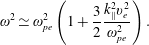


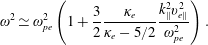


For the case of S waves:
-
(i) Isotropic Kappa distribution of type I:
(6.7)
$$\begin{eqnarray}\displaystyle \unicode[STIX]{x1D714}^{2}\left(1+2\frac{\unicode[STIX]{x1D705}_{e}-1/2}{\unicode[STIX]{x1D705}_{e}-3/2}\frac{\unicode[STIX]{x1D714}_{pe}^{2}}{k_{\Vert }^{2}v_{e}^{2}}\right)=\unicode[STIX]{x1D714}_{pi}^{2}. & & \displaystyle\end{eqnarray}$$
-
(ii) Isotropic Kappa distribution of type II:
(6.8)
$$\begin{eqnarray}\displaystyle \unicode[STIX]{x1D714}^{2}\left(1+2\frac{\unicode[STIX]{x1D705}_{e}-3/2}{\unicode[STIX]{x1D705}_{e}}\frac{\unicode[STIX]{x1D714}_{pe}^{2}}{k_{\Vert }^{2}v_{e}^{2}}\right)=\unicode[STIX]{x1D714}_{pi}^{2}. & & \displaystyle\end{eqnarray}$$
-
(iii) Bi-Kappa distribution of type I:
(6.9)
$$\begin{eqnarray}\displaystyle \unicode[STIX]{x1D714}^{2}\left(1+2\frac{\unicode[STIX]{x1D705}_{e}-1/2}{\unicode[STIX]{x1D705}_{e}-3/2}\frac{\unicode[STIX]{x1D714}_{pe}^{2}}{k_{\Vert }^{2}v_{e\Vert }^{2}}\right)=\unicode[STIX]{x1D714}_{pi}^{2}. & & \displaystyle\end{eqnarray}$$
-
(iv) Bi-Kappa distribution of type II:
(6.10)
$$\begin{eqnarray}\displaystyle \unicode[STIX]{x1D714}^{2}\left(1+2\frac{\unicode[STIX]{x1D705}_{e}-3/2}{\unicode[STIX]{x1D705}_{e}}\frac{\unicode[STIX]{x1D714}_{pe}^{2}}{k_{\Vert }^{2}v_{e\Vert }^{2}}\right)=\unicode[STIX]{x1D714}_{pi}^{2}. & & \displaystyle\end{eqnarray}$$
-
(v) Product-bi-Kappa distribution of type I:
(6.11)
$$\begin{eqnarray}\displaystyle \unicode[STIX]{x1D714}^{2}\left(1+2\frac{\unicode[STIX]{x1D705}_{e\Vert }+1/2}{\unicode[STIX]{x1D705}_{e\Vert }-1/2}\frac{\unicode[STIX]{x1D714}_{pe}^{2}}{k_{\Vert }^{2}v_{e\Vert }^{2}}\right)=\unicode[STIX]{x1D714}_{pi}^{2}. & & \displaystyle\end{eqnarray}$$
-
(vi) Product-bi-Kappa distribution of type II:
(6.12)
$$\begin{eqnarray}\displaystyle \unicode[STIX]{x1D714}^{2}\left(1+2\frac{\unicode[STIX]{x1D705}_{e\Vert }-1/2}{\unicode[STIX]{x1D705}_{e\Vert }}\frac{\unicode[STIX]{x1D714}_{pe}^{2}}{k_{\Vert }^{2}v_{e\Vert }^{2}}\right)=\unicode[STIX]{x1D714}_{pi}^{2}. & & \displaystyle\end{eqnarray}$$

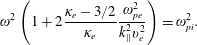

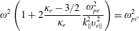


It is seen that, given the temperature parameter
 $T_{\unicode[STIX]{x1D6FD}}$
, distributions of type I, either isotropic or anisotropic, lead to the same form of the dispersion relation for Langmuir waves as the Maxwellian or bi-Maxwellian distributions. Dispersion relations for L waves obtained with distributions of type II feature a dependence on wavenumber which is dependent on
 $\unicode[STIX]{x1D705}_{\unicode[STIX]{x1D6FD}}$
(or
 $\unicode[STIX]{x1D705}_{\unicode[STIX]{x1D6FD}\Vert }$
), and it is seen that the difference relative to the Maxwellian case increases for small values of
 $\unicode[STIX]{x1D705}$
.
In the case of S waves, it is seen that both forms of Kappa distributions which have been considered, type I and type II, lead to dispersion relations which are different from those obtained in the case of Maxwellian or bi-Maxwellian plasmas.
The second approach to the presentation of the results obtained is by emphasis on the averaged squared velocity instead of the
 $T$
parameter. This second approach seems indicated for comparison with experimental data or with data generated in PIC simulations, since the average squared velocity of the particles can be directly obtained from the observations or from the numerical data generated in the simulations. In terms of the average value of the squared velocity, the dispersion relation which we have obtained can be written as follows.
For the case of L waves:
-
(i) Isotropic Kappa distribution of type I:
(6.13)
$$\begin{eqnarray}\displaystyle \unicode[STIX]{x1D714}^{2}\simeq \unicode[STIX]{x1D714}_{pe}^{2}\left(1+3\frac{k_{\Vert }^{2}\langle v_{\Vert }^{2}\rangle _{e}}{\unicode[STIX]{x1D714}_{pe}^{2}}\right). & & \displaystyle\end{eqnarray}$$
-
(ii) Isotropic Kappa distribution of type II:
(6.14)
$$\begin{eqnarray}\displaystyle \unicode[STIX]{x1D714}^{2}\simeq \unicode[STIX]{x1D714}_{pe}^{2}\left(1+3\frac{k_{\Vert }^{2}\langle v_{\Vert }^{2}\rangle _{e}}{\unicode[STIX]{x1D714}_{pe}^{2}}\right). & & \displaystyle\end{eqnarray}$$
-
(iii) Bi-Kappa distribution of type I:
(6.15)
$$\begin{eqnarray}\displaystyle \unicode[STIX]{x1D714}^{2}\simeq \unicode[STIX]{x1D714}_{pe}^{2}\left(1+3\frac{k_{\Vert }^{2}\langle v_{\Vert }^{2}\rangle _{e}}{\unicode[STIX]{x1D714}_{pe}^{2}}\right). & & \displaystyle\end{eqnarray}$$
-
(iv) Bi-Kappa distribution of type II:
(6.16)
$$\begin{eqnarray}\displaystyle \unicode[STIX]{x1D714}^{2}\simeq \unicode[STIX]{x1D714}_{pe}^{2}\left(1+3\frac{k_{\Vert }^{2}\langle v_{\Vert }^{2}\rangle _{e}}{\unicode[STIX]{x1D714}_{pe}^{2}}\right). & & \displaystyle\end{eqnarray}$$
-
(v) Product-bi-Kappa distribution of type I:
(6.17)
$$\begin{eqnarray}\displaystyle \unicode[STIX]{x1D714}^{2}\simeq \unicode[STIX]{x1D714}_{pe}^{2}\left(1+3\frac{k_{\Vert }^{2}\langle v_{\Vert }^{2}\rangle _{e}}{\unicode[STIX]{x1D714}_{pe}^{2}}\right). & & \displaystyle\end{eqnarray}$$
-
(vi) Product-bi-Kappa distribution of type II:
(6.18)
$$\begin{eqnarray}\displaystyle \unicode[STIX]{x1D714}^{2}\simeq \unicode[STIX]{x1D714}_{pe}^{2}\left(1+3\frac{k_{\Vert }^{2}\langle v_{\Vert }^{2}\rangle _{e}}{\unicode[STIX]{x1D714}_{pe}^{2}}\right). & & \displaystyle\end{eqnarray}$$
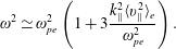
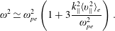

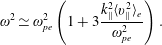
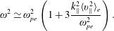
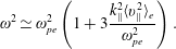
For the case of S waves:
-
(i) Isotropic Kappa distribution of type I:
(6.19)
$$\begin{eqnarray}\displaystyle \unicode[STIX]{x1D714}^{2}\left(1+\frac{\unicode[STIX]{x1D705}_{e}-1/2}{\unicode[STIX]{x1D705}_{e}-3/2}\frac{\unicode[STIX]{x1D714}_{pe}^{2}}{k_{\Vert }^{2}\langle v_{\Vert }^{2}\rangle _{e}}\right)=\unicode[STIX]{x1D714}_{pi}^{2}. & & \displaystyle\end{eqnarray}$$
-
(ii) Isotropic Kappa distribution of type II:
(6.20)
$$\begin{eqnarray}\displaystyle \unicode[STIX]{x1D714}^{2}\left(1+\frac{\unicode[STIX]{x1D705}_{e}-3/2}{\unicode[STIX]{x1D705}_{e}-5/2}\frac{\unicode[STIX]{x1D714}_{pe}^{2}}{k_{\Vert }^{2}\langle v_{\Vert }^{2}\rangle _{e}}\right)=\unicode[STIX]{x1D714}_{pi}^{2}. & & \displaystyle\end{eqnarray}$$
-
(iii) Bi-Kappa distribution of type I:
(6.21)
$$\begin{eqnarray}\displaystyle \unicode[STIX]{x1D714}^{2}\left(1+\frac{\unicode[STIX]{x1D705}_{e}-1/2}{\unicode[STIX]{x1D705}_{e}-3/2}\frac{\unicode[STIX]{x1D714}_{pe}^{2}}{k_{\Vert }^{2}\langle v_{\Vert }^{2}\rangle _{e}}\right)=\unicode[STIX]{x1D714}_{pi}^{2}. & & \displaystyle\end{eqnarray}$$
-
(iv) Bi-Kappa distribution of type II:
(6.22)
$$\begin{eqnarray}\displaystyle \unicode[STIX]{x1D714}^{2}\left(1+\frac{\unicode[STIX]{x1D705}_{e}-3/2}{\unicode[STIX]{x1D705}_{e}-5/2}\frac{\unicode[STIX]{x1D714}_{pe}^{2}}{k_{\Vert }^{2}\langle v_{\Vert }^{2}\rangle _{e}}\right)=\unicode[STIX]{x1D714}_{pi}^{2}. & & \displaystyle\end{eqnarray}$$
-
(v) Product-bi-Kappa distribution of type I:
(6.23)
$$\begin{eqnarray}\displaystyle \unicode[STIX]{x1D714}^{2}\left(1+\frac{\unicode[STIX]{x1D705}_{e\Vert }+1/2}{\unicode[STIX]{x1D705}_{e\Vert }-1/2}\frac{\unicode[STIX]{x1D714}_{pe}^{2}}{k_{\Vert }^{2}\langle v_{\Vert }^{2}\rangle _{e}}\right)=\unicode[STIX]{x1D714}_{pi}^{2}. & & \displaystyle\end{eqnarray}$$
-
(vi) Product-bi-Kappa distribution of type II:
(6.24)
$$\begin{eqnarray}\displaystyle \unicode[STIX]{x1D714}^{2}\left(1+\frac{\unicode[STIX]{x1D705}_{e\Vert }-1/2}{\unicode[STIX]{x1D705}_{e\Vert }-3/2}\frac{\unicode[STIX]{x1D714}_{pe}^{2}}{k_{\Vert }^{2}\langle v_{\Vert }^{2}\rangle _{e}}\right)=\unicode[STIX]{x1D714}_{pi}^{2}. & & \displaystyle\end{eqnarray}$$


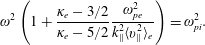

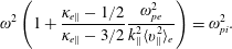
Both for L waves and for S waves, we have taken into account that for isotropic distributions
 $\langle v^{2}\rangle =3\langle v_{\Vert }^{2}\rangle$
.
According to this second approach, it is seen that both distributions of type I and type II lead to behaviour of the dispersion relation for L waves which is similar to that obtained in the Maxwellian case, with the dependence on wavenumber proportional to the average kinetic energy along parallel direction, without explicit dependence on the
 $\unicode[STIX]{x1D705}$
indexes. On the other hand, the dispersion relation for S waves exhibits dependence of the
 $\unicode[STIX]{x1D705}$
indexes both for type I and type II distributions, in the isotropic as well as in the anisotropic case. It is noticed that isotropic Kappa distributions and bi-Kappa distributions of a given type lead to the same form of dispersion relation, but the dispersion relations obtained for type I distributions are different from those obtained for type II distributions. However, the product-bi-Kappa distributions which we have utilized lead to the dispersion relations for S waves which are different for type I and type II distributions, and also different from the dispersion relations obtained for isotropic Kappa or bi-Kappa distributions.
In addition to these findings, which can be observed from the approximated analytical expressions, numerical analysis have shown that the actual and exact numerical solutions of the dispersion relation for L waves show significant difference relative to the approximate analytical solution, and that this difference increases with the decrease of the kappa indexes. Moreover, the numerical results obtained have shown that the dispersion relations for L waves are significantly different, for two different representations of the Kappa distributions which are pervasively used in the literature in recent years.
The dispersion relations for S waves also are significantly different, for the two representations of Kappa distributions which have been considered in the analysis. For the S waves there is also significant difference between the results obtained with the approximate analytical solution and with the exact dispersion relation. However, contrary to what is observed for L waves, the difference between the exact and the expanded dispersion relation for S waves decreases with the decrease of
 $\unicode[STIX]{x1D705}$
.
Acknowledgements
L.F.Z. acknowledges support from CNPq (Brazil), grant no. 304363/2014-6. R.G. acknowledges support from CNPq (Brazil), grants no. 478728/2012-3 and 307626/2015-6. F.J.R.S. acknowledges support from CNPq (Brazil), grant no. 473931/2013-3.
Appendix A. Evaluation of the integrals
$J(n,m,h;f_{\unicode[STIX]{x1D6FD}})$
and
$I$
in the case of Kappa distribution functions


Here we present details of the evaluation of the integrals which appear in the components of the dispersion relation, for the case in which the distribution functions of plasma particles are given by (2.1). We consider the generic case of a magnetized plasma, and write (1.2) in terms of dimensionless variables,
 $$\begin{eqnarray}\displaystyle J(n,m,h;f_{\unicode[STIX]{x1D6FD}})=z\int \,\text{d}^{3}u\,\frac{u_{\Vert }^{h}u_{\bot }^{2(m-1)}u_{\bot }L(f_{\unicode[STIX]{x1D6FD}})}{z-nr_{\unicode[STIX]{x1D6FD}}-q_{\Vert }u_{\Vert }}, & & \displaystyle\end{eqnarray}$$
where the distribution function is also written in terms of dimensionless variables, normalized such that
 $\int \,\text{d}^{3}u\,f_{\unicode[STIX]{x1D6FD}}=1$
. For simplicity of notation, here we will write
 $\unicode[STIX]{x1D705}$
and
 $\unicode[STIX]{x1D6FC}$
instead of
 $\unicode[STIX]{x1D705}_{\unicode[STIX]{x1D6FD}}$
and
 $\unicode[STIX]{x1D6FC}_{\unicode[STIX]{x1D6FD}}$
.
Using the differential operators,
 $$\begin{eqnarray}\displaystyle {\mathcal{L}}(f_{\unicode[STIX]{x1D6FD}}) & = & \displaystyle \displaystyle \left(u_{\Vert }\frac{\unicode[STIX]{x2202}}{\unicode[STIX]{x2202}u_{\bot }}-u_{\bot }\frac{\unicode[STIX]{x2202}}{\unicode[STIX]{x2202}u_{\Vert }}\right)f_{\unicode[STIX]{x1D6FD}}=0,\end{eqnarray}$$
 $$\begin{eqnarray}\displaystyle L(f_{\unicode[STIX]{x1D6FD}}) & = & \displaystyle \displaystyle \left[\left(1-\frac{q_{\Vert }}{z}u_{\Vert }\right)\frac{\unicode[STIX]{x2202}}{\unicode[STIX]{x2202}u_{\bot }}+\frac{q_{\Vert }}{z}u_{\bot }\frac{\unicode[STIX]{x2202}}{\unicode[STIX]{x2202}u_{\Vert }}\right]f_{\unicode[STIX]{x1D6FD}}\nonumber\\ \displaystyle & = & \displaystyle \displaystyle -\left[\left(1-\frac{q_{\Vert }}{z}u_{\Vert }\right)\frac{\unicode[STIX]{x1D705}+\unicode[STIX]{x1D6FC}}{\unicode[STIX]{x1D705}}\frac{2u_{\bot }}{u_{\unicode[STIX]{x1D6FD},\unicode[STIX]{x1D705}}^{2}}\left(1+\frac{u^{2}}{\unicode[STIX]{x1D705}u_{\unicode[STIX]{x1D6FD},\unicode[STIX]{x1D705}}^{2}}\right)^{-1}\right.\nonumber\\ \displaystyle & & \displaystyle \left.+\,\frac{q_{\Vert }}{z}u_{\bot }\frac{\unicode[STIX]{x1D705}+\unicode[STIX]{x1D6FC}}{\unicode[STIX]{x1D705}}\frac{2u_{\Vert }}{u_{\unicode[STIX]{x1D6FD},\unicode[STIX]{x1D705}}^{2}}\left(1+\frac{u^{2}}{\unicode[STIX]{x1D705}u_{\unicode[STIX]{x1D6FD},\unicode[STIX]{x1D705}}^{2}}\right)^{-1}\right]f_{\unicode[STIX]{x1D6FD}},\end{eqnarray}$$
which leads to
 $$\begin{eqnarray}L(f_{\unicode[STIX]{x1D6FD}})=-\frac{2u_{\bot }}{u_{\unicode[STIX]{x1D6FD},\unicode[STIX]{x1D705}}^{2}}\frac{\unicode[STIX]{x1D705}+\unicode[STIX]{x1D6FC}}{\unicode[STIX]{x1D705}}\left(1+\frac{u^{2}}{\unicode[STIX]{x1D705}u_{\unicode[STIX]{x1D6FD},\unicode[STIX]{x1D705}}^{2}}\right)^{-1}f_{\unicode[STIX]{x1D6FD}}.\end{eqnarray}$$
Therefore, the integral containing operator
 ${\mathcal{L}}$
vanishes, and the expression for the
 $J(n,m,h;f_{\unicode[STIX]{x1D6FD}})$
becomes
 $$\begin{eqnarray}\displaystyle \frac{2\unicode[STIX]{x1D714}}{u_{\unicode[STIX]{x1D6FD},\unicode[STIX]{x1D705}}^{2}v_{\ast }k_{\Vert }}\frac{(2\unicode[STIX]{x03C0})n_{\unicode[STIX]{x1D6FD}0}}{\unicode[STIX]{x03C0}^{3/2}\unicode[STIX]{x1D705}^{3/2}u_{\unicode[STIX]{x1D6FD},\unicode[STIX]{x1D705}}^{3}}\frac{\unicode[STIX]{x1D705}+\unicode[STIX]{x1D6FC}}{\unicode[STIX]{x1D705}}\frac{\unicode[STIX]{x1D6E4}(\unicode[STIX]{x1D705}+\unicode[STIX]{x1D6FC})}{\unicode[STIX]{x1D6E4}(\unicode[STIX]{x1D705}+\unicode[STIX]{x1D6FC}-3/2)}\int _{0}^{\infty }\,\text{d}u_{\bot }\,u_{\bot }^{2m+1} & & \displaystyle \nonumber\\ \displaystyle \times \int _{-\infty }^{\infty }\,\text{d}u_{\Vert }\,\frac{u_{\Vert }^{h}}{u_{\Vert }-u_{\Vert ,res}}\left(1+\frac{u_{\Vert }^{2}}{\unicode[STIX]{x1D705}u_{\unicode[STIX]{x1D6FD},\unicode[STIX]{x1D705}}^{2}}+\frac{u_{\bot }^{2}}{\unicode[STIX]{x1D705}u_{\unicode[STIX]{x1D6FD},\unicode[STIX]{x1D705}}^{2}}\right)^{-(\unicode[STIX]{x1D705}+\unicode[STIX]{x1D6FC}+1)}, & & \displaystyle\end{eqnarray}$$
where
 $u_{\Vert ,res}=(\unicode[STIX]{x1D714}-n\unicode[STIX]{x1D6FA}_{\unicode[STIX]{x1D6FD}})/(k_{\Vert }v_{\ast })$
.
By defining
 $\unicode[STIX]{x1D6FC}_{\Vert }=1+u_{\Vert }^{2}/(\unicode[STIX]{x1D705}u_{\unicode[STIX]{x1D6FD},\unicode[STIX]{x1D705}}^{2})$
, we can write this expression as follows,
 $$\begin{eqnarray}\displaystyle & & \displaystyle \displaystyle \frac{2\unicode[STIX]{x1D714}}{u_{\unicode[STIX]{x1D6FD},\unicode[STIX]{x1D705}}^{2}v_{\ast }k_{\Vert }}\frac{(2\unicode[STIX]{x03C0})n_{\unicode[STIX]{x1D6FD}0}}{\unicode[STIX]{x03C0}^{3/2}\unicode[STIX]{x1D705}^{3/2}u_{\unicode[STIX]{x1D6FD},\unicode[STIX]{x1D705}}^{3}}\frac{\unicode[STIX]{x1D705}+\unicode[STIX]{x1D6FC}}{\unicode[STIX]{x1D705}}\frac{\unicode[STIX]{x1D6E4}(\unicode[STIX]{x1D705}+\unicode[STIX]{x1D6FC})}{\unicode[STIX]{x1D6E4}(\unicode[STIX]{x1D705}+\unicode[STIX]{x1D6FC}-3/2)}\nonumber\\ \displaystyle & & \displaystyle \quad \times \int _{-\infty }^{\infty }\,\text{d}u_{\Vert }\,\frac{u_{\Vert }^{h}}{u_{\Vert }-u_{\Vert ,res}}\left(1+\frac{u_{\Vert }^{2}}{\unicode[STIX]{x1D6FC}_{\Vert }\unicode[STIX]{x1D705}u_{\unicode[STIX]{x1D6FD},\unicode[STIX]{x1D705}}^{2}}\right)^{-(\unicode[STIX]{x1D705}+\unicode[STIX]{x1D6FC}+1)}\nonumber\\ \displaystyle & & \displaystyle \quad \times \int _{0}^{\infty }\,\text{d}u_{\bot }\,u_{\bot }^{2m+1}\left(1+\frac{u_{\bot }^{2}}{\unicode[STIX]{x1D6FC}_{\Vert }\unicode[STIX]{x1D705}u_{\unicode[STIX]{x1D6FD},\unicode[STIX]{x1D705}}^{2}}\right)^{-(\unicode[STIX]{x1D705}+\unicode[STIX]{x1D6FC}+1)}.\end{eqnarray}$$
Changing variable in the integrals over
 $u_{\bot }$
,
 $t=u_{\bot }^{2}/(\unicode[STIX]{x1D6FC}_{\Vert }\unicode[STIX]{x1D705}u_{\unicode[STIX]{x1D6FD},\unicode[STIX]{x1D705}}^{2})$
, the integral over
 $u_{\bot }$
becomes
 $$\begin{eqnarray}\displaystyle \frac{1}{2}\unicode[STIX]{x1D6FC}_{\Vert }^{m+1}\unicode[STIX]{x1D705}^{m+1}u_{\unicode[STIX]{x1D6FD},\unicode[STIX]{x1D705}}^{2(m+1)}\int _{0}^{\infty }\,\text{d}t\frac{t^{m}}{(1+t)^{\unicode[STIX]{x1D705}+\unicode[STIX]{x1D6FC}+1}}. & & \displaystyle\end{eqnarray}$$
It is seen that we can use the following integral, with appropriate values of
 $z$
and
 $w$
,
 $$\begin{eqnarray}\int _{0}^{\infty }\,\text{d}t\frac{t^{z-1}}{(1+t)^{w+z}}=\frac{\unicode[STIX]{x1D6E4}(z)\unicode[STIX]{x1D6E4}(w)}{\unicode[STIX]{x1D6E4}(w+z)},\quad (\text{Re}\,z>0,\text{Re}\,w>0),\end{eqnarray}$$
which leads to the following for the
 $u_{\bot }$
integral,
 $$\begin{eqnarray}\displaystyle \frac{1}{2}\unicode[STIX]{x1D6FC}_{\Vert }^{m+1}\unicode[STIX]{x1D705}^{m+1}u_{\unicode[STIX]{x1D6FD},\unicode[STIX]{x1D705}}^{2(m+1)}\frac{\unicode[STIX]{x1D6E4}(m+1)\unicode[STIX]{x1D6E4}(\unicode[STIX]{x1D705}+\unicode[STIX]{x1D6FC}-m)}{\unicode[STIX]{x1D6E4}(\unicode[STIX]{x1D705}+\unicode[STIX]{x1D6FC}+1)}. & & \displaystyle\end{eqnarray}$$
Using this result,
 $$\begin{eqnarray}\displaystyle J(n,m,h;f_{\unicode[STIX]{x1D6FD}}) & = & \displaystyle \displaystyle \frac{z}{q_{\Vert }}\frac{(2\unicode[STIX]{x03C0})n_{\unicode[STIX]{x1D6FD}0}}{\unicode[STIX]{x03C0}^{3/2}}\unicode[STIX]{x1D705}^{m-3/2}u_{\unicode[STIX]{x1D6FD},\unicode[STIX]{x1D705}}^{2m-3+h}(m!)\nonumber\\ \displaystyle & & \displaystyle \displaystyle \times \,\frac{\unicode[STIX]{x1D6E4}(\unicode[STIX]{x1D705}+\unicode[STIX]{x1D6FC}-m)}{\unicode[STIX]{x1D6E4}(\unicode[STIX]{x1D705}+\unicode[STIX]{x1D6FC}-3/2)}\int _{-\infty }^{\infty }\,\text{d}s\,\frac{s^{h}}{s-\unicode[STIX]{x1D701}_{\unicode[STIX]{x1D6FD}}^{n}}\left(1+\frac{s^{2}}{\unicode[STIX]{x1D705}}\right)^{m-\unicode[STIX]{x1D705}-\unicode[STIX]{x1D6FC}},\end{eqnarray}$$
where
 $s=u_{\Vert }/u_{\unicode[STIX]{x1D6FD},\unicode[STIX]{x1D705}}$
and
 $\unicode[STIX]{x1D701}_{\unicode[STIX]{x1D6FD}}^{n}=(z-nr_{\unicode[STIX]{x1D6FD}})/(q_{\Vert }u_{\unicode[STIX]{x1D6FD},\unicode[STIX]{x1D705}})$
.
We now introduce the plasma dispersion function of order
 $m$
, for Kappa distributions,
 $$\begin{eqnarray}\displaystyle Z_{\unicode[STIX]{x1D705}}^{(m)}(\unicode[STIX]{x1D709})=\frac{1}{\unicode[STIX]{x03C0}^{1/2}}\frac{\unicode[STIX]{x1D6E4}(\unicode[STIX]{x1D705})}{\unicode[STIX]{x1D705}^{1/2}\unicode[STIX]{x1D6E4}(\unicode[STIX]{x1D705}-1/2)}\int _{-\infty }^{\infty }\frac{\text{d}s}{(s-\unicode[STIX]{x1D709})(1+s^{2}/\unicode[STIX]{x1D705})^{\unicode[STIX]{x1D705}+m}}, & & \displaystyle\end{eqnarray}$$
which can be written in terms of the Gauss hypergeometric function
 $_{2}F_{1}(a,b,c,z)$
, as in (2.3), for
 $\unicode[STIX]{x1D705}>-m-1/2$
.
Let us now consider in some detail the evaluation of
 $J(n,m,h;f_{\unicode[STIX]{x1D6FD}})$
in the case of
 $h=0$
,
 $$\begin{eqnarray}\displaystyle J(n,m,0;f_{\unicode[STIX]{x1D6FD}}) & = & \displaystyle \displaystyle \frac{z}{q_{\Vert }}\frac{(2\unicode[STIX]{x03C0})n_{\unicode[STIX]{x1D6FD}0}}{\unicode[STIX]{x03C0}^{3/2}}\unicode[STIX]{x1D705}^{m-3/2}u_{\unicode[STIX]{x1D6FD},\unicode[STIX]{x1D705}}^{2m-3}(m!)\nonumber\\ \displaystyle & & \displaystyle \displaystyle \times \,\frac{\unicode[STIX]{x1D6E4}(\unicode[STIX]{x1D705}+\unicode[STIX]{x1D6FC}-m)}{\unicode[STIX]{x1D6E4}(\unicode[STIX]{x1D705}+\unicode[STIX]{x1D6FC}-3/2)}\int _{-\infty }^{\infty }\,\text{d}s\frac{1}{s-\unicode[STIX]{x1D701}_{\unicode[STIX]{x1D6FD}}^{n}}\left(1+\frac{s^{2}}{\unicode[STIX]{x1D705}}\right)^{-(\unicode[STIX]{x1D705}+\unicode[STIX]{x1D6FC}-m)}.\end{eqnarray}$$
The integrand diverges for
 $\unicode[STIX]{x1D705}+1-m<0$
. For
 $m<\unicode[STIX]{x1D705}+1$
, the integral can be evaluated using (A 11) and (2.3), leading to
 $$\begin{eqnarray}\displaystyle J(n,m,0;f_{\unicode[STIX]{x1D6FD}}) & = & \displaystyle (2)n_{\unicode[STIX]{x1D6FD}0}(\unicode[STIX]{x1D705}u_{\unicode[STIX]{x1D6FD},\unicode[STIX]{x1D705}}^{2})^{m-1}(u_{\unicode[STIX]{x1D6FD},\unicode[STIX]{x1D705}})^{0}(m!)\nonumber\\ \displaystyle & & \displaystyle \displaystyle \times \,\frac{\unicode[STIX]{x1D6E4}(\unicode[STIX]{x1D705}+\unicode[STIX]{x1D6FC}-m)\unicode[STIX]{x1D6E4}(\unicode[STIX]{x1D705}-1/2)}{\unicode[STIX]{x1D6E4}(\unicode[STIX]{x1D705}+\unicode[STIX]{x1D6FC}-3/2)\unicode[STIX]{x1D6E4}(\unicode[STIX]{x1D705})}\unicode[STIX]{x1D701}_{\unicode[STIX]{x1D6FD}}^{0}Z_{\unicode[STIX]{x1D705}}^{(\unicode[STIX]{x1D6FC}-m)}(\unicode[STIX]{x1D701}_{\unicode[STIX]{x1D6FD}}^{n}),\end{eqnarray}$$
where
 $\unicode[STIX]{x1D701}_{\unicode[STIX]{x1D6FD}}^{0}=z/(q_{\Vert }u_{\unicode[STIX]{x1D6FD},\unicode[STIX]{x1D705}})$
and
 $\unicode[STIX]{x1D701}_{\unicode[STIX]{x1D6FD}}^{n}=(z-nr_{\unicode[STIX]{x1D6FD}})/(q_{\Vert }u_{\unicode[STIX]{x1D6FD},\unicode[STIX]{x1D705}})$
.
For other values of
 $h$
the evaluation is similar. For instance, for the cases of
 $h=1$
and
 $h=2$
, one obtains
 $$\begin{eqnarray}\displaystyle & & \displaystyle \displaystyle J(n,m,1;f_{\unicode[STIX]{x1D6FD}})\nonumber\\ \displaystyle & & \displaystyle \quad =(2)n_{\unicode[STIX]{x1D6FD}0}(\unicode[STIX]{x1D705}u_{\unicode[STIX]{x1D6FD},\unicode[STIX]{x1D705}}^{2})^{m-1}u_{\unicode[STIX]{x1D6FD},\unicode[STIX]{x1D705}}(m!)\unicode[STIX]{x1D701}_{\unicode[STIX]{x1D6FD}}^{0}\frac{\unicode[STIX]{x1D6E4}(\unicode[STIX]{x1D705}+\unicode[STIX]{x1D6FC}-m)\unicode[STIX]{x1D6E4}(\unicode[STIX]{x1D705}-1/2)}{\unicode[STIX]{x1D6E4}(\unicode[STIX]{x1D705}+\unicode[STIX]{x1D6FC}-3/2)\unicode[STIX]{x1D6E4}(\unicode[STIX]{x1D705})}\nonumber\\ \displaystyle & & \displaystyle \qquad \times \,\left(\frac{\unicode[STIX]{x1D6E4}(\unicode[STIX]{x1D705})\unicode[STIX]{x1D6E4}(\unicode[STIX]{x1D705}+\unicode[STIX]{x1D6FC}-m-1/2)}{\unicode[STIX]{x1D6E4}(\unicode[STIX]{x1D705}-1/2)\unicode[STIX]{x1D6E4}(\unicode[STIX]{x1D705}+\unicode[STIX]{x1D6FC}-m)}+\unicode[STIX]{x1D701}_{\unicode[STIX]{x1D6FD}}^{n}Z_{\unicode[STIX]{x1D705}}^{(\unicode[STIX]{x1D6FC}-m)}(\unicode[STIX]{x1D701}_{\unicode[STIX]{x1D6FD}}^{n})\right),\end{eqnarray}$$
 $$\begin{eqnarray}\displaystyle & & \displaystyle J(n,m,2;f_{\unicode[STIX]{x1D6FD}})\nonumber\\ \displaystyle & & \displaystyle \displaystyle \quad =(2)n_{\unicode[STIX]{x1D6FD}0}(\unicode[STIX]{x1D705}u_{\unicode[STIX]{x1D6FD},\unicode[STIX]{x1D705}}^{2})^{m-1}u_{\unicode[STIX]{x1D6FD},\unicode[STIX]{x1D705}}^{2}(m!)\unicode[STIX]{x1D701}_{\unicode[STIX]{x1D6FD}}^{0}\unicode[STIX]{x1D701}_{\unicode[STIX]{x1D6FD}}^{n}\frac{\unicode[STIX]{x1D6E4}(\unicode[STIX]{x1D705}+\unicode[STIX]{x1D6FC}-m)\unicode[STIX]{x1D6E4}(\unicode[STIX]{x1D705}-1/2)}{\unicode[STIX]{x1D6E4}(\unicode[STIX]{x1D705}+\unicode[STIX]{x1D6FC}-3/2)\unicode[STIX]{x1D6E4}(\unicode[STIX]{x1D705})}\nonumber\\ \displaystyle & & \displaystyle \displaystyle \qquad \times \,\left(\frac{\unicode[STIX]{x1D6E4}(\unicode[STIX]{x1D705})\unicode[STIX]{x1D6E4}(\unicode[STIX]{x1D705}+\unicode[STIX]{x1D6FC}-m-1/2)}{\unicode[STIX]{x1D6E4}(\unicode[STIX]{x1D705}-1/2)\unicode[STIX]{x1D6E4}(\unicode[STIX]{x1D705}+\unicode[STIX]{x1D6FC}-m)}+\unicode[STIX]{x1D701}_{\unicode[STIX]{x1D6FD}}^{n}Z_{\unicode[STIX]{x1D705}}^{(\unicode[STIX]{x1D6FC}-m)}(\unicode[STIX]{x1D701}_{\unicode[STIX]{x1D6FD}}^{n})\right).\end{eqnarray}$$
We can obtain approximated expressions which are valid when
 $|\unicode[STIX]{x1D701}_{\unicode[STIX]{x1D6FD}}^{n}|\gg s$
in the region which is relevant for the integration. We proceed from the equation which appears before (A 11), and then expand the denominator, obtaining
 $$\begin{eqnarray}\displaystyle J(n,m,h;f_{\unicode[STIX]{x1D6FD}}) & = & \displaystyle -\frac{z}{q_{\Vert }}\frac{(2\unicode[STIX]{x03C0})n_{\unicode[STIX]{x1D6FD}0}}{\unicode[STIX]{x03C0}^{3/2}}\unicode[STIX]{x1D705}^{m-3/2}u_{\unicode[STIX]{x1D6FD},\unicode[STIX]{x1D705}}^{2m-3+h}(m!)\frac{\unicode[STIX]{x1D6E4}(\unicode[STIX]{x1D705}+\unicode[STIX]{x1D6FC}-m)}{\unicode[STIX]{x1D6E4}(\unicode[STIX]{x1D705}+\unicode[STIX]{x1D6FC}-3/2)}\frac{1}{\unicode[STIX]{x1D701}_{\unicode[STIX]{x1D6FD}}^{n}}\nonumber\\ \displaystyle & & \displaystyle \times \int _{-\infty }^{\infty }\,\text{d}s\,s^{h}\left(1+\frac{s}{\unicode[STIX]{x1D701}_{\unicode[STIX]{x1D6FD}}^{n}}+\frac{s^{2}}{(\unicode[STIX]{x1D701}_{\unicode[STIX]{x1D6FD}}^{n})^{2}}+\cdots \,\right)\left(1+\frac{s^{2}}{\unicode[STIX]{x1D705}}\right)^{m-\unicode[STIX]{x1D705}-\unicode[STIX]{x1D6FC}}.\end{eqnarray}$$
Neglecting terms of order
 $(s/\unicode[STIX]{x1D701})^{3}$
, taking into account the parity of the integrands and using (A 8) with
 $t=s^{2}/\unicode[STIX]{x1D705}$
, we obtain, for the cases
 $h=0$
,
 $h=1$
and
 $h=2$
,
 $$\begin{eqnarray}\displaystyle \displaystyle J(n,m,0;f_{\unicode[STIX]{x1D6FD}}) & = & \displaystyle -2n_{\unicode[STIX]{x1D6FD}0}\unicode[STIX]{x1D705}^{m-1}u_{\unicode[STIX]{x1D6FD},\unicode[STIX]{x1D705}}^{2m-2}(m!)\nonumber\\ \displaystyle & & \displaystyle \times \,\frac{\unicode[STIX]{x1D701}_{\unicode[STIX]{x1D6FD}}^{0}}{\unicode[STIX]{x1D701}_{\unicode[STIX]{x1D6FD}}^{n}}\frac{\unicode[STIX]{x1D6E4}(\unicode[STIX]{x1D705}+\unicode[STIX]{x1D6FC}-m-3/2)}{\unicode[STIX]{x1D6E4}(\unicode[STIX]{x1D705}+\unicode[STIX]{x1D6FC}-3/2)}\left(\unicode[STIX]{x1D705}+\unicode[STIX]{x1D6FC}-m-\frac{3}{2}+\frac{1}{(\unicode[STIX]{x1D701}_{\unicode[STIX]{x1D6FD}}^{n})^{2}}\frac{\unicode[STIX]{x1D705}}{2}\right),\end{eqnarray}$$
 $$\begin{eqnarray}\displaystyle \displaystyle J(n,m,1;f_{\unicode[STIX]{x1D6FD}}) & = & \displaystyle -n_{\unicode[STIX]{x1D6FD}0}\unicode[STIX]{x1D705}^{m}u_{\unicode[STIX]{x1D6FD},\unicode[STIX]{x1D705}}^{2m-1}(m!)\frac{\unicode[STIX]{x1D701}_{\unicode[STIX]{x1D6FD}}^{0}}{(\unicode[STIX]{x1D701}_{\unicode[STIX]{x1D6FD}}^{n})^{2}}\frac{\unicode[STIX]{x1D6E4}(\unicode[STIX]{x1D705}+\unicode[STIX]{x1D6FC}-m-3/2)}{\unicode[STIX]{x1D6E4}(\unicode[STIX]{x1D705}+\unicode[STIX]{x1D6FC}-3/2)},\end{eqnarray}$$
 $$\begin{eqnarray}\displaystyle J(n,m,2;f_{\unicode[STIX]{x1D6FD}}) & = & \displaystyle -n_{\unicode[STIX]{x1D6FD}0}\unicode[STIX]{x1D705}^{m}u_{\unicode[STIX]{x1D6FD},\unicode[STIX]{x1D705}}^{2m}(m!)\nonumber\\ \displaystyle & & \displaystyle \times \,\frac{\unicode[STIX]{x1D701}_{\unicode[STIX]{x1D6FD}}^{0}}{\unicode[STIX]{x1D701}_{\unicode[STIX]{x1D6FD}}^{n}}\frac{\unicode[STIX]{x1D6E4}(\unicode[STIX]{x1D705}+\unicode[STIX]{x1D6FC}-m-5/2)}{\unicode[STIX]{x1D6E4}(\unicode[STIX]{x1D705}+\unicode[STIX]{x1D6FC}-3/2)}\left(\unicode[STIX]{x1D705}+\unicode[STIX]{x1D6FC}-m-\frac{5}{2}+\frac{1}{(\unicode[STIX]{x1D701}_{\unicode[STIX]{x1D6FD}}^{n})^{2}}\frac{3\unicode[STIX]{x1D705}}{2}\right).\end{eqnarray}$$
An approximation valid for small values of
 $|\unicode[STIX]{x1D701}_{\unicode[STIX]{x1D6FD}}^{n}|$
can be obtained by the following expansion of the integrand in the expression which appears before (A 11)
 $$\begin{eqnarray}\displaystyle J(n,m,h;f_{\unicode[STIX]{x1D6FD}}) & = & \displaystyle \frac{z}{q_{\Vert }}\frac{(2\unicode[STIX]{x03C0})n_{\unicode[STIX]{x1D6FD}0}}{\unicode[STIX]{x03C0}^{3/2}}\unicode[STIX]{x1D705}^{m-3/2}u_{\unicode[STIX]{x1D6FD}}^{2m-3+h}(m!)\frac{\unicode[STIX]{x1D6E4}(\unicode[STIX]{x1D705}+\unicode[STIX]{x1D6FC}-m)}{\unicode[STIX]{x1D6E4}(\unicode[STIX]{x1D705}+\unicode[STIX]{x1D6FC}-3/2)}\nonumber\\ \displaystyle & & \displaystyle \times \int _{-\infty }^{\infty }\,\text{d}s\,s^{h-1}\left(1+\frac{s^{2}}{\unicode[STIX]{x1D705}}\right)^{m-\unicode[STIX]{x1D705}-\unicode[STIX]{x1D6FC}}\left(1+\frac{\hat{\unicode[STIX]{x1D701}}_{\unicode[STIX]{x1D6FD}}^{n}}{s}+\frac{(\hat{\unicode[STIX]{x1D701}}_{\unicode[STIX]{x1D6FD}}^{n})^{2}}{s^{2}}+\cdots \right).\end{eqnarray}$$
Neglecting terms of order
 $(\unicode[STIX]{x1D701}/s)^{3}$
, taking into account the parity of the integrands and using (A 8) with
 $t=s^{2}/\unicode[STIX]{x1D705}$
, we obtain, for the cases
 $h=0$
,
 $h=1$
and
 $h=2$
,
 $$\begin{eqnarray}\displaystyle J(n,m,0;f_{\unicode[STIX]{x1D6FD}}) & = & \displaystyle -(4)n_{\unicode[STIX]{x1D6FD}0}\unicode[STIX]{x1D705}^{m-2}u_{\unicode[STIX]{x1D6FD}}^{2m-2}(m!)\frac{\unicode[STIX]{x1D6E4}(\unicode[STIX]{x1D705}+\unicode[STIX]{x1D6FC}-m+1/2)}{\unicode[STIX]{x1D6E4}(\unicode[STIX]{x1D705}+\unicode[STIX]{x1D6FC}-3/2)}\unicode[STIX]{x1D701}_{\unicode[STIX]{x1D6FD}}^{0}\hat{\unicode[STIX]{x1D701}}_{\unicode[STIX]{x1D6FD}}^{n}\end{eqnarray}$$
 $$\begin{eqnarray}\displaystyle J(n,m,1;f_{\unicode[STIX]{x1D6FD}}) & = & \displaystyle \displaystyle (2)n_{\unicode[STIX]{x1D6FD}0}\unicode[STIX]{x1D705}^{m-1/2}u_{\unicode[STIX]{x1D6FD}}^{2m-1}(m!)\frac{\unicode[STIX]{x1D6E4}(\unicode[STIX]{x1D705}+\unicode[STIX]{x1D6FC}-m-1/2)}{\unicode[STIX]{x1D6E4}(\unicode[STIX]{x1D705}+\unicode[STIX]{x1D6FC}-3/2)}\nonumber\\ \displaystyle & & \displaystyle \times \,\unicode[STIX]{x1D701}_{\unicode[STIX]{x1D6FD}}^{0}\displaystyle \left[1-2(\hat{\unicode[STIX]{x1D701}}_{\unicode[STIX]{x1D6FD}}^{n})^{2}\frac{(\unicode[STIX]{x1D705}+\unicode[STIX]{x1D6FC}-m-1/2)}{\unicode[STIX]{x1D705}}\right]\end{eqnarray}$$
 $$\begin{eqnarray}\displaystyle J(n,m,2;f_{\unicode[STIX]{x1D6FD}}) & = & \displaystyle (2)n_{\unicode[STIX]{x1D6FD}0}\unicode[STIX]{x1D705}^{m-1}u_{\unicode[STIX]{x1D6FD}}^{2m}(m!)\frac{\unicode[STIX]{x1D6E4}(\unicode[STIX]{x1D705}+\unicode[STIX]{x1D6FC}-m-1/2)}{\unicode[STIX]{x1D6E4}(\unicode[STIX]{x1D705}+\unicode[STIX]{x1D6FC}-3/2)}\unicode[STIX]{x1D701}_{\unicode[STIX]{x1D6FD}}^{0}\hat{\unicode[STIX]{x1D701}}_{\unicode[STIX]{x1D6FD}}^{n}.\end{eqnarray}$$



