Implications
The heritability is the proportion of phenotypic variation in a population due to genetic and environmental variance among individuals. In a simulation study, we evaluated the potential of accurately estimating the heritability based on molecular SNP markers using a Bayesian approach. Different population structures were used to ensure that the models have the capabilities of becoming broadly applied. The results from this study are of value for traits that are difficult or expensive to measure.
Introduction
Estimation of genetic parameters requires large sample sizes and preferable information about relationship among individuals. For quantitative traits such as rare diseases, individual feed consumption or behavioural traits, it can be difficult to obtain a sufficient large sample size that fulfils the requirement for estimation of genetic parameters. Measurement of the traits can be time-consuming or may require expensive and/or special equipment. For instance, the measurement of fatty acids by gas chromatography in bovine milk is both a time-consuming and costly process (Rutten et al., Reference Rutten, Bovenhuis, Hettinga, van Valenberg and van Arendonk2009). In other species such as fish and wild species, the information of relationship is either not available or it can be difficult to keep track of (Schwartz et al., Reference Schwartz, Luikart and Waples2007; Wenne et al., Reference Wenne, Boudry, Hemmer-Hansen, Lubieniecki, Was and Kause2007). Molecular single-nucleotide polymorphism (SNP) markers can become useful as a solution for estimation of genetic parameters, when sample sizes for different reasons may be limited and pedigree information is unavailable.
SNPs have, in recent years, become widely used and become available for a number of animal species with different coverage across the genomes. Their applications in studies of parameter estimation, including heritability, have become common (Visscher et al., Reference Visscher, Medland, Ferreira, Morley, Zhu, Cornes, Montgomery and Martin2006). During the last decade, attempts to estimate genetic parameters based on marker information have been successfully carried out (Thomas et al., Reference Thomas, Pemberton and Hill2000; Visscher et al., Reference Visscher, Hill and Wray2008). This has, for instance, been carried out in the studying of height of humans (Visscher et al., Reference Visscher, Medland, Ferreira, Morley, Zhu, Cornes, Montgomery and Martin2006; Makowsky et al., Reference Makowsky, Pajewski, Klimentidis, Vazquez, Duarte, Allison and de los Campos2011). The estimation precision with SNP markers is dependent on both the structure and size of the dataset. Cost reduction for obtaining precise estimates based on genomic information can be facilitated through careful consideration of dataset structure (Goddard et al., Reference Goddard, Hayes and Meuwissen2010; Pribyl et al., Reference Pribyl, Rehout, Citek and Pribylova2010).
Precision of heritability estimation using SNP markers is affected by a number of factors, such as sample size. Phenotypic measurement can, for instance, either be carried out directly on individuals, but may also be carried out indirectly on relatives. This is the case, for example, for female fertility for bulls, which require multiple observations to achieve an accurate breeding value for the sire (Mrode and Thompson, Reference Mrode and Thompson2005). Population structure, including the effective population size (N e), is another factor to take into account. The number of the samples needed for heritability estimation decreases in connection with lower N e. For traits that are only available in low numbers, this means that estimation of the heritability is easier to perform based on populations that have a low N e (Goddard et al., Reference Goddard, Hayes and Meuwissen2010). This is, for instance, useful in domesticated animals such as cattle populations, because N e is known to be low in these populations. This is the opposite for human populations, where N e is known to be high (Goddard and Hayes, Reference Goddard and Hayes2009). Increasing density of SNPs is known to increase the precision of heritability estimates; however, there are indications showing that there is a diminishing effect of increasing SNP density, a further increase in SNP density will only increase precision marginally (Goddard and Hayes, Reference Goddard and Hayes2009).
Previous studies have estimated heritability on a real dataset using restricted maximum likelihood (REML) with genomic relationship matrices (Veerkamp et al., Reference Veerkamp, Mulder, Thompson and Calus2011). Bayesian genomic models such as Bayes A and Bayes C were proposed for prediction, but have not yet been considered for estimation of SNP-explained variances. We utilize close variations of the Bayes A and Bayes C methods with extensions to estimate hyperparameters from the data. The aim of this work is to validate by simulation whether such Bayesian models are capable of estimating SNP-explained variances. In the present study, we simulated a number of different set-ups with the purpose of estimating heritability without pedigree information. Our objective was to evaluate (1) the possibility to estimate heritability in populations consisting of a limited number of individuals and with or without family structure; (2) how effective population size and density of SNPs affected the estimation; and (3) how sample size and size of heritability affected the precision of the estimation.
Material and methods
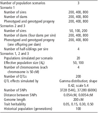
We investigated the potential to estimate heritability using SNPs, based on three different population scenarios. All scenarios were simulated with the following parameters: two densities of SNPs, four heritabilities, two N e and three sample sizes. Altogether, this yields 48 possible combinations within each of the three scenarios. Table 1 provides information about value(s) assigned to each variable.
Simulation parameters

QTL = quantitative trait loci; SNP = single-nucleotide polymorphism.
Each population scenario was simulated with the maximum of possible combinations of the parameters listed below, that is, 48 different set-ups for each population scenarios.
After populations were simulated, two Bayesian genomic prediction models were separately used to estimate heritability on each population within each of the three scenarios. For each population, we obtained two heritability estimates, one estimate from each model. In this way, it was possible for us to evaluate how each parameter affected the heritability estimate and its precision. From each population set-up, we also selected one replicate and estimated the heritability using a genomic relationship matrix and a REML approach. This estimate was compared with the estimates obtained with the two Bayesian models. In this way, we were able to validate whether the two Bayesian models obtained as good estimates as the more traditional REML approach.
Selection of animals
Selection of the animals that were used for phenotyping and genotyping was carried out in the following way: in scenario 1, an equal number of males and females were randomly selected to produce one daughter each for the next generation. This was carried out for 100 generations. At generation 101, one daughter was selected per sire, which was used for estimation of heritability. In scenario 2, animals were selected similar to scenario 1 but with a ratio of males and females of 1 : 4, that is, one male was crossed to four non-related females, yielding four half-siblings. In scenario 3, an equal number of sires and dams were selected as founders for generation 101. From generation 101, sires and dams were selected in the proportion of 1 : 4. Each sire–dam combination was set to produce two offspring to the next generation. This was repeated for nine generations. In generation 110, one daughter was selected from each sire–dam combination for heritability estimation. From generation 101 to 110, inbreeding was minimized. For all scenarios, individuals were simulated with a single trait with a heritability of either 0.05, 0.15, 0.30 or 0.50. In each scenario, the number of phenotyped animals, that is, number of progeny, was either 200, 400 or 800. These values will be used further on when referring to the different sample sizes in this paper.
Simulation of SNPs and quantitative trait loci (QTL)
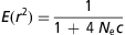
The number of chromosomes was four, with a total genome length of 200–50 cM for each chromosome. This length corresponds to ∼1/16 of the bovine genome. The bovine genome was used as a reference for calculation of the SNP density, that is, the distance between each pair of SNPs resembles the expected distance between a pair of SNPs from a 54k to 600k bovine SNP array. The bovine genome comprises 29 pairs of autosomes and one pair of sex chromosomes. The total length of the genome is estimated to be 3160 cM (Ihara et al., Reference Ihara, Takasuga, Mizoshita, Takeda, Sugimoto, Mizoguchi, Hirano, Itoh, Watanabe, Reed, Snelling, Kappes, Beattie, Bennett and Sugimoto2004). For each population, a set of 3728 or 37 280 biallelic SNP markers was equally distributed with a distance of either 0.054 or 0.0054 cM, respectively, reflecting either a 54k or a 600k SNP array. In the historic population, this gives an expected linkage disequilibrium (LD) of 0.90 and 0.99 between adjacent SNPs for low density and high SNP distribution, respectively, in the population with N e 50. For N e 100, the LD was expected to be 0.82 and 0.98. The expected LD was calculated with the following equation (Sved, Reference Sved1971):
 $$E({{r}^{\rm{2}}} ) = \frac{{\rm{1}}}{{{\rm{1}}\: + \:{\rm{4}}\:\:{{N}_{\rm{e}}}c}}$$
where E(r 2) is the expectation for the amount of LD measured as the squared correlation coefficient. N e is the effective population size and c is the distance in Morgans between two loci. The observed LD ranged from 0.58 to 0.74 for populations with N e 50 and from 0.31 to 0.41 for populations with N e 100. Differences in LD between the two marker densities and across selection scenarios were only minor. The observed LD was calculated for each population set-up by taking the mean of the squared correlation between individuals for each marker locus. The number of simulated QTL was 200 (Hayes et al., Reference Hayes, Chamberlain and Goddard2006). In scenarios 1 and 3, QTLs were distributed randomly but with 50 QTLs on each of the four chromosomes. The allele effects for QTLs were sampled from a gamma distribution with shape parameter 0.42. In scenario 2, a multinomial distribution across the genome was assumed for the QTLs and with different effects sampled from a gamma distribution – shape parameter: 0.42 and scale parameter: 5.4. QTL positions were sampled from a multinomial distribution using relative gene densities for the first 200 cM derived from the standard mouse genome (NCBI, 2005). LD was created in a base population from a historic population, which was simulated for 100 generations based on a N e size of 50 or 100. Simulation of each set-up was replicated 20 times. For scenarios 1 and 3, data were simulated with the simulation software QMSim v.1.0 (Sargolzaei and Schenkel, Reference Sargolzaei and Schenkel2009). For scenario 2, we used the same simulation program as Villumsen et al. (Reference Villumsen, Janss and Lund2009).
Bayesian models for SNP-explained variance
Bayesian model analyses were performed with iBay v. 1.47 (Janss, Reference Janss2010). Variance estimates were obtained with two genomic models. The first model is a general shrinkage approach with long-tailed distribution for SNP effects similar to Bayes A (Model I; Meuwissen et al., Reference Meuwissen, Hayes and Goddard2001); the second model (Model II) is a stochastic search variable selection method by applying a mixture distribution for SNP effects (George and McCulloch, Reference George and McCulloch1993; Verbyla et al., Reference Verbyla, Hayes, Bowman and Goddard2009). Both models included the estimation of hyperparameters from the data, in order to validate whether such Bayesian models can estimate SNP-explained variances. The two models are described as follows:
 $$y\: = \:\mu \: + \:{{\sum }_k}{{\sigma }_k}{{Q}_k}{{\alpha }_k}\: + \:e$$
where μ is the mean, ΣσkQkαk is the sum of the QTL/SNP effects, with Qk being the genotype covariates, αk being the vector effects and σk models the variance explained by the QTL/SNP with a scaling factor. The scaling factor reduces the allele effects, and models the variance explained by the SNPs. The scaling factors are conditionally estimated as simple normally distributed regressions, and can be interpreted as a standard deviation, and e is the random error component. The two models differ in scale factor interpretation. Model I is applied with a single Normal prior:
 $${{\sigma }_k} \sim T{{N}_{ \great 0}}({\rm{0}},\sigma _{{{g}}}^{{\rm{2}}} )$$
where μ = 0 and  $$$\sigma _{{{g}}}^{{\rm{2}}} $$$ represents the genetic variation. Model II is applied with a mixed distribution, which is a composite of a Normal and a Truncated Normal distribution:
 $${{\sigma }_k} \sim \left\{ {\matrix {\!\!\!\!\!\!\!\!\!\!\!\!\!\!\!\!\!\!\!\!\!\!\!\!\!\!\!\!\!\!\!\!\!N({\rm{0,}}\:\sigma _{{{{g}_{\rm{0}}}}}^{{\rm{2}}} )\;{\rm{with}}\,{\rm{probability}}\,{{\pi }_{\rm{0}}} \cr T{{N}_{ \great 0}}({\rm{0,}}\:\sigma _{{{{g}_{\rm{1}}}}}^{{\rm{2}}} )\;{\rm{with}}\,{\rm{probability}}\,{{\pi }_{\rm{1}}}\: = \:{\rm{1 - }}{{\pi }_{_{{\rm{0}}} }}<! \\ > \right$$
where the first expression is referred to as the ‘null’ distribution, and this component of the SNP markers – the majority – jointly have almost no effect. We used π 0 = 0.65 and π 0 = 0.975 for 3728 and 37 280 SNP markers, respectively. Here μ = 0, and  $$$\sigma _{{{{{{g}}}_{\rm{0}}}}}^{{\rm{2}}} $$$ and
 $$$\sigma _{{{{{{g}}}_{\rm{1}}}}}^{{\rm{2}}} $$$ are the genetic variations.
Determination of π
The optimal proportion of SNPs with low effect (i.e. π 0) and large effect (i.e. π 1) were manually determined by testing a range of proportions on the same test population composed of the following parameters: a sample size of 400 individuals, heritability of 0.30, four chromosomes, 200 QTLs and a N e of 50. Furthermore, one of the two distributions of SNPs, that is, 3728 or 37 280 SNP markers, was also included in this process. The values of π 0 and π 1, which gave estimates that best resembled the expected heritability, were chosen for the rest of the analysis.
The length of Markov Chain Monte Carlo (MCMC) was also determined on the basis of this population set-up. The convergence of MCMC was evaluated by computing the correlation between genomic values in two runs of the Markov Chain. A correlation coefficient of 0.99 or above was accepted. Model accuracy was acceptable with a burn-in period of 1000, and an MCMC chain length of 10 000. The π 0 and π 1 proportions for each of the two distributions of SNPs were approximated after setting the MCMC chain. The procedure for this approximation was carried out in the following three steps: (1) an MCMC check was conducted (see protocol above); (2) heritability was estimated from the same population in 10 independent runs; and (3) heritability estimates from 10 individual populations were generated, all with the same parameters. Performance of the parameters at estimating heritability was assessed from comparison of their estimates of heritability to true heritability. For  $$$\sigma _{{{{{{g}}}_{\rm{0}}}}}^{{\rm{2}}} $$$, we used 0.01(variance of the trait)/(π 0(# SNP markers)), and thus the SNP markers with minor effect jointly explained 1% of the total variance. The second estimation of the mixture distribution spans the SNP markers with large effect. Similar to Model I, the second estimation in Model II was applied with a truncated Normal prior. For the latter part of Model II, we applied π 1 = 0.35 and π 1 = 0.025 for 3728 and 37 280 SNP markers, respectively. SNPs with a minor allele frequency (MAF) below 5% were excluded from the analysis. Previous results indicate that heritability estimate precision is not affected by excluding SNPs with an MAF below 2% or 1% (Krag et al., Reference Krag, Janss, Shariati and Buitenhuis2010). Both models were tested for the same burn-in period and MCMC.
G-matrix
The genomic relationship matrix was calculated as described by VanRaden (Reference VanRaden2007). In short, let vector u contain the additive genetic effects for each marker, and let M be the incidence matrix that specifies which alleles each individual inherited. The elements of M are 0, 1 and 2. Let P contain frequencies at each locus, such that column i of P is 2pi. Subtraction of P from M gives Z, which is needed to set the expected value of u to 0. Relationship matrix G is ZZ′/[2Σpi(1 − pi)] (VanRaden, Reference VanRaden2007). The total G was calculated by adding the chromosome-specific G matrixes divided by the total number of markers.
REML
To estimate the genetic parameters and variance components, DMU was used (Madsen and Jensen, Reference Madsen and Jensen2007). The following model was used in the analysis:
 $${{Y}_k}\: = \:\mu \: + \:anima{{l}_k}\: + \:{{e}_k}$$
where Yk is the phenotype of individual k, μ is the fixed mean effect and animalk is the random additive genetic effect based on G of animal k.
Heritability and statistical analyses
Heritability was calculated as the genetic variance divided by the sum of the genetic and error variance. All statistical analyses were conducted with the statistical software package R v. 2.11.0 (R Development Core Team, 2011). Heritability estimates were obtained from each of the 20 replicates for each set-up, and based on this a mean heritability was calculated together with standard deviation and standard errors. Student's t-test was applied to compare the mean heritability obtained from the replicates with true heritability. As we have multiple estimates of the heritability, a correction for multiple testing was performed for all estimates within each model with false discovery rates.
Results
Heritability estimates for each population set-up are presented in the Supplementary Materials 1, 2 and 3. In this paper, estimates for mean, median, standard deviation, standard error and P-value are presented. The influence of the different parameters on the heritability estimates is presented in Tables 2–4. Estimates are summarized across the different population set-ups within each scenario. The standard error for each population set-up was in the range from 0.00 to 0.02.
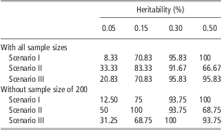
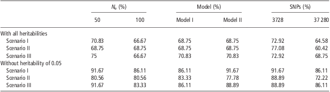
Percentage of the mean posterior heritability estimates obtained by the two Bayesian models that estimated the true heritability correctly (0.05, 0.15, 0.30 or 0.50)

For scenarios with sample size 200 excluded the total number of set-ups were 16.
The mean estimates are taken across all other set-up parameters. The total number of set-ups within each scenario was 24 for each of the heritabilities.
Population structure and size of heritability
The size of heritability was found to be the parameter of all the parameters evaluated in this study that had the highest effect on estimation precision. Table 2 shows the percentage of simulation set-ups, where heritability was not significantly deviating from the true heritability. The results showed that heritability was most difficult to estimate when the true heritability in the set-up was low, that is, 0.05. In each scenario, 24 set-ups with different parameters were simulated with a heritability of 0.05. The range of estimates that was within an acceptable range of the true heritability was between 8.33% and 33.33%. The worst scenario was the one where there was no relationship between individuals (scenario 1). The standard deviation for population set-ups with a heritability of 0.05 ranged from 0.01 to 0.08. Mean and median estimates were almost equal for each population set-up, but the heritability was mainly being overestimated. Increasing the size of heritability highly increased the number of estimates that were close to the true heritability. For the remaining three heritabilities (0.15, 0.30 and 0.50), the range of population set-ups that were tested to be in the range of the true heritability was between 66.67% and 95.83%.
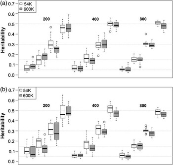
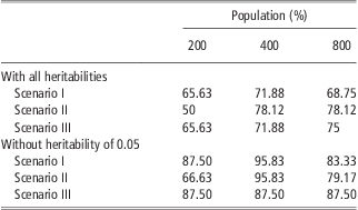
Increasing the sample size had a positive effect on estimation precision (Table 3). For sample sizes of 200 individuals, the estimation precision ranged from 50% to 65.63% for the amount of population set-ups, which were not found to be significantly deviating from the true heritability. For population set-ups with 400 individuals, precision increased to between 71.88% and 78.12%. Between set-ups with 400 and 800 individuals, only minor differences in precision were observed. When population size is low, the difference between estimates for same heritability varies more than when the population size is larger. In addition, the standard error of the heritability estimates decreased with increasing population size. An example of this can also be seen in Figure 1. In Table 3, we have also removed the heritability estimates for 0.05 from the comparison of the sample size. This increases the number of mean estimates that are within the range of the true heritability.
Heritability estimates from Model II. The single boxplots display the variation in heritability estimates among the 20 replicates from each population setup in scenario 2. For sample sizes of 200, 400 and 800 offspring, the model was tested for the potential to estimate heritability values of 0.05, 0.15, 0.30 and 0.5. The horizontal dotted lines indicate the true heritability for each population. (a) Estimates obtained from populations with an effective population size (N e) = 50 and (b) estimates obtained from populations with a N e = 100.

Percentage of the mean posterior heritability estimates obtained by the two Bayesian models that estimated the true heritability correctly
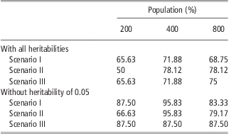
For scenarios without true heritability of 0.05, the total number of set-ups was 24.
The first-half of the table contains estimates including heritability of 0.05. In the last half of the table, the heritability of 0.05 has been removed from the estimates. The mean estimates are taken across all other set-up parameters than sample size. For each sample size, the total number of set-ups within each scenario was 32, when true heritability of 0.05 was included.
Increasing N e from 50 to 100 showed a minor tendency of decreasing precision. In scenario 2, there were no changes observed at all (Table 4). Excluding the estimates obtained for true heritability of 0.05 did highly increase the part of the estimates that were within the range of the true value.
Percentage of the mean posterior heritability that estimated the true heritability correctly

For scenarios without true heritability of 0.05, the total number of set-ups was 36.
The mean estimates are taken across all other set-up parameters than either of effective population size (N e), Bayesian models, marker density. For each of the parameters, the total number of set-ups within each scenario was 48, when true heritability of 0.05 was included.
Models and SNP marker arrays
Heritability was estimated with two Bayesian genomic prediction models (Model I and Model II). The overall results did not show any differences in precision between the two models (Table 4). Excluding the estimates obtained for the true heritability of 0.05 increased the part of the estimates that was within an acceptable range for both models with ∼10% to 22%. Both models were tested on the basis of the same output from each of the 48 different population set-ups that were obtained in each of the three scenarios. In ∼2/3 of all the set-ups, where heritability estimation deviated significantly from the true, both models did not estimate the true heritability correctly. For the rest of the set-ups, only one of the two models did not estimate the true heritability.
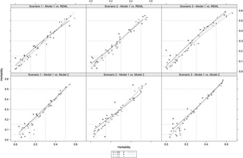
The two Bayesian approaches were also compared with an REML approach with estimation based on a genomic relationship matrix. Figure 2 shows that there were only minor differences in the estimates obtained by the three models. For the two Bayesian models, most estimates were very much alike, and therefore only one of the two models is plotted together with the REML model. As can be observed from the Figure 2, there was a variation between the REML and the Bayesian approach. However, the difference was only minor. For all parameters investigated in this study, we did not find any major differences in the size of estimates, when comparing estimates obtained with the three models.
Model comparison of the estimation precision with increasing population size (*, blue = 200 individuals; •, red = 400 individuals; ▪, green = 800 individuals). Heritability estimates obtained by the different models are plotted against each other. The corner of the dotted lines represents the true simulated heritability values, that is, 0.05, 0.15, 0.30 or 0.50. Lines represent the mean values of the heritability estimates obtained by the models for different population sizes. Comparison is only shown between Model I and REML and between Model I and Model II, because the two Bayesian models obtains estimates of equal size for most scenarios and population setups. REML = restricted maximum likelihood.

Minor differences were also observed for the two densities of SNPs (Table 4). Estimation precision was best when SNP density was low. Between 72.92% and 77.08% of the mean estimates were tested to be not significantly deviating from the true heritability. For the high SNP density, the range decreased to be between 60.42% and 68.75%. Excluding the estimates obtained for the true heritability of 0.05 increased the part of the mean estimates that were within the range of acceptable compared with the true heritability. The increase was approximately between 12% and 22%. Nevertheless, it was the lower SNP density that performed the best.
Comparing the density of SNP markers in combination with the performance by the two models revealed that Model I performed best when SNP density was low. In contrast, Model II performed best when SNP density was high (Supplementary Tables and Figures).
Mean deviation and variation
For true heritabilities of 0.05, heritability was in general overestimated. Mean heritabilities that were overestimated ranged from 87.50% (scenario 2) to 95.83% (scenarios 1 and 3) of the total number of mean estimates. Increasing true heritability to 0.15 reduced the amount of overestimation to between 54.17% (scenario 2) and 79.17% (scenario 1). A further increase of true heritabilities to 0.30 or 0.50 gave a surplus of underestimated mean heritabilities. For true heritability of 0.30, the range of overestimated mean heritabilities was between 29.16% (scenario 1) and 45.83% (scenario 2). And for true heritability of 0.50, the range of overestimates was further decreased to between 8.33% (scenario 1) and 25% (scenario 3; Figure 1 and Supplementary Tables and Figures).
Discussion
The aim of this study was to test the precision of two Bayesian genomic models to estimate different heritabilities based on phenotypic values and genomic data. Genomic data comprised a high- or low-density SNP distribution. The primary results of the study were as follows: (1) In 85.65% of the cases, the two Bayesian models were able to estimate heritability in populations composed of a limited number of close relatives and when true heritability was 0.15 or higher; (2) the size of the true heritability was the only parameter that exhibited a major impact on estimation precision. The overall results show that low true heritabilities were most difficult to estimate, and that both models tended to overestimate the low true heritabilities; (3) the two genomic models used in this study performed equally well; and (4) for the sample sizes used in this study, no benefits were gained from including an SNP array with increased density of SNP markers. Increasing the density of SNPs instead decreased the estimation precision.
Population structure
In this study, heritability was estimated based on populations originating from different selection scenarios. For true heritabilities of 0.15 or higher, no major differences in estimation precision between the different selection strategies were in general found. For small samples, however, that is, 200 individuals, biases were found, but when data sizes increased the bias reduces. For heritabilities of 0.05, scenario 1 was found to have more estimates that deviated significantly from the true value than was found for scenarios 2 and 3 (Table 2). For scenario 1, true heritability of 0.05 was only possible to estimate in populations of 800 individuals, with low-density SNP markers and with Model I. For scenarios 2 and 3, the differences were less pronounced for true heritability of 0.05. In scenario 1, individuals were randomly selected from the base population and without having any close relationship between the individuals. In the other two scenarios, a relationship structure consisting of four half-sibs was added. This would be expected to provide scenarios 2 and 3 with a higher LD compared with scenario 1. However, the observed LD showed that there were only minor differences between the three scenarios. We can therefore not draw the conclusion that the differences between scenarios can solely be due to differences in LD. Increasing the heritability did also diminish the difference between the scenarios. This indicates that the estimation precision of the two Bayesian models was less affected by the population structures investigated in this study. Comparing the standard deviations obtained for each parameter did not reveal any difference between the three scenarios. For each scenario, an increase in heritability tended to increase the standard deviation (Supplementary Tables and Figures).
In relation to sample size, the results showed that a sample size of 400 individuals is enough to obtain precise estimates. Increasing the sample size to 800 gave different outcomes. In Table 3, a summary of estimates is given with and without estimates of true heritability of 0.05. By removing the estimates of low true heritability of 0.05, the tendency is that the other parameters only express a minor impact on the precision of the estimates. Including heritabilities of 0.05, an increasing sample size also increased precision in both scenarios 2 and 3. Excluding heritabilities of 0.05 only had a minor influence on precision when increasing sample size. This illustrates that increasing sample size has a greater influence on the precision, when heritability is low compared with when heritability is higher. Despite that the estimation precision of the mean only increased a bit with increasing sample size. It is still important to notice that the variance between replicates decreases. This means that the estimates from each replicate resemble each other more with increasing sample size (Figure 1).
Increasing N e was found to decrease precision. Despite the fact that the differences detected in this study were only minor, it still indicates that attention should be paid on sample size if N e is very different from the values that we used in this study.
Genomic model performance and SNP density
The main challenge we encountered was inadequate low heritability estimates (0.05), due to overestimation. This might be explained in the manner variance is estimated. As estimated variance can only have positive values, there will be an automatic boost of the mean towards overestimation as heritability approaches zero. The MCMC chain of genetic variance estimates also revealed a tail of overestimates (results not shown), contributing to the total overestimates. A possible solution to this problem could be to use the mode of the genomic values instead of the mean, as the mode is less prone to upwards bias.
The two models applied in this study performed in general equally well in estimating variance components and heritability. However, a closer examination revealed that Model II was better at estimating true heritabilities of 0.15. Across the three scenarios, 13.89% of the estimates obtained by Model II were significantly deviating from the true heritability of 0.15. For Model I, this number was increased to 33.33% across the three scenarios. This indicates that Model II is not affected from the prior settings, which were based on a population with a true heritability of 0.30. If the prior setting would have affected the estimates, we would have expected that Model II should be more precise in estimating the true heritability of 0.30 compared with Model I. Or, in case both models performed equally well with true heritabilities of 0.30, we would have expected that Model I would have been better at estimating the lower heritabilities, as Model II would be biased towards the heritability of 0.30.
The results indicate that when heritability is low, it is better to use a mixture model (Bayes C). In addition to reducing the number of SNPs with greater effect on the trait, the model also reduces the influence from the major part of SNPs with no effect on the trait. Therefore, Model II should be the method of choice for low heritabilities of 0.15. For the moderate true heritabilities (0.30 and 0.50), Model I was found to be most precise. For heritabilities of 0.30, the two models failed 2.78% (Model I) and 5.56% of the cases (Model II) of the set-ups and for heritabilities of 0.5 the models failed in 8.33% (Model I) and 19.44% (Model II). This indicates that for these levels of heritabilities one should consider to use models similar to Model I, which apply the same weight to all SNPs. Comparing the estimates from the two Bayesian models with the estimates from the REML approach revealed that there were no larger differences in the capabilities of the different model approaches in estimating heritabilities (Figure 2).
Comparing density of SNPs with models revealed a minor difference between the two models. Model I was the model that was most sensitive to SNP density, and performed best when SNP density was low. In contrast, Model II was less sensitive and there were no real differences observed in precision between the two densities of SNPs. This can be explained by the prior settings in Model II. With the prior settings, only a few of the SNP markers are modelled with a high effect. In the initial set-up, the difference in SNP density was 10-fold. With the prior settings, this difference was reduced. Here the number of SNPs was now 932 v. 1305 for high and low density of SNPs. This could balance the difference between the distributions and thereby also balance the precision when using one of the two SNP distributions. In contrast to Model I, we only interpreted the expected average fitted variance (Janss, Reference Janss2010). This meant that each SNP marker from the high-density set-ups only contributes with one-tenth of the effect compared with the contribution from one SNP taken from the lower density SNP marker set-up.
The general expectation from higher SNP density around QTLs is greater accuracy in heritability estimates due to an increase in LD between SNP and QTL (Sved, Reference Sved1971; Goddard et al., Reference Goddard, Hayes and Meuwissen2010). However, the results indicated the two genomic models did not access or correctly interpreted the information provided by the high-density SNP arrays. Especially for set-ups with a low sample size and a low heritability, our results show that Model I tend to highly overestimate the variance components, resulting in both a high mean and median (Supplementary Materials). It is possible that increasing sample size would improve estimation precision for the set-ups with high density of SNPs.
In conclusion, the two Bayesian models estimated heritability equally well in each of the three selection scenarios. Further, the sizes of the estimated heritability were close to the true value of heritability, and the estimates resembled each other well across selection scenarios. This indicates that SNPs capture the variance/co-variance structure generated in the past, and can therefore be used to estimate heritability. However, results also demonstrated that true heritability estimation failed mainly in setups simulated with a low true heritability (0.05). This could be altered by a larger sample size, as increasing sample size was shown also to have a moderate effect on precision. Density of SNPs and effective population size did not show a major impact on the precision of estimated heritability. Comparing the two Bayesian models with a REML approach did not reveal any major differences in precision. We therefore conclude that the two Bayesian models used in this study can be applied for estimation of moderate heritabilities in a genotyped population with unknown population structure.
Acknowledgements
This study is part of the Danish-Swedish Milk Genomics Initiative (www.milkgenomics.dk) supported by the Danish Agency for Science, Technology and Innovation, Danish Cattle Federation and Arla. The authors would like to thank Anders Christian Sørensen for helpful comments on the writing.
Supplementary materials
For supplementary material referred to in this article, please visit http://dx.doi.org/doi:10.1017/S1751731112002017