Introduction

Investigations of the global climate system with coupled atmosphere-ocean general circulation models (GCMs) most often ignore the effects of sea-ice dynamics. Only recently have some models included simple treatments of ice dynamics; they have shown its importance in the simulation of sea ice, global climate and sensitivity to climate change (Reference Washington and MeehlWashington and Meehl, 1996; Reference Pollard and ThompsonPollard and Thompson, 1994). Such models still contain parameterizations of important physical processes, such as energy fluxes through sub-gridscale leads, which should progress as modeling resolution and methods are improved.

The Climate System Model (CSM) is a coupled atmosphere-ocean GCM recently developed at the National Center for Atmospheric Research NCAR) for use by the modeling community. It includes a dynamic-thermo-dynamic sea-ice model that resolves many of the physical processes that control interactions between sea ice and climate. In this paper, we present the results of the simulation of sea ice in both hemispheres from the first coupled experiment of the CSM.

Model Description

The CSM comprises the NCAR Community Climate Model version 3 (CCM3) atmospheric GCM at 2.8° × 2.8° resolution and 18 vertical levels (Reference KichlKiehl and others, 1996); a global ocean model of approximately 2° × 2° resolution and 45 vertical levels (NCAR Ocean Section, 1996); and a dynamic-thermodynamic sea-ice model (Reference Bettge, Weatherly, Washington, Pollard, Briegleb and StrandBettge and others, 1996). These model components are linked by the NCAR Flux Coupler (Reference Bryan, Kauffman, Large and GentBryan and others, 1996), which computes the fluxes of mass and energy at the interfaces between the model components. A brief description of the sea-ice model will be given here; more complete descriptions of all components can be found in the references given.

The sea-ice model component is based on that used by Reference Washington and MeehlWashington and Meehl (1996) in a global atmosphere-ocean GCM. the model uses the Arakawa B-grid in spherical coordinates, with a fixed longitudinal resolution of 2.4° and varying latitudinal resolution from 2.2° at 20° (N and S) to 1.2° poleward of 60°, and includes a sea-ice gridcell al 90° N. The time-step of the ice model is currently set at 1200 seconds and resolves the diurnal cycle. The thermodynamic formulation is based on the three-level Reference SemtnerSemtner (1976) model, with minor modifications for its interface with the Flux Coupler. The Flux Coupler computes fluxes of heat, mass, radiation and momentum separately over the ice-covered and ice-free (ocean) fractions of each gridcell. so that open leads can absorb energy or refreeze. The growth of new ice in the open ocean and leads is passed from the ocean model, and contributes to lateral growth up to a maximum concentration. Surface albedo is dependent on snow depth, and is reduced for melting ice and snow. The net flux of fresh water is Computed from the growth and inch of sea ice, using a constant salinity of sea ice of 4 ppt, and from fresh snowmelt. Presently, there is no river runoff included in the CSM.

The sea-ice model dynamics are taken from the formulation of Reference Pollard and ThompsonPollard and Thompson (1994) for the cavitating fluid ice rheology of Reference Flato and HiblerFlato and Hibler (1992). For gridcells under convergent stresses, ice pressure is incremented to reduce convergence. For convergent points, where the ice pressure is less than the maximum ice strength (see Reference Flato and HiblerFlato and Hibler, 1992), the divergence of ice velocity should be negligible. However, for these points, it was seen that the divergence can remain as much as −1 × 10⁻⁷ s⁻¹, even after 1000 iterations of the solution. This residual convergence can, under persistently convergent stresses, allow ice thickness to increase at a rate of greater than 300% a⁻¹ at points where the ice should be incompressible.

To correct for the excess ridging of ice, the advection scheme was formulated into separate divergence and advective terms. For gridcells with residual convergence, the divergence term is set to zero, eliminating any excess ridging. The volume of excess ridging is then redistributed to the remaining divergent ice pack.

Results

The CSM experiment described here was conducted by the CSM Principal Investigators Group at NCAR. The sea ice and ocean were initially coupled and run together for 230 years, with mean monthly atmospheric forcing from a simulation with CCM3. During this spin-up, the residual convergence in the ice model was identified and the corrections described above were implemented. The CCM3 atmosphere was initially run separately using observed SSTs, before coupling to the ocean and ice models. The fully coupled system was run for 25 years, the results of which are presented here.

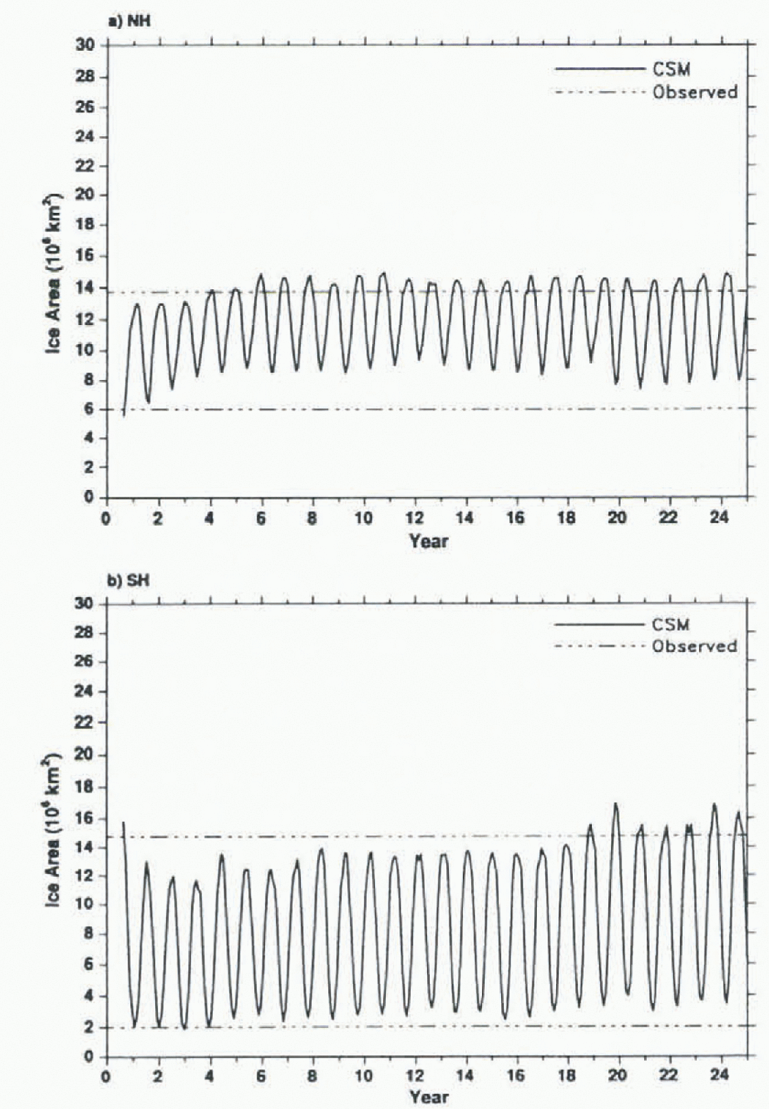
The total sea-ice-covered areas in the Northern and Southern Hemispheres are shown in Figure 1. The Arctic ice-area maxima are slightly greater than the mean maximum analyzed by Reference Gloersen, Campbell, Cavalieri, Comiso, Parkinson and ZwallyGloersen and others (1992) from remotely sensed ice concentrations, while the Antic minima are considerably greater than observed. The Antarctic ice area grows slowly over 25 years, in response to a slight cooling trend in the modeled SST, to approximately 10% greater than the observed mean maximum and minimum values. A more recent CSM experiment has reduced the trends in ice area and SST considerably.

Fig. 1.

Total ice-covered area in the 25 year CSM run for a) the Nothern Hemisphere (NH) and b) the Southern Hemisphere (SH), and observed maximum and minimum areas (dashed lines).

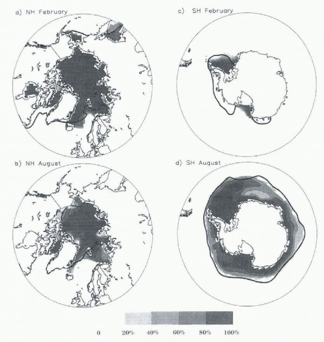
The Arctic ice concentrations (Fig. 2a, b) are primarily 96−99% in February, and extend farther south in the Greenland, Iceland and Norwegian Seas (GIN) than the observed ice edge. Similarly, in August, the ice pack is too extensive in Bain Hay. the CiIN seas, and the Arctic basin. While there was a strong North Atlantic thermohaline circulation in this simulation, the SSTs in the GIN seas remained much too cold, implying there was insufficient ocean-heat transport to melt ice. The Antarctic sea-ice concentrations (Fig. 2c, d) and the position of the February ice-edge in particular, are closer to observations (the Antarctic Circumpolar Current simulated by the ocean model tends to constrain the ice edge closer to observations). However, the simulation indicates that the Ross Sea remains ice-covered year-round, in contrast with observations, and it has too little ice cover in the Bellingshausen Sea.

Fig. 2.

Mean monthly ice concentrations for a) Northern Hemisphere February, b) Northern Hemisphere August, c) Southern Hemisphere February, and d) Southern Hemisphere August. Solid lines are observed mean ice edges adapted from Reference Gloersen, Campbell, Cavalieri, Comiso, Parkinson and ZwallyGloersen and others (1992).

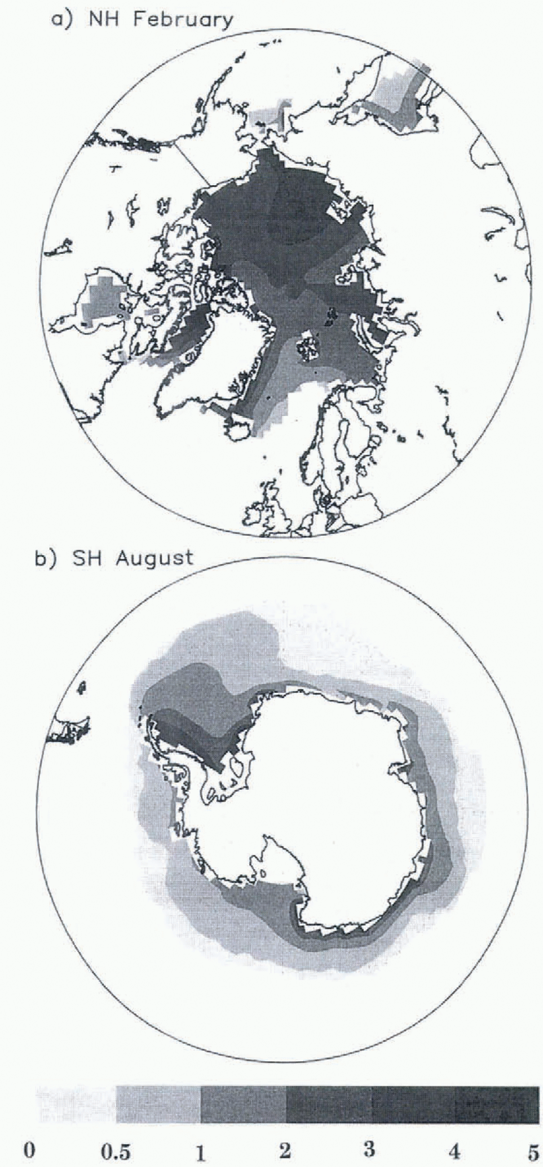
The Arctic ice thickness in February (Fig. 3a) builds up to approximately 5m in the Chukchi and East Siberian Seas, but is only 3 m north of Greenland, lacking the observed pressure ridging against North America. This thickness pattern is created by the direction of ice drift in response to wind and current stresses. In Baffin Bay, simulated ice thicknesses of 5m exist year-round as an undesirable result of the redistribution process, which has been improved in recent experiments by limiting the redistribution to within the Arctic basin.

Fig. 3.

Mean monthly ice thickness (m) for a) Northern Hemisphere February, and b) Southern Hemisphere August.

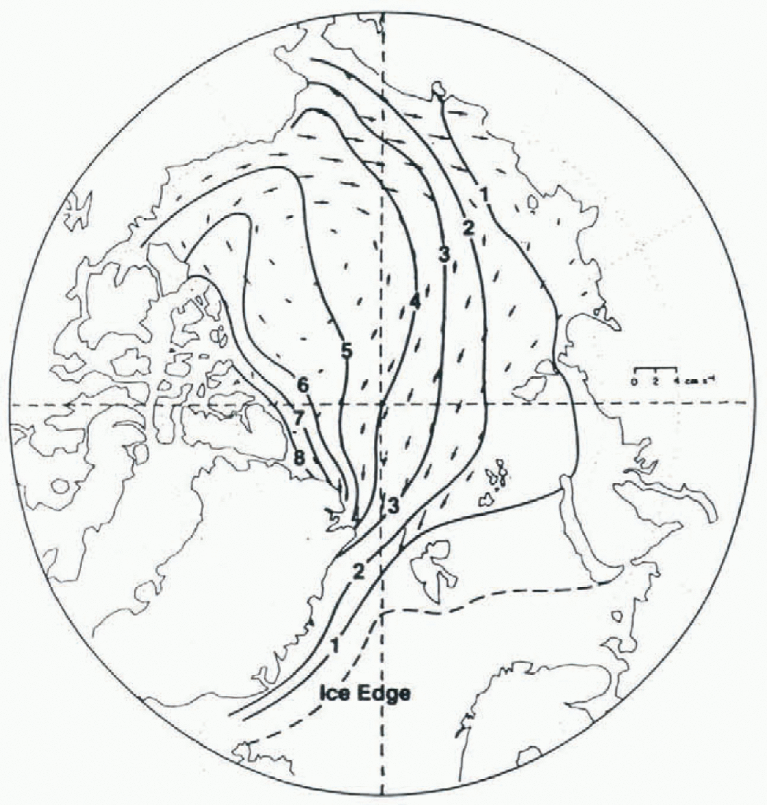
The simulated ice-velocity field (Fig. 4) shows an anti-cyclonic Beaufort Gyre, but lacks the observed Transpolar Drift Stream. The modeled ice velocities near the Pole are directed towards Alaska and not towards Fram Strait as observed. Figure 5 shows the observed mean ice drift from buoy data (Reference Colony and ThorndikeColony and Thorndike, 1984) and the observed winter ice thickness from submarine data (Reference Bourke and GarrettBourke and Garrett, 1987).

Fig. 4.

Annual mean ice velocity in Northern Hemisphere from CSM

Fig. 5.

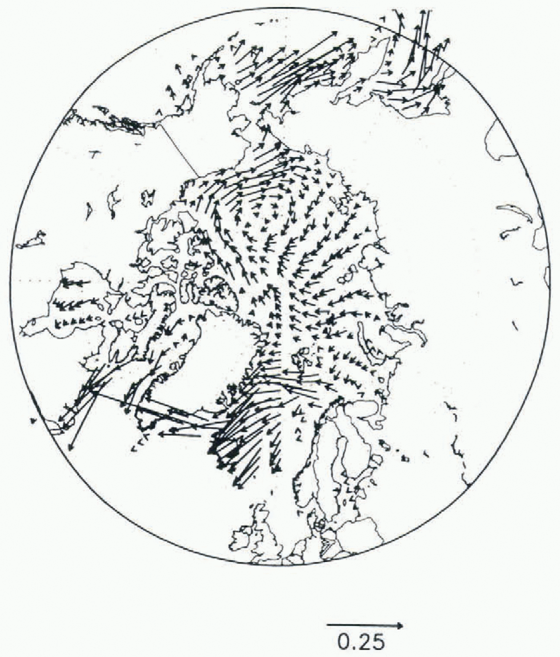
Observed mean ice drift (arrows) from Reference Colony and ThorndikeColony and Thorndike (1984) and winter-ice thickness (m) from Reference Bourke and GarrettBourke and Garrett (1987).

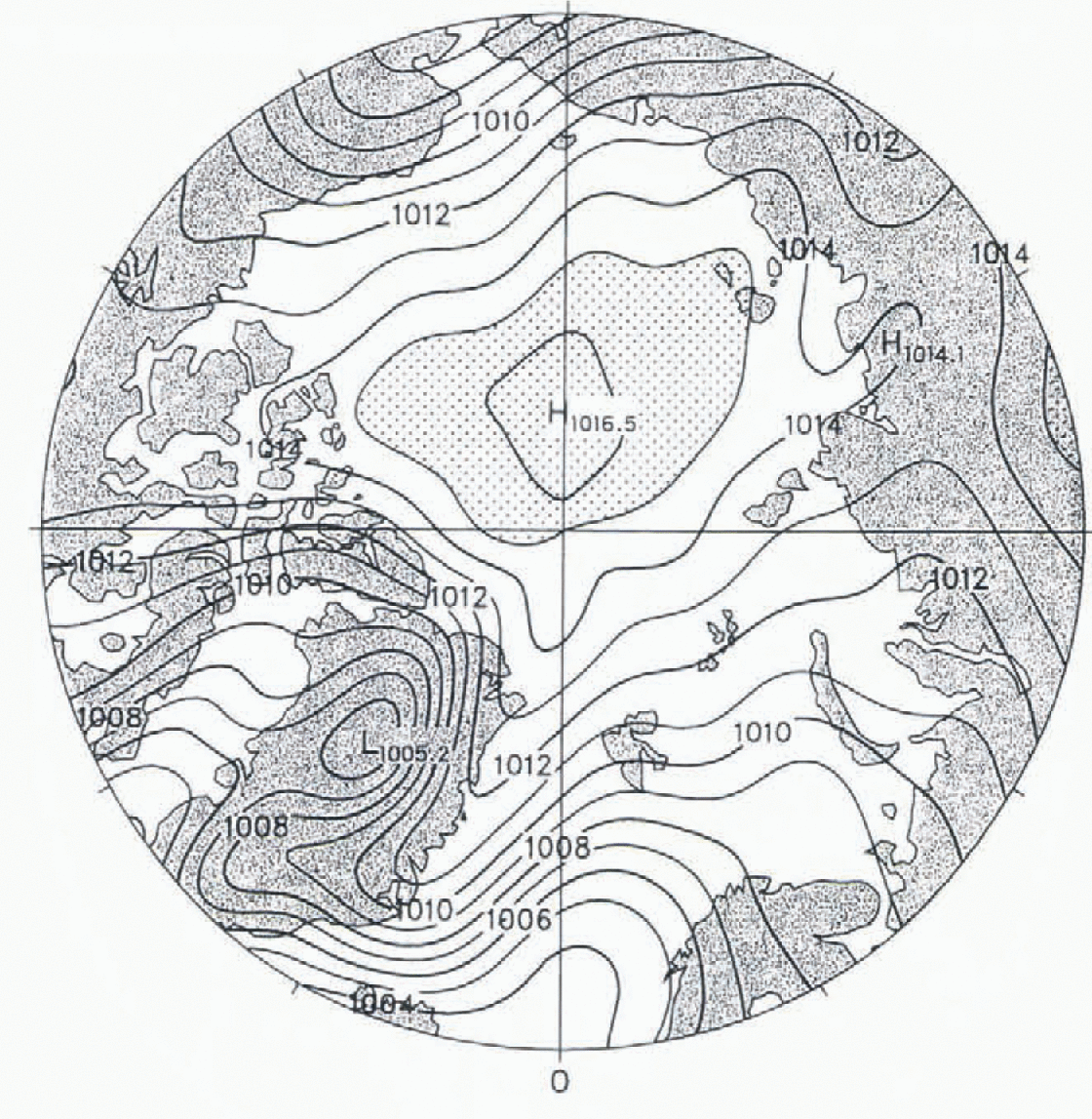
While the ice-velocity field differs from observations, it appears to be the appropriate response to the atmospheric model winds. The sea-level pressure from the CSM (Fig. 6) shows an anticyclonic Beaufort High displaced towards Siberia, which contributes to the ice advection towards Alaska and the Chukchi Sea. This demonstrates the rather high sensitivity of the Arctic ice velocity and ice-thickness distribution to simulated atmospheric forcing: while the atmospheric pressure patterns are not too far from observations, the ice motions are considerably different.

Fig. 6.

Annual mean atmospheric sea-level pressure (h Pa) from CSM. Contour interval is 1 hPa, with the pressure in the stippled region greater than 1015 h Pa.

The Antarctic ice thickness in August (Fig. 3b) is primarily 0.5−1.0 m, with pressure ridging up to 3.5 m against the Peninsula. This is comparable to the analysis by Reference Harder, Lemke, Johannessen, Muench and OverlandHarder and Lemke (1994) of sea-ice thickness measurements from the Winter Weddell Gyre Study (WWGS), which show an average thickness in the eastern Weddell Sea of 0.5−1.0m, increasing towards the western Weddell to a range of 1.0−3.0 m.

Conclusions

The results of the CSM sea-ice model in a climate simulation show that sea ice responds appropriately to the modeled climate, but the coupled system produces some unrealistic wind forcing and ice motion. The simulation of sea ice is more realistic in the Antarctic than in the Arctic, in part because Antarctic sea ice is more divergent and easier to model. The pattern of wind stress from the atmospheric model produces persistent convergence of ice in the Chuckchi Sea. In addition, the numerical solution of the cavitating fluid ice dynamics was found to allow excessive pressure ridging under this convergent pattern. This aspect of the cavitating-fluid model has not been documented previously, presumably since earlier models used observed wind forcing that serves to drive greater ice export through Fram Strait. Improvements to the cavitating-fluid solution to eliminate the excess convergence of ice are being investigated.

Coupled atmosphere-ocean-ice model simulations in general are affected by model initialization, spin-up and model limitations that lead to climate drift. The sea-ice model, with the limitations discussed herein, reproduces some aspects of the observed polar sea ice, and provides the feedbacks between ice, atmosphere and ocean that are important for studying the global climate.