A. Tuning forks

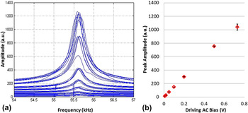
As a control, Fig. 1(a) presents common frequency responses of a macroscopic TF, measured by analyzing the AC bias on a voltage divider across the TF with a lock-in-amplifier (arbitrary units are shown) during frequency sweeps across 3 kHz in 25 Hz steps (i.e., 120 points per line) in air. For each frequency sweep past the primary resonance at approximately 55.6 kHz, 7 distinct driving amplitudes are used from 10 to 730 mV (peak to peak). The results for each condition are offset by 40 a.u. for visual clarity in the figure, with the strongest driving voltage offset by 240 a.u. and the weakest barely rising above 0. The mean peak amplitude is displayed for each of these conditions in Fig. 1(b), with error bars representing the standard deviation based on 5 measurements for each driving amplitude to establish repeatability. As expected, these results indicate a nearly perfectly linear correlation between the driving amplitude and the maximum response of the TF (R ² = 0.9985).

FIG. 1.

TF response (arbitrary units) as measured by a voltage divider while sweeping the driving frequency past the 55.56 kHz primary resonant frequency multiple times for 7 distinct AC amplitudes (a), revealing a linear maximum response with driving amplitude (b) and ±standard deviation error bars of 1–5%. Note that each set of frequency sweeps at distinct driving amplitudes is offset by 40 a.u. in (a) for clarity.

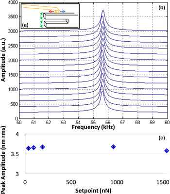
Mounting the same TF as studied in Fig. 1 in an AFM and contacting one of the tines as sketched in Fig. 2(a), the amplitude is directly measured by monitoring deflection of the high frequency AFM probe and again analyzing the signal with the lock-in-amplifier. For a fixed driving amplitude of the TF, 15 consecutive frequency sweeps were made, Fig. 2(b), again each offset for visual clarity (by 200 a.u.). The sweeps are visually indistinguishable except for subtle shifts in the peak frequency, which amount to a maximum of ±5 frequency steps of 10 Hz, attributed to thermal effects for these measurements made in ambient conditions. Importantly, these 15 measurements are actually 5 groups of 3, each acquired with a distinct AFM contact force (i.e., setpoint) ranging from 39 to 1540 nN. Figure 2(c) displays the average maximum amplitude for the peaks as a function of this setpoint, along with the essentially negligible standard deviation. These results indicate a nearly constant electromechanical response of the TF except for the highest AFM load (1.5 µN). The units here have been converted to actual root mean square (rms) nanometer amplitudes via a conversion factor of 48.1 nm/V as described in the methods section. The results yield an effectively flat response for the resonant frequency as well, not shown for brevity.

FIG. 2.

Sketch of in situ AFM and TF structure (a), AFM-detected amplitude (shown in raw arbitrary units) during 15 frequency sweeps (b) driving the resonance of the same TF as in Fig. 1, and the resulting peak amplitude (calibrated to nanometer of rms amplitude, with standard deviation error bars) as a function of the setpoint force (c).

Of course at some high load the AFM tip may cause the TF to behave like a damped harmonic oscillator. While this threshold could be near 1 µN, a barely apparent maximum in Fig. 2(c), we have not explored this possibility since higher loads are not reliable with the AFM probes and system used in these experiments. In fact, the 1 µN condition required 5 V of setpoint deflection for this lever and alignment with the AFM, while the slightly diminished response at a 1.5 µN load necessitated an 8 V setpoint, where nonlinearities of the photodetector may somewhat mask the true behavior. Therefore, loads much less than 1 µN are otherwise used throughout the remainder of this work (typically ∼200 nN), where the contacting AFM can reasonably be assumed not to perturb the simple harmonic oscillator behavior of the TF. In fact, the experiments could be performed faster by sampling fewer frequencies and fitting the results to a simple harmonic oscillator response, but instead the pure data, maximum signals, and frequencies for these maxima are considered throughout.

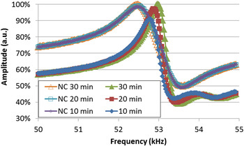
Returning the measurement configuration to a voltage divider circuit instead of AFM detection of the tine amplitude, the TF response was next measured in liquid, Fig. 3. Specifically, the tines were submerged into a mixture of cell culture media and buffer solution, with and without the addition of a nanofibrous collagen that typically gels in approximately 30 min. The peaks between 52.8 and 53 kHz, acquired every 10 min as noted, display a subset of more than 20 regularly repeated frequency sweeps during curing of the nanofibrous collagen gel. The amplitude, and the frequency, clearly rise smoothly with curing time. For comparison, an identical control experiment was also performed with the cell culture media and buffer solution alone, i.e., without the collagen and hence a gel will not form. The peaks for this no-collagen case at ∼52.5 kHz (labeled as ‘NC’ in the plot) are stable over the same duration, supporting use of such TFs to monitor curing of gels.

FIG. 3.

TF frequency response to monitor curing of a nanofibrous gel as a function of time, as compared to a control experiment without the gelling agent (labeled NC).

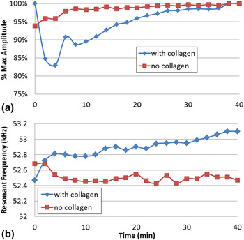
TF spectra similar to those in Fig. 3 were in fact acquired every 2 min. Analyzing the maximum amplitudes and frequencies leads to Fig. 4. Beyond 10 min, an increase in the TF resonant amplitude (a) and similarly the resonance frequency (b) is observed, implying an increase in viscosity as expected during gelling. In the first 10 min, on the other hand, the response shows certain frequency drift, possibly suggesting the detection of distinct reaction stages, but most likely related to the temperature evolution during the early stages of the measurement. While endothermic or exothermic reactions can be detected via the temperature sensitivity of the TFs,^{Reference Xu, You and Zhao62} it is more likely that the first 4 data points are indicating nonlinearities during thermal equilibration of the system overall because even though the measurements are performed in a thermally isolated chamber, the lid is open at time zero to add the rat tail collagen HC and initiate the reaction. This possibility is supported by the identically acquired TF response for the control conditions, i.e., without the collagen gel, which is also plotted for an equivalent overall duration. The resonant frequency remains essentially constant as anticipated, with a less substantial but still apparent drift in the first few measurement points (∼5 min), therefore attributed to thermal equilibration effects.

FIG. 4.

Resonant amplitude (a) and frequency (b) for a TF as a function of time when submerged in a liquid of cell culture media, PBS, NaOH, and collagen during curing (‘with collagen’) as compared to a stable control measurement without the curing collagen gel (‘no collagen’).

The gel is expected to have fibers and pores on the ∼10 nm scale, such that it is important to know the amplitude of the tines to relate the magnitude of the mechanical perturbations they cause to the surrounding effective microstructure. Accordingly, the same TF was mounted in an AFM in air for direct measurements of the resonant amplitude normal to the TF axis, i.e., the direction of maximum amplitude. Rotating the horizontally mounted TF by 90° would allow shear of the TF tines to be detected instead, or even leveraged as a fast scanner as in some high speed AFM systems.^{Reference Humphris, Miles and Hobbs63}

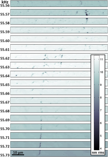
Figure 5 presents a montage of 18 corresponding AFM images of the TF, each 5 × 80 μm (1:16 aspect ratio), all acquired in the same location where the left edge is aligned with the free end of the imaged tine (4 mm from its base and therefore where the normal amplitude should be a maximum). The displayed contrast does not present height as is common with AFM, since it is essentially identical for these multiple images of a single area. Instead, the distinct images map the AFM-detected local amplitude of the tine, for a range of specific driving frequencies as noted. Specifically, the images sequentially step through the primary resonant peak of the TF, from 55.56 to 55.73 kHz in steps of 10 Hz. The nano- to micrometer sized features are discussed later in the manuscript, but initially the brighter overall image contrast (stronger amplitude) near 55.63 kHz stands out, revealing the vibrational resonant peak. While the amplitude should also be strongest at the free end of the tines and hence the left edge of each of the images, this is difficult to discern from the general trends of these amplitude contrast images alone.

FIG. 5.

18 images of the TF amplitude as a function of frequency for a 5 × 80 μm area near the end of a 4 mm tine (just beyond the left edge).

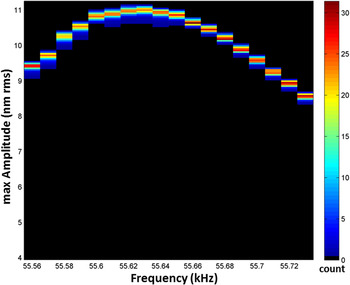
To better visualize the overall amplitude and frequency response of the TF tine, a two-dimensional histogram of the entire dataset in Fig. 5 is shown in Fig. 6. In this representation, the histogram count is displayed as color contrast. The histogram bins are established for the 18 discrete driving frequencies (i.e., images) with steps of 10 Hz as indicated in the x-axis of the figure, and for a range of possible vibration amplitudes as identified by the y-axis based on steps of 2 pm rms. At each frequency, the detected amplitudes are tightly grouped, indicating a relatively uniform response in the imaged region. Optical interferometry measurements of the same structure, with its common micrometer scale or worse lateral resolution, could resolve similar average signals. However, interferometry cannot differentiate the nanoscale responses evident in Fig. 5.

FIG. 6.

Two-dimensional histogram of the number of image pixels (i.e., relative area of the imaged region of the TF, color contrast) for defined amplitudes (y-axis) and frequencies which in this case means the 18 discrete images (x-axis).

Using such high spatial resolution, multiparametric data, maps of a range of properties such as the local maximum amplitude ideally can be determined down to the resolved pixel size in the initial AFM images. This is achieved by (i) simply “drilling” through the stack of distinct images (i.e., Fig. 5) for any given image pixel as described elsewhere;^{Reference Bosse, Grishin, Kolosov and Huey64} (ii) calculating and recording the image frame at which the contrast is strongest (e.g., the frequency corresponding to the peak amplitude), or it reaches some other indicative magnitude (e.g., where a phase signal reaches 90°, current reaches 0 nA, etc.); and (iii) repeating this process for every pixel in the imaged region. In this case, the resulting images of the maximum amplitude, frequency for the maximum amplitude, etc. can then be easily compiled. The spatial resolution of such maps depends on two parameters, any uncorrectable spatial drift during the experiment (linear or measured drift can easily be accommodated), and of course the initial information density (pixel size). The pixel densities for the images of Fig. 5 are relatively modest (∼312 nm on a side), but practically can extend down to the limit of the AFM tip contact area (∼5 nm for similar condition contact-mode AFM images and tips). This general concept has previously been used for efficient, high resolution mapping of conductivity,^{Reference Bosse, Grishin, Kolosov and Huey64} photoconduction,^{Reference Kutes65} stiffness,^{Reference Huey66} and friction coefficients.^{Reference Bosse, Lee, Huey, Andersen and Sutherland67}

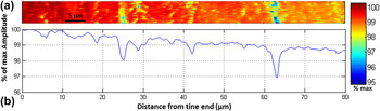
Of course both the resonant frequency and amplitude for the millimeter scale TF are expected to be relatively uniform when imaged on the micrometer scale with AFM. Indeed, calculated images of the maximum amplitude and frequency for this maxima (i.e., resonance) simply correspond to the contrast in the single image of Fig. 5 with the strongest signal (i.e., at 55.62 kHz). Therefore, for this millimeter-sized feature, an image of the average vibrational response of the tine as a function of the distance from its end is both more revealing, and more appropriate given the spatial scales of the device. Specifically, (i) the 18 images of a single area from Fig. 5 are each normalized to the maximum amplitude at that frequency (which in fact occurs at the left edge of each image, i.e., nearest to the end of the tine); (ii) drilling through this data pixel by pixel as described before, the average normalized amplitude with respect to the end of the tine is calculated; (iii) this is repeated for every image pixel to generate the average amplitude response for the last 80 µm of the tine, Fig. 7(a). A cross section of this entire result, Fig. 7(b), now reveals the general decrease in amplitude from the tine end toward the base that was expected but visually unapparent in the raw data of Fig. 5. In particular, the measured change in amplitude over the 80 μm imaged length is ∼1.5%, which compares favorably with the fraction of the overall 4 mm tine length that is directly investigated, i.e., the last 2% of the tine.

FIG. 7.

Map of average normalized amplitude (a) and cross section of the result (b) from Fig. 5 revealing a 1.5% decrease in the normalized vibrational amplitude over the last 2% of the tine length.

It is important to note that localized enhancements of the electromechanical response, as well as topography induced artifacts which tend to degrade the measured response, can superimpose on such results. In this case, poorly bound particles on the surface yield apparently vertical stripes of diminished amplitude in Figs. 5 and 7, due to poor mechanical coupling between the tip, particle, and/or tine. Here, inconveniently this is coincidentally convoluted with several micrometers of thermal drift in the y-direction. This can be accommodated in future measurements with feature tracking, or using high speed AFM to minimize thermal drift. Regardless, these model results validate the use of AFM for in situ measurements of electromechanical systems. The maximum measured amplitude of approximately 11 nm (rms) for the tines further confirms the applicability of such TFs for investigating curing effects of nanofibrous gels, since the vibration magnitude is on the same order as the gel porosity. Future investigations will focus on the TF response to gel curing time for a much larger range of vibrational amplitudes, which should provide further insight into the mechanical properties of the mesoscopic interconnected network of fibers.

B. MEMS

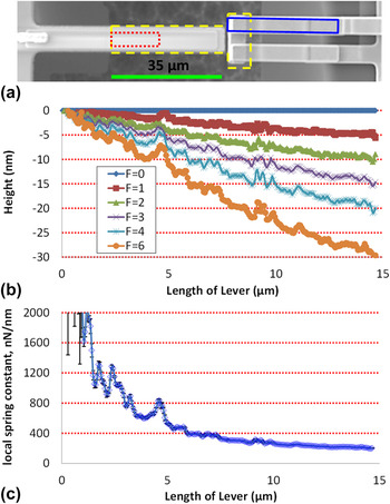
Similar in situ investigations on much more AFM-scale structures such as MEMS have also been achieved. Figure 8(a), for example, depicts a secondary electron secondary electron scanning electron microscopy (SEM) image of a T-shaped cantilever, where the suspended T-structure is outlined by light dashed lines. The AFM is first scanned along this 35 μm long microcantilever within the indicated dark dotted region, such that the left edge identifies the end of the underlying supporting structure (the ‘suspended base’). Two primary measurements are conducted in this manner, one to determine the spring constant of the MEMS structure, and the other to monitor its electromechanical actuation in situ. Overhanging the T-shaped structure are two gold cantilevers approaching from the right of Fig. 8(a). These independent electrical leads are suspended above the T-section, allowing them to be connected when the T-shaped cantilever contacts them both (upon actuation by sufficiently biasing the PZT thin film). Additional AFM measurements on one of these overhangs, within the slightly rotated rectangle, are also described below.

FIG. 8.

Secondary electron SEM image of a MEMS structure suspended where noted by the dashed lines (a), AFM measured height profiles of the MEMS structure for a sequence of distinct AFM applied loads up to 6 µN, all imaged from the base of the suspended region within the area sketched by the dotted lines (b), and the corresponding local spring constant calculated based on Hooke's law every 63 nm (each original image pixel in the x-direction) along the lever length (c).

For a given AFM setpoint force (F), the active MEMS lever should respond similar to an AFM cantilever, and thus deflect normally (in the z direction) proportional to the load according to Hooke's law (z = F/k _c). But since the load is applied by the AFM tip at every imaged location (l) while scanning along the lever, it is important to note that the measured change in height due to distortion of the MEMS structure at that location (z _l) can reveal a local spring constant (k _{c, local}) according to Eq. (1). Only at the end of the lever (l = L) would the conventional spring constant (k _c) be reached.

(1)$${{\bi{k}}_{{\rm{c}},\,{\rm{local}}}} = {{\bi{k}}_{\rm{c}}}{\left( {{L \over l}} \right)^3} = \left( {{{Ew{t^3}} \over {4{L^3}}}} \right){\left( {{L \over l}} \right)^3} = \left( {{{Ew{t^3}} \over {4{l^3}}}} \right) = {F \over {{z_{\rm{l}}}}}\quad .$$

Accordingly, Fig. 8(b) presents the measured height along the MEMS lever from a multiparametric sequence of consecutive images similar to Fig. 5, except that height is acquired with a different setpoint for each image frame. For brevity only the average height across the lever (in the y-direction) is displayed for position (l) at each load (F), but of course it could be fully mapped. To accommodate tilting in AFM images that is omnipresent, though constant for a given imaging session, each height profile is adjusted so that the linearly extrapolated MEMS distortion for zero applied force is exactly zero (i.e., a constant background slope is subtracted from all data, as is common in SPM analysis). Visually, the deflected height of the MEMS lever does indeed appear to be linearly proportional to the applied force for any given position (l) along the length of the lever.

Calculating the slope at every single location, resolved down to a spacing of 63 nm, yields the measured local spring constants, Fig. 8(c). The fitting quality R ² coefficient (not shown) indicates a good fit except near to the base of the structure (>0.98 beyond 1 µm), in which deflection is minimal and hence the instrumental signal-to-noise ratio is expected to introduce error. In fact error bars are overlaid displaying the standard deviation of the slope for each position, but are only prevalent nearest the lever base. This validates the linear (Hooke's law) fit, as well as the linear approximation to determine the suitable baseline height and slope when calculating the F = 0 condition.

For a fixed lever width, thickness, and material parameters, according to Eq. (1) the local spring constant is expected to change with position, inversely proportional to the 3rd power. These measured results do not, however. This is likely due to the fact that the MEMS structures are more complex compared to a simple cantilever beam, with multilayers of silicon, PZT, electrodes, and matching layers, as well as a width and thickness that is not designed to be constant along the length. Furthermore, strain within the beam components, and/or at the interfaces, may also play a role that could spatially vary. Such seemingly subtle effects may be difficult to anticipate and/or model, confirming the value of direct measurements of such MEMS devices as in this in situ study.

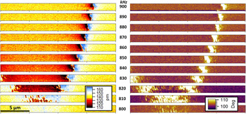
To monitor the dynamic response of the MEMS structure during in situ actuation, the same experimental configuration is used as above except an AC sinusoidal bias is applied to the electrodes that sandwich the piezoelectric film embedded in the suspended active cantilever. The tip, riding on the piezoactuating surface akin to Fig. 2(a) with the TF tine, is then scanned in a 20 by 1.25 µm swath (16:1 aspect ratio) of the MEMS lever as for Fig. 8. This is repeated 11 times in the same area, each with a distinct ac frequency of actuation of the MEMS structure similar to Fig. 5, in this case from 800 to 900 kHz in steps of 10 kHz with 3 V_ac. The ac-deflection of the AFM lever is analyzed with a lock-in-amplifier, just as with Fig. 2(b), and recorded during imaging. Figure 9 presents the resulting montage of AC amplitude (left) and phase (right) images for the MEMS structure in this nearly megahertz frequency range.

FIG. 9.

Resonant nodes revealed in eleven maps of amplitude (left) and phase (right) of an actuating piezoelectric MEMS lever in the same 20 µm by 1.25 µm area, as a function of drive frequency between 800 kHz (base) and 900 kHz (top) with steps of 10 kHz between frames as labeled.

A node in the AC response is clearly apparent in the amplitude and phase data, located at approximately 16 μm during 900 kHz excitations but evidently shifting left with lower frequencies (down in the figure). To the left of the node the amplitude is weaker than to the right. The node itself exhibits a paired antipeak and peak. Near x = 0 μm, a second node becomes apparent at 830 kHz. Both nodes converge at approximately 810 kHz, with hardly any evidence of these nodes at 800 kHz where the lever response is almost uniform over the measured length.

The actual mode and harmonic excited in this frequency range is unknown for the particular MEMS structure imaged (but could be with laser Doppler vibrometry). Sophisticated modeling has been performed for similar devices, though, to consider the first and higher order modes and even leverage these modes for enhanced MEMS performance.^{Reference Pulskamp, Proie and Polcawich68} It is certainly the case that the nearly-megahertz frequencies measured are beyond the first harmonic of the first mode for the lever. Qualitatively similar results were separately observed in other frequency ranges. Furthermore, this experiment was repeated on adjacent, identically designed, but shorter or longer MEMS structures. As expected, the same nodes were no longer apparent, since they strongly depend on the geometry of the resonating device.

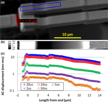
Finally, a T-shaped suspended lever as shown in Fig. 8(a) was actuated with voltage pulses instead of an AC sinusoidal signal. In addition to this actuating lever, though, there is also a pair of MEMS structures approaching from the opposite side, and in fact overhanging each half of the top of the ‘T’ shape (Fig. 10). Each is an independent electrode, such that the actuating MEMS device is designed to mechanically make or break electrical connections between the two contacts, by short circuiting them together from below if driven with sufficient voltage.^{Reference Proie, Polcawich, Pulskamp, Ivanov and Zaghloul29} The crossbar of the T-shape acts as the short circuiting element. AFM data were then acquired with the tip contacting one of these overhangs, allowing mapping of surface displacements in the slightly rotated area sketched at the right of Fig. 8(a). The oblique view secondary electron SEM image of Fig. 10(a), again with a rotated overlaid sketch of the AFM imaging region, clarifies the three-dimensionality of the lever and overhanging contacts. The tip scans from the end of the overhang (at left) to more than 10 μm away (at right).

FIG. 10.

SEM of T-shaped MEMS structure designed to electrically contact the two parallel electrodes at right by electromechanically actuating from below (a); AFM topography of one of the overhanging electrodes in the region sketched by a rotated rectangle (b) with equal lateral scaling as the SEM image; and AC vibration amplitude detected at the surface of the overhang due to periodic electromechanical contact from below with a range of pulse widths (c).

By design, the height of the overhanging structure is not uniform. This is evident in the SEM image, as well as the topography determined by the AFM, Fig. 10(b). Note that the lateral scales of these images (a and b) are matched for direct visual comparison.

The simultaneously acquired amplitude on the overhang is shown in Fig. 10(c), for pulse excitations ranging from 50 ns to 20 μs. These pulses repeated at a frequency of 25 kHz, with a magnitude (8 V) sufficient to cause the underlying T-shaped lever to strike the overhanging electrodes. The plot is presented with a log scale for the measured rms amplitude to more clearly reveal the various responses. Directly on the top of the electrode overhang, the rms amplitude of surface vibrations reaches as high as 15.7 nm, due to the repeated closing of the contact. Even for pulses of just 50 ns, though, measurable displacements are detected as far as 15 μm from the end of the overhanging structure, confirming coupling of the periodic mechanical contact many micrometers away from the contact point itself.

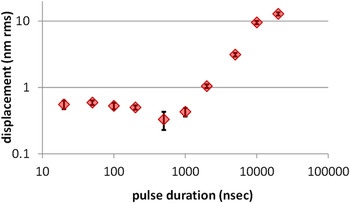
Focusing on a single position of a similar overhanging electrode, Fig. 11 plots the rms amplitude of surface displacements upon repeated contacts activated by voltage pulses with durations ranging over 3 orders of magnitude, from 20 ns to 20 μs. Taken alone, this result suggests a ∼5 μs pulse threshold, below which the MEMS structure does not substantially strike the overhang and hence the electrical contact may not be reliably made. This is compatible with electrical measurements of the relay signals from equivalent devices. Interestingly, though, the mapped AC response of the overhang structure in Fig. 10(c) shows that even 50 ns pulses generate a still-detectible surface displacement. In fact, reliable contact can be made in as fast as a few nanoseconds with more sophisticated MEMS designs.^{Reference Proie, Polcawich, Pulskamp, Ivanov and Zaghloul29} Future measurements will couple the relay signal with direct maps of the overhang displacement to elucidate the threshold pulse amplitudes and durations for reliable electrical contacts, and their correlations to displacements of the overhanging contacts. The ability to image the in situ response of such MEMS structures is therefore valuable for accurately investigating MEMS performance and reliability.

FIG. 11.

RMS amplitude of surface displacement for an overhanging contact struck by an underlying piezo-MEMS structure at a rate of 25 kHz, as a function of pulse duration.

It is reasonable to expect that the overall dynamic response of the MEMS structure will be sensitive to a combination of the strike rate as well as the impulse (applied force times the contact duration). The repeat rate here is fixed at 25 kHz (every 40 μs) regardless of the pulse dimensions, such that the results of Figs. 10(c) and 11 are for a fixed number of strikes in a given time, independent of the pulse shape. Therefore, the cumulative pulse time (i.e., the contacting time, reasonably assuming a 1:1 correlation) is smaller for the narrower pulses, perhaps contributing to the apparent turn-on behavior in Fig. 11. To normalize for this effect, similar measurements can of course be made that implement higher repeat rates for the shorter pulse durations. However, difficulties may arise since these different repeat rates can excite distinct modes or harmonics for the independent or coupled MEMS structures, including the AFM cantilever itself. As a result, the dynamics of the AFM lever itself could convolute the results, and therefore in this work a single frequency far from the AFM cantilever resonance is used.