



1 Introduction
Roughness affects many turbulent flows in engineering and in the natural sciences. At sufficiently high Reynolds number, in fact, any surface is rough, because the viscous length scale decreases with increasing Reynolds number, and eventually becomes comparable to the roughness length scale. Thus, understanding its effects is important to predict flow behaviours in most applications.
Roughness has been studied experimentally since the 1930s (Nikuradse Reference Nikuradse1933; Colebrook Reference Colebrook1939). Most of the work, however, has focused on equilibrium turbulent flows (flat-plate boundary layers, channels, pipes). Much less is known about the interaction between roughness and pressure gradients, especially adverse pressure gradients (APG) that cause separation. Every textbook discusses how roughness causes a decrease of the drag of bluff bodies, at fairly low Reynolds numbers, by causing early transition of the flow, thus delaying separation. The effect of roughness on separation in fully turbulent flows is the opposite: separation occurs earlier when roughness is present (Song & Eaton Reference Song and Eaton2002; Aubertine, Eaton & Song Reference Aubertine, Eaton and Song2004). How separation occurs in rough-wall boundary layers, compared with the smooth-wall case, is not known in great detail and many questions are still unanswered.
In the following literature review, we will summarize separately the work on roughness, separating boundary layers with a smooth wall and the combined effects of pressure gradient and roughness. Some of the important questions will be outlined, and the framework for this paper will be presented.
1.1 Canonical boundary layers with roughness
Reviews of the experimental findings on the effects of roughness in turbulent boundary layers (TBLs) can be found in Raupach, Antonia & Rajagopalan (Reference Raupach, Antonia and Rajagopalan1991) and Jiménez (Reference Jiménez2004). Over the last 15 years numerical simulations have also been able to contribute to the understanding of this phenomenon. Here we summarize the most important features. In TBLs under zero-pressure-gradient (ZPG), the surface roughness increases the drag exerted on the fluid. The momentum deficit due to roughness can be characterized by the roughness function
 $\unicode[STIX]{x0394}U^{+}$
, a downward shift of the mean velocity profile in the log-law region. Roughness determines the drag, therefore setting the velocity scale
 $u_{\unicode[STIX]{x1D70F}}=(\unicode[STIX]{x1D70F}_{w}/\unicode[STIX]{x1D70C})^{1/2}$
(where
 $\unicode[STIX]{x1D70F}_{w}$
is the wall stress and
 $\unicode[STIX]{x1D70C}$
the fluid density). Many velocity statistics, when normalized by
 $u_{\unicode[STIX]{x1D70F}}$
, are found to be unaffected by roughness outside of a layer of thickness
 $3{-}5k$
, where
 $k$
is the roughness height (Raupach et al.
Reference Raupach, Antonia and Rajagopalan1991; Flack, Schultz & Shapiro Reference Flack, Schultz and Shapiro2005; Kunkel, Allen & Smits Reference Kunkel, Allen and Smits2007).
Roughness also changes the mechanisms of production, diffusion and energy transfer between the mean and the turbulent fields, especially in the near-wall region. Krogstad, Antonia & Browne (Reference Krogstad, Antonia and Browne1992) and Krogstad & Antonia (Reference Krogstad and Antonia1999), for example, have observed the increase in wall-normal fluctuations near the wall. Shafi & Antonia (Reference Shafi and Antonia1995), among others, have reported the decreased anisotropy of the Reynolds stresses. Raupach et al. (Reference Raupach, Antonia and Rajagopalan1991) and Finnigan (Reference Finnigan2000) have shown that roughness causes a new production mechanism for the turbulent kinetic energy (TKE), the wake production, because of the spatial variations of the time-averaged velocity. Yuan & Piomelli (Reference Yuan and Piomelli2014b ), using direct numerical simulations of plane channel flow, showed that the wake production plays an important role in the Reynolds stress budgets: the wake production promotes wall-normal and spanwise fluctuations, contributing to the decrease of the Reynolds stress anisotropy observed by many researchers.
Most studies of roughness effects have been carried out in plane channel flows or ZPG boundary layers. Fewer investigations have examined flows out of equilibrium, and especially separating flows. However, flow separation occurs often in practical applications, and remains a challenge for turbulence models. The effects of roughness on the separation caused by an APG can be expected to be significant. While roughness-induced transition can be beneficial, delaying the separation, in turbulent boundary layers roughness affects the near-wall velocity, generally causing a momentum deficit that has the opposite effect.
1.2 Pressure-induced separating boundary layer
A geometry that has been used frequently, both in numerical and experimental studies, to investigate pressure-induced separation is the boundary layer on a flat plate, in which a tailored diverging–converging roof causes an APG followed by a steep favourable pressure gradient (FPG) that causes the flow to reattach (Perry & Fairlie Reference Perry and Fairlie1975; Patrick Reference Patrick1987; Mohammed-Taifour et al. Reference Mohammed-Taifour, Schwaab, Pioton and Weiss2015). A closed separation bubble is formed. In numerical experiments, blowing and suction at the free stream can be used to reproduce this effect (Spalart & Coleman Reference Spalart and Coleman1997; Na & Moin Reference Na and Moin1998; Skote & Henningson Reference Skote and Henningson2002; Cheng, Pullin & Samtaney Reference Cheng, Pullin and Samtaney2015). In this geometry the effects of pressure gradient can be separated from those of streamline curvature, making it an ideal test bed for the study of the effects of APG alone.
A number of separation characteristics have been investigated. One critical topic is the definition of separation itself. The locations of vanishing wall stress and mean flow reversal (the mean streamline detachment) have been extensively used as criteria of separation in two-dimensional flows. The actual separation, however, rarely happens at a single streamwise location but spreads over a region. Flow separation is now viewed as a process, rather than a localized event. Sandborn & Kline (Reference Sandborn and Kline1961) first defined the term ‘intermittent separation’ that indicates the onset of separation by the occurrence of intermittent backflow. Experiments (Simpson & Chew Reference Simpson and Chew1981; Dengel & Fernholz Reference Dengel and Fernholz1990; Alving & Fernholz Reference Alving and Fernholz1995) and simulations (Na & Moin Reference Na and Moin1998) suggest that the location where the instantaneous reversed flow occurs approximately 50 % of the time corresponds to the position where the averaged skin friction is zero. The change of backflow intermittency can start far ahead of flow separation. Vinuesa, Örlü & Schlatter (Reference Vinuesa, Örlü and Schlatter2017) studied attached flow over the suction side of a wing. The APG increase the occurrence of the backflow and especially the most extreme events. Large spanwise velocity fluctuations appear in the backflow at low APG and progressively decreases as the flow approaches separation. An open question is the validity of the intermittency criterion when additional factors other than the pressure gradient affect the near-wall flow: the intermittency of the near-wall turbulence can be modified in such situations.
In terms of the mean flow, the most recognizable feature of a wall-bounded flow under APG is the amplified wake of the mean velocity profile. Krogstad & Skare (Reference Krogstad and Skare1995), Skote & Henningson (Reference Skote and Henningson2002) and Nagib & Chauhan (Reference Nagib and Chauhan2008) (among others) have shown a consistent increase of the mean velocity relative to
 $u_{\unicode[STIX]{x1D70F}}$
in the wake region with pressure gradient. Monty, Harun & Marusic (Reference Monty, Harun and Marusic2011) reported that the wake region begins closer to the wall, reducing the extent of the logarithmic-law region with increasing APG. Much effort has been put into characterizing the mean velocity profile during flow separation, for the purpose of developing turbulent models. Several researchers tried to use a single velocity scale, letting the velocity profiles depend on the local pressure gradient and Reynolds number. Simpson & Stickland (Reference Simpson and Stickland1977), for instance, concluded that the canonical logarithmic law of the wall, in which the friction velocity is used as the velocity scale, holds until the location of intermittent separation. Note that such location can be far upstream of the point where the streamline detachment actually occurs. In other studies (Stratford Reference Stratford1959; Skote & Henningson Reference Skote and Henningson2002) a velocity scale based on pressure gradient is defined as
 $u_{p}=[(\unicode[STIX]{x1D708}/\unicode[STIX]{x1D70C})\;\text{d}P/\text{d}x]^{1/3}$
, where
 $\unicode[STIX]{x1D708}$
is the fluid kinematic viscosity and
 $\text{d}P/\text{d}x$
the streamwise pressure gradient. Despite extensive testing over various levels of pressure gradient and Reynolds numbers, however, no conclusive evidence supporting this approach, when the flow deviates significantly from the equilibrium state, has been obtained. Note that it has been demonstrated that the only strictly equilibrium wall-bounded flow over a smooth wall is the sink flow (Rotta Reference Rotta1962; Jones, Marusic & Perry Reference Jones, Marusic and Perry2001). A more relaxed definition of equilibrium is that the mean velocity exhibits self-similarity (Marusic et al.
Reference Marusic, McKeon, Monkewitz, Nagib, Smits and Sreenivasan2010), which is still very hard to maintain when the flow is under strong APG and approaching separation. It has been reported that in order to have a nearly equilibrium self-similar TBL under APG, the velocity at the free stream must follow a power law (Kitsios et al.
Reference Kitsios, Atkinson, Sillero, Borrell, Gungor, Jiménez and Soria2016; Bobke et al.
Reference Bobke, Vinuesa, Örlü and Schlatter2017). Kitsios et al. (Reference Kitsios, Atkinson, Sillero, Borrell, Gungor, Jiménez and Soria2016) showed that the outer scales can collapse the statistics in self-similar TBL for which the non-dimensional pressure gradient is constant. Coles (Reference Coles1956) and Perry & Schofield (Reference Perry and Schofield1973), among others, tried to make the profiles collapse onto a single curve in an outer scaling. In such methods, velocity profiles at streamwise positions close to the separation point can only be made to collapse in the outer part through a fitting procedure of the velocity scale. One of the most satisfactory scalings seems to be the empirical one proposed by Zagarola & Smits (Reference Zagarola and Smits1998) for fully developed pipe flow. The outer velocity scale was proposed to be
 $U_{\infty }\unicode[STIX]{x1D6FF}^{\ast }/\unicode[STIX]{x1D6FF}$
, where
 $\unicode[STIX]{x1D6FF}^{\ast }$
is the displacement thickness and
 $\unicode[STIX]{x1D6FF}$
the boundary layer thickness. Because of the use of the
 $\unicode[STIX]{x1D6FF}^{\ast }/\unicode[STIX]{x1D6FF}$
factor, the parameter space is reduced, leading to possible self-similar states. This type of scaling has been proved to work even for very strong APG (Castillo, Wang & George Reference Castillo, Wang and George2004; Maciel, Rossignol & Lemay Reference Maciel, Rossignol and Lemay2006; Materny et al.
Reference Materny, Drozdz, Drobniak and Elsner2008; Vinuesa et al.
Reference Vinuesa, Bobke, Örlü and Schlatter2016).
The APG also has significant effects on the Reynolds stresses. Krogstad & Skare (Reference Krogstad and Skare1995) showed that strong APG reduces the anisotropy of the near-wall turbulence; the fourth quadrant events become dominant. This result agrees with the observations by Skote & Henningson (Reference Skote and Henningson2002), Lee & Sung (Reference Lee and Sung2009) and others that the near-wall streaks are weaker in strong APG TBL. An outer peak in the form of a broad and flat hump highlights the changes in the stresses due to APG. The significant production of TKE at such location is related to the peak in the Reynolds shear stresses there (Skare & Krogstad (Reference Skare and Krogstad1994), Lee & Sung (Reference Lee and Sung2008) among others). So far no scaling has been found to collapse the Reynolds stress profiles in APG TBLs (Drozdz & Elsner Reference Drozdz and Elsner2011). The scaling proposed by Zagarola & Smits (Reference Zagarola and Smits1998) for the mean velocity, for instance, does not give satisfactory results for the Reynolds stresses. For APG TBLs in which a closed separation bubble is formed, the amplified Reynolds stresses in the detached shear layer attenuate near the top of the separation bubble, and a negative production region of the TKE appears when the streamline reaches its most convex point (Spalart & Coleman Reference Spalart and Coleman1997; Skote & Henningson Reference Skote and Henningson2002; Abe et al. Reference Abe, Mizobuchi, Matsuo and Spalart2012). Abe et al. (Reference Abe, Mizobuchi, Matsuo and Spalart2012) emphasized that this type of negative production is caused by the direct effects of APG on the anisotropic large scales, instead of following a reduction in dissipation at the small scales.
The secondary peak in Reynolds stress profiles indicates the importance of the outer layer in APG TBLs, where the large-scale turbulent motions are dominant. Large-scale streamwise-elongated eddies are generated in the outer layer (Lee & Sung Reference Lee and Sung2009; Rahgozar & Maciel Reference Rahgozar and Maciel2011) similar to the ones observed in the overlap region in ZPG TBLs. Other researcher described the structures as a streamwise series of organized hairpin vortices (instead of randomly distributed ones as in the ZPG TBL) (Adrian, Meinhart & Tomkins Reference Adrian, Meinhart and Tomkins2000; Ganapathisubramani, Longmire & Marusic Reference Ganapathisubramani, Longmire and Marusic2003). These structures were also identified as the source of the oscillation of the separation bubble (Na & Moin Reference Na and Moin1998; Kaltenbach et al.
Reference Kaltenbach, Fatica, Mittal, Lund and Moin1999; Mohammed-Taifour & Weiss Reference Mohammed-Taifour and Weiss2016) and the unsteadiness of the beginning of the separation bubble (Simpson & Chew Reference Simpson and Chew1981; Na & Moin Reference Na and Moin1998; Cheng et al.
Reference Cheng, Pullin and Samtaney2015). A direct numerical simulation (DNS) study performed by Lee & Sung (Reference Lee and Sung2009) demonstrated that the swirling motion due to each individual hairpin in the outer region is stronger for the APG flow than for the ZPG flow. The legs of the hairpin vortices, in the log layer, are more inclined in the APG cases. Beyond the logarithmic layer, the backbone of the steeply inclined part of each eddy has a
 $\unicode[STIX]{x1D6EC}$
shape that does not change when normalized by the boundary layer thickness. Drozdz & Elsner (Reference Drozdz and Elsner2011) used bursting process analysis in their experiments to detect the large-scale structures. They showed that the continuous growth of trajectory inclination of eddies associated with the hairpin vortices, which is consistent with the results reported by Lee & Sung (Reference Lee and Sung2009), leads to the appearance of the secondary peak in the Reynolds stresses in the outer layer. Monty et al. (Reference Monty, Harun and Marusic2011) conducted experiments in an expanding wind tunnel and demonstrated that the large-scale structures are more energized by the pressure gradient in the outer region than the small-scale ones. Rahgozar & Maciel (Reference Rahgozar and Maciel2011) examined the APG TBLs by measuring the turbulence field at several wall-normal and streamwise locations to explore the variations of the structures. They found that the APG leads to a less frequent appearance of these large structures, especially in the lower part of the TBL near separation. Recently Maciel, Gungor & Simens (Reference Maciel, Gungor and Simens2017) found that the wall-attached structures below
 $y/\unicode[STIX]{x1D6FF}=0.2$
lose their streamwise elongation, and the detached ones in the middle of the TBL (
 $y/\unicode[STIX]{x1D6FF}=0.3{-}0.7$
) are less changed than the near-wall ones. Kitsios et al. (Reference Kitsios, Atkinson, Sillero, Borrell, Gungor, Jiménez and Soria2016) examined the two-point correlation at the distance of displacement thickness in a TBL subjected to APG and also reported the structures becomes shorter in the streamwise direction.
1.3 Combined effects of APG and roughness
Much less attention has been paid to the flow over rough surface subjected to free-stream pressure gradient, especially when the APG is strong enough to induce flow separation. Some experimental studies focused on the mild APG effects on roughness, in particular, the roughness function (Perry & Joubert Reference Perry and Joubert1969; Pailhas, Touvet & Aupoix Reference Pailhas, Touvet and Aupoix2008; Tay, Kuhn & Tachie Reference Tay, Kuhn and Tachie2009; Tsikata & Tachie Reference Tsikata and Tachie2013; Shin & Song Reference Shin and Song2014). There is, however, a divergence of opinion on the combined effects of roughness and APG on the total drag, which may be due to the uncertainty in obtaining the wall stress in experiments. Also, the APG in these studies was relatively low, to maintain the logarithmic law of the velocity.
Song & Eaton (Reference Song and Eaton2002) and Aubertine et al. (Reference Aubertine, Eaton and Song2004) studied the separated flow over a ramp covered by sand paper. The ramp was smoothly contoured to avoid fixed-point separation due to geometry. Early separation was reported for the rough-wall case, due to the large mean momentum deficit near the rough wall. Substantially larger separation bubbles were found in comparison with the smooth-wall case. The normal Reynolds stresses were reported by Song & Eaton (Reference Song and Eaton2002) and Aubertine et al. (Reference Aubertine, Eaton and Song2004) to be less sensitive to the APG in rough-wall flows: dominant peaks near the surface appear in the smooth case when the flow is subjected to the APG, which turned into a wider bump throughout the boundary layer in the rough-wall case, owing to enhanced mixing. A weaker ejection and stronger sweep contribution to the Reynolds shear stress up to the location of flow separation was also reported, which agrees with the APG effects on Reynolds shear stress contribution but differs from the roughness effects reported in previous studies: Krogstad et al. (Reference Krogstad, Antonia and Browne1992) in their experiments of ZPG TBL over roughness reported that both the ejection and sweep events are stronger due to roughness. Schultz & Flack (Reference Schultz and Flack2007) performed experiments with significantly large
 $\unicode[STIX]{x1D6FF}/k$
ratio, where
 $k$
is the roughness height, and reported the same contributions to the Reynolds shear stress in the smooth- and rough-wall TBLs. They also found that near the wall, strong (
 $|u^{\prime }v^{\prime }|>5|\langle u^{\prime }v^{\prime }\rangle |$
, where
 $u^{\prime }$
and
 $v^{\prime }$
are the velocity fluctuations in the streamwise and wall-normal directions, and
 $\langle \cdot \rangle$
represents the Reynolds average) ejection decreases and strong sweep increases. The combined effects of APG and roughness on the contribution of the sweep and ejection are still not clear.
A difference between the studies by Song & Eaton (Reference Song and Eaton2002) and Aubertine et al. (Reference Aubertine, Eaton and Song2004) and those on smooth-wall APG TBL is the existence of the mild surface curvature in those studies. Also, due to the limitations of the experimental instruments, the friction velocity was determined by extrapolating the total shear stress above the roughness; the possible uncertainty was emphasized. Moreover, the measurements did not extend to the trough of the roughness elements.
1.4 Objectives
The present work attempts to shed light on these issues by carrying out large-eddy simulations (LES) of the TBL on a flat plate with a rough surface, subjected to strong APG. The flow configuration uses suction and blowing at the free stream of the TBL, as in previous numerical studies (Na & Moin Reference Na and Moin1998). The Reynolds number based on the momentum thickness and free-stream velocity at the reference plane,
 $Re_{\unicode[STIX]{x1D703},o}=U_{o}\unicode[STIX]{x1D703}_{o}/\unicode[STIX]{x1D708}$
is 2,500. This value of
 $Re$
is much larger than that in previous simulations (which ranged between 300 (Na & Moin Reference Na and Moin1998) and 1000–1400 (Lee & Sung Reference Lee and Sung2009)). It allows the flow to be in the fully rough regime in the attached TBL while maintaining a roughness height much smaller than the boundary layer thickness. Our focus is on the separation point itself, and on the differences in the dynamics of flow separation between the smooth-wall and rough-wall cases. In the following, we first review the numerical methodology, and then discuss the flow development, as well as the mean flow features; we then compare various separation criteria, and finally describe roughness effects on Reynolds stresses. Finally we draw the main conclusions and make recommendations for future work.
2 Problem formulation
In LES the filtered equations of conservation of mass and momentum are solved; in incompressible flow they are:
 $$\begin{eqnarray}\displaystyle & \displaystyle \unicode[STIX]{x1D735}\boldsymbol{\cdot }\overline{\boldsymbol{u}}=0, & \displaystyle\end{eqnarray}$$
 $$\begin{eqnarray}\displaystyle & \displaystyle \frac{\unicode[STIX]{x2202}\overline{\boldsymbol{u}}}{\unicode[STIX]{x2202}t}+\overline{\boldsymbol{u}}\boldsymbol{\cdot }\unicode[STIX]{x1D735}\overline{\boldsymbol{u}}=-\unicode[STIX]{x1D735}\overline{p}-\unicode[STIX]{x1D735}\boldsymbol{\cdot }\unicode[STIX]{x1D749}+\frac{1}{Re}\unicode[STIX]{x1D6FB}^{2}\overline{\boldsymbol{u}}+\boldsymbol{f}. & \displaystyle\end{eqnarray}$$
An overline denotes the spatial filtering operation and
 $\unicode[STIX]{x1D70F}_{ij}=\overline{u_{i}u}_{j}-\overline{u}_{i}\overline{u}_{j}$
are the sub-filter stresses (SFS) modelled by the integral length scale approximation (ILSA) model (Piomelli, Rouhi & Geurts Reference Piomelli, Rouhi and Geurts2015) in its local form (Rouhi, Piomelli & Geurts Reference Rouhi, Piomelli and Geurts2016). A value of
 $s_{\unicode[STIX]{x1D70F}}=0.02$
was chosen as a measure of the SFS activity.
 $x_{i}$
,
 $i=1$
, 2 and 3 (or
 $x$
,
 $y$
and
 $z$
) are streamwise, wall-normal and spanwise directions, respectively, and
 $f_{i}$
is the body force term used in the immersed boundary method to represent the roughness elements (see below). Reference velocity and length scales are used to make the equations dimensionless and define the Reynolds number; they will be specified momentarily.
Computational domain. Sand grain roughness for the rough-wall case is visualized by the iso-surfaces of
 $\unicode[STIX]{x1D719}=0.5$
(the fraction of each grid cell volume occupied by the fluid), coloured by the roughness height. The zoomed-in view in the lower-right corner shows the start of the roughness patch. The inset in the upper-left corner shows the mean profile of
 $\unicode[STIX]{x1D719}$
in the wall-normal direction.

The computational domain is shown in figure 1. The scales used for normalization are the free-stream velocity,
 $U_{o}=U_{\infty }(x=0)$
, and the momentum thickness,
 $\unicode[STIX]{x1D703}_{o}=\unicode[STIX]{x1D703}(x=0)$
, at a reference plane in the ZPG region. The recycling and rescaling method of Lund, Wu & Squires (Reference Lund, Wu and Squires1998) together with the random dynamic spanwise shift proposed by Morgan et al. (Reference Morgan, Larsson, Kawai and Lele2011), is used at the inlet, while a convective boundary condition (Orlanski Reference Orlanski1976) is used for the outlet. The recycling region ranges from
 $x=-100$
to
 $-50~\unicode[STIX]{x1D703}_{o}$
.
On the bottom wall, an immersed boundary method based on the volume-of-fluid approach is used to impose the no-slip conditions on the roughness surface (Scotti Reference Scotti2006). The roughness used here is a virtual sand paper constructed from randomly oriented and distributed ellipsoids of the same shape and size. The bottom wall was partitioned into square tiles of size
 $2k$
; the centre of a randomly oriented ellipsoid with semiaxes
 $k$
,
 $1.4k$
and
 $2k$
is placed at a random location within each tile at
 $y=-0.5k$
. The volume fraction of each grid cell occupied by the fluid,
 $\unicode[STIX]{x1D719}$
, is calculated in pre-processing. The implementation of the immersed boundary method (i.e. the determination of the value of
 $f_{i}$
in (2.2)), is described in Yuan & Piomelli (Reference Yuan and Piomelli2014a
). A brief summary is provided in the appendix A. The surface
 $\unicode[STIX]{x1D719}=0.5$
(representative of the shape of the rough wall) is shown in the figure. Notice that the roughness patch starts downstream of the recycling plane and the roughness height increases linearly from 0 to
 $k$
over
 $12\unicode[STIX]{x1D703}_{o}$
, so that the recycling/rescaling procedure can be implemented on a smooth surface. A similar roughness transition is also used near the outlet. The roughness height is
 $k=0.715\unicode[STIX]{x1D703}_{o}$
. The mean height for such surface is
 $\overline{k}=0.6k\approx 0.42\unicode[STIX]{x1D703}_{o}$
, and the roughness crest is at
 $y=1.5k$
(when one ellipsoid rotates and the longest axis lays in the vertical direction, the end point has the largest distance to the surface
 $2k-0.5k=1.5k$
). The mean
 $\unicode[STIX]{x1D719}$
profile in the wall-normal direction is shown in the figure. Note that the virtual wall in the rough-wall case (i.e. the location of the centroid of the local force profile) is at
 $d=0.8k$
(for details on the calculation of
 $d$
refer to the appendix A and Yuan & Piomelli (Reference Yuan and Piomelli2014a
)). The chosen roughness height ensures significant roughness effects, while not significantly blocking the boundary layer (we have
 $\unicode[STIX]{x1D6FF}/\overline{k}\geqslant 15$
).
Simulation parameters.
 $N_{i}$
is the number of grid points in the entire domain,
 $n_{i}$
the number of grid points per sand grain element.

At the upper boundary the vertical velocity profile
 $V_{top}$
is assigned; after a ZPG region, a suction zone is present, followed by blowing and by another ZPG region near the outlet. The normal derivative of the streamwise velocity satisfies the zero mean vorticity condition, and the one of the spanwise velocity is zero. Periodic boundary conditions are used in the spanwise direction, and a no-slip condition at the wall in the smooth case. When roughness is used, the immersed boundary method described above is used to set the velocity to zero on and inside the roughness elements. The calculation domain is
 $L_{x}\times L_{y}\times L_{z}=570\unicode[STIX]{x1D703}_{o}\times 70\unicode[STIX]{x1D703}_{o}\times 54\unicode[STIX]{x1D703}_{o}$
for both cases. The total length of the roughness patch is
 $480\unicode[STIX]{x1D703}_{o}$
. Reynolds numbers and grid resolutions are listed in table 1. A uniform grid is employed in the streamwise and spanwise direction, and a stretched grid in the wall-normal direction. In the rough-wall case, constant
 $\unicode[STIX]{x0394}y/\unicode[STIX]{x1D703}_{o}=4\times 10^{-3}$
is used below
 $1.5k$
, which significantly increases the total number grid points in the wall-normal direction compared with the smooth-wall one. The grid is also clustered in the wall-normal direction near the upper boundary. The present grid sizes in wall units (wall units are obtained using the friction velocity at the reference location,
 $u_{\unicode[STIX]{x1D70F},o}$
as the velocity scale) are comparable to the values used in other LES studies on separating TBL (Fröhlich et al.
Reference Fröhlich, Mellen, Rodi, Temmerman and Leschziner2005). Compared with the Kolmogorov scale
 $\unicode[STIX]{x1D702}$
, the present resolution gives
 $\unicode[STIX]{x0394}x/\unicode[STIX]{x1D702}\leqslant 7$
,
 $\unicode[STIX]{x0394}z/\unicode[STIX]{x1D702}\leqslant 5$
and
 $\unicode[STIX]{x0394}h/\unicode[STIX]{x1D702}\leqslant 6$
(where
 $\unicode[STIX]{x0394}h=(\unicode[STIX]{x0394}x^{2}+\unicode[STIX]{x0394}y^{2}+\unicode[STIX]{x0394}z^{2})^{1/2}$
). Since the maximum dissipation occurs at a length scale of approximately
 $24\unicode[STIX]{x1D702}$
(Pope Reference Pope2000), the present grid is able to resolve a substantial part of the dissipation spectrum. The maximum SFS viscosity is less than three times the molecular one in the separated shear layer, and less than the molecular viscosity in the attached regions. For the smooth case, a grid with half the nodes in the wall-parallel plane shows less than 1 % difference in the mean velocity and Reynolds stresses, showing that the calculation is grid converged. Furthermore, the current grids are sufficient to represent the random shape of roughness elements and the flow structures developed around them: although the shape of the ellipsoids is not reproduced in detail, this model was shown to represent the effects of randomly distributed roughness. Yuan & Piomelli (Reference Yuan and Piomelli2014a
) showed that, as long as at least four points are used in each wall-parallel direction, the drag and the wake field statistics converge. In the present case we use 6 points in
 $x$
, and 10 in
 $z$
.
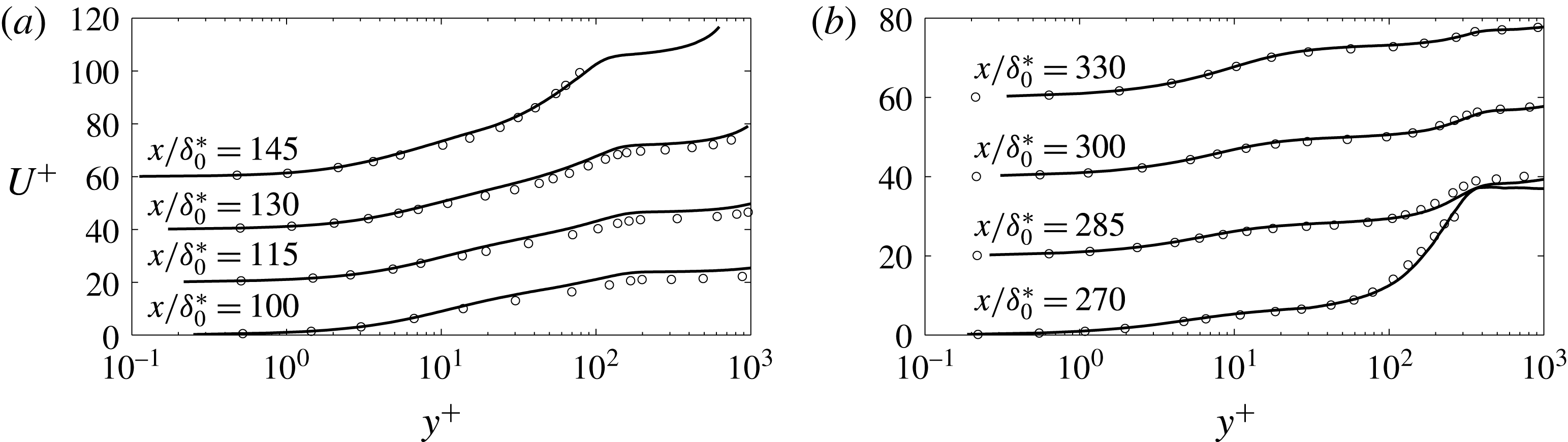
Profiles of the mean streamwise velocity before (a) and after (b) separation. —— LES, ○ DNS by Na & Moin (Reference Na and Moin1998). Each profile is shifted upward by 20 units for clarity.
The simulations were performed using a well-validated code (Keating et al.
Reference Keating, Piomelli, Bremhorst and Nešić2004) that solves equations (2.1)–(2.2) on a staggered grid. A second-order accurate central differencing scheme was used for all the spatial terms. A second-order accurate semi-implicit time advancement method was employed in which the Crank–Nicolson scheme is used for the wall-normal diffusive terms, while the Adams–Bashforth scheme is applied to the remaining ones. The statistical data were sampled at equal time interval,
 $\unicode[STIX]{x0394}t=5.0\unicode[STIX]{x1D703}_{o}/U_{o}$
, once statistically steady state was reached. The total averaging time was
 $T=750\unicode[STIX]{x1D703}_{o}/U_{o}$
for the rough-wall case and
 $T=1200\unicode[STIX]{x1D703}_{o}/U_{o}$
for the smooth-wall one. The mean velocity obtained using only half of the sample was within 1 % of that calculated using the entire sample. In the following discussion, the averaged quantities will be denoted as capital letters for primary flow variables, and by
 $\langle \cdot \rangle$
for turbulent statistics.
The present computational settings are validated by comparison with the DNS case of Na & Moin (Reference Na and Moin1998), at a lower Reynolds number. The velocity profiles in wall coordinates are shown in figure 2, and the agreement is very good. A comparison of the Reynolds stress contours with those in figure 22 in Na & Moin (Reference Na and Moin1998) also shows satisfactory agreement (not shown). Some minor discrepancies may be due to the sensitivity of contours to sampling size and other factors, which makes an exact quantitative comparison difficult.
3 Results
3.1 Flow development
The profiles representing the development of the boundary layer are shown in figure 3. The acceleration parameter,
 $$\begin{eqnarray}\displaystyle & \displaystyle K=\frac{\unicode[STIX]{x1D708}}{U_{\infty }^{2}}\frac{\text{d}U_{\infty }}{\text{d}x}, & \displaystyle\end{eqnarray}$$
where
 $U_{\infty }$
is the time- and spanwise-averaged free-stream velocity, is almost zero for
 $x/\unicode[STIX]{x1D703}_{o}\leqslant 50$
(figure 3
b). In this region a standard ZPG behaviour is observed for the boundary layer growth (figure 3
c,d). This region will be referred to as the ‘ZPG region’ hereafter.
Profiles of: (a)
 $U_{top}$
; (b) acceleration parameter
 $K$
; (c)
 $Re_{\unicode[STIX]{x1D703}}$
; (d)
 $\unicode[STIX]{x1D6FF}$
. —— smooth wall; - - - rough wall; – - – in (a)
 $V_{top}$
; – - – in (d)
 $\unicode[STIX]{x1D6FF}=0.37xRe_{x}^{-1/5}$
.

Mean pressure coefficients
 $C_{p}$
. —— smooth wall, - - - rough wall. Lines only, at the wall for the smooth wall and at
 $(y-d)/\unicode[STIX]{x1D703}=0.5$
for the rough; lines with circle mark,
 $(y-d)/\unicode[STIX]{x1D703}_{o}=15$
; lines with triangle mark,
 $y=L_{y}$
. The reference pressure is obtained at the top boundary at the reference streamwise location.

The mean pressure coefficient
 $$\begin{eqnarray}\displaystyle & \displaystyle C_{p}=\frac{P-P_{o}}{\unicode[STIX]{x1D70C}U_{o}^{2}/2} & \displaystyle\end{eqnarray}$$
is shown in figure 4. We compare its value at the wall in the smooth-wall case, and at
 $(y-d)=0.7k=0.5\unicode[STIX]{x1D703}_{o}$
(i.e. the roughness crest) for the rough-wall one. We also consider its value at
 $(y-d)=15\unicode[STIX]{x1D703}_{o}$
(a line corresponding to the maximum boundary layer thickness in the attached flow region), and at the top boundary. The profiles show that the streamwise pressure gradient is uniform in the boundary layer, although quite different from that imposed at the top boundary. The pressure gradient experienced by the flow is adverse up to
 $x\simeq 150\unicode[STIX]{x1D703}_{o}$
, nearly zero up to
 $250\unicode[STIX]{x1D703}_{o}$
and favourable through the rest of the useful region. The pressure gradient imposed at the free stream, on the other hand, alternates several regions of FPG and APG. From here on, the region up to
 $x\simeq 150\unicode[STIX]{x1D703}_{o}$
will be referred to as the ‘APG region’.
The deceleration causes the boundary layer to thicken rapidly downstream of
 $x/\unicode[STIX]{x1D703}_{o}=50$
, and
 $Re_{\unicode[STIX]{x1D703}}=U_{e}\unicode[STIX]{x1D703}/\unicode[STIX]{x1D708}$
to increase (
 $U_{e}$
is the free-stream velocity at the boundary layer edge). Notice that the definition of the boundary layer edge is non-trivial in APG TBLs because the velocity at the edge is ill defined. Here the ‘diagnostic plot’ method (Alfredsson, Segalini & Örlü Reference Alfredsson, Segalini and Örlü2011; Vinuesa et al.
Reference Vinuesa, Bobke, Örlü and Schlatter2016) is employed to obtain
 $\unicode[STIX]{x1D6FF}$
(figure 3
c). In their study Vinuesa et al. (Reference Vinuesa, Bobke, Örlü and Schlatter2016) proved that this method is valid over a wide range of pressure gradients
 $0<\unicode[STIX]{x1D6FD}<85$
, where
 $\unicode[STIX]{x1D6FD}$
is the Clauser pressure-gradient parameter
 $$\begin{eqnarray}\displaystyle & \displaystyle \unicode[STIX]{x1D6FD}=\frac{\unicode[STIX]{x1D6FF}^{\ast }}{\unicode[STIX]{x1D70C}u_{\unicode[STIX]{x1D70F}}^{2}}\frac{\text{d}P_{e}}{\text{d}x} & \displaystyle\end{eqnarray}$$
in which
 $\unicode[STIX]{x1D6FF}^{\ast }$
is the displacement thickness and
 $P_{e}$
is the pressure at the boundary layer edge; in the present case,
 $1<\unicode[STIX]{x1D6FD}<50$
upstream of the separation bubble before
 $u_{\unicode[STIX]{x1D70F}}$
goes below
 $0.01U_{e}$
.
Profiles of the skin-friction coefficient. —— smooth wall; - - - rough wall; lines with marker Clauser pressure-gradient parameter
 $\unicode[STIX]{x1D6FD}$
for the attached flow. Grey regions show the root-mean-square range of
 $C_{f}$
in the two cases.
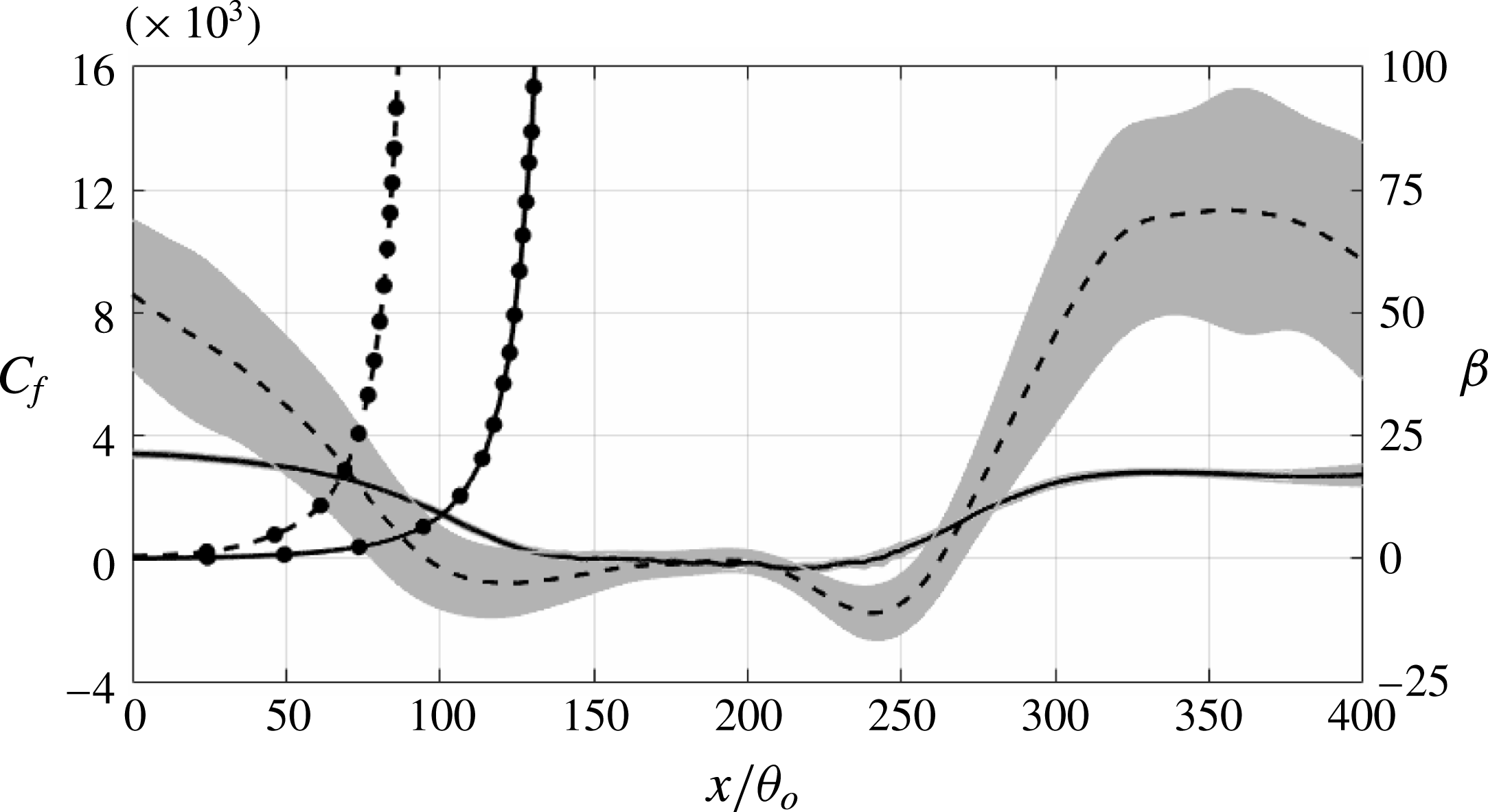
Figure 5 shows the skin-friction coefficient,
 $C_{f}=2\unicode[STIX]{x1D70F}_{w}/\unicode[STIX]{x1D70C}U_{o}^{2}$
, and
 $\unicode[STIX]{x1D6FD}$
before flow separation. For the rough surface,
 $C_{f}$
is based on the total drag exerted by the surface on the fluid. This drag can be calculated from the conservation of the streamwise momentum, or as the integral of the
 $f_{u}$
term in (2.2) throughout the roughness layer (
 $y\leqslant 1.5k$
) (for details, refer to Yuan & Piomelli Reference Yuan and Piomelli2014a
). It is important to note that in the immersed boundary method with volume-of-fluid approach used here, the body force includes both the viscous drag and the form drag induced by the roughness. The highlighted range indicates the root-mean-square (r.m.s.)
 $C_{f}$
at corresponding location. When
 $C_{f}$
is obtained by averaging over the spanwise direction and time, if the number of roughness elements in the spanwise direction (i.e.
 $L_{z}/(2k)$
) is small, an oscillatory behaviour with scale 2
 $k$
is observed. It is due to wakes forming behind each roughness element which lead to local pressure gradients varying significantly with the spatial distribution of elements and the local flow field. If very few roughness elements are used in the spanwise direction, at some locations the stagnation points may be more numerous, giving rise to higher-than-average pressure, at others the wakes may be prevalent, giving lower-than-average pressure; this oscillation is reflected in the form drag. Given that the local pressure gradient is mainly due to the pressure difference across the roughness element, it is relatively stationary and cannot be removed by longer time averaging. Increasing the amount of randomly distributed roughness elements in the spanwise direction can lead to better ensemble averaging as the stagnation points and wakes average out, but at significant computational cost.
Yuan & Piomelli (Reference Yuan and Piomelli2014b
) showed that, in order to decrease the amplitude of these oscillations to 5 % of the mean
 $C_{f}$
, approximately 500 elements are necessary. In the current simulation, only 37 roughness elements are distributed along the spanwise direction, and the insufficient sample leads to highly fluctuating quantities, when averaged in the spanwise direction and time within the roughness region. Therefore, in the rough case we also average the wall stress over a window of
 $2k$
in the streamwise direction, and use spline fitting to smooth the profile. The same smoothing method is used in the following analysis in the rough-wall case for averaged quantities examined in the near-wall region. The r.m.s. is then calculated by the difference between the mean
 $C_{f}$
and the instantaneous ones averaged in the spanwise direction and time only. The r.m.s. can be viewed as a measure of the uncertainty due to the finite span of the domain, and is reported to show that the differences between smooth and rough-wall cases are well outside the uncertainty itself. We observe that
 $C_{f}$
becomes zero much earlier in the rough-wall case. This condition is usually considered to indicate flow separation, but in this case different phenomena are occurring, which will be discussed below in § 3.3.
3.2 Mean velocity
Contours of the mean streamwise velocity,
 $U(x,y)$
, are shown in figure 6. Streamlines, defined as contours of the streamfunction
 $$\begin{eqnarray}\displaystyle & \displaystyle \unicode[STIX]{x1D713}(x,y)=\int _{0}^{y}U(x,y^{\prime })\,\text{d}y^{\prime } & \displaystyle\end{eqnarray}$$
are superposed on the velocity contours. Since the roughness crest is at
 $(y-d)/\unicode[STIX]{x1D703}_{o}=0.5$
, we choose the streamline that passes the
 $U=0$
point at this height as the one quantifying the separation bubble. It will be referred to as
 $\unicode[STIX]{x1D713}_{o}$
hereafter. We observe a significant region of recirculating flow in both cases. The separation bubble is 78 % longer and 71 % thicker in the rough-wall case (
 $L_{s}/\unicode[STIX]{x1D703}_{o}=148$
,
 $H_{s}/\unicode[STIX]{x1D703}_{o}=22.2$
, compared with
 $L_{s}/\unicode[STIX]{x1D703}_{o}=83$
,
 $H_{s}/\unicode[STIX]{x1D703}_{o}=13.0$
in the smooth case). Such increase of the separation bubble size, and both earlier separation and later reattachment, were also reported in previous studies (Song & Eaton Reference Song and Eaton2002; Aubertine et al.
Reference Aubertine, Eaton and Song2004). Notice, however, that in the rough-wall case, the point where the mean velocity
 $U=0$
above the roughness crest, in figure 6(b), occurs significantly downstream of the point where
 $C_{f}=0$
; this issue will be discussed in § 3.3.
Contours of mean streamwise velocity normalized by
 $U_{o}$
. (a) Smooth wall, (b) rough wall. ——, streamlines at
 $\unicode[STIX]{x1D713}_{o}$
and
 $\unicode[STIX]{x1D713}/(U_{o}\unicode[STIX]{x1D703}_{o})=0.5$
, 1, 1.5 and 2.

Relatively strong mean backflow occurs in the rear part of both separation bubbles, while the front part shows a very weak flow reversal. This result agrees with previous studies showing that immediately downstream of the streamline detachment point, the fluid elements forming the weak mean backflow do not come from far downstream. Simpson (Reference Simpson1989, Reference Simpson1996) found that these fluid elements are generated intermittently by the large-scale turbulence in the separated boundary layer, and such region usually extends up to the location where the thickness of the separation bubble becomes comparable to the boundary layer thickness. In current simulations, the mean negative velocity in the separation bubble is significantly larger in the rough-wall case. In particular, the range of the backflow region far downstream of the detachment seems to persist, but the weak mean backflow region is enlarged at the leading edge of the separation bubble. This indicates that the momentum transport by the shear layer structures is amplified near the flow detachment region.
Profiles of: (a) mean streamwise velocity in wall units in the ZPG and mild APG regions. —— smooth wall, - - - rough wall. – - –
 $U^{+}=(1/0.41)\text{log}(y^{+})+5.0$
. Each profile is shifted upwards by 30 units for clarity; (b) roughness function at several streamwise locations (inset shows the log-law slope
 $\unicode[STIX]{x1D6F7}=1/(y^{+}\unicode[STIX]{x2202}U^{+}/\unicode[STIX]{x2202}y^{+})$
,
 $\unicode[STIX]{x0394}U^{+}$
is measured at
 $(y-d)^{+}=90$
). – ○ – present rough-wall case,
 $k_{s}=1.6k$
,
 $x/\unicode[STIX]{x1D703}_{o}$
increases from zero by step
 $2\unicode[STIX]{x1D703}_{o}$
from right to left; – - –
 $\unicode[STIX]{x0394}U^{+}=(1/0.41)\text{log}(k_{s}^{+})-3.5$
; (c) mean streamwise velocity in outer scale. —— smooth wall, - - - rough wall. Each profile is shifted to the right by one unit for clarity.
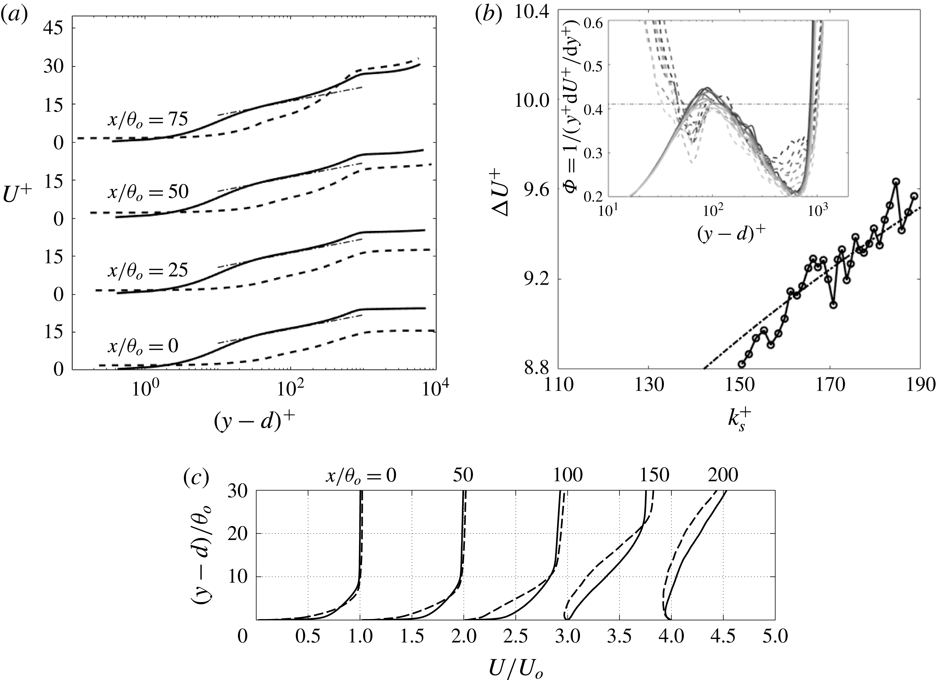
Figure 7(a) shows the mean streamwise velocity profiles in wall units upstream of the separation bubble. In the ZPG region the velocity profiles of both the smooth- and rough-wall cases show the logarithmic law, with different intercepts. Further downstream (not shown), the profiles rapidly deviate from logarithmic behaviour, and a large wake region appears. The wake region, which in the current flow starts to show from
 $x/\unicode[STIX]{x1D703}_{o}=75$
, is one of the most recognizable feature of an APG TBL (Clauser Reference Clauser1954). At
 $x/\unicode[STIX]{x1D703}_{o}=75$
, the rough-wall profile starts to deviate from the log law, while the smooth-wall profile remains logarithmic.
The downward shift of the log-law profiles, the ‘roughness function’
 $\unicode[STIX]{x0394}U^{+}$
, quantifies the momentum deficit due to roughness. In previous studies it was reported that
 $\unicode[STIX]{x0394}U^{+}$
depends on both the roughness Reynolds number,
 $k^{+}=ku_{\unicode[STIX]{x1D70F}}/\unicode[STIX]{x1D708}$
, and the surface texture (Nikuradse Reference Nikuradse1933; Colebrook Reference Colebrook1939; Raupach et al.
Reference Raupach, Antonia and Rajagopalan1991; Jiménez Reference Jiménez2004). The equivalent sand grain roughness height,
 $k_{s}$
, is used as a measure of the roughness size that is independent on the shape of the roughness elements. With the present sand grain model, for
 $k^{+}$
in the transitionally rough regime,
 $k_{s}\simeq k$
(Scotti Reference Scotti2006), whereas in the fully rough regime,
 $k_{s}\simeq 1.6k$
(Yuan & Piomelli Reference Yuan and Piomelli2014a
). The relation between
 $\unicode[STIX]{x0394}U^{+}$
and
 $k_{s}^{+}$
is shown in figure 7(b). Based on its definition (
 $\unicode[STIX]{x0394}U^{+}=1/\unicode[STIX]{x1D705}\log [(y-d)^{+}]+B-U^{+}$
, where
 $\unicode[STIX]{x1D705}=0.41$
and
 $B=5.0$
are log-law constants),
 $\unicode[STIX]{x0394}U^{+}$
is obtained by measuring the downward shift of the velocity profiles in the logarithmic-law region, where we use the Kármán constant
 $\unicode[STIX]{x1D705}=0.41$
. In the current study
 $(y-d)^{+}\approx 90$
is chosen as a fixed location for such measurement (refer to the inset of figure 7
b). Since
 $u_{\unicode[STIX]{x1D70F}}$
decreases with
 $x$
in the attached boundary layer,
 $k_{s}^{+}$
becomes smaller as the flow moves downstream. At the beginning of the strong APG region
 $k_{s}^{+}\simeq 160$
, well in the fully rough regime.
 $\unicode[STIX]{x0394}U^{+}$
follows the logarithmic relation found in the previous studies (Nikuradse Reference Nikuradse1933; Colebrook Reference Colebrook1939).
Figure 7(c) compares the velocity normalized by outer scale upstream of the separation bubble. Significant momentum deficit can be observed in the rough-wall profiles, which is the main reason for the early separation in the rough-wall case.
3.3 Flow separation
Separation is usually phenomenologically described as the detachment of flow tracelines (visualized through smoke or dye in experiments) from a surface, thus distinguishing the separated flow from the attached one. In contrast to the attached flow which is nearly two-dimensional, wall parallel and governed by the boundary layer equations (Prandtl Reference Prandtl1904), flow separation can be defined as the whole process of the breakdown of the boundary layer flow (Simpson Reference Simpson1989). The quantity characterizing the departure from a boundary layer is the presence of significant mean wall-normal velocity,
 $V$
, that leads to abrupt thickening of the boundary layer. The significance of
 $V$
has to be emphasized, because thickening of the boundary layer itself does not guarantee flow separation (the boundary layer thickness grows gradually in the streamwise direction in the canonical boundary layer over a plate). Other quantitative indicators can be defined, and some of them will be considered here.
The separation point is usually defined as the point where
 $U=0$
, the wall stress
 $\unicode[STIX]{x1D70F}_{w}$
goes to zero, and
 $\text{d}\unicode[STIX]{x1D70F}_{w}/\text{d}x<0$
. Thus, the skin-friction coefficient shown in figure 5 would be the primary source to determine the separation. However, while, on the smooth wall, this point coincides with the detachment of the flow from the wall, as highlighted by the streamlines in figure 6, on the rough wall the detachment appears to occur significantly downstream of the point where
 $C_{f}=0$
. In the following, ‘separation point’ will refer to the point (immediately above the wall or the roughness crest, in the rough-wall case) where the streamline detaches from the wall, and
 $U=0$
.
Profiles of the flow angle at the wall (smooth-wall case) and at the roughness crest (rough-wall case). —— smooth wall; - - - rough wall. The profile of the rough-wall case is shifted upward by
 $90^{\circ }$
for clarity. Markers indicate: ▫ (red)
 $C_{f}=0$
, ▵ (blue)
 $\unicode[STIX]{x1D6FE}_{u}=0.5$
, ●
 $U=0$
, ▿ (green)
 $H=2.5$
.

In experiments, the wall stress can be difficult to measure, especially when roughness is present. First, measurements often do not extend to the viscous sublayer, in which case
 $C_{f}$
is not measured directly, but derived by requiring either logarithmic behaviour of the velocity, or by extrapolating the Reynolds shear stress to the wall. Either of these methods works well in equilibrium boundary layers, but may be affected by errors if significant perturbations (such as the APG applied here) are present; this issue will be considered later. Secondly, some dependence may exist on the distance of the measurement point from the wall, as will also be shown momentarily.
The abrupt thickening of TBL that, as mentioned, is a defining characteristic of the departure of the flow from boundary layer behaviour, is also reflected in changes in the shape factor,
 $H=\unicode[STIX]{x1D6FF}^{\ast }/\unicode[STIX]{x1D703}$
(
 $\unicode[STIX]{x1D6FF}^{\ast }$
denotes the displacement thickness). It was reported that flow separates when the shape factor reaches values between 1.8 and 2.5 (Kline, Coles & Hirst Reference Kline, Coles and Hirst1968; Elsberry et al.
Reference Elsberry, Loeffler, Zhou and Wygnanski2000). The large uncertainty in the
 $H$
-criterion can be due to its dependence on flow history. Bobke et al. (Reference Bobke, Vinuesa, Örlü and Schlatter2017) have recently performed an LES study of history effects on TBLs which are subjected to APG measured by
 $\unicode[STIX]{x1D6FD}$
. The TBLs in their study were not separated, however. They observed abrupt growth of
 $H$
with steep changing in the APG. The growth varies remarkably with the
 $\unicode[STIX]{x1D6FD}$
profile. When
 $\unicode[STIX]{x1D6FD}$
is kept in the similar range but constant, however,
 $H$
shows similar development as it in zero-pressure-gradient TBLs.
Another separation criterion takes the intermittency of flow reversal into consideration. Simpson (Reference Simpson1989) proposed four states of detachment: incipient detachment, intermittent transitory detachment, transitory detachment and detachment. They are categorized by the instantaneous backflow occurrence during a period of time. Defining
 $\unicode[STIX]{x1D6FE}_{u}$
as the fraction of time that the flow moves downstream, the four states correspond to
 $\unicode[STIX]{x1D6FE}_{u}=0.99$
(instantaneous backflow occurs 1 % of time), 0.80, 0.50 and 0, respectively. Na & Moin (Reference Na and Moin1998) found that for a pressure-induced separating boundary layer over a smooth surface, the detachment of the mean streamline,
 $C_{f}=0$
, and
 $\unicode[STIX]{x1D6FE}_{u}=0.5$
occur at the same location.
At separation the flow forms a
 $90^{\circ }$
angle to the wall (since mass conservation of the mean flow requires
 $V$
to increase as
 $U$
goes to zero). In figure 8 we show the flow angle,
 $\tan ^{-1}(V/U)$
, formed by the mean velocity vector along the wall (in the smooth-wall case) or at the roughness crest. The separation locations, as indicated by the criteria discussed above, are also marked by symbols. On the smooth wall
 $C_{f}=0$
and
 $U=0$
coincide, and
 $\unicode[STIX]{x1D6FE}_{u}=0.5$
is very close to those values.
 $H=2.5$
, however, occurs significantly earlier than the actual separation point. On the rough wall, on the other hand,
 $C_{f}=0$
occurs much upstream of the separation point (again, an issue that will be discussed momentarily) and none of the other criteria corresponds closely to the separation point.
Consider now the balance of the mean streamwise momentum:
 $$\begin{eqnarray}\displaystyle & \displaystyle {\mathcal{P}}+{\mathcal{R}}+{\mathcal{D}}+{\mathcal{A}}={\mathcal{F}}_{u} & \displaystyle\end{eqnarray}$$
in which
 $$\begin{eqnarray}\displaystyle & \displaystyle {\mathcal{P}}(y)=-\frac{\unicode[STIX]{x2202}P}{\unicode[STIX]{x2202}x} & \displaystyle\end{eqnarray}$$
 $$\begin{eqnarray}\displaystyle & \displaystyle {\mathcal{D}}(y)=\unicode[STIX]{x1D708}\left(\frac{\unicode[STIX]{x2202}^{2}U}{\unicode[STIX]{x2202}y^{2}}+\frac{\unicode[STIX]{x2202}^{2}U}{\unicode[STIX]{x2202}x^{2}}\right)+\frac{\unicode[STIX]{x2202}}{\unicode[STIX]{x2202}x}\left(2\langle \unicode[STIX]{x1D708}_{t,\text{SFS}}\rangle \frac{\unicode[STIX]{x2202}U}{\unicode[STIX]{x2202}x}\right)+\frac{\unicode[STIX]{x2202}}{\unicode[STIX]{x2202}y}\left[\langle \unicode[STIX]{x1D708}_{t,\text{SFS}}\rangle \left(\frac{\unicode[STIX]{x2202}U}{\unicode[STIX]{x2202}y}+\frac{\unicode[STIX]{x2202}V}{\unicode[STIX]{x2202}x}\right)\right] & \displaystyle\end{eqnarray}$$
 $$\begin{eqnarray}\displaystyle & \displaystyle {\mathcal{R}}(y)=-\frac{\unicode[STIX]{x2202}\langle u^{\prime }u^{\prime }\rangle }{\unicode[STIX]{x2202}x}-\frac{\unicode[STIX]{x2202}\langle u^{\prime }v^{\prime }\rangle }{\unicode[STIX]{x2202}y} & \displaystyle\end{eqnarray}$$
 $$\begin{eqnarray}\displaystyle & \displaystyle {\mathcal{A}}(y)=-\frac{\unicode[STIX]{x2202}UU}{\unicode[STIX]{x2202}x}-\frac{\unicode[STIX]{x2202}UV}{\unicode[STIX]{x2202}y} & \displaystyle\end{eqnarray}$$
are the pressure gradient, the viscous and SFS diffusion, the divergence of the Reynolds stresses and the mean advection.
 $\unicode[STIX]{x1D708}_{t,\text{SFS}}$
is the subfilter-scale eddy viscosity. The source term
 ${\mathcal{F}}_{u}=-\langle f_{u}\rangle$
is present in the rough case only, and represents the force exerted by the solid on the fluid, i.e. its integral is the local drag or, in normalized form, the skin-friction coefficient
 $C_{f}$
.
Profiles of momentum budget terms at several streamwise locations upstream of detachment. (a) Smooth wall; (b) rough wall. —— (orange)
 ${\mathcal{F}}_{u}$
(net drag); - - - (red)
 ${\mathcal{P}}$
(pressure gradient); ●, green
 ${\mathcal{D}}$
(viscous and SFS diffusion); – - – (blue)
 ${\mathcal{R}}$
(Reynolds stresses divergence); ▴
 ${\mathcal{A}}$
(mean advection). Terms refer to (3.5), and each location is shifted to the right by eight units for clarity. All terms are normalized by
 $U_{o}^{2}/\unicode[STIX]{x1D703}_{o}$
. ▪ Indicates the point where
 $U=0$
.
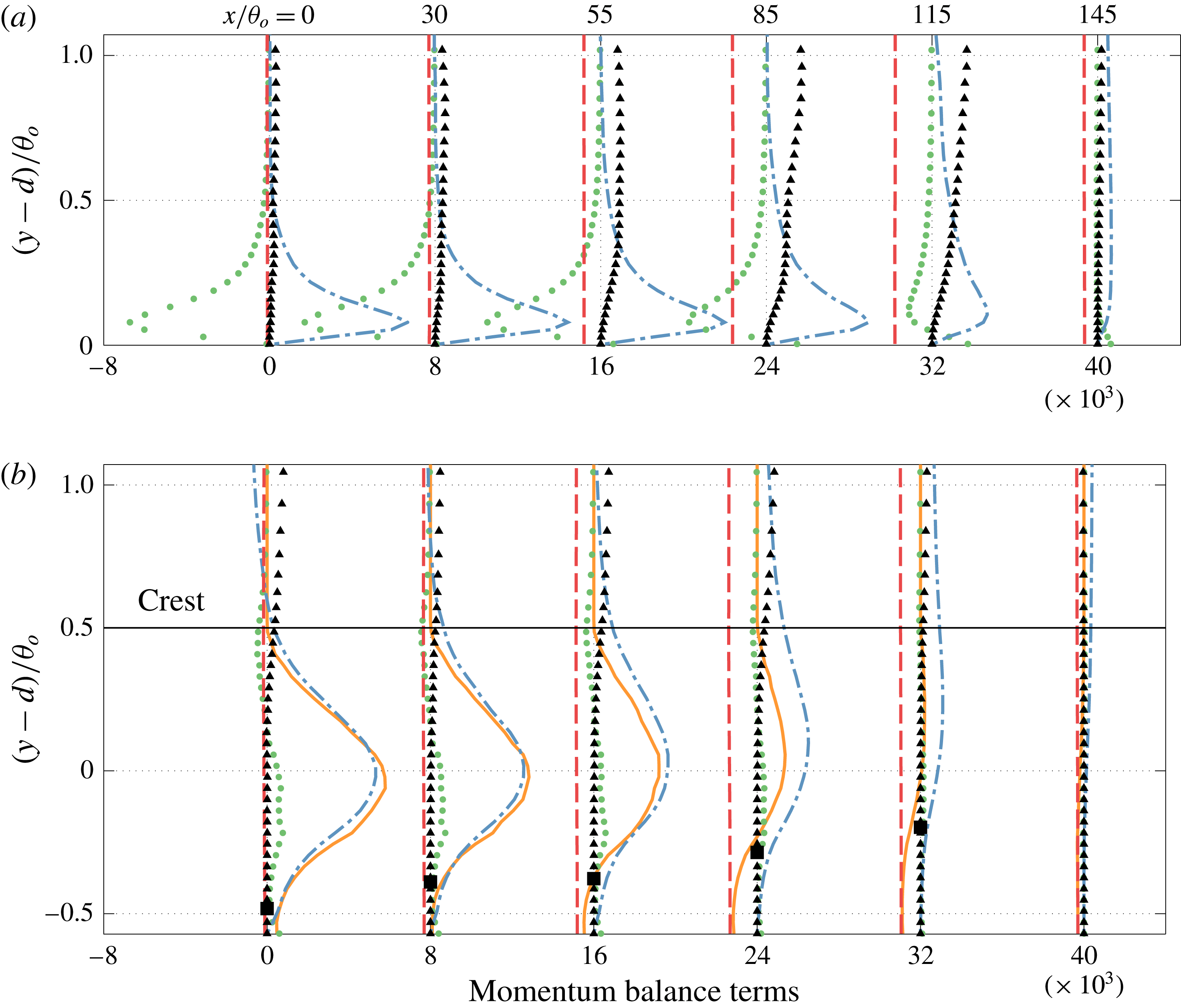
The terms in the smooth-wall case are compared in figure 9(a). In the ZPG region, the Reynolds stress divergence
 ${\mathcal{R}}$
balances the total diffusion
 ${\mathcal{D}}$
. In this region a constant stress layer is present, and the wall stress can be obtained by extrapolating the Reynolds shear stress. In the APG region, the pressure gradient becomes significant and causes the flow to decelerate (the acceleration is the negative of the advection
 ${\mathcal{A}}$
). These two terms nearly balance each other away from the wall (
 $(y-d)/\unicode[STIX]{x1D703}_{o}>0.35$
at
 $x/\unicode[STIX]{x1D703}_{o}=55$
and
 $(y-d)/\unicode[STIX]{x1D703}_{o}>0.7$
at
 $x/\unicode[STIX]{x1D703}_{o}=85$
), as in inviscid flow. In the vicinity of the wall, however, the pressure gradient (and, to a lesser extent, the flow deceleration) alter the balance between diffusion and Reynolds stresses:
 ${\mathcal{D}}$
is now significantly lower than
 ${\mathcal{R}}$
. Also note that the wall stress is equal to the integral of the difference between pressure gradient (which is nearly constant across the boundary layer, as discussed before) and advection term; this difference is significant for
 $y<\unicode[STIX]{x1D703}_{o}$
; above this height the difference is small, but still contributes to the integral, since it extends over a much wider range.
In the rough case, the balance is very different: below the roughness crest (which is located at
 $(y-d)/\unicode[STIX]{x1D703}_{o}=0.5$
) the drag is nearly equal to the Reynolds stress divergence in the ZPG region. The term
 ${\mathcal{F}}_{u}$
is the sum of the viscous drag around the roughness elements, and the form drag due to the pressure (which is generally lower in the wake of the elements). The diffusion term is negligible (due to the low velocity below the crest) as is the advection, which becomes significant only above the crest. Thus, the momentum transfer due to the turbulent fluctuations causes the drag. In the APG region, on the other hand, the pressure gradient enters the balance, and the drag decreases. It should be pointed out that this pressure gradient is the external pressure difference, which is nearly constant in the wall-normal direction as shown. The form drag induced by the roughness is implicitly included in the body force term. We cannot separate form and friction drag with this model; however, because of the low flow velocity and velocity gradients below the crest, we conjecture that the fact that the mean pressure is increasing in the streamwise direction results in a decrease of the form drag. As the increasing pressure causes the drag to decrease, around
 $x/\unicode[STIX]{x1D703}_{o}\simeq 85$
the integral of
 ${\mathcal{F}}_{u}$
(and, hence,
 $C_{f}$
) becomes zero, and negative thereafter. At this location, however, the flow is reversed only in a thin region well below the roughness crest. The region of reversed flow thickens with
 $x$
, and the zero velocity point reaches the crest only at
 $x/\unicode[STIX]{x1D703}_{o}=136$
, where the flow detaches from the wall.
Capturing this flow reversal can be very challenging for experiments because measurements in the roughness layer are difficult. It also raises some issues for the modelling of roughness effects within the framework of turbulence models for the Reynolds-averaged Navier–Stokes equations, which generally bypass the region below the virtual wall, and model the effect of roughness through an increased eddy viscosity, that accounts for the more vigorous turbulent fluctuations. Since these models cannot capture the flow reversal below the crest, their accuracy in the prediction of the drag may be limited (Dutta et al. Reference Dutta, Nicolle, Giroux, Piomelli and Fortes Patella2016, Reference Dutta, Nicolle, Giroux and Piomelli2017).
The increase in the shape factor is an indicator of flow separation, but not ideal for the precise prediction of the separation point. For the smooth-wall case, at the separation point
 $H=3$
, similar to the range reported in previous studies, and the criterion
 $H>2.5$
leads to a slightly early prediction of separation. In the rough-wall case, however, the shape factor is approximately 40 % larger than the smooth case even in the ZPG region, and a value
 $H=2.5$
is attained much before separation, where
 $H=3.6$
.
Contours of velocity fluctuations in a plane parallel to the wall. (a) Smooth wall;
 $y/\unicode[STIX]{x1D703}_{o}=0.04$
; (b) rough wall,
 $(y-d)/\unicode[STIX]{x1D703}_{o}=0.2$
(below the crest); (c) rough wall, roughness crest. The thick line represents the average separation (
 $U=0$
); the contour lines show the roughness elements in the plane of the fluctuations in (b), and immediately below the crest in (c).

Another difference between smooth and rough cases is the fact that, in the latter, the point where the intermittency is
 $\unicode[STIX]{x1D6FE}_{u}=0.5$
does not correspond to flow detachment. This is due to the presence of recirculation regions behind the roughness elements; at the virtual wall, for instance (where 80 % of the area is occupied by fluid) reversed flow occurs approximately 20 % of the time even in the ZPG region. The APG increases this percentage until
 $\unicode[STIX]{x1D6FE}_{u}=0.5$
(at the roughness crest) at
 $x/\unicode[STIX]{x1D703}_{o}\simeq 105$
. At this location although the flow is reversed 50 % of the time, the mean velocity is still greater than zero: the reversed-flow regions, being in the wake of the roughness elements, have very low velocity, while in the areas where the fluid is moving downstream the velocity is much larger, as the flow is channelled in the regions between roughness elements, a phenomenon observed in experimental and numerical studies (Hong, Katz & Schultz Reference Hong, Katz and Schultz2011; Yuan & Piomelli Reference Yuan and Piomelli2014a
). This is illustrated in figure 10. In the rough-wall case, in the separation region where the area occupied by reversed flow is roughly half of the total area (
 $x/\unicode[STIX]{x1D703}_{o}=110-130$
) the flow in the reversed-flow region is generally slower than in the forward-moving ones. Figure 10(b,c) indicates that there is a high correlation between the high-speed regions, and the preferential ‘channels’ between roughness elements. When the wall is smooth, on the other hand, the range of positive and negative velocities is the same (figure 10
a) at the separation point. Also note that large-scale spanwise intermittency, which are footprints of the streamwise structures in the separated shear layer, can be observed in both cases upstream of the average separation, and a short distance after it. In the rough-wall case these footprints extend deep into the roughness layer (figure 10
c). The local distribution of the roughness seems has no effect on these large structures. In some regions with fewer roughness elements, such as the one near
 $x=125$
and
 $z=22$
(figure 10
b,c), the velocity fluctuation is negative, while in some other regions of this type such as the one near
 $x=145$
and
 $z=10$
, the fluctuation is positive. This indicates that the large-scale motions play an important role in the development of backflow events.
4 Turbulence statistics
Contours of the turbulent kinetic energy (TKE),
 ${\mathcal{K}}=\langle u_{i}^{\prime }u_{i}^{\prime }\rangle /2$
, and Reynolds shear stresses,
 $-\langle u^{\prime }v^{\prime }\rangle$
, are shown in figure 11. A high TKE region occurs in the shear layer at the uphill side of the separation bubble before the crest. The maximum TKE level is higher in the rough-wall case, both in the near-wall region and in the separated shear layer. In the smooth-wall case, the Reynolds shear stress is largest near reattachment, due to the impingement of the vortices formed in the shear layer (Na & Moin Reference Na and Moin1998); when the wall is rough, on the other hand, the higher levels of
 $-\langle u^{\prime }v^{\prime }\rangle$
near the wall result in higher stress at the beginning of the shear layer. If scaled by the friction velocity at the reference section (not shown) much of the roughness effect is removed: the TKE in the separated shear layer is much lower in the rough-wall case, while the near-wall peaks are comparable. This indicates that the (i) Townsend’s similarity hypothesis also applies in the APG region, and (ii) the flow in the separated shear layer does not have memory of the higher TKE in the near-wall region, suggesting that local production mechanisms due to the inflectional instability are dominant. Roughness still plays a role in the early development of the shear layer: the growth of the TKE there begins earlier (relative to the separation point) in the rough-wall case and the peak TKE occurs close to the separation point, while in the smooth-wall case it is closer to the top of the recirculation bubble.
Contours of: (a,b) turbulent kinetic energy
 ${\mathcal{K}}/U_{o}^{2}$
; (c,d) Reynolds shear stress
 $-10^{3}\times \langle u^{\prime }v^{\prime }\rangle /U_{o}^{2}$
. ——
 $\unicode[STIX]{x1D6FF}$
; – - –
 $\unicode[STIX]{x1D713}_{o}$
; (a,c) smooth wall; (b,d) rough wall.

To understand these effects, we consider the production of TKE,
 ${\mathcal{P}}_{{\mathcal{K}}}$
, in a frame of reference
 $s-n$
, in which
 $s$
is tangent to the streamline and
 $n$
is perpendicular to it. While the production itself is a scalar, and thus invariant to a rotation of the frame of reference, its individual components are not. Transforming from the (
 $x-y$
) frame to the (
 $s-n$
) one results in additional terms in the velocity gradient tensor (Richmond, Chen & Patel Reference Richmond, Chen and Patel1986; Chen, Patel & Ju Reference Chen, Patel and Ju1990), which, in this case, are negligible. Thus, the production takes a form very similar to that in Cartesian coordinates:
 $$\begin{eqnarray}\displaystyle & \displaystyle {\mathcal{P}}_{{\mathcal{K}}}\simeq \underbrace{-\langle u_{n}^{\prime }u_{n}^{\prime }\rangle \frac{\unicode[STIX]{x2202}U_{n}}{\unicode[STIX]{x2202}n}-\langle u_{s}^{\prime }u_{s}^{\prime }\rangle \frac{\unicode[STIX]{x2202}U_{s}}{\unicode[STIX]{x2202}s}}_{{\mathcal{P}}_{{\mathcal{K}}}^{\unicode[STIX]{x1D70E}}}\underbrace{-\langle u_{s}^{\prime }u_{n}^{\prime }\rangle \frac{\unicode[STIX]{x2202}U_{s}}{\unicode[STIX]{x2202}n}}_{{\mathcal{P}}_{{\mathcal{K}}}^{\unicode[STIX]{x1D70F}}} & \displaystyle\end{eqnarray}$$
in which
 ${\mathcal{P}}_{{\mathcal{K}}}^{\unicode[STIX]{x1D70E}}$
and
 ${\mathcal{P}}_{{\mathcal{K}}}^{\unicode[STIX]{x1D70F}}$
denote the normal stress and shear stress contributions to the production, respectively.
Figure 12 shows the contours of these quantities. In both cases, the normal component is much smaller than the shear one; it is significant only near the separation point, where the streamline curvature is significant, and near reattachment, because of the impinging vortices. Intense TKE is generated by the shear production in the vicinity of the surface before flow detachment. While in the smooth-wall case there are two somewhat distinct regions of high production, one near the wall, the other in the separated shear layer, in the rough-wall case they are combined: the thicker layer of strong TKE in the attached region means that high
 $\langle u^{\prime }v^{\prime }\rangle$
starts contributing to the shear production earlier; thus, the peak TKE occurs much closer to the separation point in the rough-wall case.
Contours of (a,b) normal production of TKE,
 ${\mathcal{P}}_{{\mathcal{K}}}^{\unicode[STIX]{x1D70E}}$
; (c,d) shear production of TKE,
 ${\mathcal{P}}_{{\mathcal{K}}}^{\unicode[STIX]{x1D70F}}$
, normalized by
 $10^{-5}\times U_{o}^{3}/\unicode[STIX]{x1D703}_{o}$
. ——
 $\unicode[STIX]{x1D6FF}$
; – - –
 $\unicode[STIX]{x1D713}_{o}$
; - - - streamline passing through
 $(y-d)/\unicode[STIX]{x1D703}_{o}=2.5$
at
 $x=0$
. (a,c) smooth wall; (b,d) rough wall.

The productions of the normal and shear stresses in the
 $s-n$
frame are:
 $$\begin{eqnarray}\displaystyle & \displaystyle {\mathcal{P}}_{ss}\simeq -2\langle u_{s}^{\prime }u_{s}^{\prime }\rangle \frac{\unicode[STIX]{x2202}U_{s}}{\unicode[STIX]{x2202}s}-2\langle u_{s}^{\prime }u_{n}^{\prime }\rangle \frac{\unicode[STIX]{x2202}U_{s}}{\unicode[STIX]{x2202}n}=-2\langle u_{s}^{\prime }u_{s}^{\prime }\rangle \frac{\unicode[STIX]{x2202}U_{s}}{\unicode[STIX]{x2202}s}+2{\mathcal{P}}_{{\mathcal{K}}}^{\unicode[STIX]{x1D70F}}\simeq 2{\mathcal{P}}_{{\mathcal{K}}}^{\unicode[STIX]{x1D70F}} & \displaystyle\end{eqnarray}$$
 $$\begin{eqnarray}\displaystyle & \displaystyle {\mathcal{P}}_{nn}\simeq -2\langle u_{n}^{\prime }u_{n}^{\prime }\rangle \frac{\unicode[STIX]{x2202}U_{n}}{\unicode[STIX]{x2202}n}\simeq 0 & \displaystyle\end{eqnarray}$$
 $$\begin{eqnarray}\displaystyle & \displaystyle {\mathcal{P}}_{sn}\simeq -\langle u_{n}^{\prime }u_{n}^{\prime }\rangle \frac{\unicode[STIX]{x2202}U_{s}}{\unicode[STIX]{x2202}n} & \displaystyle\end{eqnarray}$$
(additional terms in curvilinear coordinates are negligible). The TKE production terms, mean shear and Reynolds stresses in the
 $s-n$
coordinates are examined along a streamline passing through the high TKE and shear production region after flow separation (showed in figure 12), to identify the critical processes affecting the TKE. Their profiles are plotted in figure 13. Other streamlines shows similar trends.
Profiles of quantities along the streamline passing through the high TKE region in the separated shear layer. (a) Reynolds stresses, normalized by
 $U_{o}^{2}$
; ▿
 $\langle u_{s}^{\prime }u_{s}^{\prime }\rangle$
; ▫ (red)
 $\langle u_{s}^{\prime }u_{n}^{\prime }\rangle$
; ○ (blue)
 $\langle u_{n}^{\prime }u_{n}^{\prime }\rangle$
. (b) Velocity gradients, normalized by
 $U_{o}/\unicode[STIX]{x1D703}_{o}$
. ▫ (red)
 $\unicode[STIX]{x2202}U_{s}/\unicode[STIX]{x2202}n$
; ○ (blue)
 $10\times \unicode[STIX]{x2202}U_{s}/\unicode[STIX]{x2202}s$
. (c) Normal and shear production of TKE, normalized by
 $U_{o}^{3}/\unicode[STIX]{x1D703}_{o}$
. ▫ (red) Shear production
 $P_{{\mathcal{K}}}^{\unicode[STIX]{x1D70F}}$
; ○ (blue) normal production
 $P_{{\mathcal{K}}}^{\unicode[STIX]{x1D70E}}$
. The thin vertical lines without markers represent the average separation and reattachment (
 $U=0$
). —— Smooth wall, - - - rough wall.

In the FPG region, for
 $0<x/\unicode[STIX]{x1D703}_{o}<50$
, the only significant velocity gradient is
 $\unicode[STIX]{x2202}U_{s}/\unicode[STIX]{x2202}n$
, which is much higher in the rough-wall case (see also figure 7(c)). The Reynolds stresses are also higher, resulting in much larger production of
 $\langle u_{s}^{\prime }u_{n}^{\prime }\rangle$
(which is equal to
 $\langle u^{\prime }v^{\prime }\rangle$
in this region of attached flow) and
 $\langle u_{s}^{\prime }u_{s}^{\prime }\rangle$
(equal to
 $\langle u^{\prime }u^{\prime }\rangle$
). These two stress components become, therefore, increasingly larger (in magnitude) than in the smooth case.
 $\langle u_{n}^{\prime }u_{n}^{\prime }\rangle$
is small, and so is its production; this stress component, therefore, receives energy through the pressure redistribution term, as in canonical boundary layers.
For
 $x/\unicode[STIX]{x1D703}_{o}>50$
the APG becomes important, and the flow begins to slow down (
 $\unicode[STIX]{x2202}U_{s}/\unicode[STIX]{x2202}s$
is scaled up by a factor of 10 in figure 13(b);
 $\unicode[STIX]{x2202}U_{n}/\unicode[STIX]{x2202}s$
is zero and
 $\unicode[STIX]{x2202}U_{n}/\unicode[STIX]{x2202}n$
is small). This causes an increase of the normal production of TKE and the production of
 $\langle u_{s}^{\prime }u_{s}^{\prime }\rangle$
(i.e.
 $\langle u^{\prime }u^{\prime }\rangle$
). The shear stress magnitude starts to increase in the outer layer. This process continues as the APG becomes stronger. The peak of
 $P_{{\mathcal{K}}}^{\unicode[STIX]{x1D70F}}$
occurs very near the separation point in both cases. After flow detachment the separated shear layer becomes similar to a mixing layer, the mean shear reduces rapidly and leads to the reduction of Reynolds stresses and TKE.
There are several differences in the TKE generation mechanisms between the smooth and rough cases. First, the strong shear production of TKE in the rough-wall cases due the momentum deficit in the ZPG region is maintained at a near-constant high level due to the amplified Reynolds stresses (i.e. more active turbulence) that balance the decrease of
 $\unicode[STIX]{x2202}U_{s}/\unicode[STIX]{x2202}n$
in the streamwise direction; in the smooth-wall case, on the contrary, the low velocity gradient cannot trigger shear production away from the wall. Second, on the smooth wall both normal Reynolds stresses and velocity gradient remain nearly constant well into the APG region (
 $x/\unicode[STIX]{x1D703}_{o}\simeq 100$
) until flow deceleration promotes the turbulence; in the rough-wall case, on the other hand, the Reynolds stresses begin to increase earlier, and the constant production results in higher TKE. Thus, it seems that the difference in TKE production between the smooth and rough cases is not due to a local behaviour; the flow history plays an important role.
The mean velocity, TKE and Reynolds shear stress (RSS) profiles normal to the streamline passing through
 $(y-d)/\unicode[STIX]{x1D703}_{o}$
in the uphill side of the separated boundary layer are plotted in figure 14. The location examined is chosen so that the TBL has just detached from the surface: the streamline reaches
 $(y-d)/\unicode[STIX]{x1D703}_{o}=5$
for the plots showed. Thus unlike comparing the quantities in the same streamwise location in figure 13, here we make the comparison at similar location relative to the separation point. The quantities are transformed to the streamline coordinates (origin and coordinates are showed in figure 14
a,b), which leads to the positive
 $U_{s}$
and RSS in the backflow region (
 $d_{n}/\unicode[STIX]{x1D703}_{o}<-2$
region in figure 14
c,d). Note that after the streamline separates from the
 $U=0$
location,
 $U_{s}$
increases along it so the backflow region appears at negative
 $n$
-coordinates instead of at the origin. It can be seen that the higher velocity gradient and amplified TKE in the rough-wall case appear not only when the two cases are compared at same
 $x$
-locations as in figure 13, but also when the comparison is made at corresponding locations relative to the separation point in each case. Given that the shear stress are similar between the two cases at this region (figure 14
d), higher velocity gradient due to roughness (figure 14
c) leads to larger shear production at the beginning of the separation. This results, together with figure 13, explain how the TKE peaks earlier and is more intense throughout the separated shear layer in the rough-wall cases: the cause is the higher mean velocity gradient due to momentum deficit; the earlier occurrence of peak is mainly due to the prompt shear production even though the RSS near the separation point are similar. The differences during this early stage of the separated shear layer development lead to further discrepancy downstream.
Statistics normal to the separated streamline in the uphill side of the separation bubble. The locations considered and streamline coordinates are shown in (a,b) (for line style refer to figure 12. Dotted line represents the line in the
 $n$
-direction that the profiles are examined along). (a) Smooth wall; (b) rough wall; (c),
 $U_{s}$
. (d) Lines, TKE; lines with marker,
 $\langle u_{s}^{\prime }u_{n}^{\prime }\rangle$
. —— smooth wall, - - - rough wall in (c,d).

In figure 13, both production terms of the TKE are attenuated near the top of the separation bubble. Examining several other streamlines further away in the upper part of the separated shear layer (not shown), negative
 $P_{{\mathcal{K}}}^{\unicode[STIX]{x1D70F}}$
and
 $P_{{\mathcal{K}}}^{\unicode[STIX]{x1D70E}}$
are observed near the separation bubble crest (
 $x/\unicode[STIX]{x1D703}_{o}=205$
). Their peak values are one order of magnitude smaller than the positive peak on the uphill side. This result agrees with previous studies (Na & Moin Reference Na and Moin1998; Spalart & Coleman Reference Spalart and Coleman1997; Skote & Henningson Reference Skote and Henningson2002; Abe et al.
Reference Abe, Mizobuchi, Matsuo and Spalart2012). The negative shear stress production is weaker in the rough-wall case: the higher
 $\unicode[STIX]{x2202}U_{s}/\unicode[STIX]{x2202}n$
extending up to the bubble crest mitigates the decrease of the shear stress (refer to (4.4)).
5 Conclusions
We have examined the combined effects of roughness and adverse pressure gradient (APG) on turbulent boundary layers with separation. The aim of this study was to investigate the characteristics of the separation and the difference in the dynamics of flow separation between the rough and smooth cases. To perform such investigation we have carried out large-eddy simulations of a flat-plate turbulent boundary layer subjected to an adverse-to-favourable pressure gradient. The flow forms a closed separation bubble due to the large pressure gradient induced by the suction–blowing velocity distribution prescribed at the top boundary of the calculation domain. Virtual sand grain roughness on the surface is modelled by an immersed boundary method. An average roughness height equal to 7 % of the boundary layer thickness in the zero-pressure-gradient (ZPG) region was chosen to remain in the fully rough regime, while not significantly blocking the boundary layer.
Streamline detachment occurs earlier and the separation region is substantially larger for the rough-wall case. This is due to the momentum deficit caused by the roughness. In the smooth-wall case various criteria (including
 $C_{f}=0$
and backflow intermittence
 $\unicode[STIX]{x1D6FE}=0.5$
) predict separation reasonably close to the position of detachment of the mean streamline. In the rough-wall case, however, these three criteria do not coincide.
 $C_{f}=0$
occurs much earlier than the flow detachment: in the APG region, the adverse pressure gradient plays an important role, decreasing the drag (presumably, the form drag) and causing it to go to zero while the flow, at least over the roughness crest, is still attached. Flow reversal is observed in a layer below the crest; this layer becomes thicker and eventually emerges from the roughness sublayer, causing the flow detachment. The presence of recirculation regions behind roughness elements changes the intermittency of the near-wall turbulence. The fluid moves very slowly in the wake of the roughness elements, while it is channelled between elements with much larger velocity. The footprint of the flow between the roughness element can still be detected above the roughness crest. Thus, the flow can be reversed at 50 % of the points, but its mean velocity is still positive, and no detachment occurs.
The separated shear layer exhibits higher turbulent kinetic energy (TKE) in the rough-wall case, both in the near-wall region and in the separated shear layer. Townsend’s similarity hypothesis still holds for the near-wall peak stresses. In the separated shear layer, roughness leads to an early growth of TKE and the peak TKE occurs close to the separation point. The local production mechanism due to the inflectional instability in such region is affected by the roughness indirectly: in the ZPG region, the significantly higher wall-normal velocity gradient in the rough-wall case resulting in a much larger production of the Reynolds stresses. These amplified Reynolds stresses, representing more active turbulence, help to maintain a near-constant production of TKE in the APG region. Such process does not occur in the smooth-wall case because of the lack of significant mean velocity gradient in the outer layer, which acts as the original trigger of the shear stress TKE production and the Reynolds stresses’ production. Even though the high TKE region seems to have no memory of the near-wall amplified turbulence by roughness, it is still changed by the roughness due to its momentum deficit effect. In particular, the process by which the mean velocity gradient affects the TKE in the separated shear layer is non-local: flow history plays an important role. Meanwhile, the attenuation of the TKE production near the top of the separation bubble has been found to be due both to the normal and shear stress production. The rough-wall case shows less reduced production, since the mean shear mitigates the decrease of the shear stress.
Future studies should examine the roughness effects with different flow histories, in particular, various APG applied at the free stream. In the current study the APG is increased gradually, while in realistic flow it can be more abrupt, leading to significant deceleration of the flow, as well as much higher normal stress production. The high velocity gradient caused by the roughness may not have the chance to cause significant difference in the shear stress production in such situation. Many recent studies on flow separation are concerned with the effects of flow history. In the current study the pressure gradients experienced by the TBL in the two cases are slightly different near the separation point (refer to figure 4). It would be valuable to examine the response of the TBL under the same APG history. It would also be desirable to extend the range of simulation parameters. For example, a large-scale separation
 $\unicode[STIX]{x1D6FF}/k$
and higher Reynolds numbers. As usual, this is hampered by the computational resources required: the current rough-wall case, for instance, requires 260 thousand CPU hours on a 128-node, 2.5 GHz Intel cluster. A Reynolds number higher by a factor of two would require approximately 2 million CPU hours, which is presently not feasible.
Acknowledgements
The authors acknowledge the support from Hydro-Québec and the Natural Science and Engineering Research Council of Canada (NSERC) under the Collaborative Research and Development program (grant no. CRDPJ 418786-11). The simulations were performed at the Center for Advanced Computing, Queen’s site. U.P. also acknowledges the support of the Canada Research Chair program.
Appendix A. Immersed boundary method
In this study, the immersed boundary method (IBM) with volume-of-fluid (VOF) approach is employed to represent the roughness geometry, while maintaining the simplicity of the Cartesian solver. This technique was first applied by Scotti (Reference Scotti2006) to the study of roughness with DNS. In particular, the interface of the roughness does not change in time, nor with the flow. Thus the volume fraction of the fluid,
 $\unicode[STIX]{x1D719}$
, in each grid cell is calculated in pre-processing. For details on the implementation of this method in the flow solver the readers are referred to Scotti (Reference Scotti2006) and Yuan & Piomelli (Reference Yuan and Piomelli2014a
).
Iso-surfaces of (a)
 $\unicode[STIX]{x1D719}=0.5$
; (b) time-averaged streamwise velocity equals zero, near the start of the roughness patch. Coloured by distance from the bottom boundary.

Note that information regarding the interface shape, such as intersections with the grid cells and surface normal, are not described in this approach. Although the roughness geometry is not perfectly resolved unless very fine grids are used around the elements, it has been shown that this approach is sufficient for the study of roughness in boundary layers over rough surfaces (Scotti Reference Scotti2006; Yuan & Piomelli Reference Yuan and Piomelli2014a ) since the description of the rough surface is only an approximation to real sand paper. Representing this virtual sand paper by the current grid resolution preserves the general geometry of the surface made of randomly oriented ellipsoids (see figure 15) and the drag it introduced (refer to figure 7 which shows that the momentum deficit caused by the roughness satisfies well the logarithmic relation). Further refining the grid or using other numerical methods to better resolve the flow around the actual ellipsoid element may provide more detailed flow fields within the roughness layer, but it is not expected to change the overall results (Yuan & Piomelli Reference Yuan and Piomelli2014a ).
The virtual origin,
 $d$
, is calculated as the vertical distance to the centroid of the moment of the mean body force (Yuan & Piomelli Reference Yuan and Piomelli2014a
)
 $$\begin{eqnarray}\displaystyle & \displaystyle d=\int _{0}^{y_{c}}y\langle f_{i}(y)\rangle \,\text{d}y\bigg/\int _{0}^{y_{c}}\langle f_{i}(y)\rangle \,\text{d}y. & \displaystyle\end{eqnarray}$$
The virtual sand grain model gives
 $d\approx 0.8k$
for the attached TBL, and is insensitive to the pressure gradient (Yuan & Piomelli Reference Yuan and Piomelli2014a
). The reason to use
 $d$
as the displacement rather than others is that this choice agrees with the scenario of flow over smooth wall, in which the origin is at the wall where the shear stress is applied. Moreover, it is important to emphasize that term ‘displacement’ or ‘shifting’ of the velocity profile inherently indicates the existence of certain kind of flow similarity in the mean flow in the vicinity of the roughness layer, i.e. the logarithmic behaviour of velocity profile in wall units. In the near-wall region, the flow depends primarily on the total drag (so the friction velocity is the characteristic velocity scale) but only weakly on any other property of the flow. Similarly, the flow in such a region cannot distinguish any details of the drag distribution due to roughness geometry except the level at which this stress appears to act (Jackson Reference Jackson1981).



