1 Introduction
Oscillatory time-periodic flows arise in many engineering and environmental processes. In near-shore seas, waves propagating over a slope may be skewed. The degree of skewness is dependent on the wave shape (period, height and depth) and plays a significant role in coastal hydrodynamics. Velocity skewness generates a wave with a narrow sharp crest and a broad flat trough, while acceleration skewness establishes a wave asymmetry. Voluminous numerical and experimental investigations have modelled the effects of skewness on boundary layer flows and net sediment transport (only a few are cited below). Ribberink & Al-Salem (Reference Ribberink and Al-Salem1995), Dibajnia & Watanabe (Reference Dibajnia and Watanabe1998) and O’Donoghue & Wright (Reference O’Donoghue and Wright2004) considered the effects brought about by velocity skewness, while the effects of acceleration skewness on the motion of oscillatory flows have been studied by, among others, Madsen (Reference Madsen and O’Brien1974), Drake & Calantoni (Reference Drake and Calantoni2001) and Nielsen & Callaghan (Reference Nielsen and Callaghan2003). Experiments undertaken by Watanabe & Sato (Reference Watanabe, Sato and Smith2004) have shown that net sand transport is non-zero in an acceleration-skewed oscillatory flow and is always convected in the direction of highest acceleration. Furthermore, net transport is enhanced by increasing the level of acceleration skewness. These observations were later confirmed experimentally by Abreu et al. (Reference Abreu, Silva, Sancho and Temperville2010) using an oscillating flow tunnel.
Previous studies on the hydrodynamic stability of acceleration-skewed flows have focussed on turbulent flow characteristics. van der A et al. (Reference van der A, O’Donoghue, Davies and Ribberink2011) undertook an experimental study of acceleration-skewed boundary layers over a rough wall and showed that the turbulence intensities were enhanced by increasing the degree of acceleration skewness. Direct numerical simulations were carried out by Scandura, Faraci & Foti (Reference Scandura, Faraci and Foti2016) for acceleration-skewed flows over a smooth wall. Turbulent near-wall streaky structures were observed for several acceleration-skew settings and flow conditions based on a Reynolds number  $Re\in [300,700]$. (A formal definition for the Reynolds number is given below in (2.4), while it is noted that Scandura et al. (Reference Scandura, Faraci and Foti2016) defined the Reynolds number as
 $R_{\unicode[STIX]{x1D6FF}}=2Re$ in their numerical investigation.)
This paper is concerned with the linear stability of acceleration-skewed oscillating flows. Asymmetric motion can be quantified by the wave acceleration about the crest and trough. Drake & Calantoni (Reference Drake and Calantoni2001) modelled the effects of wave shape on bed load transport. In their study the velocity profile  $u$ was proportional to
 $$\begin{eqnarray}u(t)\propto \mathop{\sum }_{n=0}^{4}\frac{1}{2^{n}}\sin ([n+1]\unicode[STIX]{x1D714}t+n\unicode[STIX]{x1D719}),\end{eqnarray}$$
for an integer  $n$, a frequency
 $\unicode[STIX]{x1D714}$ and a waveform parameter
 $\unicode[STIX]{x1D719}$. Acceleration skewness was established for
 $\unicode[STIX]{x1D719}=0$; a sawtooth shaped wave develops that is a characteristic of waves breaking in the surf zone. A velocity-skewed waveform is realised for
 $\unicode[STIX]{x1D719}=\unicode[STIX]{x03C0}/2$. Drake and Calantoni’s model was later generalised by Abreu et al. (Reference Abreu, Silva, Sancho and Temperville2010) as
 $$\begin{eqnarray}u(t)\propto \mathop{\sum }_{n=0}^{\infty }\frac{1}{\unicode[STIX]{x1D709}^{n}}\sin ([n+1]\unicode[STIX]{x1D714}t+n\unicode[STIX]{x1D719}),\end{eqnarray}$$
where the parameter  $\unicode[STIX]{x1D709}$ represents the degree of wave skewness.
van der A et al. (Reference van der A, O’Donoghue, Davies and Ribberink2011) implemented an alternative formula for modelling asymmetric wave motion in an oscillating flow tunnel,
 $$\begin{eqnarray}u(t)\propto \mathop{\sum }_{n=1}^{N}\frac{(2\unicode[STIX]{x1D6FD}-1)^{n-1}}{n}\sin (n\unicode[STIX]{x1D714}t),\end{eqnarray}$$
for an integer  $N$. The degree of acceleration skewness was characterised by the parameter
 $\unicode[STIX]{x1D6FD}$ (that is described in § 2). More recently, Scandura et al. (Reference Scandura, Faraci and Foti2016) utilised the van der A et al. (Reference van der A, O’Donoghue, Davies and Ribberink2011) model in their numerical study.
For sufficiently large levels of acceleration skewness the wave acquires a sawtooth shape. However, when the wave acceleration about the crest matches that about the trough the oscillatory motion is symmetric and a Stokes layer forms. The Stokes layer is the archetypical model for investigating unsteady fluid flow phenomena. An early literature review on time-periodic flows was given by Davis (Reference Davis1976), while Von Kerczek & Davis (Reference Von Kerczek and Davis1974) and Hall (Reference Hall1978) undertook linear stability investigations on the respective finite and semi-infinite Stokes layer models. Linear stability calculations were based on Floquet theory that assumes infinitesimal perturbations to the time-periodic base flow are decomposed into the form  $\exp (\unicode[STIX]{x1D707}t)f$. Here
 $f$ is a
 $2\unicode[STIX]{x03C0}$-periodic function in time, while the net growth or decay of the disturbance is characterised by the real part of the Floquet exponent
 $\unicode[STIX]{x1D707}$.
Hall (Reference Hall1978) was unable to locate any linearly unstable disturbances for a Reynolds number  $Re<160$, while Von Kerczek & Davis (Reference Von Kerczek and Davis1974) were unable to detect any linear instabilities up to
 $Re=400$. It was only much later, following the advancement of computational technology, that Blennerhassett & Bassom (Reference Blennerhassett and Bassom2002) were able to trace part of the neutral stability curve and determine the critical conditions for the onset of linear instability;
 $Re_{c}\sim 707.84$. This was later confirmed separately by Luo & Wu (Reference Luo and Wu2010) and Thomas et al. (Reference Thomas, Bassom, Blennerhassett and Davies2010).
In the subsequent study Floquet theory is applied to the family of flows generated by an acceleration-skewed oscillating planar wall. Acceleration skewness is achieved using the formula implemented by van der A et al. (Reference van der A, O’Donoghue, Davies and Ribberink2011). This particular model was chosen over the alternative methods (Drake & Calantoni Reference Drake and Calantoni2001; Abreu et al. Reference Abreu, Silva, Sancho and Temperville2010) as it establishes smoother waveforms for large levels of acceleration skewness. Linear stability analysis is then performed using a two-dimensional vorticity form of the linearised Navier–Stokes equations that is based on the formulation developed by Davies & Carpenter (Reference Davies and Carpenter2001). This particular method was chosen over alternative approaches to illustrate the robustness of the numerical scheme. Additionally, the method provides further confirmation of the earlier results by Blennerhassett & Bassom (Reference Blennerhassett and Bassom2002, Reference Blennerhassett and Bassom2006) on the symmetrically oscillating Stokes layer who employed a vorticity-streamfunction formulation coupled with a pseudospectral technique (Fornberg Reference Fornberg1996; Trefethen Reference Trefethen2000).
The remainder of this paper is outlined as follows. In the subsequent section the acceleration-skewed oscillating wall motion is modelled and the perturbation equations are described in § 3. Critical conditions for linear instability and the structure of the eigenfunctions are presented in § 4 for variable acceleration-skewed flow settings. Finally, conclusions are given in § 5.
2 Base flow
Consider the two-dimensional flow that develops in a semi-infinite layer of viscous incompressible fluid that is bounded by a flat plate located in the plane  $y=0$. The wall oscillates back and forth along the
 $x$-direction with an acceleration-skewed velocity (van der A et al. Reference van der A, O’Donoghue, Davies and Ribberink2011; Scandura et al. Reference Scandura, Faraci and Foti2016)
 $$\begin{eqnarray}U_{0}=U_{0,max}\mathop{\sum }_{n=1}^{N}\unicode[STIX]{x1D6FE}_{n}\sin (n\unicode[STIX]{x1D714}t),\end{eqnarray}$$
for
 $$\begin{eqnarray}\unicode[STIX]{x1D6FE}_{n}=\frac{\unicode[STIX]{x1D6FC}(2\unicode[STIX]{x1D6FD}-1)^{n-1}}{n},\end{eqnarray}$$
that forces the adjacent body of fluid into an asymmetric sinusoidal motion. Here  $U_{0,max}$ is the maximum wall velocity,
 $N$ is the total number of harmonics used to represent the wall motion,
 $\unicode[STIX]{x1D714}$ is the frequency of oscillation and the coefficient
 $\unicode[STIX]{x1D6FC}$ ensures that
 $\max (U_{0})=U_{0,max}$. Acceleration skewness is quantified by the parameter
 $$\begin{eqnarray}\unicode[STIX]{x1D6FD}=\frac{\dot{U}_{0,max}}{\dot{U}_{0,max}-\dot{U}_{0,min}}~\in [0,1],\end{eqnarray}$$
where  $\dot{U}_{0}$ represents the acceleration of the wall motion (2.1a). The symmetric Stokes layer is realised for
 $\unicode[STIX]{x1D6FD}=0.5$. Furthermore, the Stokes layer is established for any
 $\unicode[STIX]{x1D6FD}$ when
 $N=1$. For
 $\unicode[STIX]{x1D6FD}\neq 0.5$, the number of harmonics
 $N$ must be increased to a sufficient threshold value to achieve the desired asymmetric wall motion.
Oscillatory motion representative of coastal regions is typically realised for  $0.43\leqslant \unicode[STIX]{x1D6FD}\leqslant 0.85$ (Elfrink, Hanes & Ruussink Reference Elfrink, Hanes and Ruussink2006; van der A et al. Reference van der A, O’Donoghue, Davies and Ribberink2011), while at the lower and upper limits for
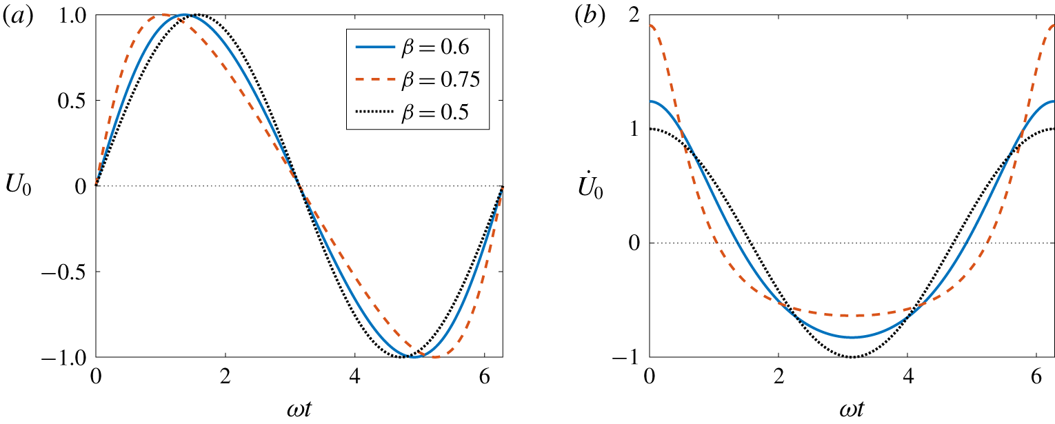
 $\unicode[STIX]{x1D6FD}$ the wall motion is characterised by an oscillating sawtooth function. Figure 1 illustrates the wall velocity
 $U_{0}$ and corresponding wall acceleration
 $\dot{U}_{0}$ as a function of time for
 $\unicode[STIX]{x1D6FD}=0.6$ and 0.75 (based on
 $N=100$). The sinusoidal solution matching to the Stokes layer is included for comparison (dotted line).
(a) Wall velocity  $U_{0}$ and (b) wall acceleration
 $\dot{U}_{0}$ as a function of time
 $\unicode[STIX]{x1D70F}=\unicode[STIX]{x1D714}t$ for variable
 $\unicode[STIX]{x1D6FD}$.

A dimensionless basic state is obtained by setting time  $\unicode[STIX]{x1D70F}=\unicode[STIX]{x1D714}t$, while units of velocity and length are scaled on
 $U_{0,max}$ and the Stokes layer thickness
 $\sqrt{2\unicode[STIX]{x1D708}/\unicode[STIX]{x1D714}}$, respectively. (Here
 $\unicode[STIX]{x1D708}$ is the kinematic viscosity of the fluid.) Given the above scalings, the non-dimensional base flow is defined as
 $$\begin{eqnarray}\boldsymbol{U}_{B}=(U_{B}(y,\unicode[STIX]{x1D70F};\unicode[STIX]{x1D6FD},N),0),\end{eqnarray}$$
where
 $$\begin{eqnarray}U_{B}(y,\unicode[STIX]{x1D70F};\unicode[STIX]{x1D6FD},N)=\mathop{\sum }_{n=1}^{N}\unicode[STIX]{x1D6FE}_{n}\text{e}^{-\sqrt{n}y}\sin (n\unicode[STIX]{x1D70F}-\sqrt{n}y).\end{eqnarray}$$
Additionally, the Reynolds number of the flow
 $$\begin{eqnarray}Re=\frac{U_{0,max}}{\sqrt{2\unicode[STIX]{x1D708}\unicode[STIX]{x1D714}}},\end{eqnarray}$$
which matches the definition used in the earlier study on the symmetric Stokes layer (Blennerhassett & Bassom Reference Blennerhassett and Bassom2002).
3 Perturbation equations
3.1 Formulation
Total velocity and vorticity fields are decomposed as
 $$\begin{eqnarray}(U,V)=(U_{B},0)+\bigg(\frac{\unicode[STIX]{x2202}\unicode[STIX]{x1D713}}{\unicode[STIX]{x2202}y},-\frac{\unicode[STIX]{x2202}\unicode[STIX]{x1D713}}{\unicode[STIX]{x2202}x}\bigg)\quad \text{and}\quad \unicode[STIX]{x1D6FA}=\unicode[STIX]{x1D6FA}_{B}+\unicode[STIX]{x1D714},\end{eqnarray}$$
where the undisturbed vorticity field  $\unicode[STIX]{x1D6FA}_{B}=U_{B}^{\prime }$ and a prime denotes differentiation with respect to the wall-normal direction
 $y$. Perturbation fields
 $\unicode[STIX]{x1D714}$ and
 $\unicode[STIX]{x1D713}$ denote the respective vorticity and streamfunction of a two-dimensional disturbance. As Squires theorem has been extended to unsteady flows (Conrad & Criminale Reference Conrad and Criminale1965; Von Kerczek & Davis Reference Von Kerczek and Davis1974) it is sufficient to restrict the subsequent analysis to two-dimensional perturbations.
Critical conditions for linear instability are determined using a two-dimensional form of the vorticity formulation developed by Davies & Carpenter (Reference Davies and Carpenter2001). The system of governing equations for the perturbations comprises the vorticity transport equation and the wall-normal component of the Poisson equation
 $$\begin{eqnarray}\frac{1}{Re}\frac{\unicode[STIX]{x2202}\unicode[STIX]{x1D714}}{\unicode[STIX]{x2202}\unicode[STIX]{x1D70F}}+U_{B}\frac{\unicode[STIX]{x2202}\unicode[STIX]{x1D714}}{\unicode[STIX]{x2202}x}-U_{B}^{\prime \prime }\frac{\unicode[STIX]{x2202}\unicode[STIX]{x1D713}}{\unicode[STIX]{x2202}x}=\frac{1}{2Re}\unicode[STIX]{x1D6FB}^{2}\unicode[STIX]{x1D714},\end{eqnarray}$$
 $$\begin{eqnarray}\unicode[STIX]{x1D6FB}^{2}\unicode[STIX]{x1D713}=\unicode[STIX]{x1D714},\end{eqnarray}$$
for
 $$\begin{eqnarray}\unicode[STIX]{x1D6FB}^{2}=\frac{\unicode[STIX]{x2202}^{2}}{\unicode[STIX]{x2202}x^{2}}+\frac{\unicode[STIX]{x2202}^{2}}{\unicode[STIX]{x2202}y^{2}}.\end{eqnarray}$$
Boundary conditions at the wall are given as
 $$\begin{eqnarray}\unicode[STIX]{x1D713}=\frac{\unicode[STIX]{x2202}\unicode[STIX]{x1D713}}{\unicode[STIX]{x2202}y}=0\quad \text{on}\quad y=0\end{eqnarray}$$
and on integrating (3.2b) we obtain the following integral constraint for  $\unicode[STIX]{x1D714}$:
 $$\begin{eqnarray}\int _{0}^{\infty }\left(\unicode[STIX]{x1D714}-\frac{\unicode[STIX]{x2202}^{2}\unicode[STIX]{x1D713}}{\unicode[STIX]{x2202}x^{2}}\right)\,\text{d}y=0.\end{eqnarray}$$
Finally, all perturbations are assumed to asymptote towards zero as  $y$ approaches infinity.
3.2 Floquet theory
Primary perturbation fields  $q=\{\unicode[STIX]{x1D714},\unicode[STIX]{x1D713}\}$ (that are given as solutions to (3.2)) are written in exponential form
 $$\begin{eqnarray}q(x,y,\unicode[STIX]{x1D70F})=\hat{q}(y,\unicode[STIX]{x1D70F})\exp \{\unicode[STIX]{x1D707}\unicode[STIX]{x1D70F}+\text{i}ax\}+\text{c.c.}\end{eqnarray}$$
where the wavenumber  $a\in \mathbb{R}$, the Floquet exponent
 $\unicode[STIX]{x1D707}\in \mathbb{C}$,
 $\text{c.c.}$ denotes the complex conjugate and
 $\hat{q}(y,\unicode[STIX]{x1D70F})$ is a
 $2\unicode[STIX]{x03C0}$-periodic function in time. The real part of the Floquet exponent
 $\unicode[STIX]{x1D707}$ specifies the exponential growth or decay rate of the perturbation. As a consequence of the flow symmetry in the Stokes layer, Blennerhassett & Bassom (Reference Blennerhassett and Bassom2002) were able to restrict the imaginary part of
 $\unicode[STIX]{x1D707}$ in their earlier study to the interval
 $0\leqslant \unicode[STIX]{x1D707}_{i}\leqslant 0.5$; Floquet modes occur as a complex conjugate pair
 $\unicode[STIX]{x1D707}_{r}\pm \text{i}\unicode[STIX]{x1D707}_{i}$, and correspond to left- and right-travelling waves with the same growth rate. However, due to the asymmetry of the base flow (2.3), the left- and right-travelling waves may no longer develop with an equivalent growth rate. Hence, the subsequent linear stability analysis was carried out for
 $-0.5\leqslant \unicode[STIX]{x1D707}_{i}\leqslant 0.5$.
Substituting (3.5) into (3.2) leads to the reduced system of governing equations
 $$\begin{eqnarray}\displaystyle & \displaystyle {\displaystyle \frac{\unicode[STIX]{x2202}\unicode[STIX]{x1D714}}{\unicode[STIX]{x2202}\unicode[STIX]{x1D70F}}}+\text{i}aRe(U_{B}\unicode[STIX]{x1D714}-U_{B}^{\prime \prime }\unicode[STIX]{x1D713})={\displaystyle \frac{1}{2}}\left(\frac{\unicode[STIX]{x2202}^{2}}{\unicode[STIX]{x2202}y^{2}}-a^{2}-2\unicode[STIX]{x1D707}\right)\unicode[STIX]{x1D714}, & \displaystyle\end{eqnarray}$$
 $$\begin{eqnarray}\displaystyle & \displaystyle \left({\displaystyle \frac{\unicode[STIX]{x2202}^{2}}{\unicode[STIX]{x2202}y^{2}}}-a^{2}\right)\unicode[STIX]{x1D713}-\unicode[STIX]{x1D714}=0. & \displaystyle\end{eqnarray}$$
 $q$ are then decomposed into harmonics
 $$\begin{eqnarray}q(y,\unicode[STIX]{x1D70F})=\mathop{\sum }_{m=-\infty }^{m=\infty }q_{m}(y)\exp \{\text{i}m\unicode[STIX]{x1D70F}\},\end{eqnarray}$$
so that matching coefficients of harmonics in (3.6) results in the following infinite system of differential equations:
 $$\begin{eqnarray}\displaystyle \left(\frac{\unicode[STIX]{x2202}^{2}}{\unicode[STIX]{x2202}y^{2}}-a^{2}-2\unicode[STIX]{x1D707}-2\text{i}m\right)\unicode[STIX]{x1D714}_{m} & = & \displaystyle aRe\mathop{\sum }_{n=1}^{N}\unicode[STIX]{x1D6FE}_{n}\big((\unicode[STIX]{x1D714}_{m-n}-2\text{i}n\unicode[STIX]{x1D713}_{m-n})\text{e}^{-\sqrt{n}(1+i)y}\nonumber\\ \displaystyle & & \displaystyle -\,(\unicode[STIX]{x1D714}_{m+n}+2\text{i}n\unicode[STIX]{x1D713}_{m+n})\text{e}^{-\sqrt{n}(1-i)y}\big),\end{eqnarray}$$
 $$\begin{eqnarray}\left(\frac{\unicode[STIX]{x2202}^{2}}{\unicode[STIX]{x2202}y^{2}}-a^{2}\right)\unicode[STIX]{x1D713}_{m}-\unicode[STIX]{x1D714}_{m}=0.\end{eqnarray}$$
3.3 Numerical methods
The system of equations (3.8) was solved numerically using the scheme developed by Davies & Carpenter (Reference Davies and Carpenter2001) that utilises a spectral discretisation along the wall-normal direction. Perturbation fields  $q_{m}=\{\unicode[STIX]{x1D714}_{m},\unicode[STIX]{x1D713}_{m}\}$ were expanded in terms of an odd Chebyshev series
 $$\begin{eqnarray}q_{m}(y)=\mathop{\sum }_{j=1}^{J}q_{m,j}T_{2j-1}(\unicode[STIX]{x1D702}),\end{eqnarray}$$
where  $T_{j}$ is the
 $j$th Chebyshev polynomial of the first kind and
 $J$ is the number of Chebyshev polynomials. Here the semi-infinite physical domain
 $y\in [0,\infty )$ is mapped onto the computational domain
 $\unicode[STIX]{x1D702}\in (0,1]$ via the relationship
 $$\begin{eqnarray}\unicode[STIX]{x1D702}=\frac{l}{y+l},\end{eqnarray}$$
where  $l$ is a stretching parameter that establishes the spread of data points within the boundary layer. For the subsequent study the mapping parameter
 $l=4$ establishes a suitable spread of points along the wall-normal
 $y$-direction.
Governing equations (3.8) were integrated twice with respect to the mapped coordinate  $\unicode[STIX]{x1D702}$, which removes all
 $y$-derivatives and replaces them with
 $\unicode[STIX]{x1D702}$-integral operators
 $\unicode[STIX]{x1D644}$ and
 $\unicode[STIX]{x1D646}$ (refer to appendix A). Furthermore, introducing the matrix operator
 $$\begin{eqnarray}\unicode[STIX]{x1D64B}_{n}=\unicode[STIX]{x1D6FE}_{n}\text{e}^{-\sqrt{n}(1+i)y}/2,\end{eqnarray}$$
 $$\begin{eqnarray}\displaystyle & & \displaystyle \displaystyle aRe\unicode[STIX]{x1D644}\mathop{\sum }_{n=1}^{N}\tilde{\unicode[STIX]{x1D64B}}_{n}(a\unicode[STIX]{x1D74E}_{m+n}+2\text{i}n\unicode[STIX]{x1D74D}_{m+n})+(\unicode[STIX]{x1D646}/2-(\text{i}m+a^{2}/2)\unicode[STIX]{x1D644})\unicode[STIX]{x1D74E}_{m}\nonumber\\ \displaystyle & & \displaystyle \qquad -\,aRe\unicode[STIX]{x1D644}\mathop{\sum }_{n=1}^{N}\unicode[STIX]{x1D64B}_{n}(a\unicode[STIX]{x1D74E}_{m-n}-2\text{i}n\unicode[STIX]{x1D74D}_{m-n})=\unicode[STIX]{x1D707}\unicode[STIX]{x1D644}\unicode[STIX]{x1D74E}_{m},\end{eqnarray}$$
 $$\begin{eqnarray}\unicode[STIX]{x1D646}\unicode[STIX]{x1D74D}_{m}-a^{2}\unicode[STIX]{x1D644}\unicode[STIX]{x1D74D}_{m}-\unicode[STIX]{x1D644}\unicode[STIX]{x1D74E}_{m}=0,\end{eqnarray}$$
where  $\tilde{\unicode[STIX]{x1D64B}}_{n}$ is the complex conjugate of
 $\unicode[STIX]{x1D64B}_{n}$ and
 $\boldsymbol{q}_{m}=\{\unicode[STIX]{x1D74E}_{m},\unicode[STIX]{x1D74D}_{m}\}$ is the vector representation of
 $q_{m}=\{\unicode[STIX]{x1D714}_{m}(y),\unicode[STIX]{x1D713}_{m}(y)\}$ on the computational domain.
A finite system of equations was then obtained by truncating the Fourier series (3.7) for  $q$ and setting
 $q_{m}=0$ for all
 $|m|>M$. The system of equations (3.12) was then written as the algebraic eigenvalue problem
 $$\begin{eqnarray}\unicode[STIX]{x1D63C}\boldsymbol{q}=\unicode[STIX]{x1D707}\boldsymbol{q},\end{eqnarray}$$
for a sparse matrix  $\unicode[STIX]{x1D63C}$ and a vector
 $\boldsymbol{q}$ given as
 $$\begin{eqnarray}\boldsymbol{q}^{T}=(\boldsymbol{q}_{M}^{T}\boldsymbol{q}_{M-1}^{T}...\boldsymbol{q}_{0}^{T}...\boldsymbol{q}_{-M}).\end{eqnarray}$$
4 Results
4.1 Code validation
Solutions to the eigenvalue problem (3.13) were carefully computed using the sparse-matrix eigensolver routine eigs that is available in Matlab. To ensure all eigenvalues and eigenvectors were computed accurately, the number of Fourier harmonics  $M$ and Chebyshev polynomials
 $J$ were increased until results were accurate to five (or more) decimal places. Following careful experimentation it was determined that
 $M=0.8aRe$ Fourier harmonics (which is consistent with the earlier study on the symmetric Stokes layer by Blennerhassett & Bassom Reference Blennerhassett and Bassom2002) and
 $J=64$ points along the wall-normal
 $y$-direction were required to achieve the desired accuracy.
In order to verify the above numerical scheme, linear stability analysis was first carried out for the symmetric Stokes layer that arises for  $\unicode[STIX]{x1D6FD}=0.5$. Neutral points
 $(a,Re)$ for linear instability were first determined at wavenumber increments
 $\unicode[STIX]{x0394}a=10^{-3}$ with the critical conditions given as
 $(a_{c},Re_{c})=(0.377,708.43)$. The critical Reynolds number
 $Re_{c}$ found here is marginally greater than that given by Blennerhassett & Bassom (Reference Blennerhassett and Bassom2002); quoted above in § 1. However, the difference in
 $Re_{c}$ can be attributed to the size of
 $\unicode[STIX]{x0394}a$ implemented above. Blennerhassett & Bassom (Reference Blennerhassett and Bassom2002) showed that the neutral stability curve is periodically punctuated by spike or finger-like features that correspond to stationary disturbances; the imaginary part of the Floquet exponent
 $\unicode[STIX]{x1D707}$ is zero. These spikey protrusions typically extend a distance less than unity from the main body of the neutral curve and occur on a wavenumber width less than
 $\unicode[STIX]{x0394}a=10^{-3}$. In order to resolve these spikey characteristics, linear stability analysis was carried out for wavenumber increments
 $\unicode[STIX]{x0394}a=10^{-5}$ on the wavenumber parameter range
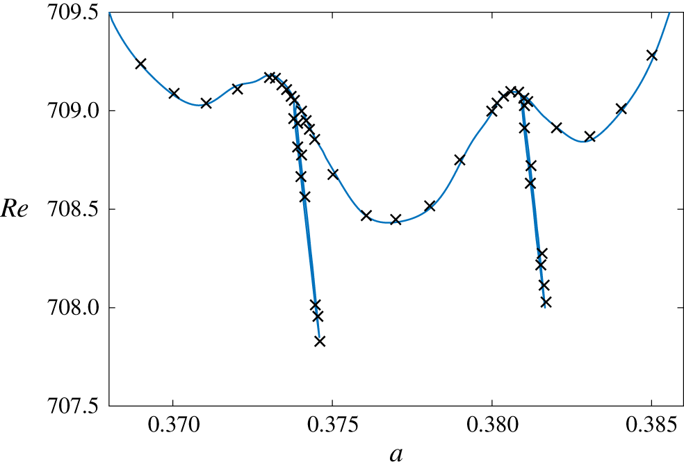
 $0.36\leqslant a\leqslant 0.39$. Figure 2 depicts the corresponding neutral stability curve obtained using the smaller valued wavenumber increment. Computations are plotted about the critical conditions for linear instability on a similar scale as those results presented in figure 3 of Blennerhassett & Bassom (Reference Blennerhassett and Bassom2002), which are included within the illustration using cross markers. The spikey protrusions are captured in detail and results are in excellent agreement with that given by the aforementioned authors with
 $(a_{c},Re_{c})=(0.375,707.84)$. Moreover, it is noted that in addition to the spikey features, the neutral stability curve is characterised by several bumps.
Neutral stability curve for the Stokes layer ( $\unicode[STIX]{x1D6FD}=0.5$) about the critical conditions for linear instability. Cross markers correspond to those results presented in Blennerhassett & Bassom (Reference Blennerhassett and Bassom2002).

4.2 Neutral stability curves
The above analysis was extended to the acceleration-skewed flow profiles given by (2.3). As those flows established for  $\unicode[STIX]{x1D6FD}\in [0,0.5]$ are the mirror images of those flows generated for
 $\unicode[STIX]{x1D6FD}\in [0.5,1]$, the subsequent study was limited to the latter parameter range. (For example, flows corresponding to
 $\unicode[STIX]{x1D6FD}=0.25$ and 0.75 are analogous, but with the acceleration and deceleration phases of the oscillatory motion flipped.) Additionally, the base flow (2.3) is dependent on the number of harmonics
 $N$. Thus, linear stability analysis was undertaken for
 $N\in [2,16]$ at step intervals of two; as
 $N$ increases the coefficient
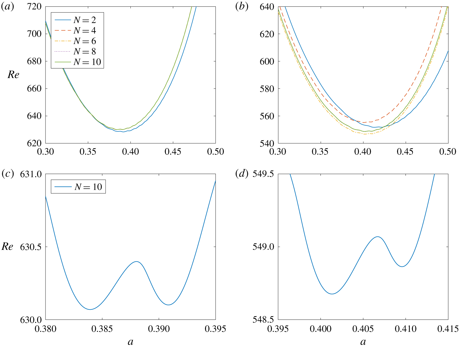
 $\unicode[STIX]{x1D6FE}_{n}$, given by (2.1b), decreases and stability calculations can be expected to approach an asymptotic limit. Figure 3 depicts neutral stability curves for those base flows established for
 $\unicode[STIX]{x1D6FD}=0.6$ and 0.75. Linear stability calculations were first computed at wavenumber intervals
 $\unicode[STIX]{x0394}a=10^{-3}$, with the corresponding neutral curves plotted in figures 3(a) and 3(b). In each instance, solutions are plotted for harmonics
 $N\in [2,10]$. Neutral curves matching to
 $\unicode[STIX]{x1D6FD}=0.6$ are, to graphical accuracy, unchanged for
 $N>4$, while stability calculations for
 $\unicode[STIX]{x1D6FD}=0.75$ appear to be unaffected by harmonics
 $N>8$. Furthermore, the critical Reynolds number
 $Re_{c}$ for the onset of linearly unstable behaviour is significantly less than that found for the symmetric Stokes layer;
 $Re_{c}\approx 630$ and
 $Re_{c}\approx 549$ for the respective flows
 $\unicode[STIX]{x1D6FD}=0.6$ and
 $\unicode[STIX]{x1D6FD}=0.75$.
Neutral stability curves for (a,c)  $\unicode[STIX]{x1D6FD}=0.6$; (b,d)
 $\unicode[STIX]{x1D6FD}=0.75$ and variable
 $N$.

In an attempt to resolve any spike-like features along the two sets of neutral stability curves, wavenumber increments  $\unicode[STIX]{x0394}a=10^{-5}$ were applied to the two flows based on
 $N=10$ harmonics. Figures 3(c) and 3(d) depict the corresponding neutral curves about the critical conditions for linear instability, for the respective flows
 $\unicode[STIX]{x1D6FD}=0.6$ and
 $\unicode[STIX]{x1D6FD}=0.75$. Although the wavenumber step size has been reduced, spikey protrusions matching to stationary waves were not located. However, the bumpy behaviour found for the Stokes layer has become more prominent. Both neutral curves display two distinct local minima, with critical conditions for linear instability located about one of these minima.
The absence of spikey structures in those plots illustrated in figure 3 is explained by considering the effect of acceleration skewness on the Floquet exponent  $\unicode[STIX]{x1D707}$. For the symmetrically oscillating Stokes layer, Floquet modes
 $\unicode[STIX]{x1D707}$ appear as a complex conjugate pair
 $\unicode[STIX]{x1D707}_{r}\pm \text{i}\unicode[STIX]{x1D707}_{i}$, matching to left- and right-travelling disturbances with an identical growth rate. However, acceleration skewness destroys this symmetry and establishes an asymmetrically oscillating flow. Left- and right-travelling waves no longer develop with the same growth rate. This behaviour is comparable with that described in Thomas et al. (Reference Thomas, Bassom, Blennerhassett and Davies2011) that was concerned with the linear stability of oscillating Poiseuille flow in a channel. (A natural distinction between the two travelling waves is that the left-travelling wave propagates in the upstream direction, while the right-travelling wave convects along the downstream direction.)
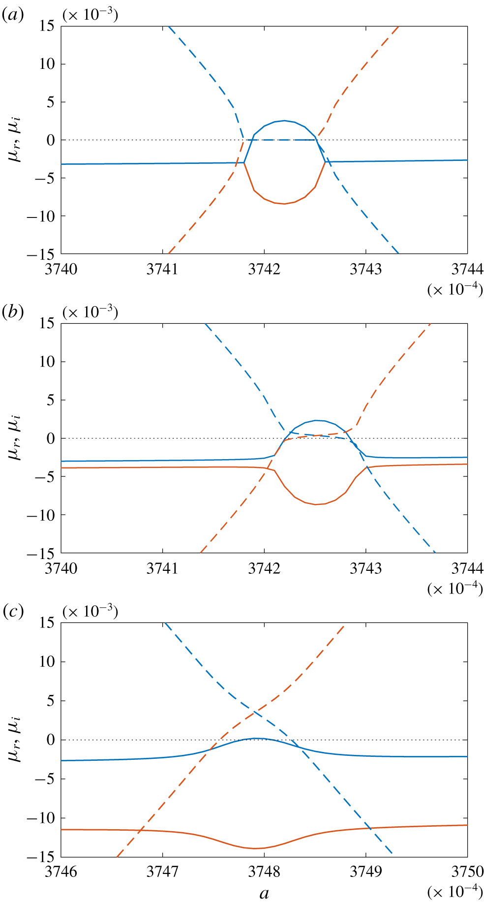
Figure 4 depicts the real and imaginary parts of the two Floquet modes (corresponding to the left- and right-travelling waves) as a function of the wavenumber  $a$ in the vicinity of a region where
 $\unicode[STIX]{x1D707}_{i}=0$, for base flows
 $\unicode[STIX]{x1D6FD}=0.5,0.5001$ and
 $0.501$. The real and imaginary parts of
 $\unicode[STIX]{x1D707}$ are respectively plotted using solid and dashed lines, while red and blue line types are matched to the left- and right-travelling disturbances. Results plotted in figure 4(a) correspond to the symmetric Stokes layer for
 $Re=708.4$. This particular Reynolds number was chosen as it passes through the spikey structures illustrated in figure 2, but is marginally less than the critical Reynolds number matching to the most unstable travelling wave;
 $Re_{c}=708.43$. For the wavenumber
 $a=0.374$, two stable travelling modes form a complex conjugate pair with identical growth rates
 $\unicode[STIX]{x1D707}_{r}$, but opposite sign values for
 $\unicode[STIX]{x1D707}_{i}$. As the wavenumber
 $a$ increases, the left- and right-travelling waves coalesce and stationary waves emerge on a finite range of
 $a$. Over this interval the two stationary waves have very different growth rates, with one mode becoming unstable. This behaviour matches the formation of the spike-like protrusions depicted in figure 2 for the symmetrically oscillating Stokes layer. For further increases in
 $a$, the two stationary waves are again both stable and reestablish the two stable travelling modes.
Variation of  $\unicode[STIX]{x1D707}_{r}$ (solid curves) and
 $\unicode[STIX]{x1D707}_{i}$ (dashed) with the wavenumber
 $a$ in the vicinity of a region where
 $\unicode[STIX]{x1D707}_{i}=0$. Red and blue line types depict results matching to left- and right-travelling waves. (a) An example for
 $\unicode[STIX]{x1D6FD}=0.5$ and
 $Re=708.4$; (b)
 $\unicode[STIX]{x1D6FD}=0.5001$ and
 $Re=708.35$; (c)
 $\unicode[STIX]{x1D6FD}=0.501$ and
 $Re=707.55$.

Similar depictions of the Floquet mode behaviour are shown in figures 4(b) and 4(c) for the parameter settings  $(\unicode[STIX]{x1D6FD},Re_{c})=(0.5001,708.35)$ and
 $(\unicode[STIX]{x1D6FD},Re_{c})=(0.501,707.55)$. These particular Reynolds numbers were again chosen as they correspond to values marginally less than the critical conditions for linear instability obtained using a wavenumber step size
 $\unicode[STIX]{x0394}a=10^{-3}$;
 $Re_{c}=708.40$ and
 $Re_{c}=707.59$ for the respective flows
 $\unicode[STIX]{x1D6FD}=0.5001$ and
 $\unicode[STIX]{x1D6FD}=0.501$. As a consequence of the wave asymmetry brought about by the acceleration skewness, the two travelling modes no longer form a complex conjugate pair. There are now distinct differences in the growth rates
 $\unicode[STIX]{x1D707}_{r}$, which are enhanced as
 $\unicode[STIX]{x1D6FD}$ increases. Furthermore, the imaginary parts
 $\unicode[STIX]{x1D707}_{i}$ are no longer reflected about the real axis. Acceleration skewness reduces the growth rate matching to the left-travelling wave, while the growth rate of the corresponding right-travelling wave remains marginally stable. Although not shown here, further increases in
 $\unicode[STIX]{x1D6FD}$ leads to considerably greater reductions in the growth rate of the left-travelling wave. (This behaviour is reversed for those flows established for
 $\unicode[STIX]{x1D6FD}<0.5$.) Marginally unstable waves develop on the wavenumber interval
 $0.3742<a<0.3743$ for the flow
 $\unicode[STIX]{x1D6FD}=0.5001$. Hence, a spike-like structure is expected to form along the neutral stability curve for this particular flow. However, the unstable modes on this interval are only stationary at one wavenumber
 $a$. Due to the asymmetry all other modes along this interval are now travelling waves. Furthermore, this pocket of instability diminishes as
 $\unicode[STIX]{x1D6FD}$ is increased to larger values, eventually receding from the stability plane altogether. Similar behaviour was observed about other locations where spikes formed for the symmetric Stokes layer. Thus, spike-like protrusions do not appear along the neutral stability curves for base flows
 $\unicode[STIX]{x1D6FD}\gtrapprox 0.5$ (and similarly
 $\unicode[STIX]{x1D6FD}\lessapprox 0.5$).
4.3 Critical conditions for linear instability
Critical conditions  $(Re_{c},a_{c})$ for linear instability are computed for a range of
 $\unicode[STIX]{x1D6FD}$ values and harmonics
 $N$. The critical Reynolds number
 $Re_{c}$ and wavenumber
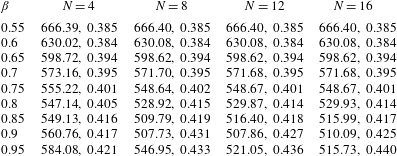
 $a_{c}$ are respectively quoted to two and three decimal places in table 1. Due to the absence of spike-like characteristics, stability calculations were based on a wavenumber step size
 $\unicode[STIX]{x0394}a=10^{-3}$. Computations corroborate the earlier observations that stability results are only marginally affected by harmonics
 $N>4$ and
 $N>8$ for the respective flows
 $\unicode[STIX]{x1D6FD}=0.6$ and
 $\unicode[STIX]{x1D6FD}=0.75$. Similar trends are observed for other acceleration-skewed flows. The magnitude of the coefficient
 $\unicode[STIX]{x1D6FE}_{n}$, given by (2.1b), decreases very quickly as
 $\unicode[STIX]{x1D6FD}$ approaches
 $0.5$. Hence, fewer harmonics are required to achieve the desired accuracy in the critical conditions. However, as
 $\unicode[STIX]{x1D6FD}$ approaches unity and the waveform adopts a sawtooth shape, a greater number of harmonics
 $N$ are required to correctly compute the onset of linear instability;
 $\unicode[STIX]{x1D6FE}_{n}$ decreases slowly and remains significant for larger valued harmonics. Indeed, results matching to
 $\unicode[STIX]{x1D6FD}=0.95$ have not converged for those cases considered herein. Hence, additional harmonics and further analysis are required to improve the stability calculations for this particular flow.
The current study was not extended to larger harmonics  $N$ due to computational constraints. As
 $N$ increases, the matrix
 $\unicode[STIX]{x1D63C}$ in (3.13) is more densely populated and, the speed and efficiency of the sparse-matrix eigensolver routines are greatly reduced. Hence, linear stability analysis was limited to harmonics
 $N\leqslant 16$. Nevertheless, stability calculations appear to have converged for those flows generated for
 $\unicode[STIX]{x1D6FD}\leqslant 0.9$.
Critical conditions  $Re_{c},a_{c}$ for linear instability.

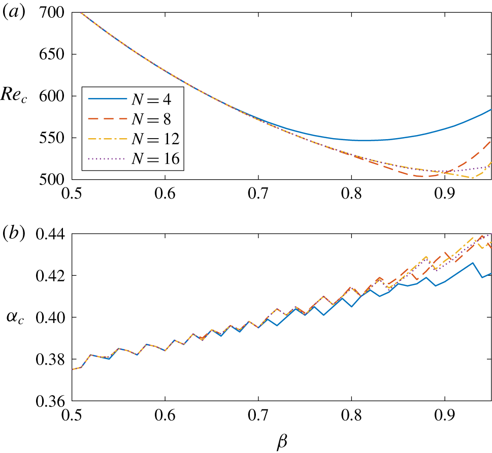
Critical conditions for linear instability as a function of  $\unicode[STIX]{x1D6FD}$. (a)
 $Re_{c}$; (b)
 $a_{c}$.

The critical Reynolds number  $Re_{c}$ and wavenumber
 $a_{c}$ for linear instability are plotted in figure 5 as functions of
 $\unicode[STIX]{x1D6FD}$. Calculations were computed at intervals
 $\unicode[STIX]{x0394}\unicode[STIX]{x1D6FD}=0.01$ and are presented for harmonics
 $N=4,8,12$ and 16. The value for
 $Re_{c}$, that is realised for sufficiently large harmonics
 $N$, decreases monotonically as
 $\unicode[STIX]{x1D6FD}$ is increased from 0.5 (Stokes layer) to 1 (sawtooth function). Thus, unstable behaviour appears earlier as the degree of acceleration skewness increases. Furthermore, the critical Reynolds number
 $Re_{c}$ can be crudely approximated by the following quadratic expression:
 $$\begin{eqnarray}Re_{c}\sim 922\unicode[STIX]{x1D6FD}^{2}-1787\unicode[STIX]{x1D6FD}+1370\quad \text{on }\unicode[STIX]{x1D6FD}\in [0.5,0.9].\end{eqnarray}$$
The plots of the critical wavenumber  $a_{c}$, depicted in figure 5(b), are non-smooth. As
 $\unicode[STIX]{x1D6FD}$ increases, the value for
 $a_{c}$ jumps at irregular but frequent intervals. This rather odd behaviour can be explained by referring back to those neutral curves depicted in figures 3(c) and 3(d). Neutral stability curves are bumpy with two (or more) local minima. Critical conditions for linear instability are located along one of these bumps. However, as
 $\unicode[STIX]{x1D6FD}$ increases, critical conditions for linear instability shift from one bump to another bump. Hence, non-smooth wavenumber profiles are obtained. Reducing the wavenumber step size was not found to affect this particular observation.
4.4 Eigenfunctions
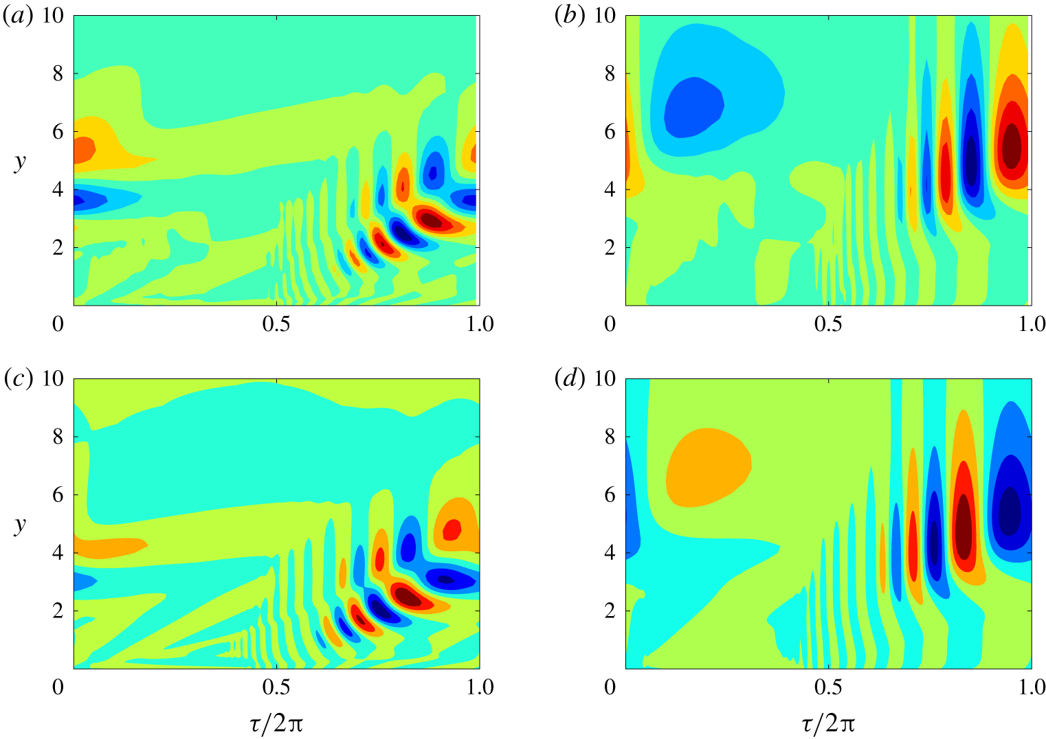
Contours of the real part of the vorticity  $\unicode[STIX]{x1D714}$ (plotted on the left) and streamfunction
 $\unicode[STIX]{x1D713}$ (right) are illustrated in figure 6 within the
 $(\unicode[STIX]{x1D70F},y)$-plane. Solutions are plotted for two neutral modes with the flow settings
 $(\unicode[STIX]{x1D6FD},Re)=(0.5,708.9)$ and
 $(\unicode[STIX]{x1D6FD},Re)=(0.75,553.4)$. In each instance the wavenumber
 $a=0.38$, while the corresponding values of
 $\unicode[STIX]{x1D707}_{i}$ are 0.1469 and 0.3493. Each solution has been normalised on its respective maximum complex-valued amplitude. Positive and negative valued contours are plotted in red and blue, respectively. Although the two sets of results are based on very different acceleration skewness settings, the respective structures of the vorticity and streamfunction are almost identical. Furthermore, they are consistent with those results presented by Blennerhassett & Bassom (Reference Blennerhassett and Bassom2002). (It is worth noting that due to the definition of the base flow, results shown here are shifted by a quarter period compared with those solutions depicted in the earlier study by Blennerhassett and Bassom.) For those flow conditions considered, disturbances appear within the boundary layer about time
 $\unicode[STIX]{x1D70F}=\unicode[STIX]{x03C0}$. Initially disturbances evolve with a high-frequency oscillation and grow along lines of constant
 $\unicode[STIX]{x1D70F}-y$; the streamfunction develops along one line, while the vorticity displays strong growth along two lines. Disturbances attain a maximum amplitude near the boundary layer edge, while further away from the wall the frequency of the oscillation decreases and the amplitude of the disturbance diminishes.
Contours of the real part of the vorticity  $\unicode[STIX]{x1D714}$ (a,c) and streamfunction
 $\unicode[STIX]{x1D713}$ (b,d) in the
 $(\unicode[STIX]{x1D70F},y)$-plane for (a,b)
 $\unicode[STIX]{x1D6FD}=0.5$ and
 $(Re,a,\unicode[STIX]{x1D707}_{i})=(708.9,0.38,0.1469)$; (c,d)
 $\unicode[STIX]{x1D6FD}=0.75$ and
 $(Re,a,\unicode[STIX]{x1D707}_{i})=(553.4,0.38,0.3493)$.

The above description of the vorticity and streamfunction was typical of many other flow conditions  $(Re,a)$ and acceleration skewness settings
 $\unicode[STIX]{x1D6FD}$. However, one subtle difference emerged as
 $\unicode[STIX]{x1D6FD}$ was raised above a value of 0.5. For the symmetric Stokes layer, disturbances were observed to originate about either
 $\unicode[STIX]{x1D70F}=0$ or
 $\unicode[STIX]{x1D70F}=\unicode[STIX]{x03C0}$. As noted by Blennerhassett & Bassom (Reference Blennerhassett and Bassom2002) this coincides with the wall velocity (2.1a) being zero. Furthermore, Thomas et al. (Reference Thomas, Davies, Bassom and Blennerhassett2014) showed that disturbances grew rapidly after the shear stress at the wall
 $U_{B}^{\prime }(0,\unicode[STIX]{x1D70F})$ changed sign; see figure 1 of their paper. Disturbances propagate to the right (left) when the shear stress reverses from a negative (positive) to a positive (negative) value, which occurs about
 $\unicode[STIX]{x1D70F}=3\unicode[STIX]{x03C0}/4+2\unicode[STIX]{x03C0}k$ (
 $=7\unicode[STIX]{x03C0}/4+2\unicode[STIX]{x03C0}k$) for the base flow (2.3) and
 $k\in \mathbb{Z}$. Hence, for the Stokes layer, disturbances can be expected to propagate in both the left and right spatial directions. This behaviour was confirmed by Thomas et al. (Reference Thomas, Davies, Bassom and Blennerhassett2014) who undertook a numerical study on the impulse response of disturbances in the spatial–temporal plane. Disturbances took the form of wavepackets that convected in both the left- and right-directions, leading to the formation of a family-tree-like structure.
For those flows established for an acceleration skewness parameter  $\unicode[STIX]{x1D6FD}>0.5$, disturbances were only ever observed to emanate about
 $\unicode[STIX]{x1D70F}=\unicode[STIX]{x03C0}$. This particular observation was tested for many flow conditions
 $(\unicode[STIX]{x1D6FD},Re,a)$ and in each instance the disturbance emerged about the mid-point of the wall motion. Thus, disturbances to flows
 $\unicode[STIX]{x1D6FD}>0.5$ can be expected to propagate to the right only, which coincides with the direction that the wall acceleration achieves a maximum absolute value. (It is noted that there are an infinite number of flow settings and that there may be some cases, not tested, that establish a disturbance about
 $\unicode[STIX]{x1D70F}=0$ that propagate to the left.) This behaviour is reversed for those flows generated for
 $\unicode[STIX]{x1D6FD}<0.5$. Disturbances emerge about
 $\unicode[STIX]{x1D70F}=0$ and convect to the left.
5 Conclusions
A linear stability study has been undertaken for those time-periodic flows established by an acceleration-skewed oscillating planar wall. Acceleration skewness was implemented using the van der A et al. (Reference van der A, O’Donoghue, Davies and Ribberink2011) model that is quantified by an acceleration skewness parameter  $\unicode[STIX]{x1D6FD}$ and the number of harmonics
 $N$. The classical Stokes layer, that was first shown to be linearly unstable by Blennerhassett & Bassom (Reference Blennerhassett and Bassom2002), is realised when the acceleration and deceleration phases of the wave motion are identical. The linear stability of the asymmetrically oscillating flows was then obtained by increasing the number of harmonics
 $N$ in the base flow (2.3). For sufficiently large
 $N$, stability calculations were computed accurately and unchanged by further increments in
 $N$. Acceleration skewness was found to reduce the critical conditions for the onset of linear instability. Hence, acceleration skewness is destabilising. In the context of waves propagating in coastal seas, this would suggest that an asymmetrically skewed wave will become unstable and turbulent before a symmetrically oscillating wave.
A detailed study of the neutral stability curve has shown that the spike-like structures found for the symmetric Stokes layer (that correspond to stationary waves), diminish as the degree of acceleration skewness is increased. This was as a consequence of the wave asymmetry that establishes left- and right-travelling waves with different growth rates. Furthermore, disturbances were shown to propagate to the right (left) when the acceleration skewness parameter  $\unicode[STIX]{x1D6FD}>0.5$ (
 ${<}0.5$), which coincides with the direction that the wall acceleration achieves a maximum absolute value.
The Reynolds numbers found here for the onset of linearly unstable behaviour are significantly greater than those values modelled in the numerical study by Scandura et al. (Reference Scandura, Faraci and Foti2016). For the flow engineered by the acceleration skewness parameter  $\unicode[STIX]{x1D6FD}=0.75$, Scandura and co-workers observed turbulent structures for Reynolds numbers as low as
 $Re=375$, while linear instability emerges for
 $Re>548$. Thus, the Floquet instabilities investigated in this paper are unlikely to be observed in either numerical studies that include turbulence effects or in experiments. This behaviour is comparable with the theoretical–experimental discrepancies that have been reported for the symmetric Stokes layer. Many experimental investigations on the Stokes layer in a channel or pipe observed unstable behaviour for
 $Re<300$ (Merkli & Thomann Reference Merkli and Thomann1975; Hino, Sawamoto & Takasu Reference Hino, Sawamoto and Takasu1976; Clamen & Minton Reference Clamen and Minton1977; Akhaven, Kamm & Shapiro Reference Akhaven, Kamm and Shapiro1991; Eckmann & Grotberg Reference Eckmann and Grotberg1991), which is considerably less than that reported by Blennerhassett & Bassom (Reference Blennerhassett and Bassom2002) for the onset of linear instability. Several explanations for the large variations between theory and experiments have been postulated, including geometry (Blennerhassett & Bassom Reference Blennerhassett and Bassom2006; Thomas, Bassom & Blennerhassett Reference Thomas, Bassom and Blennerhassett2012), quasi-steady instabilities (Cowley Reference Cowley, Dwoyer and Hussaini1987; Hall Reference Hall2003; Luo & Wu Reference Luo and Wu2010) and wall roughness (Vittori & Verzicco Reference Vittori and Verzicco1998). More recently, Thomas et al. (Reference Thomas, Blennerhassett, Bassom and Davies2015) suggested that imperfections in the experimental apparatus could introduce some low level noise that establishes the premature onset of unstable behaviour. It was shown that high-frequency modulation at amplitudes near 1 % of the wall motion could reduce the critical Reynolds number for linear instability by more than a half, bringing the theoretical observations in line with those values reported experimentally. Similar explanations for any differences between theory and experiments may also be applicable to the acceleration skewness flows modelled in this study.
Acknowledgements
The author is grateful to the referees for several suggestions which have led to a much improved paper.
Declaration of interests
The author reports no conflict of interest.
Appendix A. Integral operators
Integral operators  $\unicode[STIX]{x1D644}$ and
 $\unicode[STIX]{x1D646}$ are defined as
 $$\begin{eqnarray}\unicode[STIX]{x1D644}q_{m}(\unicode[STIX]{x1D702})=\int ^{\unicode[STIX]{x1D702}}\int ^{\unicode[STIX]{x1D702}^{\prime }}q_{m}(\unicode[STIX]{x1D702}^{\prime \prime })\,\text{d}\unicode[STIX]{x1D702}^{\prime }\,\text{d}\unicode[STIX]{x1D702}^{\prime \prime },\end{eqnarray}$$
and
 $$\begin{eqnarray}\unicode[STIX]{x1D646}q_{m}(\unicode[STIX]{x1D702})=\frac{1}{l^{2}}\left\{\unicode[STIX]{x1D702}^{4}q_{m}(\unicode[STIX]{x1D702})-6\int ^{\unicode[STIX]{x1D702}}{\unicode[STIX]{x1D702}^{\prime }}^{3}q_{m}(\unicode[STIX]{x1D702}^{\prime })\,\text{d}\unicode[STIX]{x1D702}^{\prime }+6\int ^{\unicode[STIX]{x1D702}}\int ^{\unicode[STIX]{x1D702}^{\prime }}{\unicode[STIX]{x1D702}^{\prime \prime }}^{2}q_{m}(\unicode[STIX]{x1D702}^{\prime \prime })\,\text{d}\unicode[STIX]{x1D702}^{\prime }\,\text{d}\unicode[STIX]{x1D702}^{\prime \prime }\right\}.\end{eqnarray}$$
Applying these operators to the odd Chebyshev series (3.9) leads to the following tridiagonal and pentadiagonal matrices:
 $$\begin{eqnarray}\unicode[STIX]{x1D644}\mathop{\sum }_{j=1}^{J}q_{m,j}T_{2j-1}=aT_{0}+bT_{1}+\mathop{\sum }_{j=2}^{J+1}{\displaystyle \frac{1}{8}}\left\{{\displaystyle \frac{q_{m,j-1}}{(2j-1)(j-1)}}-{\displaystyle \frac{q_{m,j}}{j(j-1)}}+{\displaystyle \frac{q_{m,j+1}}{j(2j-1)}}\right\}T_{2j-1},\end{eqnarray}$$
and
 $$\begin{eqnarray}\displaystyle \displaystyle \unicode[STIX]{x1D646}\mathop{\sum }_{j=1}^{J}q_{m,j}T_{2j-1} & = & \displaystyle cT_{0}+dT_{1}+\mathop{\sum }_{j=2}^{J+1}\frac{1}{16l^{2}}\big\{{\mathcal{A}}_{-2}q_{m,j-2}+{\mathcal{A}}_{-1}q_{m,j-1}\nonumber\\ \displaystyle & & \displaystyle +\,{\mathcal{A}}_{0}q_{m,j}+{\mathcal{A}}_{1}q_{m,j+1}+{\mathcal{A}}_{2}q_{m,j+2}\big\},\end{eqnarray}$$
where the arbitrary constants  $a,b,c,d$ arise from the double indefinite integration, while coefficients
 ${\mathcal{A}}_{\ast }$ are defined as
 $$\begin{eqnarray}\displaystyle & \displaystyle {\mathcal{A}}_{-2}=1-{\displaystyle \frac{6}{2j-1}}+{\displaystyle \frac{3}{(j-1)(2j-1)}}, & \displaystyle\end{eqnarray}$$
 $$\begin{eqnarray}\displaystyle & \displaystyle {\mathcal{A}}_{-1}=1-{\displaystyle \frac{12}{2j-1}}+{\displaystyle \frac{3}{j(j-1)(2j-1)}}, & \displaystyle\end{eqnarray}$$
 $$\begin{eqnarray}\displaystyle & \displaystyle {\mathcal{A}}_{0}=6-{\displaystyle \frac{3}{j(j-1)}}, & \displaystyle\end{eqnarray}$$
 $$\begin{eqnarray}\displaystyle & \displaystyle {\mathcal{A}}_{1}=4+{\displaystyle \frac{12}{2j-1}}-{\displaystyle \frac{3}{j(j-1)(2j-1)}}, & \displaystyle\end{eqnarray}$$
 $$\begin{eqnarray}\displaystyle & \displaystyle {\mathcal{A}}_{2}=1+{\displaystyle \frac{6}{2j-1}}+{\displaystyle \frac{3}{j(2j-1)}}, & \displaystyle\end{eqnarray}$$
 $j\in [1,J]$.