Many-body potentials

Atomic-scale computer simulations of materials such as Monte Carlo (MD) and molecular dynamics (MD) rely on a prescription of the energy in terms of the atomic positions, which is often referred to as the interatomic potential. In the early 1980s, however, the typical interatomic potential models used were pair potentials. As mentioned in the introductory article by Sinnott and Brenner in this issue of MRS Bulletin, pair potential models have well-known limitations in the description of crystalline solids. Further, the theoretical framework of pair potentials is based on bulk materials and so could only be applied to systems that did not contain surfaces and interfaces. Finally, there was an increasing interest in models that went beyond qualitative features and represented specific materials systems.

Multiple approximations were proposed during the first half of the 1980s for the energy of a metallic system that provided a means to describe the energy of an inhomogeneous system. While the physical motivations differed, the energy expressions had similar mathematical forms. In particular, the energy expressions can be written in the formReference Daw, Foiles and Baskes^1, Reference Carlsson, Ehrenreich and Turnbull²

(1)

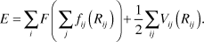
In this expression, i and j are indices referring to the atoms, R_ij is the separation between atoms i and j, V is a pair interaction between atoms i and j, and the functions f and F have interpretations that depend on the different models as discussed later.

This form has one significant advantage: it can be applied to inhomogeneous problems. The sidebar discusses the consequences of this form for the energy. Here, we will briefly outline the reasoning that led various authors to propose Equation 1. In the process, the physical interpretation of the various terms in Equation 1 will be described. As will be seen, these interpretations of the terms are different.

One route to Equation 1 starts with the concepts of the quasiatom theory of Stott and ZarembaReference Stott and Zaremba³ and the effective medium theory of Norskov.Reference Nørskov⁴ These theories assert that the energy of light impurity atoms such as hydrogen is largely determined by the energy to embed that impurity into the local electron density, the embedding energy. Daw and BaskesReference Daw and Baskes^5, Reference Daw and Baskes⁶ extended this idea in a study of nickel and palladium hydrides by applying the embedding energy concept to both the host metal atoms as well as the impurities. This line of development led to the embedded-atom method (EAM)Reference Daw, Foiles and Baskes¹ potentials.

From the EAM perspective, the function F in Equation 1 is the embedding energy. The argument of F represents the local electron density in which the atom is placed. This is computed by a superposition of atomic-like electron densities. Thus, the functions f_ij are the electron density from atom j at the location of atom i. The remaining terms in the energy are contained in the pair interaction term V.

Another route to Equation 1 starts with a tight-binding description of the electronic structure of a solid. A major component of the bonding of a solid results from the broadening of atomic energy levels into bands. The strength of this bonding for a given band filling scales with the width of the band that is formed. The width can be estimated from the second moment of the band. The second moment can, in turn, be computed in a tight-binding calculation from the sum of the square of the Hamiltonian matrix elements between an atom and all of its neighbors. This relates the estimation of the bonding energy to a pairwise sum over neighbors.

Finnis and SinclairReference Finnis and Sinclair⁷ used this reasoning to propose a set of potentials for the transition metals. In this case, the function F is proportional to a square root since the bonding energy scales with the square root of the second moment. The functions f_ij now correspond to the square of the Hamiltonian matrix elements between the atoms i and j. The pair potential term V incorporates the non-band-structure energy terms of a tight binding model.

A third route to Equation 1 relies on a simple physical argument. In the framework of constant volume pair potentials, there is an implicit energy term that depends on the overall density, but this is problematic when an average density cannot be determined. Summing a finite-range and decreasing weight function over the neighbors of each atom provides a measure of the local average density. The first term of Equation 1 in this picture is the density dependent energy as a function of this measure of the local density, and the second term is the usual pair potential term.

One early example of such an approach is the glue model.Reference Ercolessi, Parrinello and Tosatti⁸ In this approach, the function f_ij is the weight function used to estimate the local density, and F is the structure independent portion of the energy that corresponds to that measure of the density.

In practice, most of these methods proceed by adjusting the various functions to fit the predictions of the model to a database of material properties. The choice of the forms of the functions is guided by the physical interpretation. In the case of the function f_ij, all of the motivations suggest that it should be a decreasing function of distance. Both the embedding argument and the second moment argument indicate that the function F should have a positive curvature. Thus these various approaches tend to be rather similar in their practical application despite the different physical arguments that led to them. The exception is that the treatment of alloys is different in the second-moment tight-binding approaches than in the EAM approaches. For the EAM approaches, the term f_ij only depends on the species of atom j, while it depends on the species of both atoms i and j in the second-moment tight binding approaches.

There can be significant differences between potentials developed using these approaches that nominally describe the same material. These differences have two origins. First, note that if the embedding function, F, is linear, the first term in Equation 1 is just another pair potential. Thus, some of the pair-like energy contributions can move between these two terms and yield identical results. The second source of differences results from the details of the process of fitting the potentials: different functional forms for the various functions as well as different fitting data. As a result, there can be significant differences in how well particular potentials within this class will represent the properties of interest for a given material.

Contemporary applications

Potentials of this type have been around for about 30 years; therefore, it is natural to ask whether this approach is still of value. While these approaches incorporate some key aspects of metallic binding, the approximations are still rather severe. For example, this class of potentials does not incorporate any angular dependence in the interactions that would be expected in systems where there is some covalent character to the bonding.Reference Daw, Foiles and Baskes¹ As discussed later and in other articles in the issue, other forms of potentials have been proposed. These newer potentials have the possibility of incorporating a better description of the bonding, but at the price of increased computational cost, sometimes by orders of magnitude. With the increase of computing power, these more expensive methods are now feasible for a wide range of problems and are seeing increased use.

Despite the advent of new approaches, the EAM type of potentials is still an important tool for materials simulation. The optimal choice of interatomic potential depends on the problem and the type of information that is required. In some problems, highly accurate descriptions that incorporate the subtle differences between materials are required. An example would be the core structure of screw dislocations in bcc metals. Different potentials predict different structures, and these differences have implications for the flow response of the material. In this case, highly quantitative potentials are needed, and the modest size of the simulations allows for expensive potentials, possibly even ab initio approaches, to be used. There are other problems that are dominated by complexity. In these cases, one needs to study a combination of very large dynamic systems and/or a large number of systems. Such problems require computationally efficient potential models that capture the essential physics. It is for this latter class of problems that simpler and efficient approaches such as EAM continue to be the most reasonable approach.

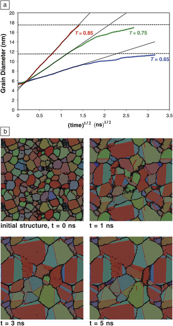
Recent work on grain growth in metals and its connection to the mobility of the grain boundary network represents one such example. Holm and FoilesReference Holm and Foiles⁹ simulated grain growth during the annealing of an atomic-level realization of a nanocrystalline grain structure. Snapshots of slices through such a simulation are shown in Figure 1. In this figure, the shading of the atoms reflects the local crystallographic orientation. These 3D simulations contained about 5 million atoms and considered times up to 10 ns. As such, these simulations are well within the range of current computer power for simple potentials such as EAM but would be prohibitive for more complex interaction models.

Figure 1.

Molecular dynamics simulations of grain growth in polycrystalline nickel. (a) Grain growth kinetics for individual simulations at three homologous temperatures (T). Black lines show normal growth kinetics with a grain diameter proportional to the square root of time; dashed lines indicate the stagnant grain size predicted by mesoscale simulations. (b) Time evolution of a slice through the 3D system for T = 0.75 T _melting at 0, 1, 3, and 5 ns. The regions shown are approximately 50 nm on a side. The atomic color scheme reflects local lattice orientation; red atoms are hexagonal close packed (hcp) coordinated (i.e., stacking faults, twins), and the black atoms are of unknown coordination (i.e., grain boundaries).Reference Holm and Foiles⁹

Figure 1 clearly shows the occurrence of grain growth. The short time scale for this curvature driven growth reflects the high temperature of the simulation, 0.75T _melting (T _melting is the melting temperature), as well as the high driving force due to the large curvature of the nanocrystalline grains. Figure 1a plots the average grain diameter as a function of the square root of time. There are a couple of interesting aspects of these curves. The curvature driven grain growth is expected to follow a square root of time dependence. The initial behavior in this curve is not physical since the initial grain structure was not equilibrated. After the initial transient of about 20 picoseconds, the grain diameters increase with the expected parabolic dependence for a significant length of time. Some researchers had suggested that nanocrystalline grain growth would follow different kinetics due to the increased influence of triple junctions on the dynamics.Reference Holm and Foiles⁹ These results in Figure 1 indicate that the growth follows normal kinetics for a period of time.

Another interesting observation is that after a period of normal growth kinetics, the growth slows at the lower two temperatures, as seen by the leveling off of the curves for T = 0.65 and T = 0.75. Holm and FoilesReference Holm and Foiles⁹ explained this behavior is a result from the presence of two classes of grain boundaries: mobile and essentially immobile. The relative populations of these two classes of boundaries depend on the temperature. It was hypothesized that this effect leads to the experimentally observed ultimate slowing of grain growth seen in high purity materials.

The existence of these two classes of boundaries was deduced from a molecular dynamics study of the mobility of 388 grain boundaries by Olmsted et al.Reference Olmsted, Holm and Foiles¹⁰ This study again required computationally efficient potentials. While the simulation cells required for examining the structure and mobility of the grain boundaries are of modest size, this study required tens of thousands of simulations to both determine the structure of the boundaries and examine their mobility as a function of temperature.

Simulations of stress evolution during thin-film deposition also demonstrate how simulations with this class of potentials can reveal important insights into the underlying mechanisms. In the case of Volmer-Weber growth,Reference Pao, Foiles, Webb, Srolovitz and Floro¹¹ the film forms in three stages: isolated islands nucleate and grow, nearby islands coalesce, and the continuous film thickens. In systems with high surface mobility, film stress measurements show that these stages typically correspond to compressive, tensile, and finally compressive stress evolution. Due to the need to be able to control film stress during growth, there has been extensive work to understand the mechanisms that lead to these stress responses.

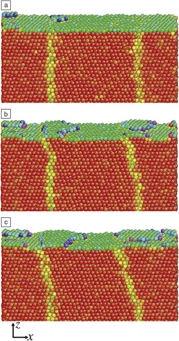
Atomic-scale simulations have been used to examine all of these stages. In particular, Pao et al.Reference Pao, Foiles, Webb, Srolovitz and Floro¹¹ used MD simulations to understand the compressive stress evolution during the growth of the film. MD simulations of deposition on a thin film of Ni with grain boundaries intersecting the surface showed the generation of compressive stress similar to experiment. Snapshots of the resulting films are shown in Figure 2. By following the motion of the individual atoms, they observed that some of the adatoms were incorporated into the grain boundary. This net mass flow into the film was then correlated with the compressive stress that was generated. Chason et al.Reference Chason, Sheldon, Freund, Floro and Hearne¹² earlier proposed the basic mechanism of adatoms incorporating into grain boundaries and producing compressive stress. The value that the simulation study provided was to demonstrate that the spontaneous incorporation of adatoms into the grain boundaries was in fact a realistic and viable mechanism.

Figure 2.

Simulation snapshots during the deposition of Ni onto a Ni thin film intersected by a grain boundary at deposited coverages of (a) 0.14, (b) 0.36, and (c) 0.49 monolayers. The shading of the atoms reflects the degree of deviation from a bulk-like environment, with red being bulk-like and blue being the least bulk-like. The results show how adatoms incorporate in the grain boundaries, which appear as yellowish regions.Reference Pao, Foiles, Webb, Srolovitz and Floro¹¹

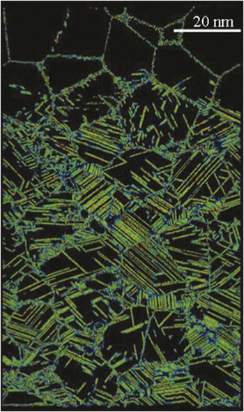
In the two prior examples, one of the challenges was using simulations on the molecular dynamics time scale of nanoseconds to understand processes that occur on much slower time scales. There are phenomena where the inherent time scales are on the order of nanoseconds, and the complexity arises from structures that are created or evolve. One such problem is the response of materials to shock loading, such as the work by Bringa et al.Reference Bringa, Caro, Wang, Victoria, McNaney, Remington, Smith, Torralva and Van Swyhenhoven^13, Reference Bringa, Rosolankova, Rudd, Remington, Wark, Duchaineau, Kalantar, Hawreliak and Belak¹⁴ on the shock deformation of fcc metals. The shock is simulated using a computational piston to drive the atoms at one end of the sample in a manner similar to experimental shock studies. Large simulation cells on the order of 350 million atoms were used to capture the complex three-dimensional dislocation structures that are produced. This work provides insight into the detailed mechanisms of dislocation generation and strength changes during the shock process. It is possible to elucidate the role of preexisting defects, either dislocation loops or initial nanocrystalline structures, on the evolution of the system, as seen in Figure 3. Further, the details of the kinetics of the dislocation nucleation, motion, and hardening can be observed. These results can be compared with the current generation of shock experiments. A recent article by Rudd et al.Reference Rudd, Germann, Remington and Wark¹⁵ discussed how microscopic models are beginning to be able to predict macroscopic properties such as plastic flow, and experimental capabilities are becoming available that will be able to probe the response at similar scales.

Figure 3.

A snapshot of a simulation of shock propagation through a nanocrystalline metal. Only a thin slab is shown. The shock has traveled for 30 ps from bottom to top producing a high density of partial dislocations together with perfect dislocations and nanotwins. Reprinted with permission from Reference Reference Bringa, Caro, Wang, Victoria, McNaney, Remington, Smith, Torralva and Van Swyhenhoven13. ©2005, American Association for the Advancement of Science.

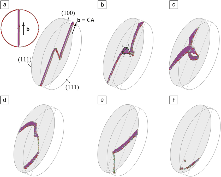
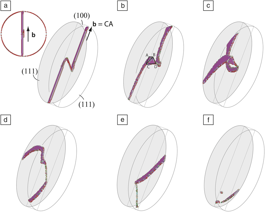
The previous examples utilize the ability of molecular dynamics simulations to predict the evolution of a system. Another use of molecular dynamics simulations is as a test bed for theoretical ideas. The recent work by Weinberger and CaiReference Weinberger and Cai¹⁶ on Lomer-Cottrell (LC) jogs, pinning points created from the interaction of two dislocations, in Ni nanopillars as a model fcc material demonstrates the value of such an approach. Experiments on nanopillars show that the flow stress increases as pillar size decreases. Two competing mechanisms have been proposed for this behavior: dislocation starvationReference Greer and Nix¹⁷ (the absence of dislocations in the small volume of a nanopillar) and single arm sourcesReference Rao, Dimiduck, Parthasarathy, Uchic, Tang and Woodward¹⁸ (a dislocation attached to a pinning point). The single arm source model requires strong pinning points. Lee and NixReference Lee and Nix¹⁹ proposed that LC jogs could provide the required pinning points. Weinberger and Cai performed simulations of evolution of a dislocation with an LC jog in a nanopillar. The results, depicted in Figure 4, of the evolution of the jog under stress show that the LC jogs do not form strong pinning points. Instead, the jog is able to rearrange such that it can move out of the nanopillar. This work demonstrates that LC jogs cannot be the strong pinning points required for single arm sources in nanopillars and more generally provides an example of how simulations can be used to evaluate theoretical explanations.

Figure 4.

The operation of a single arm source created from a Lomer-Cottrell jog in a 30 nm diameter nickel nanopillar. (a) The initial configuration of the source including an end-on view. (b) The extended node readily forms as predicted from geometrical considerations. (c) The arms rotate past each other on their {1 1 1} planes. (d) The jog rotates on its {1 0 0} plane, eliminating the extended node and forming a constricted jog. (e) The dislocation structure drifts along the {1 0 0} plane and (f) leaves the nanopillar. The structural notation in capital letters refer to the Thompson tetrahedron notation for dislocations.Reference Weinberger and Cai¹⁶b, Burgers vector.

Subsequent approaches

As discussed earlier, it is critical that the second derivative of the embedding function be positive. A positive curvature results in decreased bond energy and increased bond length with increasing coordination, as is observed in all materials. A second result of a positive curvatureReference Daw and Baskes⁶ is that the elastic constant ratio C ₁₂ /C ₄₄ > 1. Unfortunately, a large class of materials (e.g., Si, which has a diamond cubic ground state crystal structure) has C ₁₂ /C ₄₄ < 1. The covalent bonding in these materials is typified by “angular” bonding, hence there are angular forces. Baskes and co-workersReference Baskes^20–Reference Baskes²² modified the EAM to create a modified embedded atom method (MEAM) by including additional terms in the calculation of the background electron density. The addition of what were called “partial” electron densities creates the angular bonding and forces necessary to describe covalent materials.

There are numerous examples of calculations of semiconductor materials and alloys using the MEAM. Calculations as diverse as the behavior of Si ad-dimers,Reference Baskes²³ crack propagation speeds for brittle fracture in Si,Reference Swadener, Baskes and Nastasi²⁴ radiation damage in SiC,Reference Huang, Ghoniem, Wong and Baskes²⁵ surface segregation of bimetallic nanoparticles of Pt with Ni, Re and Mo,Reference Wang, Van Hove, Ross and Baskes²⁶ and phase transformation temperatures and thermodynamic properties of SnReference Ravelo and Baskes²⁷ all showed good agreement with experiment. One of the most impressive applications of MEAM was the development by Baskes and co-workersReference Baskes, Muralidharan, Stan, Valone and Cherne²⁸ of potentials for alloys of the highly complex f-electron material Pu with Ga. These potentials are able to reproduce the stability of the six crystalline phases and the liquid phase of Pu. MEAM Pu predicts the observed anomalously low melting point, the volume contraction upon melting, and the fact that the close-packed δ-phase has the highest volume per atom of all observed phases. The Pu-Ga phase diagram is perhaps the most complicated of all binary phase diagrams. It contains 21 phases at atmospheric pressure. The MEAM potentials predict that all of the experimentally observed phases have low energies at 0 K, but the energetics of these phases do not agree quantitatively with the observed phase diagram. Prediction of this complex phase diagram is still beyond our current capabilities.

Another solution to the absence of angular forces in the EAM follows from the tight-binding description of bonding that led to the Finnis-Sinclair (FS) potentials. As discussed earlier, the FS potentials relate the binding strength to the second moment of the density of states. Higher moments of the density of states can also be determined by local summations of the hopping matrix elements (i.e., the electronic interactions between the two orbitals). For a given band filling, the higher moments provide additional information about the local bond strength. Thus, it is possible to relate the computation of the local moments to the local energetics and ultimately to an interatomic potential model. This line of reasoning led to the development of bond order potentials by Pettifor and co-workersReference Pettifor²⁹ and the model generalized perturbation theory potentials by Moriarty.Reference Moriarty³⁰ These approaches are reviewed and described in more detail in various review articles.Reference Finnis^31, Reference Moriarty, Benedict, Glosli, Hood, Orlikowski, Patel, Soderlind, Streitz, Tang and Yang³² The definitive examination of the core structure of dislocations in Mo and W by Gröger, Vitek, and co-workersReference Gröger, Bailey and Vitek^33–Reference Gröger and Vitek³⁵ represents a major achievement in applying the bond order potentials. There are two potential structures for the core of the screw dislocations in bcc metals, and the use of these modern potentials was needed to discriminate between these two possible structures. This work relates the dislocations to the mechanical properties, and a correct description of the screw dislocation core structure was essential to this effort.

Development of materials through computation requires prediction of the thermodynamics and kinetics of multi-component materials having potentially complex electronic structure and crystal structure. Since we are intrinsically interested in temperature dependent properties, prediction of accurate free energies is a necessity. However, first-principles methods take too long. There has been recent work aimed at developing interatomic potentials that faithfully reproduce first-principles data. This is a daunting task. Baskes and co-workersReference Baskes, Srinivasan, Valone and Hoagland³⁶ introduced the concept of multiple reference structures and reference paths. A reference path is a simple lattice distortion that connects two reference states and is critical for the prediction of kinetics. This multi-state method used MEAM as a base, but is by no means a concept limited to the MEAM functional form. In this work, a multi-state MEAM (MS-MEAM) model of Cu was developed using an extensive first principles database, and the model was able to reproduce the database exactly, but transferability to atomic environments not in the database was not quantitative. Bartók and co-workersReference Bartók, Payne, Kondor and Csányi³⁷ proposed another approach with a similar goal. They introduced a novel set of coordinates for the description of the local environment and then applied Gaussian process regression to interpolate the energies, forces, and stresses computed from first principles calculations. Their results indicated much better agreement with first principles data than more traditional approaches, but it was limited to cases close to the training data, the configurations used to parameterize the potentials.

Concluding remarks

The advent of multi-body potentials, such as the embedded-atom method (EAM), in the early 1980s allowed for the examination of a much wider range of materials problems. It also sparked tremendous efforts to develop more realistic models of interatomic interactions. Thus, the ability to model materials properties has increased dramatically.

A wide range of models are now available for interatomic interactions that span the spectrum from simple, computationally efficient but less accurate methods to complex, computationally expensive, but more accurate and transferable methods. Part of the art of materials simulations is the choice of where in this spectrum of methods a given calculation should be performed. There is no universal best answer. The optimal choice depends on the problem to be solved and the nature of the information that is desired. In the case of problems that are dominated by complexity, it is better to use a less accurate method, but one that is efficient enough to allow the examination of all of the inherent complexity. The example applications of the EAM discussed previously are in that category. Problems that require precise quantitative results, such as determinations of phase diagrams, will require the most accurate potentials available. The field is fortunate to have moved beyond the time when only simple models were available to a time where a spectrum of methods exists from which the most appropriate one for the problem at hand can be chosen.