



1 Introduction
When bubbles are released continuously from a submersed source, they entrain ambient fluid to form a multiphase bubble/fluid mixed plume and rise together driven by the bubble buoyancy. The interaction of bubble-driven multiphase plumes (also referred to as bubble plumes) with a stably stratified fluid environment plays a crucial role in many environmental and engineering flow problems. On the one hand, strong bubble-induced buoyancy fluxes can generate turbulent plumes that provide significant mixing for stratified fluid environments. For example, bubble plumes have been widely used for reservoir destratification and aeration systems (Wüest, Brooks & Imboden Reference Wüest, Brooks and Imboden1992; Asaeda & Imberger Reference Asaeda and Imberger1993; Lemckert & Imberger Reference Lemckert and Imberger1993; Schladow Reference Schladow1993). Bubble plumes have also been used to mix hot and toxic fluids in chemical engineering applications (Leitch & Daines Reference Leitch and Daines1989). On the other hand, stratification can cause fluid in the plume to peel off and form an annular plume that falls down along the outside of the inner plume, similar to a fountain. This peeling process and associated downward flow in the outer plume can lead to trapping of entrained fluid and weakly buoyant particles within the water layer. One such example with significant environmental impact is a multiphase hydrocarbon plume from underwater accidental oil well blowouts (Camilli et al. Reference Camilli, Reddy, Yoerger, Van Mooy, Jakuba, Kinsey, Mclntyre, Sylva and Maloney2010). The underwater trapping increases the opportunity for biodegradation of the oil droplets, but also significantly increases the difficulty in estimating the total oil leak rate based on the surface plume signal as well as predicting the oil plume surfacing location.
Direct measurement of plume statistics in natural environments is a very challenging task. A limited set of field data for multiphase plumes have been conducted (e.g. Johansen, Rye & Cooper Reference Johansen, Rye and Cooper2003; Camilli et al. Reference Camilli, Reddy, Yoerger, Van Mooy, Jakuba, Kinsey, Mclntyre, Sylva and Maloney2010; Socolofsky, Adams & Sherwood Reference Socolofsky, Adams and Sherwood2011; Weber et al. Reference Weber, Robertis, Greenaway, Smith, Mayer and Rice2012), providing valuable data for understanding the complex interactions between buoyant plumes and their environment. With controlled stratification conditions and available measurement techniques for obtaining detailed plume statistics, experiments in laboratory water tanks have played a vital role in understanding complex plume flow physics. For example, using shadowgraph visualization of coloured dyes, Asaeda & Imberger (Reference Asaeda and Imberger1993) were able to observe various representative types of bubble plume structure and correlate plume behaviour with several key plume parameters (also see e.g., Richards, Aubourg & Sutherland (Reference Richards, Aubourg and Sutherland2014), for a more recent shadowgraph based experiment). Socolofsky (Reference Socolofsky2001) (also see Socolofsky & Adams Reference Socolofsky and Adams2003, Reference Socolofsky and Adams2005) performed a series of laser-induced fluorescence (LIF) measurements for buoyant plumes driven by air bubbles or oil droplets, as well as for inverted plumes driven by settling sediments. Seol, Bryant & Socolofsky (Reference Seol, Bryant and Socolofsky2009) performed LIF measurements to study both the instantaneous and the mean plume structures. Obtaining quantitative velocity information is very challenging in the laboratory due to the difficulty in controlling the bubble size in salt stratification and the complexity of matching the index of refraction throughout the ambient stratification.
Besides experimental observations, one-dimensional integral plume models have been developed and widely used as a tool for predicting mean plume dynamics (e.g. McDougall Reference McDougall1978; Milgram Reference Milgram1983; Wüest et al. Reference Wüest, Brooks and Imboden1992; Asaeda & Imberger Reference Asaeda and Imberger1993; Crounse, Wannamaker & Adams Reference Crounse, Wannamaker and Adams2007; Socolofsky, Bhaumik & Seol Reference Socolofsky, Bhaumik and Seol2008). Integral plume models usually assume a self-similar cross-plume variation (e.g. top hat or Gaussian) for plume variables (Davidson Reference Davidson1986). By performing cross-plume integration with the self-similarity assumption, the three-dimensional conservation laws are reduced to a set of coupled one-dimensional ordinary differential equations. The computational cost of calculating the mean plume characteristics are thus significantly reduced. Associated with the reduction of dimension, additional closures are required to model the turbulent entrainment fluxes between the inner and outer plumes as well as the peeling flux from the inner plume at the origin of the outer plume. These fluxes are usually parameterized based on the primary variables of the integral model (i.e. the model solutions) (Turner Reference Turner1986), with model coefficients that usually require calibration based on experimental data (e.g. Morton, Taylor & Turner Reference Morton, Taylor and Turner1956; Papanicolaou & List Reference Papanicolaou and List1988; Asaeda & Imberger Reference Asaeda and Imberger1993; Wang & Law Reference Wang and Law2002; Carazzo, Kaminski & Tait Reference Carazzo, Kaminski and Tait2008).
In order to capture the three-dimensional mean structure of the plume, computational models based on Reynolds-averaged Navier–Stokes (RANS) equations have been developed and widely used in chemical engineering applications. RANS models rely on different closures, mostly the
 $k$
–
 ${\it\varepsilon}$
model, to parameterize turbulent transport (e.g. Becker, Sokolichin & Eigenberger Reference Becker, Sokolichin and Eigenberger1994; Sokolichin & Eigenberger Reference Sokolichin and Eigenberger1994; Pfleger & Becker Reference Pfleger and Becker2001; Zhang, Deen & Kuipers Reference Zhang, Deen and Kuipers2006; Tabib, Roy & Joshi Reference Tabib, Roy and Joshi2008). Unlike RANS models, large-eddy simulation (LES) models are able to directly resolve both large-scale and a range of intermediate-scale turbulent motions (depending on the grid resolution), and only require modelling of the unresolved subgrid-scale (SGS) turbulence effects. While the cost of LES is significantly higher than RANS, in recent years LES has gained in popularity in many scientific and engineering applications due to the continuously increasing computing power available. LES has been used to simulate multiphase plumes in several recent studies (e.g. Deen, Solberg & Hjertager Reference Deen, Solberg and Hjertager2001; Niceno, Dhotre & Deen Reference Niceno, Dhotre and Deen2008; Tabib et al.
Reference Tabib, Roy and Joshi2008; Dhotre et al.
Reference Dhotre, Deen, Niceno, Khan and Joshi2013; Fabregat et al.
Reference Fabregat, Dewar, Özgökmen, Poje and Wienders2015). Using various types of SGS closures, these LES models were able to capture instantaneous fine-scale flow structures which were missing in RANS models. Very recently, Yang, Chamecki & Meneveau (Reference Yang, Chamecki and Meneveau2014a
) and Yang et al. (Reference Yang, Chen, Chamecki and Meneveau2015) developed a hybrid LES model for simulating hydrocarbon plume dispersion in ocean turbulence. Using their LES model, Yang et al. (Reference Yang, Chamecki and Meneveau2014a
, Reference Yang, Chen, Chamecki and Meneveau2015) studied the complex dispersion phenomena of oil plumes released into the ocean mixed layer, and investigated the effects of various environmental mixing mechanisms such as shear turbulence, waves and Langmuir circulations.
In this study, the hybrid LES model developed by Yang et al. (Reference Yang, Chamecki and Meneveau2014a , Reference Yang, Chen, Chamecki and Meneveau2015) is adopted and modified to simulate bubble-driven buoyant plumes in vertically stratified ambient fluid. To validate the model and investigate the essential plume characteristics in a controlled environment, the key simulation parameters are chosen to be similar to those of the laboratory measurements of Seol et al. (Reference Seol, Bryant and Socolofsky2009). In the simulation, a bubble plume is released from a localized source and rises through a stratified fluid column. The strength of the flow stratification and bubble flow rate are kept the same as in the experiment. Various bubble rise velocities relative to the fluid velocity are considered and their effects on the plume characteristics are studied. Statistical analysis is performed to quantify both the instantaneous and averaged plume characteristics. The temporally and spatially resolved plume information from the LES serves as a useful dataset for assessing and improving one-dimensional integral plume models that play an important role in rapid engineering predictions when full simulation is not feasible. Using the LES data, a priori tests are conducted for the key model closures used in integral models (i.e. entrainment and peeling models). Moreover, the data provide useful insights for developing a new peeling flux model.
The remainder of this paper is organized as follows. The LES model and simulation set-up for the bubble-driven buoyant plume are introduced in § 2. In § 3, the concept of the integral plume model is reviewed. The instantaneous and averaged plume structures obtained from LES are presented in § 4. Based on the LES results, in § 5 the integral plume model formulation is reviewed and assessed, and a new continuous peeling model is proposed. Conclusions are presented in § 6.
2 Large-eddy simulation model of multiphase buoyant plume
2.1 Model description
In this study, we consider a buoyant plume driven by an air bubble column that rises through vertically stratified quiescent ambient water. This flow configuration mimics the typical laboratory set-up for studying multiphase buoyant plumes (e.g. Socolofsky & Adams Reference Socolofsky and Adams2005; Seol et al.
Reference Seol, Bryant and Socolofsky2009). Let
 $\boldsymbol{x}=(x,y,z)=(x_{1},x_{2},x_{3})$
with
 $x$
and
 $y$
being the horizontal coordinates and
 $z$
being the vertical coordinate, and let
 $\boldsymbol{u}=(u,v,w)=(u_{1},u_{2},u_{3})$
be the corresponding velocity components. Fluid motions in and around the buoyant plume are described by the three-dimensional incompressible filtered Navier–Stokes equations
 $$\begin{eqnarray}\displaystyle & \displaystyle \boldsymbol{{\rm\nabla}}\boldsymbol{\cdot }\widetilde{\boldsymbol{u}}=0, & \displaystyle\end{eqnarray}$$
 $$\begin{eqnarray}\displaystyle & \displaystyle \frac{\partial \widetilde{\boldsymbol{u}}}{\partial t}+\widetilde{\boldsymbol{u}}\boldsymbol{\cdot }\boldsymbol{{\rm\nabla}}\widetilde{\boldsymbol{u}}=-\boldsymbol{{\rm\nabla}}\widetilde{P}-\boldsymbol{{\rm\nabla}}\boldsymbol{\cdot }{\bf\tau}^{d}+\left(1-\frac{\widetilde{{\it\rho}}}{\langle \widetilde{{\it\rho}}\rangle _{h}}\right)g\boldsymbol{e}_{3}+\left(1-\frac{{\it\rho}_{b}}{{\it\rho}_{r}}\right)\frac{\widetilde{C}_{b}}{{\it\rho}_{b}}g\boldsymbol{e}_{3}. & \displaystyle\end{eqnarray}$$
Here, a tilde denotes a variable resolved on the LES grid,
 ${\it\rho}_{b}$
is the density of air bubble,
 ${\it\rho}_{r}$
is the reference water density,
 $\widetilde{{\it\rho}}$
is the resolved local water density,
 $\langle \widetilde{{\it\rho}}\rangle _{h}$
is the horizontally averaged water density,
 ${\bf\tau}=(\widetilde{\boldsymbol{u}\boldsymbol{u}}-\widetilde{\boldsymbol{u}}\widetilde{\boldsymbol{u}})$
is the subgrid-scale (SGS) stress tensor, with
 $\text{tr}({\bf\tau})$
being its trace and
 ${\bf\tau}^{d}={\bf\tau}-[\text{tr}({\bf\tau})/3]~\unicode[STIX]{x1D644}$
being its deviatoric part,
 $\unicode[STIX]{x1D644}$
is the identity tensor,
 $\widetilde{P}=\widetilde{p}/{\it\rho}_{r}+\text{tr}({\bf\tau})/3+|\widetilde{\boldsymbol{u}}|^{2}/2$
is the pseudo pressure, with
 $\widetilde{p}$
being the resolved dynamic pressure,
 $\widetilde{C}_{b}$
is the resolved mass concentration of air bubbles,
 $g$
is the acceleration of gravity, and
 $\boldsymbol{e}_{3}$
is the unit vector in the vertical direction. The four terms on the right-hand side of (2.2) are the pressure gradient force, the SGS term representing the effect of the unresolved small-scale fluid motions, the buoyancy force due to water density fluctuations, and the buoyancy force due to air bubble concentration, respectively. The two buoyancy terms are based on the Boussinesq approximation.
Following previous LES studies (e.g. McWilliams, Sullivan & Moeng Reference Mcwilliams, Sullivan and Moeng1997; Polton et al.
Reference Polton, Smith, Mackinnon and Tejada-Martinez2008; Kukulka et al.
Reference Kukulka, Plueddemann, Trowbridge and Sullivan2010), a linear relation is assumed between the water density
 ${\it\rho}$
and the temperature
 ${\it\theta}$
, i.e.
 $$\begin{eqnarray}{\it\rho}={\it\rho}_{r}[1-{\it\alpha}({\it\theta}-{\it\theta}_{r})],\end{eqnarray}$$
where
 ${\it\alpha}=2\times 10^{-4}~\text{K}^{-1}$
is the thermal expansion coefficient and
 ${\it\theta}_{r}$
is the reference temperature. The water temperature field is governed by a filtered convection–diffusion equation,
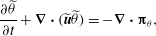 $$\begin{eqnarray}\frac{\partial \widetilde{{\it\theta}}}{\partial t}+\boldsymbol{{\rm\nabla}}\boldsymbol{\cdot }(\widetilde{\boldsymbol{u}}\widetilde{{\it\theta}})=-\boldsymbol{{\rm\nabla}}\boldsymbol{\cdot }\unicode[STIX]{x1D6D1}_{{\it\theta}},\end{eqnarray}$$
where
 $\unicode[STIX]{x1D6D1}_{{\it\theta}}=(\widetilde{\boldsymbol{u}{\it\theta}}-\widetilde{\boldsymbol{u}}\widetilde{{\it\theta}})$
is the SGS thermal flux.
The monodispersed air bubble mass concentration field is described by a continuous Eulerian scalar field
 $C_{b}(\boldsymbol{x},t)$
. The mass conservation of air bubbles yields an evolution equation for
 $C_{b}$
. Its filtered version is given by
 $$\begin{eqnarray}\displaystyle \frac{\partial \widetilde{C}_{b}}{\partial t}+\boldsymbol{{\rm\nabla}}\boldsymbol{\cdot }(\widetilde{\boldsymbol{v}}_{b}\widetilde{C}_{b})=-\boldsymbol{{\rm\nabla}}\boldsymbol{\cdot }\unicode[STIX]{x1D6D1}_{b}+q_{b},\end{eqnarray}$$
where
 $q_{b}$
is a source term (i.e., the mass release rate of bubbles per unit volume) representing release of the bubbles from an underwater blowout (which corresponds to the bubble diffuser in laboratory experiments),
 $\unicode[STIX]{x1D6D1}_{b}=(\widetilde{\boldsymbol{u}C_{b}}-\widetilde{\boldsymbol{u}}\widetilde{C}_{b})$
is the SGS air concentration flux, and
 $\boldsymbol{v}_{b}$
is the velocity of the air bubble phase. The resolved air bubble velocity is given by (Ferry & Balachandar Reference Ferry and Balachandar2001)
 $$\begin{eqnarray}\widetilde{\boldsymbol{v}}_{b}=\widetilde{\boldsymbol{u}}+w_{r}\boldsymbol{e}_{3}+\frac{w_{r}}{g}\frac{\text{D}\widetilde{\boldsymbol{u}}}{\text{D}t},\end{eqnarray}$$
where
 $w_{r}$
is the rise velocity (also known as slip or settling velocity) of bubbles, and
 $\text{D}\widetilde{\boldsymbol{u}}/\text{D}t=\partial \widetilde{\boldsymbol{u}}/\partial t+\widetilde{\boldsymbol{u}}\boldsymbol{\cdot }\boldsymbol{{\rm\nabla}}\widetilde{\boldsymbol{u}}$
. Included in (2.6) are the main effects acting on buoyant particles for the range of parameters typical of gas bubbles and oil droplets in the case of an underwater blowout: Stokes drag, gravitational force, added mass, and buoyancy. History force, Brownian motion, lift forces, SGS fluid stress force, and the Faxén corrections are neglected. Including these additional effects would severely increase computational cost and have a negligible impact on the results for the parameter ranges considered in this study (see e.g. Ferry & Balachandar Reference Ferry and Balachandar2001; Balachandar & Eaton Reference Balachandar and Eaton2010). A more detailed discussion of (2.6) is given in appendix A.
To track the behaviour of the entrained fluid, an additional passive scalar field
 $C_{dye}(\boldsymbol{x},t)$
is simulated to represent the mass concentration of dye in the laboratory experiments. The evolution of the dye concentration is governed by
 $$\begin{eqnarray}\displaystyle \frac{\partial \widetilde{C}_{dye}}{\partial t}+\boldsymbol{{\rm\nabla}}\boldsymbol{\cdot }(\widetilde{\boldsymbol{u}}\widetilde{C}_{dye})=-\boldsymbol{{\rm\nabla}}\boldsymbol{\cdot }\unicode[STIX]{x1D6D1}_{dye}+q_{dye},\end{eqnarray}$$
where
 $q_{dye}$
is a source term for the dye release and
 $\unicode[STIX]{x1D6D1}_{dye}=(\widetilde{\boldsymbol{u}C_{dye}}-\widetilde{\boldsymbol{u}}\widetilde{C}_{dye})$
is the SGS dye concentration flux. Note that the dye is considered as a tracer in both simulations and experiments, therefore it does not produce a buoyancy force in the momentum equation (2.2). Its transport velocity is simply the same as the fluid velocity
 $\widetilde{\boldsymbol{u}}$
, which differs from the bubble transport velocity
 $\widetilde{\boldsymbol{v}}_{b}$
in (2.5).
To close the equation system, the SGS stress tensor
 ${\bf\tau}^{d}$
is parameterized using the Lilly–Smagorinsky eddy-viscosity model (Smagorinsky Reference Smagorinsky1963; Lilly Reference Lilly1967),
 ${\it\tau}_{ij}^{d}=-2{\it\nu}_{{\it\tau}}\widetilde{\unicode[STIX]{x1D61A}}_{ij}=-2(c_{s}{\it\Delta})^{2}|\widetilde{\unicode[STIX]{x1D64E}}|\widetilde{\unicode[STIX]{x1D61A}}_{ij}$
, where
 $\widetilde{\unicode[STIX]{x1D61A}}_{ij}=(\partial \widetilde{u}_{i}/\partial x_{j}+\partial \widetilde{u}_{j}/\partial x_{i})/2$
is the resolved strain rate tensor,
 ${\it\nu}_{{\it\tau}}$
is the SGS eddy viscosity, and
 ${\it\Delta}$
is the grid (filter) scale. The Smagorinsky coefficient
 $c_{s}$
is determined dynamically during the simulation using the Lagrangian-averaged scale-dependent dynamic (LASD) SGS model, which is suitable for flows with strong spatial inhomogeneity (Bou-Zeid, Meneveau & Parlange Reference Bou-Zeid, Meneveau and Parlange2005). LES utilizing the LASD SGS model has been used in a number of prior studies of geophysical flows (e.g. Tseng, Meneveau & Parlange Reference Tseng, Meneveau and Parlange2006; Calaf, Meneveau & Meyers Reference Calaf, Meneveau and Meyers2010; Yang et al.
Reference Yang, Chamecki and Meneveau2014a
, Reference Yang, Chen, Chamecki and Meneveau2015; Yang, Meneveau & Shen Reference Yang, Meneveau and Shen2014b
,Reference Yang, Meneveau and Shen
c
). The current LES model also includes an eddy diffusivity closure for the SGS heat, air and dye fluxes (
 $\unicode[STIX]{x1D6D1}_{{\it\theta}}$
,
 $\unicode[STIX]{x1D6D1}_{b}$
and
 $\unicode[STIX]{x1D6D1}_{dye}$
, respectively). A simple but widely adopted approach is to prescribe the turbulent Prandtl number and Schmidt number
 $Pr_{{\it\tau}}=Sc_{{\it\tau}}=0.4$
. These values have been widely tested in prior studies (e.g. Antonopoulos-Domis Reference Antonopoulos-Domis1981; Moeng Reference Moeng1984; Mason Reference Mason1989; Sullivan, McWilliams & Moeng Reference Sullivan, Mcwilliams and Moeng1994; Kumar et al.
Reference Kumar, Kleissl, Meneveau and Parlange2006; Chamecki, Meneveau & Parlange Reference Chamecki, Meneveau and Parlange2009). The SGS fluxes are then parameterized as
 $\unicode[STIX]{x1D6D1}_{{\it\theta}}=-({\it\nu}_{{\it\tau}}/Pr_{{\it\tau}})\boldsymbol{{\rm\nabla}}\widetilde{{\it\theta}}$
,
 $\unicode[STIX]{x1D6D1}_{b}=-({\it\nu}_{{\it\tau}}/Sc_{{\it\tau}})\boldsymbol{{\rm\nabla}}\widetilde{C}_{b}$
, and
 $\unicode[STIX]{x1D6D1}_{dye}=-({\it\nu}_{{\it\tau}}/Sc_{{\it\tau}})\boldsymbol{{\rm\nabla}}\widetilde{C}_{dye}$
. With the SGS models for
 ${\bf\tau}^{d}$
,
 $\unicode[STIX]{x1D6D1}_{{\it\theta}}$
,
 $\unicode[STIX]{x1D6D1}_{b}$
and
 $\unicode[STIX]{x1D6D1}_{dye}$
, the governing equations (2.1)–(2.7) are closed and are solved numerically. Details of the numerical method are discussed in § 2.2.
2.2 Numerical method
The set of equations for velocity and temperature fields, (2.1), (2.2) and (2.4), are discretized by a pseudo-spectral method on a collocated grid in the horizontal directions and a second-order central difference method on a staggered grid in the vertical direction (Albertson & Parlange Reference Albertson and Parlange1999). Equation (2.2) is discretized in its rotational form, which provides good conservation of mass and kinetic energy (Orszag & Pao Reference Orszag and Pao1974; Ferziger & Perić Reference Ferziger and Perić2002). The velocity field is advanced in time by a fractional-step method. First, the momentum equation is integrated in time by the second-order Adams–Bashforth scheme. Then a Poisson equation for the pressure field is constructed by enforcing the divergence-free constraint (2.1) at the new time step. Finally, the velocity field from the time integration is projected to a divergence-free space with the correction from the pressure field. Similar to the momentum equation, the temperature equation (2.4) is integrated in time by the second-order Adams–Bashforth scheme.
Differently, the transport equations for concentration, (2.5) and (2.7), are discretized by a finite-volume algorithm. Because the velocity and concentration variables are defined on two different grid systems, a simple interpolation of the variables between the two grids would cause a non-divergence-free velocity field, unphysical oscillations in the concentration field, and even negative concentration, especially when simulating the transport of a highly inhomogeneous scalar field such as the buoyant plume studied in this work. To overcome this issue, Chamecki, Meneveau & Parlange (Reference Chamecki, Meneveau and Parlange2008) developed a hybrid method that uses a conservative interpolation scheme for exchanging information between the pseudo-spectral and finite-volume grids. The air bubble and dye concentration fields are then simulated using a finite-volume method with a bounded third-order upwind scheme for the advection term (Gaskell & Lau Reference Gaskell and Lau1988).
The hybrid LES turbulent flow and scalar field solver has also been tested extensively and applied to simulate particle and scalar dispersion in various geophysical flows in a number of prior LES studies (e.g. Chamecki et al. Reference Chamecki, Meneveau and Parlange2008, Reference Chamecki, Meneveau and Parlange2009; Chamecki & Meneveau Reference Chamecki and Meneveau2011; Pan, Chamecki & Isard Reference Pan, Chamecki and Isard2014, among many others). The basic framework of the current LES model has been tested, validated, and applied to oil spill dispersion in the upper ocean Langmuir turbulence by Yang et al. (Reference Yang, Chamecki and Meneveau2014a , Reference Yang, Chen, Chamecki and Meneveau2015). Similar evolution equations to those in (2.1)–(2.6) have been applied to simulate bubble plumes in stratified fluid before, for various conditions (see, for example, the review for laboratory-scale applications by Sokolichin, Eigenberger & Lapin (Reference Sokolichin, Eigenberger and Lapin2004) and the more recent paper by Fabregat et al. (Reference Fabregat, Dewar, Özgökmen, Poje and Wienders2015)). The simulation cases considered in this study fall well within the parameter ranges reported and justified in these previous studies.
3 Integral model for multiphase plume
High-fidelity three-dimensional computational fluid dynamics (CFD) models, such as large-eddy simulation and direct numerical simulation, can provide detailed instantaneous plume structures for studying the fundamental physics, with the price of high computational cost. Compared to the CFD models, the integral model significantly reduces computational cost and is thus more suitable for rapid predictions – for example, when rapid response to an underwater oil blowout is needed. Integral models usually approximate the lateral variations of the plume to be top hat or Gaussian, and model the integrated quantities on each lateral plane as a function of the height
 $z$
(i.e. the coordinate along the plume axis) (e.g. Morton et al.
Reference Morton, Taylor and Turner1956; Morton Reference Morton1962).
Taking the recent double-plume integral model (Crounse et al. Reference Crounse, Wannamaker and Adams2007; Socolofsky et al. Reference Socolofsky, Bhaumik and Seol2008) as an example, the behaviour of the inner and outer plumes are governed by conservation of mass in the inner and outer plumes (with the fluid density cancelled on both sides of the equation based on the Boussinesq approximation),
 $$\begin{eqnarray}\displaystyle & \displaystyle \frac{\text{d}Q_{i}}{\text{d}z}=E_{i}+E_{o}+E_{p}, & \displaystyle\end{eqnarray}$$
 $$\begin{eqnarray}\displaystyle & \displaystyle \frac{\text{d}Q_{o}}{\text{d}z}=E_{a}-E_{o}-E_{i}-E_{p}. & \displaystyle\end{eqnarray}$$
Here
 $Q_{i}$
and
 $Q_{o}$
are the vertical volume fluxes in the inner and outer plumes, defined respectively according to:
 $$\begin{eqnarray}\displaystyle & \displaystyle Q_{i}=\int _{0}^{b_{i}}\langle \overline{w}\rangle (r,z)\,2{\rm\pi}r\,\text{d}r, & \displaystyle\end{eqnarray}$$
 $$\begin{eqnarray}\displaystyle & \displaystyle Q_{o}=\int _{b_{i}}^{b_{o}}\langle \overline{w}\rangle (r,z)\,2{\rm\pi}r\,\text{d}r, & \displaystyle\end{eqnarray}$$
where
 $b_{i}$
and
 $b_{o}$
are the half-width of the inner and outer plumes, respectively;
 $\langle \overline{w}\rangle$
is the time- and angular-averaged vertical velocity;
 $E_{i}$
is the entrainment flux per unit depth from the outer plume or ambient fluid into the inner plume;
 $E_{o}$
is the entrainment flux per unit depth from the inner plume into the outer plume;
 $E_{p}$
is the peeling flux per unit depth;
 $E_{a}$
is the entrainment flux per unit depth from the ambient fluid into the outer plume. The signs of
 $E_{i}$
,
 $E_{o}$
and
 $E_{p}$
are defined with respect to the inner plume, i.e.
 $E_{i}\geqslant 0$
,
 $E_{o}\leqslant 0$
and
 $E_{p}\leqslant 0$
; the sign of
 $E_{a}$
is defined with respect to the outer plume, i.e.
 $E_{a}\geqslant 0$
. The structure of the mean plume is sketched in figure 1.
Schematic of the mean plume structure for the integral model. Several key entrainment and detrainment fluxes are indicated in the plot:
 $E_{i}$
, net entrainment flux per unit height into the inner plume from either the ambient fluid or the outer plume;
 $E_{o}$
, net detrainment flux per unit height from the inner plume into the outer plume;
 $E_{a}$
, net entrainment flux per unit height from the ambient fluid into the outer plume;
 $E_{p}$
, net peel flux per unit height from the top portion of the inner plume to the outer plume;
 $Q_{i}$
, upward volumetric flux of the entrained fluid in the inner plume;
 $Q_{o}$
, downward volumetric flux of the detrained fluid in the outer plume.

Also needed is the conservation of momentum flux. Assuming a top-hat velocity for the inner and outer plumes (i.e.
 $W_{i}$
and
 $W_{o}$
, respectively), the integrated momentum conservation can be written as
 $$\begin{eqnarray}\displaystyle & \displaystyle \frac{\text{d}(Q_{i}W_{i})}{\text{d}z}=\left(1-\frac{{\it\rho}_{b}}{{\it\rho}_{r}}\right)\frac{\langle \overline{C}_{b}\rangle _{i}}{{\it\rho}_{b}}g{\rm\pi}b_{i}^{2}+\left(1-\frac{\langle \overline{{\it\rho}}\rangle _{i}}{\langle \overline{{\it\rho}}\rangle _{h}}\right)g{\rm\pi}b_{i}^{2}+E_{i}W_{o}+E_{o}W_{i}+E_{p}W_{i},\qquad & \displaystyle\end{eqnarray}$$
 $$\begin{eqnarray}\displaystyle & \displaystyle \frac{\text{d}(Q_{o}W_{o})}{\text{d}z}=\left(1-\frac{\langle \overline{{\it\rho}}\rangle _{o}}{\langle \overline{{\it\rho}}\rangle _{h}}\right)g{\rm\pi}(b_{o}^{2}-b_{i}^{2})-E_{o}W_{i}-E_{i}W_{o}-E_{p}W_{i},\qquad & \displaystyle\end{eqnarray}$$
where the volume fluxes and top-hat plume velocities are related by
 $$\begin{eqnarray}\displaystyle & \displaystyle W_{i}(z)=\frac{Q_{i}}{{\rm\pi}b_{i}^{2}}, & \displaystyle\end{eqnarray}$$
 $$\begin{eqnarray}\displaystyle & \displaystyle W_{o}(z)=\frac{Q_{o}}{{\rm\pi}(b_{o}^{2}-b_{i}^{2})}. & \displaystyle\end{eqnarray}$$
In (3.5) and (3.6),
 $\langle \overline{C}_{b}\rangle _{i}$
is the time and planar average of the bubble mass concentration in the inner plume;
 $\langle \overline{{\it\rho}}\rangle _{i}$
is the time and planar average of the fluid density in the inner plume;
 $\langle \overline{{\it\rho}}\rangle _{o}$
is the time and planar average of the fluid density in the outer plume; and
 $\langle \overline{{\it\rho}}\rangle _{h}$
is the time and planar average of the fluid density over the entire horizontal plane. Equations (3.1), (3.2), (3.5) and (3.6) can be obtained by integrating the filtered Navier–Stokes equation over time and over the cross-plume planes (e.g. Buscaglia, Bombardelli & García Reference Buscaglia, Bombardelli and García2002).
Note that the integral model equations (3.1), (3.2), (3.5) and (3.6) are written in a planar average context. If the inner and outer plume velocity profiles are assumed to be top hat, as in (3.7) and (3.8), all the primary variables in the integral model are a function only of the depth
 $z$
. It is worth mentioning that the inner plume velocity profile can also be assumed to be Gaussian, which will make model equations more complicated (e.g. McDougall Reference McDougall1978; Milgram Reference Milgram1983). As shown by Davidson (Reference Davidson1986) for a condition with inner plume only, the additional physical information provided by a Gaussian formulation (e.g. radial variation in the plume cross-section) plays only a minor role when modelling mean plume behaviour. For the double-plume cases studied here, the inner and outer plume have complex interactions and cannot have a pure Gaussian form for their profiles. The top-hat profiles are the least complicated, and thus have been chosen in most of the previous studies for double plumes (e.g. Asaeda & Imberger Reference Asaeda and Imberger1993; Crounse et al.
Reference Crounse, Wannamaker and Adams2007; Socolofsky et al.
Reference Socolofsky, Bhaumik and Seol2008).
4 LES results of multiphase buoyant plumes
4.1 LES configuration
In this study, the large-eddy simulations use a rectangular prism domain with size
 $(L_{x},L_{y},H)=(0.76,0.76,0.9)~\text{m}$
to mimic a water tank in laboratory measurements (Seol et al.
Reference Seol, Bryant and Socolofsky2009). Note that the pseudo-spectral flow solver in the LES uses periodic boundary conditions in the horizontal directions. To limit the influence of the side boundaries and provide sufficient horizontal space for the intrusion layer to expand during the simulation period, in this study the LES domain is chosen to be twice as long and twice as wide as the experimental water tank (
 $L_{x}=L_{y}=0.38~\text{m}$
in Seol et al. (Reference Seol, Bryant and Socolofsky2009)). Test runs with a smaller domain of
 $(L_{x},L_{y},H)=(0.6,0.6,0.9)~\text{m}$
(not shown) yield results consistent with the cases reported in this paper, indicating the domain size chosen in this study is sufficient. The top boundary of the simulation domain is kept flat and stress-free. For the bottom boundary, we assume a flat surface on which a small friction drag is specified using the traditional equilibrium logarithmic wall model (as used in Bou-Zeid et al.
Reference Bou-Zeid, Meneveau and Parlange2005), with an imposed roughness length of 0.0001 m. The simulations use
 $N_{x}\times N_{y}\times N_{z}=150\times 150\times 257$
grid points for spatial discretization and a time step of
 ${\rm\Delta}t=0.001~\text{s}$
for time integration.
The air bubble concentration field is released from a localized source with a rate of
 $Q_{b}=0.09~\text{l min}^{-1}$
. The bubble air density is taken to be
 ${\it\rho}_{b}=1.4~\text{kg m}^{-3}$
. The air source is located at 0.8 m below the top boundary. By setting the origin of the vertical coordinate to be at the centre of the air source, the vertical domain ranges from
 $z=-0.1$
to
 $0.8~\text{m}$
. This gives a
 $0.1~\text{m}$
distance from the air source to the bottom of the simulation domain, similar to the experimental condition in which the air diffuser was placed some distance above the bottom of the water tank. The air source is smeared smoothly using a super Gaussian function over a finite cylindrical volume of
 $V_{s}={\rm\pi}b_{s}^{2}{\rm\Delta}z$
, with a source radius
 $b_{s}\approx 7~\text{mm}$
and a height
 ${\rm\Delta}z=3.5~\text{mm}$
(i.e. one vertical grid size).
The water in the simulation domain is initially quiescent and is linearly stratified from
 $z=-0.1~\text{m}$
(bottom) to
 $z=0.7~\text{m}$
with
 $\partial {\it\rho}/\partial z=-50~\text{kg m}^{-4}$
, corresponding to a buoyancy frequency of
 $N=\sqrt{-(g/{\it\rho}_{r})\partial {\it\rho}/\partial z}=0.7~\text{s}^{-1}$
. Similar to the experiment, the top
 $0.1~\text{m}$
of the simulation domain has a uniform water density of
 ${\it\rho}_{r}=1000~\text{kg m}^{-3}$
, mimicking the effect of the surface mixed layer in the ocean.
As shown by Socolofsky, Crounse & Adams (Reference Socolofsky, Crounse, Adams, Shen, Cheng, Wang and Teng2002) (also see Socolofsky & Adams Reference Socolofsky and Adams2005), the characteristics of a multiphase buoyant plume can be categorized based on the dimensionless bubble rise velocity
 $$\begin{eqnarray}U_{N}=w_{r}/(B_{s}N)^{1/4},\end{eqnarray}$$
where
 $B_{s}=gQ_{b}({\it\rho}_{r}-{\it\rho}_{b})/{\it\rho}_{r}=1.47\times 10^{-5}~\text{m}^{4}~\text{s}^{-3}$
is the kinematic buoyancy flux induced by the bubble source. In this study, we consider a baseline case matching the experiment reported in Seol et al. (Reference Seol, Bryant and Socolofsky2009), with
 $w_{r}=0.06~\text{m s}^{-1}$
, which corresponds to
 $U_{N}=1.06$
. We also consider three additional cases with
 $w_{r}=0.03$
, 0.12 and
 $0.20~\text{m s}^{-1}$
, corresponding to
 $U_{N}=0.53$
, 2.12 and 3.53. Based on the rise velocity, the four simulation cases are named WR3, WR6, WR12 and WR20. The key parameters for these four cases are summarized in table 1. Among them, case WR6 is the baseline case with available experimental data from Seol et al. (Reference Seol, Bryant and Socolofsky2009) for comparison.
Key parameters for the large-eddy simulation. For all cases, the source bubble volume flux is
 $Q_{b}=0.09~\text{l min}^{-1}$
, the source buoyancy flux is
 $B_{s}=gQ_{b}({\it\rho}_{r}-{\it\rho}_{b})/{\it\rho}_{r}=1.47\times 10^{-5}~\text{m}^{4}~\text{s}^{-3}$
, and
 $N=\sqrt{-(g/{\it\rho}_{r})\partial {\it\rho}/\partial z}=0.7~\text{s}^{-1}$
. In the table,
 $w_{r}$
and
 $U_{N}=w_{r}/(B_{s}N)^{1/4}$
are the dimensional and dimensionless bubble rise velocities, respectively;
 $d$
is the effective spherical diameter of the air bubble;
 $\overline{h}_{P}$
and
 $H_{P}=\overline{h}_{P}/(B_{s}/N^{3})^{1/4}$
are the dimensional and dimensionless plume peel heights, respectively;
 $\overline{h}_{T}$
and
 $H_{T}=\overline{h}_{T}/(B_{s}/N^{3})^{1/4}$
are the dimensional and dimensionless plume trap heights, respectively;
 $Q_{s}$
is the inner plume volume flux near the source;
 $M_{s}$
is the inner plume momentum flux near the source;
 $L_{j}=M_{s}^{3/4}/B_{s}^{1/2}$
is the jet length over which the initial source momentum flux is important (Fischer et al.
Reference Fischer, List, Koh, Imberger and Brooks1979);
 $L_{q}=Q_{s}/M_{s}^{1/2}$
is a characteristic length over which the initial volume flux is more significant than the entrained fluxes (Hunt, Cooper & Linden Reference Hunt, Cooper and Linden2001);
 $We={\it\rho}_{r}w_{r}^{2}d/{\it\sigma}$
is the Weber number;
 $Mo={\it\mu}_{f}^{4}g/({\it\sigma}^{3}{\it\rho}_{r})$
is the Morton number;
 ${\it\chi}$
is the estimated bubble aspect ratio;
 ${\it\rho}_{r}=1000~\text{kg m}^{-3}$
is the reference water density;
 ${\it\sigma}=7.25\times 10^{-2}\;\text{N}\;\text{m}^{-1}$
is the bubble surface tension; and
 ${\it\mu}_{f}=1.0\times 10^{-3}~\text{N s m}^{-2}$
is the dynamic viscosity of the water. In the table, the values for
 $d$
are determined based on the desired
 $w_{r}$
using the empirical parameterization reported in Zheng & Yapa (Reference Zheng and Yapa2000).

For each case, the simulation is performed for 100 s, corresponding to
 $10^{5}$
time steps. The bubble and dye concentration fields are released from
 $t=0~\text{s}$
. Starting from
 $t=40~\text{s}$
, 250 three-dimensional snapshots of the entire simulation domain are recorded for statistical analysis with an interval of
 $0.25~\text{s}$
(i.e. 250 time steps) between each snapshot. The data sampling frequency is chosen to be the same as that of the planar laser-induced fluorescence measurements reported in Seol et al. (Reference Seol, Bryant and Socolofsky2009).
In table 1,
 $Q_{s}$
and
 $M_{s}$
are the initial volume and momentum fluxes of the plume at the source, respectively. Their values are estimated from the time-averaged LES results for each case. Based on them, the characteristics of the plume source can be further quantified by two length scales,
 $L_{j}$
and
 $L_{q}$
. In particular, the jet length
 $L_{j}=M_{s}^{3/4}/B_{s}^{1/2}$
is a characteristic length over which the initial source momentum flux is important (i.e. the plume is more jet-like), and
 $L_{q}=Q_{s}/M_{s}^{1/2}$
is a characteristic length over which the initial volume flux is significant compared with that entrained by the inner plume (Fischer et al.
Reference Fischer, List, Koh, Imberger and Brooks1979; Hunt et al.
Reference Hunt, Cooper and Linden2001). For all the cases, both
 $L_{j}$
and
 $L_{q}$
are much smaller than other characteristic lengths (such as the domain height
 $H$
, the peel height
 $h_{P}$
and the trap height
 $h_{T}$
), indicating that initial plume properties are not essential for characterizing the plume dynamics considered in this study. This is as expected since the plume is driven by a localized source with no initial volume flux introduced (note that the volume flux at the source is very small, but not exactly zero, as the flow accelerates within the volume of the bubble source). The insignificance of the initial plume volume and momentum fluxes is also consistent with the dimensional analysis and laboratory measurements reported in Socolofsky et al. (Reference Socolofsky, Crounse, Adams, Shen, Cheng, Wang and Teng2002).
In the current LES model, bubble deformation and breakup are not considered. As visualized in the experiment in Seol et al. (Reference Seol, Bryant and Socolofsky2009), bubble deformation was insignificant for the plume condition in case WR6. The same condition is expected for all the LES cases considered in this study. To confirm this, here the aspect ratios
 ${\it\chi}$
of the air bubbles in the four LES cases are estimated using the empirical parameterization reported in Legendre, Zenit & Velez-Cordero (Reference Legendre, Zenit and Velez-Cordero2012),
 $$\begin{eqnarray}{\it\chi}=\frac{1}{1-{\textstyle \frac{9}{64}}We[K(Mo)\,We]^{-1}}.\end{eqnarray}$$
Here the Weber number and Morton number are defined as
 $$\begin{eqnarray}\displaystyle & \displaystyle We={\it\rho}_{r}w_{r}^{2}d/{\it\sigma}, & \displaystyle\end{eqnarray}$$
 $$\begin{eqnarray}\displaystyle & \displaystyle Mo={\it\mu}_{f}^{4}g/({\it\sigma}^{3}{\it\rho}_{r}), & \displaystyle\end{eqnarray}$$
respectively, where
 $d$
is the effective spherical diameter of the air bubble,
 ${\it\sigma}$
is the bubble surface tension, and
 ${\it\mu}_{f}$
is the dynamic viscosity of the water. In (4.2),
 $K(Mo)$
is a function of the Morton number only, and has a simple expression given by Legendre et al. (Reference Legendre, Zenit and Velez-Cordero2012)
 $$\begin{eqnarray}K(Mo)=0.2Mo^{1/10}.\end{eqnarray}$$
As listed in table 1, the estimated bubble aspect ratio
 ${\it\chi}$
is close to 1 for all the four LES cases reported in this study, indicating that bubble deformation is insignificant for the plume conditions considered here. Moreover, as pointed out by Asaeda & Imberger (Reference Asaeda and Imberger1993), for the laboratory-scale conditions considered in this study the water depth is limited so that bubble coalescence or expansion can also be neglected.
4.2 Instantaneous plume structures
Figure 2 shows a two-dimensional snapshot of the instantaneous plume from case WR6 taken at
 $t=90~\text{s}$
. The
 $(x,z)$
-plane across the centre of the plume source is plotted, with the contours of the resolved air bubble concentration
 $\widetilde{C}_{b}$
, dye concentration
 $\widetilde{C}_{dye}$
, vertical velocity
 $\widetilde{w}$
, and density
 $\widetilde{{\it\rho}}$
shown in 2(a–d), respectively. After being released from the source, the air bubbles rise along a vertical column (figure 2
a). Due to the much smaller bubble density
 ${\it\rho}_{b}$
compared to the reference water density
 ${\it\rho}_{r}$
, a positive buoyancy force per unit volume of
 $$\begin{eqnarray}F_{b}=({\it\rho}_{r}/{\it\rho}_{b}-1)\widetilde{C}_{b}g\end{eqnarray}$$
per unit volume is induced by the concentrated bubbles, which causes the ambient fluid to rise with the bubbles. As the plume rises, it also entrains ambient fluid from the side by the action of turbulent eddies. The rise of entrained fluid can be seen from the elevated dye concentration in figure 2(b) and the upward fluid velocity in the core of the plume in figure 2(c). The turbulent entrainment causes the plume to spread and decelerate. The rising velocity of the fluid in the plume reaches its maximum value at approximately
 $z=0.08~\text{m}$
and gradually decreases towards higher elevation (figure 2
c).
Instantaneous velocity and scalar fields for case WR6 at
 $t=90~\text{s}$
: (a) air concentration
 $\widetilde{C}_{b}$
(
 $\text{kg m}^{-3}$
); (b) dye concentration
 $\widetilde{C}_{dye}$
(
 $\text{kg m}^{-3}$
); (c) vertical velocity
 $\widetilde{w}$
(
 $\text{m s}^{-1}$
); and (d) density
 $\widetilde{{\it\rho}}$
(
 $\text{kg m}^{-3}$
). Here the
 $(x,z)$
-plane across the centre of the plume source is shown. The averaged peel and trap heights from the laboratory measurement (Seol et al.
Reference Seol, Bryant and Socolofsky2009) are indicated in (b) by the dashed and dash-dot lines, respectively.

Moreover, as entrained fluid is transported upwards, its density becomes higher than that of the local environment, producing a negative volumetric buoyancy force
 $$\begin{eqnarray}F_{i}=(\langle \widetilde{{\it\rho}}\rangle _{h}-\widetilde{{\it\rho}})g,\end{eqnarray}$$
where
 $\langle \widetilde{{\it\rho}}\rangle _{h}$
is the horizontally averaged fluid density as in (2.2). As shown in figure 2(d), the fluid entrained in the plume has a higher density than that of the ambient fluid, such that
 $F_{i}<0$
. Because the magnitude of the negative force
 $F_{i}$
keeps increasing as the entrained fluid rises, eventually the magnitude of
 $F_{i}$
exceeds
 $F_{b}$
and induces considerable resistance to the upward flow inside the plume.
Further up, the entrained fluid starts peeling off from the bubble column and forms an annular plume outside the inner plume with downward velocity, as shown in figure 2(c) for negative velocities outside the plume core in the region between 0.15 and 0.35 m height. When the detrained fluid falls down to its equilibrium height, it moves outwards horizontally, forming a lateral intrusion layer (Asaeda & Imberger Reference Asaeda and Imberger1993; Socolofsky & Adams Reference Socolofsky and Adams2003, Reference Socolofsky and Adams2005). Meanwhile, the outward radial velocity in the peeling zone causes a broadening of the bubble column core. As shown in figure 2(a), the bubble column is narrow near the bottom of the plume, and becomes wider near and above the peeling region (between 0.3 and 0.5 m height). This broadening effect also reduces the local air bubble concentration inside the inner plume, which results in a weaker bubble-induced buoyancy force and a weak and unstable subsequent double-plume structure above the first peeling region. These trends observed in the current LES agree with the experimental results of Socolofsky et al. (Reference Socolofsky, Crounse, Adams, Shen, Cheng, Wang and Teng2002), Socolofsky & Adams (Reference Socolofsky and Adams2005) and Seol et al. (Reference Seol, Bryant and Socolofsky2009).
The instantaneous plume structure is unsteady because of the turbulent counter flow motions in the inner and outer plumes. The inner plume wanders around its axis, and the peeling and outer downward flows show intermittent behaviour that correlates with the wandering motion of the inner plume (figure 2
c). To quantify the oscillation of the plume, the instantaneous peel and trap heights are calculated based on the dye concentration on the
 $(x,z)$
-plane across the plume centre (i.e. the plane shown in figure 2), as was also done in Seol et al. (Reference Seol, Bryant and Socolofsky2009). Following Seol et al. (Reference Seol, Bryant and Socolofsky2009), 5 % of the maximum dye concentration is used as the cutoff threshold to distinguish the plume structure from the background fluid. The instantaneous peel height
 $h_{P}$
is then defined as the height of the highest point of the truncated dye concentration field. Different from
 $h_{P}$
, the instantaneous trap (or intrusion) height of the detrained fluid,
 $h_{T}$
, is evaluated based on the height of the centre of mass of the dye associated with trapping (by excluding the averaged inner plume which will be defined in § 4.3). Seol et al. (Reference Seol, Bryant and Socolofsky2009) used a similar approach to evaluate
 $h_{T}$
from the LIF data, except that they first converted the LIF images into black and white images (based on the same 5 % threshold when evaluating
 $h_{P}$
) and then calculated the centre of mass of the latter. The difference between these two
 $h_{T}$
evaluation approaches is found to be negligible (i.e. less than 3 %) when applied to analyse the LES data in this study.
Figure 3 shows the instantaneous peel height
 $h_{P}$
and trap height
 $h_{T}$
for case WR6, as a function of time. Some oscillations can be observed for both
 $h_{P}$
and
 $h_{T}$
. The curve for
 $h_{T}$
is considerably smoother than
 $h_{P}$
because of the averaging effect associated with the centre-of-mass calculation. The time-averaged values for the LES results are
 $\overline{h}_{P}=330~\text{mm}$
and
 $\overline{h}_{T}=170~\text{mm}$
. These values agree reasonably well with the experimental data reported in Seol et al. (Reference Seol, Bryant and Socolofsky2009) (see their figure 4), which yields a steady-state average of
 $\overline{h}_{P}=311~\text{mm}$
and
 $\overline{h}_{T}=146~\text{mm}$
(averaged based on experimental record from
 $t=30$
to 75 s). The experimental results of
 $\overline{h}_{P}$
and
 $\overline{h}_{T}$
are also indicated in figures 2(b) and 3. For case WR6, the
 $\overline{h}_{T}$
value from the LES is approximately 16 % larger than that from Seol et al. (Reference Seol, Bryant and Socolofsky2009), which may be due partly to the simplification of the small-scale bubble dynamics in the LES, but may also be due to the uncertainties in the experiment. The bubble rise velocity could be affected by bubble–bubble interactions (drafting) which has been neglected in determining the rise velocity from the bubble diameter in the experiments (Seol et al.
Reference Seol, Bryant and Socolofsky2009) and also is not included in the LES.
Time history of the instantaneous peel height (
 $h_{P}$
) and trap height (
 $h_{T}$
) from LES case WR6 are shown as solid lines. The corresponding mean values from the LES (dotted lines) and from the experimental data of Seol et al. (Reference Seol, Bryant and Socolofsky2009) (dashed lines) are also shown.

Moreover, spectral analysis of the LES results shows that the spectra of
 $h_{P}$
and
 $h_{T}$
have the peak frequency at approximately 0.09 Hz (not shown), which also agrees well with the experimental result in Seol et al. (Reference Seol, Bryant and Socolofsky2009) (see their figure 4). As pointed out by Seol et al. (Reference Seol, Bryant and Socolofsky2009), this periodic oscillation of peeling/trapping process is generated by coherent structures in the plume itself, which is different from the tank-scale recirculation cells or the buoyancy frequency induced by the stratification. As shown in figure 2, the downward flow velocity in the outer plume from the peel height to the trap height is
 ${\sim}0.03~\text{m}$
on average, and the distance between peel and trap heights is
 ${\sim}0.16~\text{m}$
, so that the time duration for the peeled fluid to fall is
 ${\sim}5.3~\text{s}$
. Note that this time duration corresponds to half of the oscillation period, since the downward plume will then rise back and oscillate around the trap height. Therefore, the estimated oscillation frequency is expected to be
 ${\sim}0.1~\text{Hz}$
, very close to the 0.09 Hz obtained by spectral analysis.
4.3 Time- and angular-averaged plume structure
Although the instantaneous plume structure is highly turbulent, the time- and angular-averaged plume obtained from the available data is smooth, as shown in figure 4. To obtain the mean plume structure in figure 4, the original instantaneous snapshots on the Cartesian coordinate
 $(x,y,z)$
are first interpolated to a cylindrical coordinate
 $(r,{\it\varphi},z)$
, and then averaged both in time (denoted by
 $\overline{f}$
) and along the angular (
 ${\it\varphi}$
) direction (denoted by
 $\langle f\rangle$
). Based on the averaged vertical velocity
 $\langle \overline{\widetilde{w}}\rangle$
, the edges of the inner and outer plumes can been estimated. In particular, the outer edge of the inner plume (the dash-dot line in figure 4) is identified by the contour line of
 $\langle \overline{\widetilde{w}}\rangle =0.002~\text{m s}^{-1}$
, and the outer edge of the outer plume (the dash-dot-dot line in figure 4) is identified based on
 $\langle \overline{\widetilde{w}}\rangle =-0.002~\text{m s}^{-1}$
. Here a small but non-zero value is chosen as the threshold for
 $\langle \overline{\widetilde{w}}\rangle$
to ensure a smooth and reliable estimation of the plume width. Because there is no cross-plume current, the inner and outer plumes are statistically axisymmetric, resulting in a pancake shape for the lateral intrusion layer, as indicated by the contour line of the 1 % maximum averaged dye concentration (figure 4
a). At the bottom of the plume, where no outer plume is present (i.e.
 $z\lesssim 0.1~\text{m}$
), the core of the inner plume expands linearly with a spreading ratio of approximately 0.11 (indicated by the white dashed line in figure 4
a), the same as the spreading ratio measured in Seol et al. (Reference Seol, Bryant and Socolofsky2009).
Time- and angular-averaged buoyant plume for case WR6: (a) dye concentration
 $\langle \overline{\widetilde{C}}_{dye}\rangle$
(
 $\text{kg m}^{-3}$
); (b) vertical velocity
 $\langle \overline{\widetilde{w}}\rangle$
(
 $\text{m s}^{-1}$
); and (c) radial velocity
 $\langle \overline{\widetilde{u}}_{r}\rangle$
(
 $\text{m s}^{-1}$
). In (a–c), the thin lines indicate streamlines of the mean flow; the black dash-dot line indicates the interface between the inner and outer plumes; the black dash-dot-dot line indicates the outer edge of the downdraught in the outer plume; and the thick red solid line corresponds to
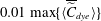 $0.01\max \{\langle \overline{\widetilde{C}}_{dye}\rangle \}$
. In (a), the white dashed line indicates a linear expansion with a spreading ratio of 0.11 for the bottom part of the plume.

Figure 4 also displays the averaged velocity field, which can help identify the path followed by the entrained fluid. Following the streamlines, first the ambient fluid is entrained laterally into the lower portion of the inner plume (at
 $z\lesssim 0.1~\text{m}$
), which is also indicated by the negative contours of the mean radial velocity
 $\langle \overline{\widetilde{u}}_{r}\rangle$
(figure 4
c). Then the streamlines turn upwards (i.e.
 $\langle \overline{\widetilde{w}}\rangle >0$
) to become aligned with the core of the inner plume. The magnitude of
 $\langle \overline{\widetilde{w}}\rangle$
increases with
 $z$
and reaches its peak at approximately
 $z=0.08~\text{m}$
, and then decreases gradually until approximately
 $z=0.25~\text{m}$
(figure 4
b), where its magnitude starts decreasing rapidly due to peeling. While the fluid in the centre still rises vertically, the mean streamlines near the edge of the inner plume turn outwards in the peeling region (
 $0.02~\text{m}\lesssim r\lesssim 0.03~\text{m}$
,
 $0.2~\text{m}\lesssim z\lesssim 0.3~\text{m}$
), where
 $\langle \overline{\widetilde{u}}_{r}\rangle$
is large (figure 4
c). The detrained fluid forms an annular outer plume, where the mean streamlines turn downwards. This outer plume descends and slightly overshoots at the lowest point of its trajectory, then rises back to the equilibrium trap height. Near the bottom of the downward outer plume, the mean streamlines turn to be horizontal again, and the detrained fluid migrates to form the lateral intrusion layer. In the intrusion layer, the mean radial velocity
 $\langle \overline{\widetilde{u}}_{r}\rangle$
is maximum in the vicinity of the outer plume, and decreases gradually when
 $r$
increases, because of the conservation of radial momentum flux.
4.4 Effect of bubble rise velocity on plume structure
The inner/outer double-plume structure makes it a challenging task to characterize the multiphase buoyant plume in a stratified environment. Previous laboratory observations (e.g. Asaeda & Imberger Reference Asaeda and Imberger1993; Socolofsky Reference Socolofsky2001; Socolofsky et al.
Reference Socolofsky, Crounse, Adams, Shen, Cheng, Wang and Teng2002) showed that the plume characteristics are controlled mainly by three parameters, i.e.
 $N$
,
 $B_{s}$
and
 $w_{r}$
. In particular, the buoyancy frequency
 $N$
represents the strength of the stratification: the larger
 $N$
, the stronger the ambient stratification, with a concomitant increase in difficulty to lift the entrained fluid. The kinematic buoyancy flux
 $B_{s}$
represents the capability for the bubble plume to entrain and lift the ambient fluid. The bubble rise (slip) velocity
 $w_{r}$
helps the bubbles to overcome the broadening effect of the peeling process and keep concentrated within the core of the inner plume (see the discussion in § 4.2), playing a key role in the formation of subsequent double-plume structures. The rise velocity also affects the magnitude of bubble concentrations in the inner plume, with higher
 $w_{r}$
causing lower bubble concentrations.
Instantaneous (a,c,e) air concentration
 $\widetilde{C}_{b}$
and (b,d,f) dye concentration
 $\widetilde{C}_{dye}$
(units in
 $\text{kg m}^{-3}$
at
 $t=90$
s) for various LES cases: (a,b) case WR3, (c,d) case WR12 and (e,f) case WR20.

Combining the three parameters, Socolofsky et al. (Reference Socolofsky, Crounse, Adams, Shen, Cheng, Wang and Teng2002) proposed a dimensionless parameter for characterizing the plume structure, the dimensionless bubble rise velocity
 $U_{N}=w_{r}/(B_{s}N)^{1/4}$
(also see § 4.1). As discussed in § 4.1, in this study the values of
 $B_{s}$
and
 $N$
are fixed to match the laboratory conditions of Seol et al. (Reference Seol, Bryant and Socolofsky2009), and four different values are considered for the rise velocity
 $w_{r}$
, corresponding to four
 $U_{N}$
, i.e. 0.53, 1.06, 2.12 and 3.53 (cases WR3, WR6, WR12 and WR20 in table 1, respectively). The laboratory observations by Socolofsky (Reference Socolofsky2001) (also see Socolofsky & Adams Reference Socolofsky and Adams2005) showed that, as
 $U_{N}$
increases, the plume transitions from having a more distinct peel/trap structure to having more frequent and unstable ones, as was first observed by Asaeda & Imberger (Reference Asaeda and Imberger1993). The current LES results are found to support the plume classification by Socolofsky et al. (Reference Socolofsky, Crounse, Adams, Shen, Cheng, Wang and Teng2002). Figure 5 shows the snapshots of the instantaneous plume for cases WR3, WR12 and WR20 (cf. case WR6 in figure 2). In cases WR3 and WR6, the air bubbles concentrate in a narrow and stable column until the first peeling zone (
 $z\approx 0.3~\text{m}$
), resulting in a distinct peel zone and intrusion layer. After the first peeling event, the bubble plume becomes broader and unstable (figures 2
a and 5
a), resulting in less well-defined peels/intrusions after that (figures 2
b and 5
b) (for additional discussions, also see Socolofsky & Adams Reference Socolofsky and Adams2005).
To help interpret the effect of the bubble rise velocity on the plume structure, here the rates of work of the buoyancy forces acting on the entrained fluid in the inner plume are calculated and compared for the four LES cases. Figure 6 shows the profiles of the averaged rate of work per unit mass by the bubble-induced positive buoyancy force,
 $$\begin{eqnarray}B_{b}(z)=\left(1-\frac{{\it\rho}_{b}}{{\it\rho}_{r}}\right)\frac{\langle \overline{C}_{b}\rangle _{i}}{{\it\rho}_{b}}g{\rm\pi}b_{i}^{2}W_{i},\end{eqnarray}$$
and that by the stratification-induced negative buoyancy force,
 $$\begin{eqnarray}B_{i}(z)=\left(1-\frac{\langle \overline{{\it\rho}}\rangle _{i}}{\langle \overline{{\it\rho}}\rangle _{h}}\right)g{\rm\pi}b_{i}^{2}W_{i}.\end{eqnarray}$$
The physical meanings of the symbols in (4.8) and (4.9) have been defined in § 3. As
 $U_{N}$
increases (due to the increase of
 $w_{r}$
), the larger
 $w_{r}$
gives the bubbles less time to form high concentration (per unit vertical height and integrated within the inner plume). This results in a smaller
 $\langle \overline{C}_{b}\rangle _{i}$
, and thus a smaller
 $B_{b}$
for cases with larger
 $U_{N}$
, as shown in figure 6 (thin lines). Meanwhile, increasing
 $U_{N}$
also causes bubbles to be distributed over a narrower core width. The combined effect of smaller
 $B_{b}$
and narrower core results in less efficient pumping of denser entrained water vertically upwards, which in turn results in weaker peeling, as shown in figure 6 (thick lines), and hence weaker intrusion flows. Associated with the decrease in peeling intensity, the fraction of inner plume fluid that peels decreases monotonically with increasing
 $U_{N}$
, and a larger fraction of entrained denser fluid can enter the subsequent plume above the first peeling region. In particular, in cases WR12 and WR20, a considerable fraction of the very dense fluid from the bottom escapes the first peel and goes into the second plume, causing it to peel and trap frequently, which continues on up the plume. More discussions for the variation of the peeling fraction are given in § 5.2.
Profiles of the averaged rates of work by the buoyancy forces acting on the entrained fluid for various LES cases: — ⋅ ⋅ —, WR3; ——, WR6; – – –, WR12; and — ⋅ —, WR20. The thin lines with positive values are for
 $B_{b}$
, and the thick lines with negative values are for
 $B_{i}$
.

The instantaneous bubble and dye concentrations obtained by the current LES are consistent with the prior laboratory measurements (e.g. Socolofsky Reference Socolofsky2001; Socolofsky et al.
Reference Socolofsky, Crounse, Adams, Shen, Cheng, Wang and Teng2002; Socolofsky & Adams Reference Socolofsky and Adams2005). Moreover, the LES results show that in cases WR3 and WR6 the bubbles have temporarily detrained from the inner plume as they passed through the peeling/intrusion region, as indicated by the thin filaments of the air concentration contours near the edge of the inner plume at approximately
 $z=0.25~\text{m}$
(figures 2
a and 5
a); conversely, in cases WR12 and WR20 the air bubble plume remain relatively unaffected (figures 5
c and 5
e). This is consistent with the experimental observation in Socolofsky & Adams (Reference Socolofsky and Adams2005), where bubbles only began to detrain for
 $U_{N}\lesssim 1{-}1.5$
. Meanwhile, it appears that in none of the four LES cases did air bubbles enter the intrusion, which is consistent with the recent observations of Chan, Chow & Adams (Reference Chan, Chow and Adams2015), who suggested that bubbles (or particles) would only begin to enter the intrusion layer when
 $U_{N}\lesssim 0.2{-}0.4$
.
Time-averaged non-dimensional trap height
 $H_{T}=\overline{h}_{T}/(B_{s}/N^{3})^{1/4}$
as a function of the non-dimensional bubble rise velocity
 $U_{N}=w_{r}/(B_{s}N)^{1/4}$
. Results from the current LES are denoted by ▴. The data from various laboratory experiments are plotted for comparison: ○, Asaeda & Imberger (Reference Asaeda and Imberger1993); ▹, Lemckert & Imberger (Reference Lemckert and Imberger1993); ▿, Reingold (Reference Reingold1994); ♢, Socolofsky (Reference Socolofsky2001); ▫, Socolofsky & Adams (Reference Socolofsky and Adams2005); ▵, Seol et al. (Reference Seol, Bryant and Socolofsky2009). The integral plume model calculations by Crounse et al. (Reference Crounse, Wannamaker and Adams2007) are denoted by ——. The data from Reingold (Reference Reingold1994) were for sediments, while data from other experiments were for air bubbles.

Based on these instantaneous snapshots, further statistical analysis can be done in a way similar to the analysis reported in §§ 4.2 and 4.3. Figure 7 shows the dependence of the averaged dimensionless trap height
 $H_{T}=\overline{h}_{T}/(B_{s}/N^{3})^{1/4}$
on the dimensionless rise velocity
 $U_{N}$
:
 $H_{T}$
decreases monotonically as
 $U_{N}$
increases. Prior experimental data as well as a one-dimensional integral model calculation are also plotted for comparison. Despite the scatter in the experimental data, the current LES results fall within the range of the experimental data, and show consistent trends. The LES results also show good agreement with the integral model calculations by Crounse et al. (Reference Crounse, Wannamaker and Adams2007). Figure 8 shows the dependence of the averaged dimensionless peel height
 $H_{P}=\overline{h}_{P}/(B_{s}/N^{3})^{1/4}$
on
 $U_{N}$
. Fewer experimental datasets are available for
 $H_{P}$
than for
 $H_{T}$
. LES results predict somewhat smaller values for
 $H_{P}$
compared to the reported experimental data. Nevertheless, both LES and the experimental results indicate a peak value for
 $H_{P}$
in the moderate
 $U_{N}$
regime (i.e.
 $1.5\lesssim U_{N}\lesssim 2.4$
). The difference between the LES results and the experimental data are partly due to the relatively large uncertainty involved in evaluating
 $\overline{h}_{P}$
. As discussed in § 4.2,
 $\overline{h}_{P}$
is obtained by averaging the instantaneous peel height
 $h_{P}$
, which is noisy (see, for example, figure 3) because it is determined by the highest point on the plume edge in each instantaneous snapshot. For the laboratory data of Socolofsky & Adams (Reference Socolofsky and Adams2005) in figure 8,
 $H_{P}$
was evaluated by finding the location of the minimum dye concentration in the tank above the first intrusion after bubbling had stopped and all internal motion had died down; this point may be closer to the location of peak entrainment in the secondary plume structure above the peel zone, and thus is somewhat higher than the
 $H_{P}$
values evaluated based on the LES data. Note that for
 $H_{P}$
the current LES shows better agreement with more recent laboratory measurements (Seol et al.
Reference Seol, Bryant and Socolofsky2009), which used a similar way to calculate
 $H_{P}$
as in the current LES study.
Time-averaged non-dimensional peel hight
 $H_{P}=\overline{h}_{P}/(B_{s}/N^{3})^{1/4}$
as a function of the non-dimensional bubble rise velocity
 $U_{N}=w_{r}/(B_{s}N)^{1/4}$
.

It should also be mentioned that, for different experimental datasets, different sampling durations may be used for calculating the mean peel and trap heights. The estimated mean values are not expected to be sensitive to the averaging duration when the data are sampled in the steady-state range (i.e. when the instantaneous peel and trap heights have stabilized and oscillate around their mean values, see, for example, figure 3). Taking the baseline case WR6 as an example, the averaged peel and trap heights for five different averaging time intervals (i.e.
 $[30,75]~\text{s}$
,
 $[40,75]~\text{s}$
,
 $[50,75]~\text{s}$
,
 $[60,75]~\text{s}$
, and
 $[30,70]~\text{s}$
) show a relative difference of approximately 0.5 % or less, for both the current LES result and the experimental data from Seol et al. (Reference Seol, Bryant and Socolofsky2009).
Time- and angular-averaged (a,d,g) dye concentration
 $\langle \overline{\widetilde{C}}_{dye}\rangle$
(
 $\text{kg m}^{-3}$
), (b,e,h) vertical velocity
 $\langle \overline{\widetilde{w}}\rangle$
(
 $\text{m s}^{-1}$
), and (c,f,i) radial velocity
 $\langle \overline{\widetilde{u}}_{r}\rangle$
(
 $\text{m s}^{-1}$
) for various LES cases: (a–c) case WR3, (d–f) case WR12, and (g–i) case WR20. In (a–i), the thin lines indicate streamlines; the black dash-dot line indicates the interface between the inner and outer plumes; the black dash-dot-dot line indicates the outer edge of the downward flow in the outer plume; and the thick red solid lines correspond to
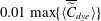 $0.01\max \{\langle \overline{\widetilde{C}}_{dye}\rangle \}$
.

Figure 9 shows the time- and angular-averaged plumes for cases WR3, WR12 and WR20. The averaged plume for case WR3 is similar to case WR6. In particular, the vertical velocity
 $\langle \overline{\widetilde{w}}\rangle$
in the inner plume reduces to very small values at approximately
 $z=0.3~\text{m}$
due to the significant peeling process (see figure 9
a–c). As a consequence of the strong peeling process, the radial velocity
 $\langle \overline{\widetilde{u}}_{r}\rangle$
is also significant both in the peeling zone and in the lateral intrusion layer, resulting in an extended intrusion layer.
As the dimensionless rise velocity
 $U_{N}$
increases, the inner core for the entrained fluid becomes narrower and nearly straight (see figures 9
d–f and 9
g–i) due to the narrower and more stable bubble column. The intensity of the first peeling event also decreases as
 $U_{N}$
increases, resulting in a continuously rising inner plume in cases WR12 and WR20 (note that in cases WR3 and WR6 the rising plume is interrupted after the first peeling at
 $z\approx 0.32~\text{m}$
in figure 4
b and figure 9
e). The weaker peeling events also result in a weaker radial velocity for the lateral intrusion layer to expand in cases WR12 and WR20 (figures 9
f and 9
i).
5 Integral properties of the plume
The time- and angular-averaged LES results exhibit a smooth and well-organized mean plume structure, suggesting that descriptions based on simpler models – for example, on integral quantities – should be possible. In this section, the concept of integral plume model and the associated flux parameterizations are tested a priori using the LES data.
5.1 Measurements and parameterization of the entrainment fluxes
In typical integral model calculations, the mass conservation (3.1) and (3.2) as well as the momentum conservation (3.5) and (3.6) are solved together, with
 $W_{i}$
,
 $W_{o}$
,
 $b_{i}$
and
 $b_{o}$
being the primary unknowns. The entrainment fluxes are unknown and require parameterizations based on the primary unknowns to close the model equations. Understanding the characteristics of these fluxes is crucial for developing accurate parameterizations that represent the essential physics. The LES provides high-fidelity temporal and spatial information of the plume structure, which can be used to evaluate the entrainment fluxes. Here the analysis focuses on the balances of mass and momentum fluxes across the inner/outer plume interface.
At the inner/outer plume interface
 $r=b_{i}$
, the three relevant entrainment fluxes (i.e.
 $E_{i}$
,
 $E_{o}$
and
 $E_{p}$
) are combined to form the net radial volume (
 $E_{net}$
) and momentum (
 $M_{net}$
) fluxes across the plume interface at each height according to
 $$\begin{eqnarray}\displaystyle & \displaystyle E_{i}(z)+E_{o}(z)+E_{p}(z)=E_{net}(z)=-2{\rm\pi}b_{i}\langle \overline{u}_{r}\rangle |_{r=b_{i}}, & \displaystyle\end{eqnarray}$$
 $$\begin{eqnarray}\displaystyle E_{i}(z)W_{o}(z)+[E_{o}(z)+E_{p}(z)]W_{i}(z) & = & \displaystyle M_{net}(z)=-2{\rm\pi}b_{i}\langle \overline{u_{r}w}\rangle |_{r=b_{i}}\nonumber\\ \displaystyle & = & \displaystyle -2{\rm\pi}b_{i}(\langle \overline{u}_{r}\rangle \langle \overline{w}\rangle +\langle \overline{u_{r}^{\prime }w^{\prime }}\rangle )|_{r=b_{i}},\end{eqnarray}$$
where
 $\langle \overline{u}_{r}\rangle$
denotes the time and angular average of the radial velocity. The peeling flux is defined as the net flux whenever it is negative:
 $$\begin{eqnarray}E_{p}(z)=E_{net}(z)\{1-H[E_{net}(z)]\},\end{eqnarray}$$
where
 $H$
is the Heaviside step function:
 $H(x)=1$
if
 $x>0$
and 0 otherwise. Solving (5.1) and (5.2) for
 $E_{i}$
and
 $E_{o}$
to express them in terms of the measurable quantities
 $E_{net}$
,
 $M_{net}$
,
 $W_{i}$
and
 $W_{o}$
gives
 $$\begin{eqnarray}\displaystyle & \displaystyle E_{i}=\frac{E_{net}W_{i}-M_{net}}{W_{i}-W_{o}}, & \displaystyle\end{eqnarray}$$
 $$\begin{eqnarray}\displaystyle & \displaystyle E_{o}=\frac{M_{net}-E_{net}W_{o}}{W_{i}-W_{o}}-E_{p}. & \displaystyle\end{eqnarray}$$
When experimental data or high-fidelity simulation results are available,
 $E_{net}$
and
 $M_{net}$
can be calculated based on the right-hand sides of (5.1) and (5.2), respectively. In the case of LES,
 $u_{r}$
and
 $w$
can be replaced by the corresponding LES resolved values,
 $\widetilde{u}_{r}$
and
 $\widetilde{w}$
, respectively, considering that most of the energy-significant fluid motions are resolved by LES. The values of
 $b_{i}$
and
 $b_{o}$
are determined based on the contours of
 $\langle \overline{\widetilde{w}}\rangle$
(see the dash-dot and dash-dot-dot lines shown in figures 4 and 9, as well as the related discussion in § 4.3).
Within the context of an integral model, where resolved data are not available, entrainment fluxes are typically parameterized as functions of
 $W_{i}$
,
 $W_{o}$
,
 $b_{i}$
and
 $b_{o}$
(e.g. Asaeda & Imberger Reference Asaeda and Imberger1993; Crounse et al.
Reference Crounse, Wannamaker and Adams2007; Socolofsky et al.
Reference Socolofsky, Bhaumik and Seol2008). These are the primary model variables when solving the integral model (3.1), (3.2), (3.5), (3.6). Specifically, the closures are written as:
 $$\begin{eqnarray}\displaystyle & \displaystyle E_{i}=2{\rm\pi}b_{i}{\it\alpha}_{i}(W_{i}-W_{o}), & \displaystyle\end{eqnarray}$$
 $$\begin{eqnarray}\displaystyle & \displaystyle E_{o}=2{\rm\pi}b_{i}{\it\alpha}_{o}W_{o}, & \displaystyle\end{eqnarray}$$
 $$\begin{eqnarray}\displaystyle & \displaystyle E_{a}=-2{\rm\pi}b_{o}{\it\alpha}_{a}W_{o}, & \displaystyle\end{eqnarray}$$
where
 ${\it\alpha}_{i}$
and
 ${\it\alpha}_{o}$
are dimensionless empirical transport efficiencies. A similar entrainment hypothesis has been used for modelling bubble plumes in non-stratified surroundings (e.g. Morton Reference Morton1962; Milgram Reference Milgram1983). The model coefficients
 ${\it\alpha}_{i}$
,
 ${\it\alpha}_{o}$
and
 ${\it\alpha}_{a}$
need to be prescribed a priori, and they can be estimated based on experimental data (e.g. Crounse et al.
Reference Crounse, Wannamaker and Adams2007; Socolofsky et al.
Reference Socolofsky, Bhaumik and Seol2008) or based on high-fidelity numerical simulations. In practice, the coefficient
 ${\it\alpha}_{a}$
is often assumed to equal to
 ${\it\alpha}_{o}$
. We remark that the closures (5.6)–(5.8) are for plumes in an ambient fluid or in a weak cross-stream. For conditions with strong cross-streams, the plume will incline towards the downstream direction, and additional effects such as the cross-stream velocity projected along the plume direction and the entrainment induced by the cross-stream have to be taken into account (Davidson Reference Davidson1986; Teixeira & Miranda Reference Teixeira and Miranda1997).
Vertical profiles of various statistics for interaction between inner and outer plumes for cases WR6 (square symbols and solid lines), WR12 (diamond symbols and dashed lines), and WR20 (circle symbols and dash-dot lines): (a) net volume fluxes
 $E_{net}$
; (b) net momentum fluxes
 $M_{net}$
; (c) averaged vertical velocities for inner (
 $W_{i}$
) and outer (
 $W_{o}$
) plumes; and (d) entrainment fluxes from outer to inner plume,
 $E_{i}$
; (f) detrainment fluxes from inner to outer plume,
 $E_{o}$
; and (e) peel fluxes from inner to outer plume,
 $E_{p}$
.

Here the LES data are used to evaluate the entrainment coefficients
 ${\it\alpha}_{i}$
and
 ${\it\alpha}_{o}$
. First
 $E_{net}$
and
 $M_{net}$
are calculated using LES data based on the right-hand side of (5.1) and (5.2), respectively. Then the peeling flux
 $E_{p}$
is calculated based on (5.3). Finally,
 $E_{i}$
and
 $E_{o}$
are obtained from (5.4) and (5.5). Figure 10 shows the profiles of
 $E_{net}$
,
 $M_{net}$
,
 $W_{i}$
,
 $W_{o}$
,
 $E_{i}$
,
 $E_{o}$
and
 $E_{p}$
calculated from the LES data. Then the coefficients for the entrainment models can be obtained based on (5.6) and (5.7), which can be rewritten as
 $$\begin{eqnarray}\displaystyle & \displaystyle {\it\alpha}_{i}=\frac{E_{i}}{2{\rm\pi}b_{i}(W_{i}-W_{o})}, & \displaystyle\end{eqnarray}$$
 $$\begin{eqnarray}\displaystyle & \displaystyle {\it\alpha}_{o}=\frac{E_{o}}{2{\rm\pi}b_{i}W_{o}}. & \displaystyle\end{eqnarray}$$
Figure 11 shows the vertical profiles of the directly measured entrainment coefficients
 ${\it\alpha}_{i}$
and
 ${\it\alpha}_{o}$
. These a priori measured entrainment coefficients show consistent behaviour across the various LES cases and heights. The calculated
 ${\it\alpha}_{o}$
for case WR3 exhibits somewhat more vertical variation than the other three cases. This is mainly due to the high unsteadiness of the instantaneous plume structure in case WR3, as discussed in § 4.4, which requires more data samples to yield smoother statistics. In particular, the current LES results yield an averaged value of 0.067 within
 $0.12\lesssim z\lesssim 0.3~\text{m}$
and 0.086 within
 $0<z\lesssim 0.3~\text{m}$
for
 ${\it\alpha}_{i}$
, and an averaged value of 0.282 for
 ${\it\alpha}_{o}$
. Note that a similar initial decrease of
 ${\it\alpha}_{i}$
with height has also been observed in experimental studies (e.g. Milgram Reference Milgram1983; Seol et al.
Reference Seol, Bhaumik, Bergmann and Socolofsky2007). This initial variation of
 ${\it\alpha}_{i}$
may be due to various effects. For example, previous studies have found that the transition of the flow structure from jet-like near the source to plume-like at higher elevation may reduce the value of
 ${\it\alpha}_{i}$
, which can be parameterized based on the local Richardson number (e.g. Priestley & Ball Reference Priestley and Ball1955; List Reference List and Rodi1982). The variations of the plume shape functions were also found to affect
 ${\it\alpha}_{i}$
(Carazzo, Kaminski & Tait Reference Carazzo, Kaminski and Tait2006). For the cases with stable stratifications, as considered in this study, the transition from single-plume to double-plume structure may also play an important role. Possible variations of the entrainment coefficients as functions of other parameters remains an open question (Carazzo et al.
Reference Carazzo, Kaminski and Tait2006). Here the analysis has focused on calculating the averaged values of
 ${\it\alpha}_{i}$
and
 ${\it\alpha}_{o}$
, since many of the existing integral plume models for practical predictions of underwater oil spills usually use constant values for the entrainment coefficients (e.g. Crounse et al.
Reference Crounse, Wannamaker and Adams2007; Socolofsky et al.
Reference Socolofsky, Bhaumik and Seol2008).
Vertical profiles of the directly measured entrainment coefficients (a)
 ${\it\alpha}_{i}$
and (b)
 ${\it\alpha}_{o}$
for various LES cases (indicated by different line styles). In the figures, the dimensionless vertical coordinate
 $z/(B_{s}/N^{3})^{1/4}$
is marked on the left side and the corresponding dimensional coordinate
 $z$
is marked on the right side.

We note that when employed by a specific integral plume model, the coefficients in the entrainment flux closures usually require additional calibration to favour overall model performance. Considering the temporal and spatial complexity of the plume structures and the high degree of simplifications involved in the integral model, the agreement between the current LES results and the entrainment parameters used in recent integral plume models (e.g. Crounse et al. Reference Crounse, Wannamaker and Adams2007; Socolofsky et al. Reference Socolofsky, Bhaumik and Seol2008) can be considered to be quite acceptable.
5.2 Parameterization of the peeling process
Besides the entrainment fluxes discussed in § 5.1, the peeling flux
 $E_{p}$
in the integral model also requires parameterization. The peeling process plays a crucial role in the formation of the outer plume. The averaged effect of the peeling process on the inner plume can be seen from the vertical variation of the inner plume volume flux
 $Q_{i}$
as defined in (3.3). Figure 12 shows the LES-measured vertical profiles of
 $Q_{i}$
for various plume conditions. Starting from the bottom of the plume, the volume flux
 $Q_{i}$
first increases monotonically due to the continuous entrainment from the ambient fluid and the outer plume, and reaches its peak value
 $Q_{i,1}$
at the bottom of the mean peeling region. In the peeling region, because of the downward net force acting on the entrained fluid (i.e.
 $F_{b}+F_{i}<0$
, where
 $F_{b}$
and
 $F_{i}$
are defined in (4.6) and (4.7), respectively), a significant fraction of entrained fluid peels off from the inner plume to form the annular outer plume, causing
 $Q_{i}$
to reduce monotonically and reach its minimum value
 $Q_{i,2}$
at the top of the mean peeling region.
Vertical profiles of inner plume volume flux
 $Q_{i}$
.

The corresponding heights of
 $Q_{i,1}$
and
 $Q_{i,2}$
indicate the upper and lower bounds of the peeling region for the mean plume, which are consistent with the peeling region indicated by
 $E_{p}<0$
in figure 10(f). Note that the upper bound of this estimated peeling region is lower than the time-averaged peel height
 $\overline{h}_{P}$
calculated based on the highest point of the instantaneous dye concentration (e.g.
 $\overline{h}_{P}=0.33~\text{m}$
for case WR6, see § 4.2). This is expected because the dye concentration is always non-negative, so that
 $\overline{h}_{P}$
tends to bias towards higher elevation than the estimation based on
 $Q_{i}$
, which experiences cancellations of positive and negative velocity fluctuations. The increase of the range of the peeling region with the increase of
 $U_{N}$
also agrees with the previous laboratory observations by Socolofsky & Adams (Reference Socolofsky and Adams2003, Reference Socolofsky and Adams2005), i.e. the primary peeling process is confined and distinct for small
 $U_{N}$
but unstable and more continuous for large
 $U_{N}$
, as discussed in § 4.4.
As the plume condition changes, the intensity of the peeling process also changes, which affects the amount of scalars (e.g. dye in the current study) peeling off from the inner plume. The dye peel fraction can be calculated as
 $$\begin{eqnarray}f_{p}=\frac{\langle \overline{C}_{dye}\rangle _{1}Q_{i,1}-\langle \overline{C}_{dye}\rangle _{2}Q_{i,2}}{\langle \overline{C}_{dye}\rangle _{1}Q_{i,1}},\end{eqnarray}$$
where
 $\langle \overline{C}_{dye}\rangle _{1}$
and
 $\langle \overline{C}_{dye}\rangle _{2}$
are the time- and planar-averaged dye concentration in the inner plume at the corresponding heights of
 $Q_{i,1}$
and
 $Q_{i,2}$
, respectively. Figure 13 shows the dependence of
 $f_{p}$
on the dimensionless rise velocity
 $U_{N}$
. The peel fraction
 $f_{p}$
decreases monotonically as
 $U_{N}$
increases, corresponding to the weakening of the peeling process and the consequent downward flow in the outer plume. This is consistent with the instantaneous and mean plumes shown in § 4. As shown in figure 13, the peel fraction
 $f_{p}$
evaluated from the LES data agrees well with the experimental data reported in Socolofsky & Adams (Reference Socolofsky and Adams2005).
Peel fraction
 $f_{p}$
as a function of the dimensionless bubble rise velocity
 $U_{N}$
.

In the integral plume model, the peeling flux
 $E_{p}$
needs to be parameterized to close the model equations. Historically, modelling
 $E_{p}$
has been a challenging task, and various strategies have been adopted. Discrete peeling models that model the peeling process as a delta function at the height where the net buoyancy flux in the inner plume becomes zero have been used because of their simplicity. Liro, Adams & Herzog (Reference Liro, Adams and Herzog1992) assumed a fixed fraction for the peeling of the entrained fluid; McDougall (Reference McDougall1978), Schladow (Reference Schladow1992), and Asaeda & Imberger (Reference Asaeda and Imberger1993) assumed a complete peeling of entrained fluid from the inner plume to the outer plume.
However, previous laboratory experiments have shown that the peeling process occurs continuously rather than at a single height (Socolofsky Reference Socolofsky2001; Socolofsky & Adams Reference Socolofsky and Adams2003), which is also confirmed by the current LES study. These insights have led to a continuous peeling model proposed by Crounse (Reference Crounse2000),
 $$\begin{eqnarray}E_{p}(z)={\it\varepsilon}_{p,c}\left[\frac{w_{r}}{W_{i}(z)}\right]^{2}\left[\frac{B_{i}(z)}{W_{i}^{2}(z)}\right],\end{eqnarray}$$
where
 $B_{i}$
has been defined in (4.9). Similar to the entrainment coefficients, the peeling coefficient
 ${\it\varepsilon}_{p,c}$
also requires calibration based on experimental data. This continuous peeling model was recently employed in the integral plume model, and was found to provide more realistic representation of the peeling process than the discrete model, especially as
 $U_{N}$
becomes larger than 1 (Crounse et al.
Reference Crounse, Wannamaker and Adams2007; Socolofsky et al.
Reference Socolofsky, Bhaumik and Seol2008).
Comparison of the peeling coefficients for parameterizations of the peeling flux
 $E_{p}$
: (a)
 ${\it\varepsilon}_{p,c}=E_{p}/[(w_{r}/W_{i})^{2}(B_{i}/W_{i}^{2})]$
for model (5.12); and (b)
 ${\it\varepsilon}_{p}=E_{p}/[(B_{b}+B_{i})/W_{i}^{2}]$
for model (5.21). In the figures, the dimensionless vertical coordinate
 $z/(B_{s}/N^{3})^{1/4}$
is marked on the left side and the corresponding dimensional coordinate
 $z$
is marked on the right side.

Note that (5.12) is an empirical formulation with the factor
 $(B_{i}/W_{i}^{2})$
being based on dimensional analysis (Crounse Reference Crounse2000), but the associated functional form in which the velocity ratio
 $(w_{r}/W_{i})^{2}$
enters has not been fully justified. Figure 14(a) shows the vertical profiles of
 ${\it\varepsilon}_{p,c}$
estimated using the LES data for
 $E_{p}$
,
 $B_{i}$
,
 $W_{i}$
, and (5.12). For the various plume conditions, the magnitude of
 ${\it\varepsilon}_{p,c}$
exhibits significant variation. Thus, case-by-case calibration of
 ${\it\varepsilon}_{p,c}$
would be required when applying the continuous peeling model (5.12). Moreover, (5.12) considers only the effect of the flow stratification as represented by
 $B_{i}$
, while the effect of the bubble-induced buoyancy is completely omitted. As shown in figure 15,
 $B_{i}$
becomes non-zero shortly above the plume source, where significant peeling is not expected to happen. Thus, an improved continuous peeling model is desired, which should account for the buoyancy due to both bubble concentration and background stratification, and have a clear physical justification.
Budgets for the rate of work of the buoyancy for case WR6: – – –, contribution by the stratification-induced buoyancy,
 $B_{i}$
; ——, contribution by the bubble-induced buoyancy,
 $B_{b}$
; and — ⋅ —, the total buoyancy rate of work,
 $B_{i}+B_{b}$
.

5.3 A new continuous peeling model
In this section, a new continuous peeling model is derived from first principles. The analysis is done in a representative differential control volume taken from the peeling region (i.e. a slice of the inner plume with the bottom at elevation
 $z$
, bottom cross-section diameter
 $b_{i}(z)$
, height
 $\text{d}z$
, and volume
 $\text{d}V$
). Following the definition and budget equations of the fluxes given in § 5.1, in the peeling region the net radial flux across the inner/outer plume interface is the peeling flux
 $E_{p}$
(
 $E_{i}$
and
 $E_{o}$
cancel each other). The conservation of mass for the selected differential plume element can be written as
 $$\begin{eqnarray}Q_{i}-\left(Q_{i}+\frac{\text{d}Q_{i}}{\text{d}z}\,\text{d}z\right)+E_{p}\,\text{d}z=0,\end{eqnarray}$$
which gives
 $$\begin{eqnarray}E_{p}=\frac{\text{d}Q_{i}}{\text{d}z}=\frac{\text{d}}{\text{d}z}(W_{i}{\rm\pi}b_{i}^{2})\approx \frac{\text{d}W_{i}}{\text{d}z}{\rm\pi}b_{i}^{2}.\end{eqnarray}$$
Equation (5.14) is obtained by assuming the smallness of
 $\text{d}b_{i}/\text{d}z$
, as indicated by the nearly constant inner plume width shown in figures 4 and 9.
In statistical steady state, the mean acceleration of the entrained fluid parcel in the differential element is
 $$\begin{eqnarray}A_{i}=W_{i}\frac{\text{d}W_{i}}{\text{d}z}.\end{eqnarray}$$
Combining (5.14) and (5.15) gives
 $$\begin{eqnarray}E_{p}\approx \frac{A_{i}{\rm\pi}b_{i}^{2}}{W_{i}}.\end{eqnarray}$$
Based on Newton’s second law, the mean acceleration can be derived based on the forces acting on the differential element, i.e.
 $$\begin{eqnarray}A_{i}=\frac{\text{d}F}{\text{d}M}=\frac{\text{d}F_{b}+\text{d}F_{i}}{\text{d}M},\end{eqnarray}$$
where
 $$\begin{eqnarray}\text{d}F_{b}=\left(1-\frac{{\it\rho}_{b}}{{\it\rho}_{r}}\right)\frac{\langle \overline{C}_{b}\rangle _{i}}{{\it\rho}_{b}}g\langle \overline{{\it\rho}}\rangle _{i}\,\text{d}V\end{eqnarray}$$
is the bubble-induced buoyancy force,
 $$\begin{eqnarray}\text{d}F_{i}=\left(1-\frac{\langle \overline{{\it\rho}}\rangle _{i}}{\langle \overline{{\it\rho}}\rangle _{h}}\right)g\langle \overline{{\it\rho}}\rangle _{i}\,\text{d}V\end{eqnarray}$$
is the buoyancy force due to stratification, and
 $\text{d}M=\langle \overline{{\it\rho}}\rangle _{i}\,\text{d}V$
is the total fluid mass in the control volume.
Substituting (5.17)–(5.19) into (5.16) gives
 $$\begin{eqnarray}E_{p}\approx \frac{B_{b}(z)+B_{i}(z)}{W_{i}^{2}(z)},\end{eqnarray}$$
where the rate of work of the bubble-induced buoyancy,
 $B_{b}$
, is given by (4.8) and the rate of work of the stratification-induced buoyancy,
 $B_{i}$
, is given by (4.9). Equation (5.20) provides a new parameterization for the peeling flux, i.e.
 $$\begin{eqnarray}E_{p}={\it\varepsilon}_{p}\frac{B_{b}(z)+B_{i}(z)}{W_{i}^{2}(z)}\{1-H[B_{b}(z)+B_{i}(z)]\},\end{eqnarray}$$
where
 $H[\cdot ]$
is the Heaviside step function. Note that
 ${\it\varepsilon}_{p}$
is not expected to be exactly equal to 1 because of the approximations involved in deriving (5.20). When using the new continuous peeling model (5.21), calibration may still be needed but is expected to yield values of
 $O(1)$
as indicated by (5.20). Note that the above derivations and the subsequent new peeling flux model (5.21) also apply to integral models based on Gaussian velocity profile, for which
 $W_{i}$
is the averaged vertical velocity in the inner plume as defined by (3.3) and (3.7).
Figure 15 shows the vertical profiles of
 $B_{b}$
,
 $B_{i}$
and
 $B_{b}+B_{i}$
. Different from
 $B_{i}$
, which is negative over the entire depth, the rate of work of the total buoyancy,
 $B_{b}+B_{i}$
, has negative values within the estimated mean peeling region (see, for example, the results in figures 10
f and 12). Figure 15 indicates that
 $B_{b}+B_{i}$
is a better dependent variable than
 $B_{i}$
alone when modelling the peeling flux
 $E_{p}$
. Based on the LES data, the peeling coefficient
 ${\it\varepsilon}_{p}$
in (5.21) is estimated and shown in figure 14(b). Unlike the peeling coefficient
 ${\it\varepsilon}_{p,c}$
in model (5.12), which varies over several orders of magnitude for different cases, the estimated values of
 ${\it\varepsilon}_{p}$
for the new model (5.21) are
 $O(1)$
for all the cases, with an averaged value of 0.683. Thus, LES results support the new peeling model that is derived based on first principles. A comparison between (5.12) and (5.21) indicates that the large variation of
 ${\it\varepsilon}_{p,c}$
in Crounse’s continuous peeling model is mainly due to the inclusion of the dimensionless factor
 $(w_{r}/W_{i})^{2}$
, which is unnecessary from both the perspectives of dimensional analysis and plume conservation properties.
6 Conclusions
Interactions between bubble-driven turbulent buoyant plumes and the stratified water column play a vital role in many environmental and engineering applications. Understanding the characteristics of the stratification-induced peeling and trapping of entrained fluid and scalar concentration is crucial for estimating underwater oil intrusions that often accompany deep-water oil well blowouts. Such estimates are needed, for example, when developing response strategies to prevent oil plumes from reaching the upper ocean.
In this study, a LES model is developed to simulate the complex bubble-driven plume interacting with a stratified fluid environment. The LES model consists of a hybrid pseudo-spectral/finite-difference solver for the flow field with stratification, and a finite-volume solver for the transport of the Eulerian concentration fields of air bubbles and dyes. The LES model is applied to simulate laboratory-scale bubble-driven plumes in stably stratified quiescent water columns, with various bubble rise velocities (corresponding to various bubble diameters).
The LES model successfully reproduces the essential characteristics of the buoyant plume observed in laboratory measurements – for example, the inner and outer double-plume structure, the temporal oscillation of the peeling and trapping process, as well as the dependences of the peel and trap heights on the bubble rise velocity. The results obtained from the LES model are found to agree well with previous laboratory measurements. The current LES provides detailed spatial and temporal information of the flow and scalar (i.e. bubble and dye) concentration fields of the plume, which are usually not available simultaneously from measurements. In particular, the LES results show that the dimensionless bubble rise velocity
 $U_{N}$
is a key control parameter for describing the plume structures, supporting the prior experimental results (Socolofsky Reference Socolofsky2001; Socolofsky et al.
Reference Socolofsky, Crounse, Adams, Shen, Cheng, Wang and Teng2002; Socolofsky & Adams Reference Socolofsky and Adams2005).
The LES results provide a useful dataset for evaluating the flux closures used in one-dimensional integral plume models, which are widely used for predicting mean plume characteristics in practice. A priori tests for the entrainment flux model support the idea of parameterizing the turbulence entrainment based on the planar-averaged vertical velocity in the inner and outer plumes. The data analysis based on the LES results yields the averaged entrainment coefficients
 ${\it\alpha}_{i}=0.067$
and
 ${\it\alpha}_{o}=0.282$
, which fall in the range of previously reported experimental data. The LES results also exhibit that the peeling process happens over a finite range of depth, supporting the main concept underlying the continuous peeling model. Assessments of an existing continuous peeling model show variations over several orders of magnitudes in the peeling coefficient. Based on the insights from the LES results, in this paper a new continuous peeling model is derived from fundamental flow physics. A priori tests of the new peeling model yield a model coefficient of
 $O(1)$
, and more constant for different cases, i.e. more consistent with the theoretical derivation.
Acknowledgements
This research was made possible by a grant from The Gulf of Mexico Research Initiative. Data are publicly available through the Gulf of Mexico Research Initiative Information and Data Cooperative (GRIIDC) at https://data.gulfresearchinitiative.org (doi:10.7266/N7BC3WGG). D.Y. also acknowledges the financial support from start-up funds at the University of Houston.
Appendix A. Bubble Lagrangian velocity
The resolved air bubble velocity is given by Ferry & Balachandar (Reference Ferry and Balachandar2001) as:
 $$\begin{eqnarray}\widetilde{\boldsymbol{v}}_{b}\approx \widetilde{\boldsymbol{u}}+w_{r}\boldsymbol{e}_{3}+(R-1){\it\tau}_{b}\left(\frac{\text{D}\widetilde{\boldsymbol{u}}}{\text{D}t}+\boldsymbol{{\rm\nabla}}\boldsymbol{\cdot }{\bf\tau}\right)+\widetilde{\boldsymbol{v}}_{m}.\end{eqnarray}$$
Here,
 $w_{r}$
is the terminal rise velocity of a bubble,
 $R=3{\it\rho}_{r}/(2{\it\rho}_{b}+{\it\rho}_{r})$
is the density ratio parameter,
 ${\it\tau}_{b}$
is the bubble response time scale,
 $\text{D}\widetilde{\boldsymbol{u}}/\text{D}t=\partial \widetilde{\boldsymbol{u}}/\partial t+\widetilde{\boldsymbol{u}}\boldsymbol{\cdot }\boldsymbol{{\rm\nabla}}\widetilde{\boldsymbol{u}}$
, and
 $\widetilde{\boldsymbol{v}}_{m}$
is the inertial migration velocity due to lift force. Included in (A 1) are the main effects acting on buoyant particles for the range of parameters (e.g. Reynolds number, Stokes number, Weber number, Morton number) typical of gas bubbles and oil droplets in the case of an underwater blowout: Stokes drag, gravitational force, added mass, buoyancy, SGS fluid stress force, and the Saffman lift force. History force, Brownian motion, and the Faxén corrections are neglected (these additional effects would severely increase computational cost and have a negligible impact on the results, see e.g. Ferry & Balachandar (Reference Ferry and Balachandar2001), Balachandar & Eaton (Reference Balachandar and Eaton2010)).
Note that, in Ferry & Balachandar (Reference Ferry and Balachandar2001), the original equation was derived by assuming the bubble rising process being in the Stokes regime, i.e. the bubble Reynolds number
 $Re_{b}={\it\rho}_{r}w_{r}d/{\it\mu}_{f}\ll 1$
, for which the bubble response time can be written as
 $$\begin{eqnarray}{\it\tau}_{b}=({\it\rho}_{b}+{\it\rho}_{r}/2)d^{2}/(18{\it\mu}_{f})\equiv {\it\tau}_{b,S}.\end{eqnarray}$$
For the bubble plumes in underwater blowouts, the bubble rising process may exceed the Stokes’s limit and fall into the transitional regime (
 $0.2<Re_{b}<750$
), in which Stokes’ law does not hold. Recall that the drag force on the rising bubble can be written as
 $$\begin{eqnarray}F_{D}={\textstyle \frac{1}{8}}{\it\rho}_{r}|\boldsymbol{v}_{b}-\boldsymbol{u}|^{2}{\rm\pi}d^{2}C_{d}\end{eqnarray}$$
where the drag coefficient for Stokes regime and transitional regime can be written in a generalized form as
 $$\begin{eqnarray}C_{d}=\left\{\begin{array}{@{}ll@{}}24Re_{b}^{-1}, & Re_{b}<0.2,\\ 24Re_{b}^{-1}(1+0.15Re_{b}^{0.687}), & 0.2<Re_{b}<750.\end{array}\right.\end{eqnarray}$$
Using (A 4), the bubble response time scale can be generalized as
 $$\begin{eqnarray}{\it\tau}_{b}=\left\{\begin{array}{@{}ll@{}}{\it\tau}_{b,S} & Re_{b}<0.2,\\ {\it\tau}_{b,S}(1+0.15Re_{b}^{0.687})^{-1}, & 0.2<Re_{b}<750.\end{array}\right.\end{eqnarray}$$
Recall that the bubble rise velocity is calculated by considering the balance between the drag and buoyancy forces only, ignoring other forces. The buoyancy force for a spherical particle is
 $$\begin{eqnarray}F_{B}=({\it\rho}_{r}-{\it\rho}_{b})g{\textstyle \frac{1}{6}}{\rm\pi}d^{3}.\end{eqnarray}$$
Equating (A 3) and (A 6) gives
 $$\begin{eqnarray}w_{r}=\left\{\begin{array}{@{}ll@{}}w_{r,S} & Re_{b}<0.2,\\ w_{r,S}(1+0.15Re_{b}^{0.687})^{-1}, & 0.2<Re_{b}<750,\end{array}\right.\end{eqnarray}$$
where
 $$\begin{eqnarray}w_{r,S}=\frac{({\it\rho}_{r}-{\it\rho}_{b})gd^{2}}{18{\it\mu}_{f}}\end{eqnarray}$$
is the bubble rise velocity given by Stokes’ law. Equations (A 5) and (A 7) provide generalized formulations for bubble velocity in both Stokes and transitional regimes. Note that the bubble response time scale
 ${\it\tau}_{b}$
can be related to the rise velocity by
 $$\begin{eqnarray}{\it\tau}_{b}=\frac{w_{r}}{(R-1)g}.\end{eqnarray}$$
The last term in (A 1) is the inertial migration velocity, which accounts for the effect of Saffman lift force and can be written as (Ferry & Balachandar Reference Ferry and Balachandar2001)
 $$\begin{eqnarray}\widetilde{\boldsymbol{v}}_{m}=\frac{3J_{\infty }}{2{\rm\pi}^{2}}\sqrt{\frac{3R{\it\tau}_{b}}{|\widetilde{{\bf\omega}}|}}\widetilde{{\bf\omega}}\times (-w_{r}\boldsymbol{e}_{3}),\end{eqnarray}$$
where
 $J_{\infty }\approx 2.255$
. It is small compared to the bubble rise velocity, i.e.
 $$\begin{eqnarray}\frac{|\widetilde{\boldsymbol{v}}_{m}|}{w_{r}}\sim \frac{3J_{\infty }\sqrt{3R}}{2{\rm\pi}^{2}}\sqrt{{\it\tau}_{b}|\widetilde{{\bf\omega}}|}\sim \frac{3J_{\infty }\sqrt{3R}}{2{\rm\pi}^{2}}\sqrt{\frac{{\it\tau}_{b}}{{\it\tau}_{{\it\Delta}}}}.\end{eqnarray}$$
Here
 ${\it\tau}_{{\it\Delta}}$
is the eddy turn over time of resolved eddies in LES and can be estimated as
 $$\begin{eqnarray}{\it\tau}_{{\it\Delta}}\sim \frac{b_{i}}{u_{rms}^{\prime }}\left(\frac{{\it\Delta}}{b_{i}}\right)^{2/3}\sim \frac{b_{i}}{W_{c}/3}\left(\frac{{\it\Delta}}{b_{i}}\right)^{2/3},\end{eqnarray}$$
where
 $u_{rms}^{\prime }$
is the root mean square of the velocity fluctuation,
 $W_{c}$
is the centreline mean velocity of the plume,
 $b_{i}$
is the inner plume half-width, and
 ${\it\Delta}$
is the LES grid scale. For the LES cases WR3–WR20 considered in this study, the corresponding LES Stokes number is
 $St_{{\it\Delta}}={\it\tau}_{b}/{\it\tau}_{{\it\Delta}}\sim O(0.01)$
, and the estimation based on (A 11) and (A 12) gives
 $|\widetilde{\boldsymbol{v}}_{m}|/w_{r}\sim O(0.1)$
. Thus, the term
 $\widetilde{\boldsymbol{v}}_{m}$
is neglected as it requires considerable computational cost but only induces higher-order effects compared to
 $w_{r}$
. Moreover, in (A 1) the contribution from the SGS stress
 $\boldsymbol{{\rm\nabla}}\boldsymbol{\cdot }{\bf\tau}$
can also be neglected because of the small amount of turbulent energy in SGS and the smallness of
 $St_{{\it\Delta}}$
(Shotorban & Balachandar Reference Shotorban and Balachandar2007).
Similarly, due to the smallness of the bubble scale relative to the LES grid scale, the Faxén correction is also neglected. The Faxén correction accounts for the flow non-uniformity near the particles (Faxén Reference Faxén1922). In a fully resolved turbulence flow, the importance of the Faxén correction relative to the Stokes drag depends on the ratio between the particle diameter
 $d$
and the Komolgorov scale
 ${\it\eta}$
(Calzavarini et al.
Reference Calzavarini, Volk, Bourgoin, Lévêque, Pinton and Toschi2009). However, in the context of LES, in order to estimate the effects of the resolved velocity gradients via the Faxén correction, the Komolgorov scale
 ${\it\eta}$
has to be replaced by the smallest resolved scale
 $2{\it\Delta}$
(Balachandar & Eaton Reference Balachandar and Eaton2010). For the LES cases considered in this study,
 $d$
is at least one order of magnitude smaller than
 $2{\it\Delta}$
, so that the Faxén correction for the resolved scales
 ${\sim}(d/2{\it\Delta})^{2}$
is insignificant in the LES. The Faxén effects from the unresolved scales’ velocity gradients are neglected in accordance to the assumption that they are statistically near an isotropic state.
With the above approximations, (A 1) can be simplified. Note that, in most of the laboratory experiments, the data were reported based on the bubble rise velocity
 $w_{r}$
rather than the bubble response time
 ${\it\tau}_{b}$
. Therefore, to avoid ambiguity in the comparison with laboratory measurements, in this study we use a variant of (A 1), i.e.
 $$\begin{eqnarray}\widetilde{\boldsymbol{v}}_{b}\approx \widetilde{\boldsymbol{u}}+w_{r}\boldsymbol{e}_{3}+\frac{w_{r}}{g}\frac{\text{D}\widetilde{\boldsymbol{u}}}{\text{D}t},\end{eqnarray}$$
in which the high-order terms have been omitted and
 ${\it\tau}_{b}$
has been replaced by (A 9). For the LES results reported in this paper, the bubble rise velocity
 $w_{r}$
in (A 13) is prescribed as an input parameter of the simulation. With an appropriate value being used for
 $w_{r}$
(i.e. using the values reported in laboratory measurements), (2.5) and (A 13) can be used to model the evolution of air bubble concentration for both the Stokes and transitional regimes.





