I. INTRODUCTION
Nano-scaled materials, with their considerably different physical properties compared to bulk material, already play an important role in many state of the art industrial applications like opto-electronics, optical coatings, or transistors. Reference Burke, Carrad, Gluschke, Storm, Fahlvik Svensson, Linke, Samuelson and Micolich1 Consequently, there is a continuously increasing interest for measurement setups dedicated to samples with small geometrical dimensions like thin films and nanowires. Because of the possibility to directly influence the material properties, nanostructuring is also in the focus of interest in many research fields like thermoelectric energy conversion or magnetic data storage.
The efficiency of thermoelectric materials is defined by the figure of merit ZT = σS 2 T/λ with the electrical conductivity σ, the Seebeck coefficient S, the mean temperature T, and the thermal conductivity λ. Therefore, the target of development is to maximize the Seebeck coefficient and electrical conductivity at a low thermal conductivity, what is hampered by the fact, that the thermal and electrical transport mechanisms are partially coupled. A lot of research for thermoelectric bulk materials has already been done before the 1960s Reference Goldsmid and Douglas2 but became interesting again with the contemplation of size effects in the past years. Because of the 2D limitation of thin films, the density of states, scattering rates, and interface effects can be modified compared to bulk material and the thermoelectric properties can be enhanced. The thermal conductivity, which consists of a phonon and an electron contribution, λ = λph + λel can be reduced by suppression of the phonon contribution λph due to boundary scattering if the thickness of the film is smaller than the mean free path of the phonons. Reference Shakouri3–Reference Nielsch, Bachmann, Kimling and Böttner5 Hicks and Dresselhouse Reference Hicks and Dresselhaus6 first predicted enhanced ZT values for nanoscaled materials in 1993 due to the quantization of the density of states at very low film thickness respectively diameter for nanowires.
These new insights have motivated the development of different measurement techniques dedicated to samples with at least one small geometrical dimension. Reference Dames7,Reference Bahk, Favaloro and Shakouri8 As the direction of measurement, in the plane or perpendicular to the plane, can play an important role, e.g., in high anisotropic samples like superlattices, diverse measurement techniques for different tasks have been developed. To get reliable results, all measurements involved should be performed in the same direction.
For in-plane resistivity measurements 4-point setups like Hall-bar Reference Zastrow, Gooth, Boehnert, Heiderich, Toellner, Heimann, Schulz and Nielsch9 and Van der Pauw Reference Van der Pauw10 setups are commonly used, whereas for cross plane investigations the transmission line model (TLM) Reference Chen, Yang, Liu, Borca-Tasciuc, Song, Achimov and Dresselhaus11 is a possible measurement technique. For the determination of the Seebeck coefficient, a temperature gradient in the direction under investigation is applied to the sample. By measuring the thermovoltage between the hot and cold side of the sample and the knowledge of the corresponding intersection temperatures, the material specific, temperature dependent Seebeck coefficient can be calculated. Yang et al. Reference Yang, Liu, Wang and Chen12 presented a differential setup for cross plane measurements, while Zastrow et al. Reference Zastrow, Gooth, Boehnert, Heiderich, Toellner, Heimann, Schulz and Nielsch9 showed an in plane measurement setup, based on a Hall-bar geometry with direct measurement of the intersection temperature, using a resistance thermometer. Reference Zastrow, Gooth, Boehnert, Heiderich, Toellner, Heimann, Schulz and Nielsch9 As this setup is only suitable for higher resistive samples, a derivate has been developed and will be used for the presented chips. The most common techniques for thermal conductivity measurements of thin layers are either electrothermal or optical measurement techniques. Electrothermal methods, like in this setup, use microfabricated metal lines for Joule heating and resistance thermometry. Reference Zink and Hellman13,Reference Sultan, Avery, Stiehl and Zink14 Depending on the measurement task, suspended or supported films can be investigated using a steady state or transient measurement technique. The most common electrothermal approach is the transient 3ω technique Reference Cahill15–Reference Ju, Kurabayashi and Goodson18 which can be used for in-plane and out of plane measurements, depending on the sample preparation. In contrast to measuring all single parameters for the ZT-calculation, another approach is to measure the ZT value directly by applying the Harman method Reference Hapenciuc, Khan, Borca-Tasciuc, Wang, Hogan, Johnson, Nolas and Yang19–Reference Bian, Zhang, Schmidt and Shakouri22 for thin films. However additional thermal imaging and calibration is needed to quantify the individual thermoelectric parameters.
We demonstrate a way to combine different measurement techniques on a prestructured measurement chip to measure all physical properties for the in-plane ZT calculation directly at the same sample in one measurement run by reducing the processing steps after sample deposition to a minimum. Many influences, like different sample deposition, different sample thickness, and different heat profile during the measurement, can be avoided and a high reliability of the results can be achieved.
II. MEASUREMENT SETUP
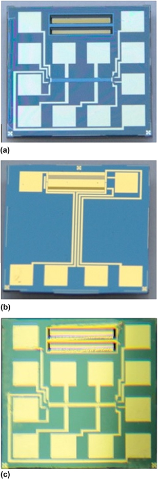
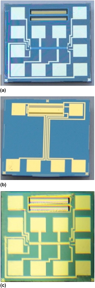
The setup consists of two parts, the prestructured chip (Figs. 1[a]–1[c]) and a suitable measurement environment (see Fig. 2). The chip is combining a hot stripe measurement setup (see Fig. 6) for the Völklein method Reference Völklein, Reith and Meier23–Reference Stärz, Schmidt and Völklein25 for either steady state or transient thermal conductivity, emissivity, and heat capacity measurements with a 4-point measurement setup (Fig. 7) for the determination of the electrical transport properties as well as the Seebeck coefficient. For an easy sample preparation, the front side of the chip is prestructured with a photolithographically defined deposition mask. If this organic mask is not suitable for any reason, like elevated deposition temperatures, an alternative metal shadow mask can be used instead. This configuration allows for a nearly simultaneous characterization of a sample which has been prepared by either PVD (e.g., thermal evaporation, sputtering, MBE), or CVD (e.g., ALD), in one step. As physical properties vary considerably with changing temperature, it is worth mentioning that the chip can easily be used in the scheduled range from 120 to 450 K.
(a) Front view of chip with window structure for the thermal conductivity measurement, Hall-bar structure and organic deposition mask. (b) Back side of the chip with the two membrane setup, including heating stripes. (c) ZT-Chip with deposited sample.
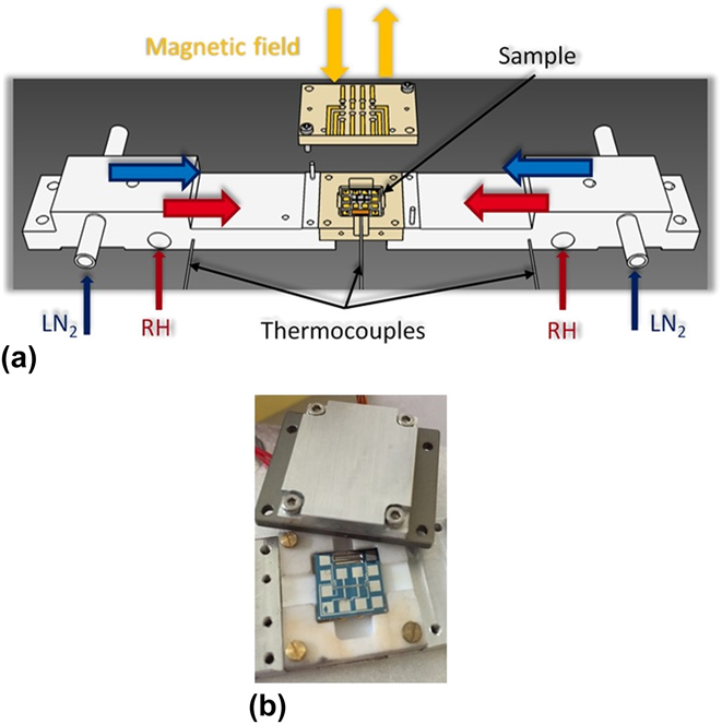
(a) Temperature and magnetic field treatment of the sample (b) sample holder with spring pin contacts and measurement chip inserted.
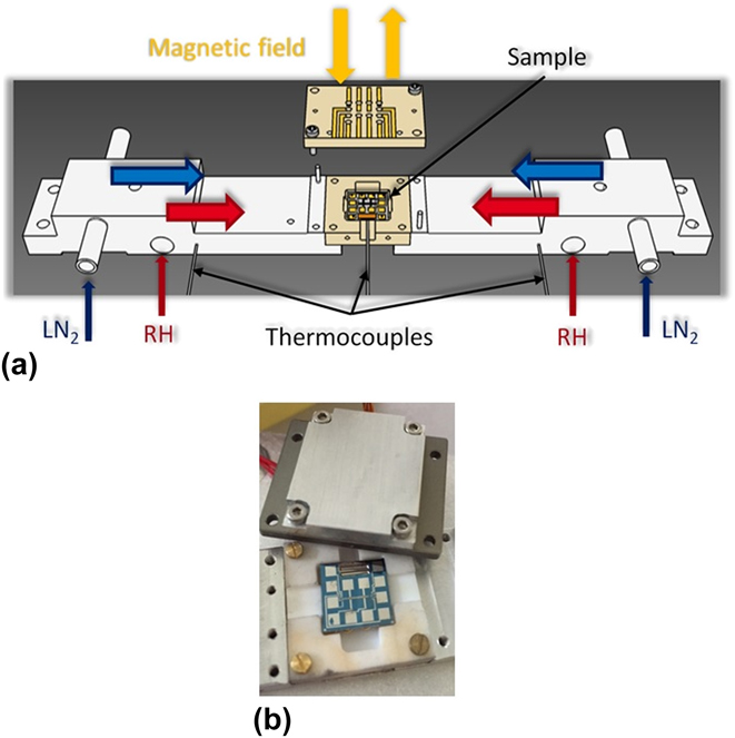
To provide the required environmental conditions like a high vacuum of 10−5 mbar, elevated measurement temperatures, as well as the possibility to apply a magnetic field, a suitable measurement chamber has been designed. The temperature regulation is performed by two PID controlled resistance heaters [RH, see Fig. 2(a)] on both ends of the sample holder, in combination with a thermocouple next to each of them. If necessary, the maximum operating temperature range can be increased to 100 up to 525 K. The maximum range is not used for this work, as the temperature regulation below 120 K gets more unstable at the lower end and the published data for the verification stopped at 450 K at the higher end. The sample temperature is measured with a third thermocouple, located directly under the measurement chip. For an easy device preparation but also as a heat shield, a unique sample holder has been designed to avoid heat loss by radiation and particularly time consuming bonding steps to apply electrical contacts. For the high number of measurement tasks and regulations, optimized measurement electronics and software have been created.
III. FABRICATION OF THE MEASUREMENT CHIPS
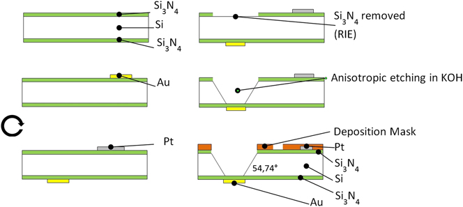
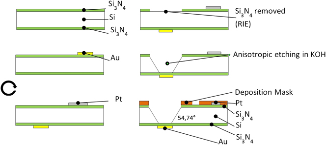
The measurement chip is fabricated in a clean room process, using several lithographic structuring and deposition steps as well as reactive ion etching (RIE) and anisotropic etching of silicon (Fig. 3). As substrate, a 300 µm thick 4 inch (1-0-0) silicon wafer with 100 nm LPCVD Si3N4 layers on both sides is used. In the first step, the heater/sensor stripes for the thermal conductivity measurement are created on the back side of the wafer by photolithographic structuring and subsequent etching of a previously deposited 5 nm/100 nm thick Cr/Au layer. In the next step, the front side electrodes for the Hall-bar and Seebeck measurements are prepared by photolithographic structuring of a 5 nm/100 nm Cr/Pt layer. Pt is used instead of gold to avoid diffusion of the electrode material into the sample at elevated temperatures. Then, two rectangular windows of about 5.5 × 0.75 mm2 and 5.5 × 0.9 mm2 respectively are structured on the topside using photolithographic alignment and reactive ion etching (RIE) of the Si3N4 layer. Afterward, the two windows in the back side nitride layer are prepared as self-supporting membranes by anisotropic etching of the wafer from the front side by applying a KOH solution at 80 °C. Before the measurement chip can be used, a sample deposition mask is placed on the front side of the chip by exposing and developing a negative resist.
Flow chart for the production of the ZT-chips.
IV. SAMPLE PREPARATION
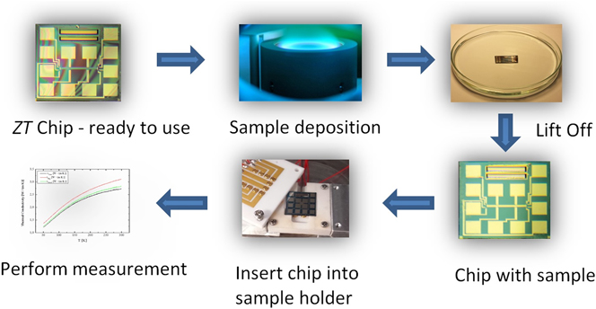
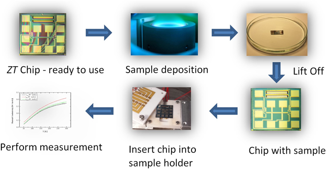
For a reasonable measurement result, some conditions have to be fulfilled. First, the thickness of the sample has to be homogeneous and the sample surface has to be consistently closed. Furthermore, the sample geometry and contacts have to be defined as accurately as possible, as they directly influence the result. This can be achieved by the prestructured organic deposition mask. The sample can simply be deposited onto the chip followed by a lift off step to receive a defined sample structure and to remove excess residuals (see Fig. 4). The organic deposition mask is well suited for most evaporation and sputtering processes, but also for many ALD processes. Nevertheless, limitations of this procedure are elevated deposition temperatures (>120 °C). For these applications, a metallic shadow mask can be used.
Routine for sample preparation and measurement.
In case Si3N4 as a substrate is not suitable, it is also possible to work with a buffer layer in between, which can help to improve the sample growth conditions. The thickness and behavior of the buffer layer then has to be taken into account during the evaluation of the measured data.
V. MEASUREMENT PROCEDURES
A. Thermal conductivity
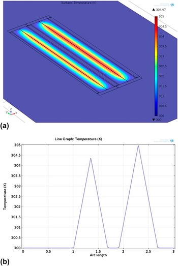
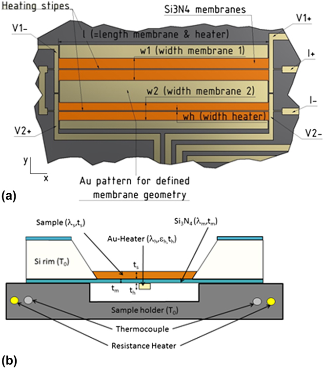
To determine the thermal conductivity λ and emissivity ε of thin films, an advanced setup based on the setup presented by Völklein et al. Reference Völklein, Reith and Meier23 is used (Fig. 6). For the measurement, two thin heating/sensor stripes with a width <5 µm are deposited on the respective back side of the two free standing Si3N4 membranes with the same length but different width. The nitride is used as a suspended substrate but also as a dielectric layer for the separation of conductive samples to the heater. For highest reproducibility and to avoid additional geometry measurements, an Au rim surrounding the membranes has been added to correct uncertainties in the membrane size, which can occur after the etching step because of tolerances in the wafer thickness or deviations of the etching time. The heat sink condition of the thin film Au rim has been validated by a Comsol Multiphysics simulation [Figs. 5(a) and 5(b)].
(a) Temperature distribution of the heated two membrane setup including thin film Au surrounding for geometry definition (b) temperature distribution along the x-axis of the chip, showing the peak temperature of the two heaters and a negligible temperature rise of the Au rim.

(a) Schematic back side view of the chip, showing the hot stripe setup with the two membranes. (b) Schematic cross sectional view and measurement setup of chip on sample holder.
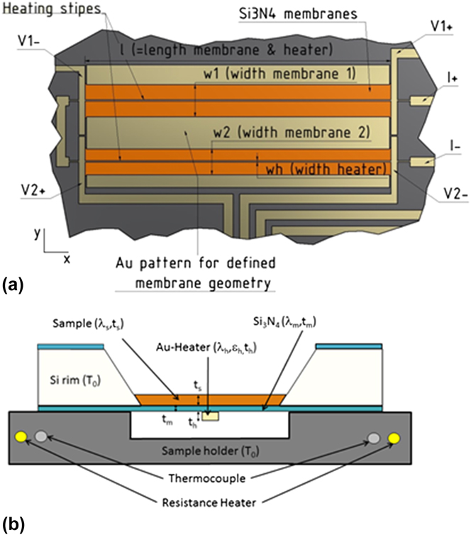
A membrane as thin as possible is very important for the thermal conductivity measurement, as the parasitic heat flux through the substrate is a big issue for in-plane measurements. For sufficient measuring accuracy, the product of the sample thermal conductivity λs and sample thickness t s should be equal to or higher than the corresponding product λm t m of the substrate.
For the measurement, both stripes are heated due to Joule heating by applying a DC current I with the heating power N i = I 2 R i , where R i denotes the resistance of the corresponding heating stripe (i = 1, 2). For the calculation of the thermal conductivity of the sample, the 2D partial differential heat equation has been solved, and with respect to the boundary conditions and simplifications, the thermal conductance G is given by Reference Völklein, Reith and Meier23 :
 $$G\left[ {1 - {2 \over {\upsilon l}}\tanh \left( {\upsilon {l \over 2}} \right)} \right] = {G_{\rm{m}}}\left( {\lambda ,\varepsilon } \right) + {G_{\rm{h}}}\left( {{\varepsilon _{\rm{h}}}} \right)\quad ,$$
with
 $$\upsilon {l \over 2} \approx \sqrt {{{{G_{\rm{m}}}\left( {\lambda ,\varepsilon } \right) + {G_{\rm{h}}}\left( {{\varepsilon _{\rm{h}}}} \right)} \over {{{4{\lambda _{\rm{h}}}{t_{\rm{h}}}{w_{\rm{h}}}} \mathord{\left/ {\vphantom {{4{\lambda _{\rm{h}}}{t_{\rm{h}}}{w_{\rm{h}}}} l}} \right. \kern-\nulldelimiterspace} l}}}} \quad .$$
G m is the thermal conductance of the sample plus membrane due to heat conduction and radiation, G h is the thermal conductance of the heater due to radiation, and G is the thermal conductance of the chip including sample and can be obtained using
 $$G = {N \over {\Delta {T_{\rm{M}}}}}\quad ,$$
where ΔT M is the mean temperature increase caused by the heating power N and is correlated to the change in resistance by the temperature coefficient of resistance β
 $$\Delta {T_{\rm{M}}} = {{R\left( {{T_0} + \Delta {T_{\rm{M}}}} \right) - R\left( {{T_0}} \right)} \over {\beta R\left( {{T_0}} \right)}}\quad ,$$
where R(T 0 + ΔT M) and R(T 0) denote the resistance of the heated and unheated stripe, respectively. The measurement is performed in high vacuum (P < 10−5 mbar), therefore the convective heat loss can be neglected and only the dissipated heat caused by thermal conductance and radiation has to be considered. The heat loss due to radiation from the heating stripe to the environment can be calculated by
 $${G_{\rm{h}}}\left( {{\varepsilon _{\rm{h}}}} \right) = 8{\varepsilon _{\rm{h}}}{\sigma _{\rm{B}}}T_0^3{w_{\rm{h}}}l\quad ,$$
where εh is the emissivity of Au, σB is the Stefan–Boltzmann constant, T 0 is the ambient temperature, w h is the width and l the length of the heater. By iteratively solving Eq. (1), the thermal conductance G m (λ, ε) of the sample plus membrane can be calculated. Since the conductance depends on λ and the emissivity ε, it is necessary to measure at least two samples with differing geometries (w 1, w 2) to determine its thermal conductivity and emissivity using
 $$\lambda t = {{{G_{\rm{m}}}\left( {{w_1}} \right)\tanh \left( {\mu {{{w_1}} \over 2}} \right)} \over {2l\mu }} = {{{G_{\rm{m}}}\left( {{w_2}} \right)\tanh \left( {\mu {{{w_2}} \over 2}} \right)} \over {2l\mu }}\quad ,$$
where
 $${\mu ^2} = {{8\varepsilon {\sigma _{\rm{B}}}T_0^3} \over {\lambda t}}$$
is determined by the numerical solution of
 $${G_{\rm{m}}}\left( {{w_1}} \right)\coth \left( {\mu {{{w_2}} \over 2}} \right) - {G_{\rm{m}}}\left( {{w_2}} \right)\coth \left( {\mu {{{w_1}} \over 2}} \right) = 0\quad .$$
The calculated result is the thermal conductivity λ times thickness t of the sandwich system Si3N4 plus sample with the total thickness t = t s + t m. The sample thermal conductivity is given by
 $${\lambda _{\rm{s}}} = {{\lambda t - {\lambda _{\rm{m}}}{t_{\rm{m}}}} \over {{t_{\rm{s}}}}}\quad .$$
Sikora et al. Reference Sikora, Ftouni, Richard, Hébert, Eon, Omnès and Bourgeois16,Reference Sikora, Ftouni, Richard, Hébert, Eon, Omnès and Bourgeois26 and Ftouni et al. Reference Ftouni, Tainoff, Richard, Lulla, Guidi, Collin and Bourgeois27 showed, that the presented setup can be applied not only for steady-state measurements, but also for transient measurements of the in-plane thermal conductivity and additional specific heat capacitance using the 3ω technique. In this case, instead of a DC current, an AC current I = I 0 cos(ωt) is applied to one of the two heating stripes, causing a temperature rise of the membrane in the form of ΔT = ΔT 0 cos(2ωt + φ) and consequentially an oscillation in the resistance of the stripe R = R 0(1 + βΔT), at the angular frequency of 2ω. With regard to the frequency, the phase shift φ depends on both, the geometry of the heater and the underlying materials. By measuring the voltage drop across the heater, according to Ohms law V = RI, one gets an amplitude modulated signal which has a small component at the third harmonic 3ω, which can be extracted with a lock-in amplifier.
By solving the 2D partial differential heat equation across the membrane with regard to the given boundary conditions, it can be shown Reference Sikora, Ftouni, Richard, Hébert, Eon, Omnès and Bourgeois16,Reference Völklein, Reith and Meier23 that the amplitude of the temperature oscillation is given by
 $$\Delta {T_{\rm{M}}} = {{{N_0}} \over {{K_{\rm{P}}}\sqrt {1 + {\omega ^2}\left( {4{\tau ^2} + {{{w^4}} \over {24{D^2}}} + {{\tau {w^2}} \over {3D}}} \right)} }}\quad ,$$
with the mean dissipated heating power N 0 = RI 0 2/2, the width of the membrane w, the thermal diffusivity of the sample plus membrane setup D = λ/ρc, where ρ is the mass density and c the specific heat capacity, the angular frequency ω, K P = 2λtl/w and the thermal relaxation time τ = C′/K P. Using Eqs. (3) and (10), the general expression for the amplitude of the 3ω oscillation V 3ω is given by
 $$\left| {{V_{3\omega }}} \right| = {{\beta R_0^2I_0^3} \over {4{K_{\rm{P}}}\sqrt {1 + {\omega ^2}\left( {4{\tau ^2} + {{{w^4}} \over {24{D^2}}} + {{\tau {w^2}} \over {3D}}} \right)} }}\quad .$$
The thermal conductivity λ and specific heat capacity c of the membrane or membrane plus additional sample can be extracted by fitting the 3ω voltage data versus the frequency using Eq. (11). The sample's thermal conductivity can be calculated using Eq. (9) and the specific heat can be obtained, using the densities ρ of the materials involved, by subtracting the known membrane values from those of the sandwich system.
 $$C' = {\rho _{{\rm{Au}}}}{c_{{\rm{Au}}}}{t_{\rm{h}}}{{{w_{\rm{h}}}} \over 2}l + {\rho _{{\rm{S}}{{\rm{i}}_3}{{\rm{N}}_4}}}{c_{{\rm{S}}{{\rm{i}}_3}{{\rm{N}}_4}}}{t_{\rm{m}}}{{{w_{\rm{h}}}} \over 2}l + {\rho _{\rm{s}}}{c_{\rm{s}}}{t_{\rm{s}}}{{{w_{\rm{h}}}} \over 2}l\quad .$$
B. Electrical conductivity and hall coefficient
To determine the electrical conductivity (σ) and Hall coefficient (A H) of the sample, a Hall-bar setup Reference Zastrow, Gooth, Boehnert, Heiderich, Toellner, Heimann, Schulz and Nielsch9 has been structured on the chip. The bar shaped geometry of the sample is formed by a photolithographically defined mask with only few µm uncertainty compared to a millimeter scale sample size. For a good measurement result, the thickness of the sample must be homogeneous and has to be measured as precise as possible.
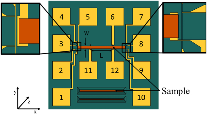
In Fig. 7 the front side of the measurement chip is presented. For the electrical conductivity measurement, a current is applied between pads 5 and 8 and the occurring voltage drop between pads 11 and 12 is measured. The conductivity can be calculated using
 $$\sigma = {{{I_{5,8}}L} \over {{V_{11,12}}W{t_{\rm{s}}}}}\quad ,$$
where W and t s are the width and thickness of the sample and L is the distance between the contacts 11 and 12. To minimize the measurement error, further measurements are taken by reversing the current and voltage. The measured voltages are summed up with respect to their sign and divided by the number of measurements.
Front side of the measurement chip with deposited sample.
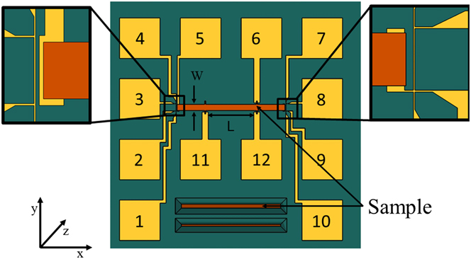
For the Hall coefficient measurement, the corresponding Hall voltage V Hall can be measured between pads 12 and 6, by applying a current I 5,8 between pads 5 and 8 and a magnetic field B z perpendicular to the sample surface. It can then be calculated using
 $${A_{\rm{H}}} = {{{V_{{\rm{Hall}}}}{t_{\rm{S}}}} \over {{I_{5,8}}{B_{\rm{Z}}}}}\quad .$$
C. Seebeck coefficient
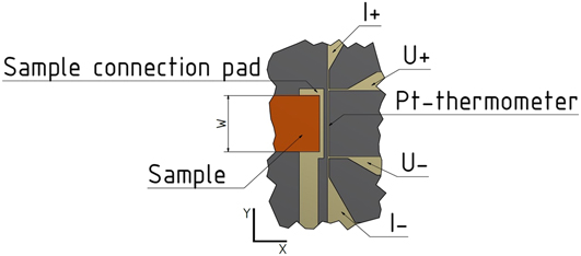
For the determination of the samples Seebeck coefficient, the Hall-bar structure is used. As the same contacts are used, it is not possible to take the resistivity and Seebeck measurement simultaneous, but successively. In addition to the Hall-bar contacts, two resistance thermometers are located directly at the intersection between sample and measurement pad (see Figs. 7 and 8). Their resistance is measured in a 4-point configuration using the pads 1, 2, 3, 4 (T 1) and 7, 8, 9, 10 (T 2). The thermometer material is platinum and the geometry is designed to have a resulting resistance of about 100 Ω at room temperature (R T). The temperature coefficient of resistance of the thermometer is measured using the thermocouple directly under the chip at thermal equilibrium conditions during the measurement routine [Fig. 2(a)].
 $${T_1} \propto {{{V_{2,3}}} \over {{I_{1,4}}}}{\rm{\ }}\amp {\rm{\ }}{T_2} \propto {{{V_{8,9}}} \over {{I_{7,10}}}}\quad .$$
Seebeck measurement setup with a resistance thermometer at each side (details of one side).
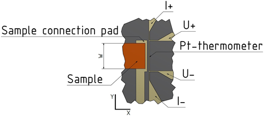
The Seebeck measurement is performed, by applying various temperature gradients in the x-direction of the chip and measuring the temperature difference ΔT = T Hot − T Cold, as well as afterward the thermoelectric voltage V th between the two intersections, using pads 5 and 8 (Fig. 7). The temperature gradient is created by heating one side of the sample holder. The Seebeck coefficient can then be calculated using
 $$S - {S_{{\rm{Pt}}}} = {{ - {V_{{\rm{th}}}}} \over {{T_{{\rm{Hot}}}} - {T_{{\rm{Cold}}}}}}\quad .$$
where S Pt denotes the Seebeck coefficient of the platinum contact lines.
VI. DISCUSSION
For the validation and to show the capability of the platform, a well-known and already characterized thermoelectric material has been chosen. Völklein et al. Reference Völklein and Kessler28,Reference Völklein and Kessler29 already published measurements for bismuth-antimony thin film alloys with regard to their antimony concentration and film thickness.
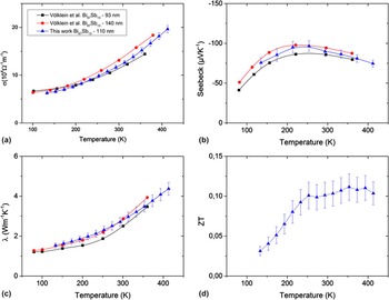
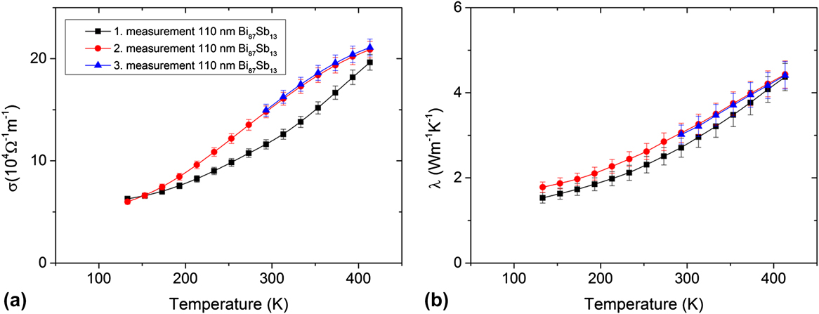
For the showcase study, a 110 nm thin Bi87Sb13 film, which was deposited by high vacuum thermal evaporation, has been measured in the temperature range from 120 K up to 450 K and the results have been compared to the published data (Figs. 9[a]–9[d]). This measurement has been repeated in a second measurement run from 120 K to 450 K and a third measurement run from RT to 450 K to show the reproducibility of the platform.
Comparison of the electrical (a) and thermal (b) conductivity as well as the Seebeck coefficient (c) of Bi87Sb13 thin films measured by Völklein et al. Reference Völklein and Kessler28,Reference Völklein and Kessler29 with this work as well as the resulting ZT value (d) in the temperature range between 120 K and 450 K.

The comparison of the measurements shows a very good agreement to the previously published data. A maximum ZT value of 0.11 at 350 K has been obtained.
In addition, reproducibility tests have been performed, which show the advantage of the nearly simultaneous measurements of different parameters at the same sample. Because of the heating during the first measurement, thermal annealing effects occurred, which can be seen in Figs. 10(a) and 10(b). The data for the second and third measurement run show significant changes in the thermal and electrical transport properties after the sample was heated up to 450 K during the first run.
Reproducibility of the electrical (a) and thermal (b) conductivity measurements of a 110 nm Bi87Sb13 thin film in the temperature range between 120 K and 450 K.

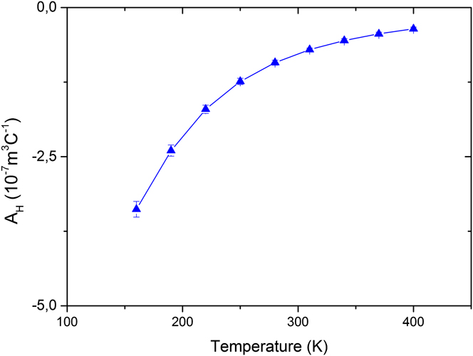
Beside the thermoelectric properties σ, λ, and S, the Hall coefficient A H has been measured in a magnetic field which was applied perpendicular to the sample surface (Fig. 11). The magnetic field strength was sweeped from −1 T to +1 T at constant ambient temperatures T 0. The Hall resistance R H was calculated using the slope ΔV H/ΔB to avoid offset errors.
Hall coefficient of a 110 nm Bi87Sb13 thin film in the temperature range between 120 K and 450 K.

The measurement results are in good agreement with literature data and can be used for detailed analysis of the transport properties. Further calculations of charge carrier concentration and mobility can be achieved by applying an anisotropic two-carrier model. Reference Völklein and Dillner30
VII. CONCLUSIONS
A viable platform for the in-plane ZT characterization of thin films has been developed. It consists of a measurement chip, which acts as a substrate for the sample deposition, and an optimized chamber with sample holder to generate flexible environmental conditions in terms of temperature and magnetic field. The Si-based measurement chips are prestructured and already equipped with the required measurement setups to perform a complete in-plane ZT characterization of the sample. Because of the nearly simultaneous measurement of the physical parameters from the same sample within one measurement run, the results are directly comparable and can be used for the in-plane ZT characterization. The prestructured deposition mask and the sample holder design minimize the effort for the sample preparation.
The validation of the platform has been provided by the comparison of measured data of a 110 nm thick Bi87Sb13 thin film sample with the results of previously published data by Völklein et al. Reference Völklein and Kessler28,Reference Völklein and Kessler29 A maximum in-plane ZT value of about 0.11 at 350 K has been calculated. Moreover, the reproducibility of the platform has been proved and the influence of thermal annealing during a measurement run has been observed. This underlines the advantage of the nearly simultaneous measurements of all physical properties.
Further potential for improvements of the measurement capabilities is given by the consideration of the Nernst–Ettinghausen effect, as the setup is able to perform measurements at the sample under the presence of both, a heat flux and a magnetic field perpendicular to it. More accurate Hall-mobility and carrier concentration measurements could be achieved by isolating this effect. In addition, further information, such as the carrier effective mass can be calculated from the Nernst coefficient, along with the measured resistivity, Seebeck coefficient, and Hall coefficient. Reference Coutts, Young, Li, Mulligan and Wu31–Reference Young, Coutts, Kaydanov, Gilmore and Mulligan34