1 Introduction
The turbulent/non-turbulent interface (TNTI) is the thin but sharp interfacial layer that separates fluid with high vorticity from an adjacent region fluid with low vorticity (Mathew & Basu Reference Mathew and Basu2002; Westerweel, Fukushima & Pedersen Reference Westerweel, Fukushima, Pedersen and Hunt2009). The multi-scale nature of turbulent eddies act to increase the surface area of the TNTI through wrinkling and deformation. The relationship between the wrinkled surface of the TNTI, the local turbulent structure and entrainment processes are of fundamental importance if we wish to understand the mechanisms responsible for the growth of turbulent regions into the non-turbulent regions. A better understanding of the local processes that control mass transport has widespread practical importance in science and engineering.
The TNTI plays an important role in the entrainment process because it is within the finite thickness of the TNTI that vorticity and scalars are diffused into the non-turbulent fluid (Corrsin & Kistler Reference Corrsin and Kistler1955; van Reeuwijk & Holzner Reference van Reeuwijk and Holzner2014; Taveira & da Silva Reference Taveira and da Silva2014). Although viscous diffusion and molecular diffusion are slow, they are expedited by an increase in the surface area of the TNTI in both homogeneous and variable density flows (Mathew & Basu Reference Mathew and Basu2002; Krug, Holzner & Lüthi Reference Krug, Holzner, Lüthi, Wolf, Kinzelbach and Tsinober2015). In the more complex case of turbulent reacting flows, modification of the flame surface area strongly affects the local reactant consumption rate in a similar way (Trouvé & Poinsot Reference Trouvé and Poinsot1994).
The proposition that the area of a turbulent surface,
 $S$
, such as the TNTI, follows a power-law scaling of the form,
 $S\sim \unicode[STIX]{x1D6E5}^{2-D_{f}}$
, where the
 $D_{f}$
represents the true three-dimensional fractal dimension and
 $\unicode[STIX]{x1D6E5}$
is the side length of a cube, was first proposed by Sreenivasan & Meneveau (Reference Sreenivasan and Meneveau1986). Invoking both Reynolds similarity hypothesis and Kolmogorov scaling predicts a universal fractal dimension of
 $D_{f}=2+1/3$
for turbulent surfaces within the inertial range of scales. Current experimental methods are incapable of suitably resolving the multi-scale surface area of the TNTI and therefore direct evaluation of
 $D_{f}$
remains out of reach. However, the apparent fractal dimension can be inferred from well-resolved two-dimensional data. Like measuring the coastline of land masses, the length of the TNTI depends on the observed spatial resolution and it is only recently that high-resolution, multi-scale experimental techniques have become available. Therefore to test the validity of the power-law scaling we evaluate the length, rather than the surface area, of the TNTI which varies as
 $L\sim \unicode[STIX]{x1D6E5}^{1-D}$
. Thus the expected two-dimensional fractal dimension
 $D$
obtained from measured intersections with a plane is
 $D=1-M$
, where the exponent
 $M$
may be estimated by measuring the local slope,
 $m(\unicode[STIX]{x1D6E5})$
, of the logarithm of the interface length,
 $L_{s}$
, as a function of the logarithm of the spatial filter size
 $\unicode[STIX]{x1D6E5}$
; this exponent is predicted to be
 $M=-1/3$
giving
 $D=1+1/3$
. The apparent surface area scaling of
 $D_{f}=2+1/3$
can then recovered by invoking Mandelbrot’s additive law (Mandelbrot Reference Mandelbrot1982).
Recent experimental studies by de Silva, Philip & Chauhan (Reference de Silva, Philip, Chauhan, Meneveau and Marusic2013) in high Reynolds number boundary layers and in the far field of axisymmetric jets by Mistry, Philip & Dawson (Reference Mistry, Philip, Dawson and Marusic2016) have found that
 $m(\unicode[STIX]{x1D6E5})$
lies in the range of
 $-0.3$
to
 $-0.4$
, resulting in a corresponding fractal dimension of
 $D=1.3{-}1.4$
that is consistent with the theoretical value of
 $D=1+1/3$
. Similar observations were reported in a recent direct numerical simulation (DNS) of a turbulent boundary layer by Borrell & Jiménez (Reference Borrell and Jiménez2016). The fact that similar values for
 $D$
have been reported in wall bounded and free shear flows is of significance. Fractal scaling has also recently been demonstrated to be a feature of turbulent premixed flames in certain flame regimes (Chatakonda, Hawkes & Aspden Reference Chatakonda, Hawkes, Aspden, Kerstein, Kolla and Chen2013), and can provide a framework for subgrid models for large eddy simulations (Charlette, Meneveau & Veynante Reference Charlette, Meneveau and Veynante2002; Hawkes, Chatakonda & Kolla Reference Hawkes, Chatakonda, Kolla, Kerstein and Chen2012). Given the importance of turbulent interfaces in science and engineering, understanding how the scaling of the TNTI evolves in a canonical, homogeneous flow, such as an axisymmetric jet, can offer insight that can be applied to more complex and technically important flows. In this paper we investigate the evolution of the power-law behaviour of the TNTI in the near field of a turbulent jet where the turbulent statistics have yet to achieve self-similarity.
The paper is structured as follows. In §§ 2 and 3 we describe the apparatus, experimental methods and techniques used to identify the TNTI. In § 4 we apply a multi-scale analysis based on spatial filtering of the scalar concentration fields to test the power-law scaling by evaluating how the length of the TNTI varies with filter size over two decades of scale separation. Finally, in § 5, we demonstrate that the evolution of the fractal dimension using an exact fractal construction of a Koch curve exhibits similar behaviour to the developing scale separation in the near field of the jet.
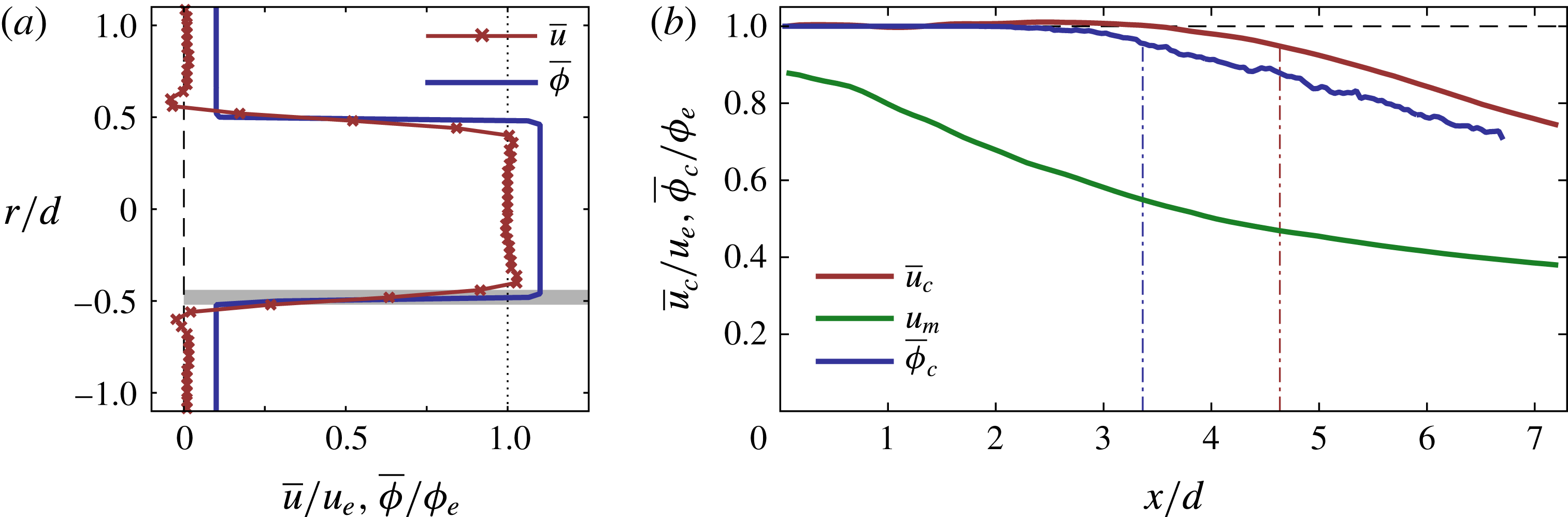
(a) Nozzle-exit velocity profile (red) and scalar concentration profile (blue). The scalar profile is shifted by
 $+0.1\unicode[STIX]{x1D719}_{e}$
for clarity. The resolution of the PIV measurement is illustrated by the filled grey region. (b) The profiles of the mean centreline velocity (red), integral velocity (green) and centreline scalar concentration (blue). The potential core lengths are denoted by the vertical dashed lines.

2 Experimental methods
A free turbulent jet was produced in a
 $8\times 0.9\times 0.5~\text{m}$
water tank. The Reynolds number of the jet is
 $Re=24\,000$
, where
 $Re=u_{e}d/\unicode[STIX]{x1D708}$
,
 $u_{e}=0.60~\text{m}~\text{s}^{-1}$
is the nozzle-exit velocity,
 $d=40~\text{mm}$
is the diameter of the jet and
 $\unicode[STIX]{x1D708}=1\times 10^{-6}~\text{m}^{2}~\text{s}^{-1}$
is the kinematic viscosity. The exit velocity and scalar profiles are close to top hat as shown in figure 1(a).
High-speed, simultaneous particle image velocimetry (PIV) and planar laser induced fluorescence (PLIF) were used to measure the velocity and scalar fields in the near-field region of the jet. A single high-speed laser (Quantronix Darwin-Duo 527-60-M, 527 nm) was used for both PIV and scalar measurements. For the scalar measurements, a reservoir containing an aqueous solution of fluorescent dye (rhodamine 6G) was fed to the jet and discharged into clean water. Both the dyed and clean water were seeded with neutrally buoyant
 $20~\unicode[STIX]{x03BC}\text{m}$
particles for the PIV measurements. Optical filters were used to isolate the dye fluorescence signal at 555 nm for the PLIF camera and the Mie scattering at 527 nm for the PIV cameras.
Two PIV cameras (
 $1024\times 1024$
pixels) were positioned side-by-side in a stitched configuration extending the field-of-view (FOV) to capture approximately
 $7d$
in streamwise direction. The measurement FOV is
 $-1.8\leqslant r/d\leqslant 1.8$
and
 $0\leqslant x/d\leqslant 6.8$
in the radial (
 $r$
) and streamwise (
 $x$
) directions respectively. Particle images were acquired every
 $\unicode[STIX]{x1D6FF}t=1.0~\text{ms}$
and processed using a PIV cross-correlation algorithm that included multi-passes of decreasing window size with a final interrogation window size of
 $24\times 24~\text{pixels}$
with 75 % window overlap. Window-shift and window-deformation features were implemented to improve accuracy (Adrian & Westerweel Reference Adrian and Westerweel2011). The final vector fields have a spatial resolution of 3.20 mm (
 $0.08d$
) and vector spacing of 0.80 mm (
 $0.02d$
).
A single PLIF camera (
 $1024\times 1024$
pixels) was used to capture the same FOV of the PIV measurements. An image post-processing technique, previously described in Mistry et al. (Reference Mistry, Philip, Dawson and Marusic2016), was implemented to convert the raw PLIF images into a scalar field in which the image intensity is linearly proportional to the local scalar concentration. Post-processing included compensation for the non-uniform laser intensity profile along the image plane and absorption along the beam path. Linearity of the fluorescence signal with concentration and non-uniformities in the laser intensity profile were determined and characterised by imaging a dye cell containing homogeneous solutions of rhodamine 6G of different concentration. The instantaneous PLIF images were then integrated along the laser beam path to account for absorption according to the Beer–Lambert law (Crimaldi Reference Crimaldi2008). The intensity profiles were corrected along columns in the PLIF image rather than along the beam path as the laser sheet is very slowly expanding and therefore the beam paths are close to being vertical. The resulting scalar concentration fields have a pixel spacing of 0.26 mm (
 $0.0065d$
). A total of
 $10\,912$
vector and scalar fields were recorded and the results presented in this paper are calculated using 500 down-sampled fields. An example of an instantaneous scalar concentration field is presented in figure 6(a).
The top-hat velocity profile at the nozzle exit is illustrated in figure 1(a), in which the axial velocity only varies by
 $\pm 3\,\%$
in the region
 $r/d\pm 0.4$
. The velocity step profile between the ambient region and the jet flow is smoothed due to the finite spatial resolution of the PIV measurements. The PIV spatial resolution is shown by the grey bar in figure 1(a). The scalar concentration profile of the passive dye (blue line) in figure 1(a) shows a top-hat profile that exhibits a step change at
 $r/d=\pm 0.5$
. The centreline velocity and scalar concentration profiles in figure 1(b) illustrate the length of the potential core of the jet, which is defined as the streamwise distance at which the mean centreline quantity drops to 95 % of the exit value. The potential core length is measured to be
 $4.6d$
and
 $3.4d$
for the velocity and scalar fields, respectively, and the velocity potential core length agrees with comparable near-field studies of axisymmetric jets (Fellouah & Pollard Reference Fellouah and Pollard2009). In figure 1(b) we also plot the integral velocity,
 $u_{m}=M/Q$
, where
 $M=2\int _{0}^{\infty }\overline{u}^{2}r\,\text{d}r$
is the momentum flux and
 $Q=2\int _{0}^{\infty }\overline{u}r\,\text{d}r$
is the volumetric flux; we only evaluate these integrals to the radial extents of the FOV. The decay of
 $u_{m}$
demonstrates that momentum transfer occurs towards the end of the potential core region.
3 Identification of the TNTI
The TNTI represents a finite region separating the turbulent from the non-turbulent regions of the flow and is characterised by a jump in vorticity. We identify the TNTI by applying a threshold procedure from PLIF imaging of a high
 $Sc$
passive scalar that has been used previously (Westerweel et al.
Reference Westerweel, Fukushima, Pedersen and Hunt2009; Mistry et al.
Reference Mistry, Philip, Dawson and Marusic2016). Moreover, PLIF measurements offer greater spatial resolution and dynamic range compared to PIV, which better lends itself to multi-scale analysis of the TNTI surface.
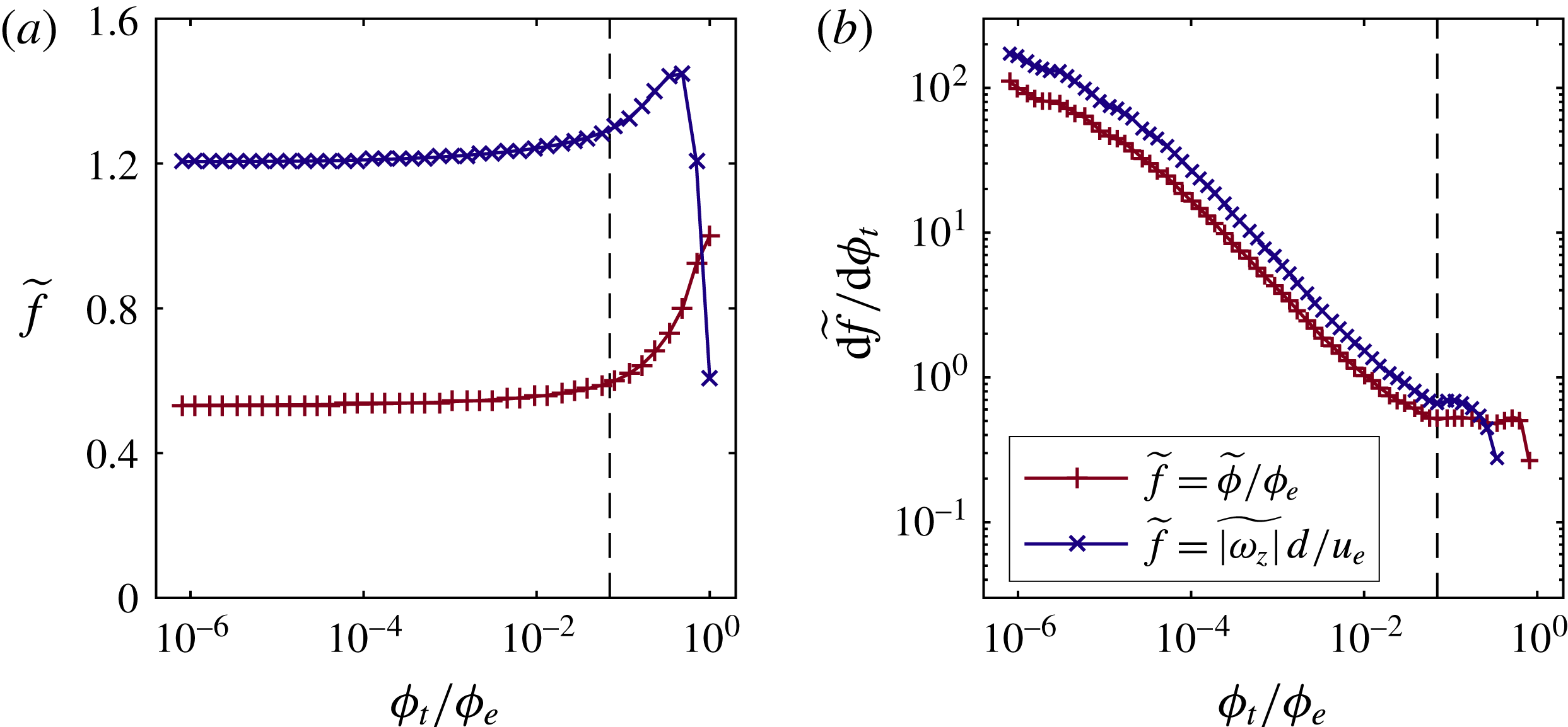
(a) Conditionally averaged scalar concentration (
 $\widetilde{\unicode[STIX]{x1D719}}/\unicode[STIX]{x1D719}_{e}$
, red
 $+$
symbols), and spanwise vorticity magnitude (
 $\widetilde{|\unicode[STIX]{x1D714}_{z}|}d/u_{e}$
, blue
 $\times$
symbols) as a function of scalar threshold,
 $\unicode[STIX]{x1D719}_{t}$
. (b) Gradient of the conditionally averaged profiles shown in (a). The vertical dashed lines indicate the inflection point in the profiles,
 $\unicode[STIX]{x1D719}_{t}/\unicode[STIX]{x1D719}_{e}=0.07$
.

In this section we describe the empirical approach used to identify a scalar concentration threshold that corresponds to the TNTI (Prasad & Sreenivasan Reference Prasad and Sreenivasan1989; Westerweel, Hofmann & Fukushima Reference Westerweel, Hofmann, Fukushima and Hunt2002; Mistry et al.
Reference Mistry, Philip, Dawson and Marusic2016). Conditionally averaged profiles of the scalar concentration and spanwise vorticity magnitude are generated by extracting all the points inside the region that exceed some scalar threshold
 $\unicode[STIX]{x1D719}_{t}$
and calculating the ensemble averages,
 $\widetilde{f}(\unicode[STIX]{x1D719}_{t})=\int (f\,\text{d}a)|_{\unicode[STIX]{x1D719}>\unicode[STIX]{x1D719}_{t}}/\int (\text{d}a)|_{\unicode[STIX]{x1D719}>\unicode[STIX]{x1D719}_{t}}$
, where
 $f$
is one of the aforementioned variables and
 $\int (\text{d}a)$
represents a surface integral across points that satisfy
 $\unicode[STIX]{x1D719}>\unicode[STIX]{x1D719}_{t}$
. This process is repeated for a wide range of scalar thresholds and results in the conditionally averaged profiles shown in figure 2(a). The conditionally averaged vorticity
 $\widetilde{\unicode[STIX]{x1D714}_{z}}$
decreases for
 $\unicode[STIX]{x1D719}_{t}/\unicode[STIX]{x1D719}_{e}>0.5$
because these higher scalar thresholds become concentrated within the constant-velocity potential core region of the jet. The scalar threshold that corresponds to the TNTI is given by the inflection point in the conditionally averaged profiles (Prasad & Sreenivasan Reference Prasad and Sreenivasan1989). Taking the gradient of these profiles provides a clearer illustration of the inflection point and is shown in figure 2(b). The derivative of
 $\widetilde{\unicode[STIX]{x1D714}_{z}}$
becomes negative beyond
 $\unicode[STIX]{x1D719}_{t}/\unicode[STIX]{x1D719}_{e}=0.5$
and these points are not shown on this log-scale plot. Nonetheless, we see that the conditional profiles for
 $\widetilde{\unicode[STIX]{x1D719}}$
and
 $\widetilde{|\unicode[STIX]{x1D714}_{z}|}$
have inflection points at
 $\unicode[STIX]{x1D719}_{t}/\unicode[STIX]{x1D719}_{e}=0.07$
; this threshold is used to identify the TNTI in each instantaneous scalar concentration field measured. We extract the longest continuous contour lines in the
 $r>0$
and
 $r<0$
regions, which represent the TNTI for the top half and bottom half of the jet in the measurement plane, respectively.
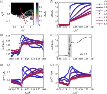
(a) Instantaneous scalar concentration field superimposed with the TNTI (black line) and the interface-normal coordinate
 $x_{n}$
(red vector) at a single point. (b) Averaged profile of scalar concentration along coordinates that are locally normal to the TNTI. The profiles are averaged across
 $x/d\pm 0.5$
intervals based on the streamwise positions indicated in the legend. (c) Averaged profiles of the spanwise vorticity magnitude along
 $x_{n}$
, in logarithmic scaling. (d) Averaged profile of the spanwise vorticity magnitude for
 $x/d\geqslant 4$
in linear scaling. The shaded region denotes the span (
 $0.18d$
) across which the vorticity transitions from non-turbulent to turbulent levels. (e) Root-mean-square (r.m.s.) profiles of scalar concentration along
 $x_{n}$
and (f) r.m.s. profiles of spanwise vorticity magnitude along
 $x_{n}$
.

In this paper we ignore instances of ‘islands’ and ‘holes’ that arise from the intersection of a two-dimensional measurement plane and a three-dimensional scalar field. Islands are defined as pockets of scalar concentration
 $\unicode[STIX]{x1D719}>\unicode[STIX]{x1D719}_{t}$
in the non-turbulent region of the jet and holes are defined as pockets of scalar concentration
 $\unicode[STIX]{x1D719}<\unicode[STIX]{x1D719}_{t}$
in the turbulent region of the jet. A comparison of the area of islands and holes to the total area of turbulent region (i.e. number of points bound by the top and bottom TNTI) shows that islands and holes amount to only 2.2 % and 2.2 % of the total turbulent area, respectively. The measurement of the TNTI length presented in § 4 therefore disregards the isocontours from islands and holes.
Figure 3 shows that isocontours of scalar concentration (
 $\unicode[STIX]{x1D719}/\unicode[STIX]{x1D719}_{e}=0.07$
) delineate the turbulent from the non-turbulent regions of the flow. In this figure we plot ensemble-averaged profiles of (b)
 $\langle \unicode[STIX]{x1D719}\rangle /\unicode[STIX]{x1D719}_{e}$
and (c)
 $\langle |\unicode[STIX]{x1D714}_{z}|\rangle$
along coordinates that are locally normal to the TNTI. This averaging technique evaluates the flow field in a frame of reference that is aligned to the TNTI (Chauhan, Philip & de Silva Reference Chauhan, Philip, de Silva, Hutchins and Marusic2014; Mistry et al.
Reference Mistry, Philip, Dawson and Marusic2016), as illustrated in figure 3(a). Here
 $x_{n}$
represents a coordinate that is locally normal to the TNTI and conditional averages along
 $x_{n}$
are denoted by
 $\langle {\sim}\rangle$
. Figure 3(b) shows that there is a steep increase in the scalar concentration across the TNTI (
 $x_{n}/d=0$
), which is also observed in the far field of turbulent jets (Westerweel et al.
Reference Westerweel, Fukushima, Pedersen and Hunt2009; Mistry et al.
Reference Mistry, Philip, Dawson and Marusic2016). Figure 3(c), presented in logarithmic scaling, shows that there is a corresponding steep increase in vorticity from low levels,
 $O(10^{-2})$
, to high levels,
 $O(10^{0})$
, across the jet boundary. The jump in vorticity is more clearly shown in the linearly scaled plot in figure 3(d); this profile is ensemble averaged using all the profiles in the region
 $x/d\geqslant 4$
. Here, the vorticity jump is centred on the scalar isocontour defining our TNTI (
 $\unicode[STIX]{x1D719}/\unicode[STIX]{x1D719}_{e}=0.07$
) and spans a region of
 $0.18d$
, as denoted by the grey shaded region.
Similar behaviour is also observed when plotting root-mean-square (r.m.s.) quantities, as shown in figure 3(e,f). The scalar r.m.s. profiles in figure 3(e) show the expected jump profile of the variances across the TNTI (
 $x_{n}/d=0$
). Likewise, the r.m.s. spanwise vorticity also shows a rapid increase occurs across the TNTI. In summary, the scalar concentration threshold that we identify in figure 2 yields scalar isocontours that fall within the thin but finite region of the TNTI over which steep changes in vorticity and turbulent quantities occur.
Various studies have shown that the conditional jump profiles for
 $\langle \unicode[STIX]{x1D719}\rangle$
and
 $\langle \unicode[STIX]{x1D714}_{z}^{2}\rangle$
in a
 $Sc\gg 1$
passive scalar field are well correlated across the finite thickness of the TNTI (Prasad & Sreenivasan Reference Prasad and Sreenivasan1989; Westerweel et al.
Reference Westerweel, Fukushima, Pedersen and Hunt2009; da Silva, Hunt & Eames Reference da Silva, Hunt, Eames and Westerweel2014; Watanabe, Sakai & Nagata Reference Watanabe, Sakai, Nagata, Ito and Hayase2015; Mistry et al.
Reference Mistry, Philip, Dawson and Marusic2016). The thickness of the TNTI in shear flows is of the order of the Taylor micro-scale
 $\unicode[STIX]{x1D706}$
, and contains both the viscous superlayer and a turbulent sublayer whose outer boundary is identified by low values of vorticity and concentration. Watanabe et al. (Reference Watanabe, Sakai, Nagata, Ito and Hayase2015) conducted DNS of a temporally evolving mixing layer to investigate the Schmidt number dependence and relationship between the scalar concentration field and the local turbulent mixing across the viscous super layer and turbulent sublayer. Their simulations confirm that the jump in scalar concentration occurs within the finite region of the TNTI for all measured
 $Sc$
numbers (see figure 7a in Watanabe et al.
Reference Watanabe, Sakai, Nagata, Ito and Hayase2015), and that for
 $Sc\gg 1$
, the jump in scalar concentration occurs in the turbulent sublayer which marks the boundary between regions of high and low vorticity. In terms of characterising the surface geometry of the turbulent interface, we are interested in the scale invariance of the TNTI that is predicted to exist in the inertial range and therefore resolving the viscous superlayer structure of the TNTI is not necessary for this purpose.
4 Multi-scale results
We implement a multi-scale methodology to characterise the streamwise evolution of the TNTI geometry. This is achieved by evaluating the scale dependence of the TNTI length using a spatial filtering (‘coarse-graining’) technique previously implemented in turbulent boundary layers and jets (de Silva et al. Reference de Silva, Philip, Chauhan, Meneveau and Marusic2013; Mistry et al. Reference Mistry, Philip, Dawson and Marusic2016). Measurements of the TNTI in these fully developed turbulent flows have been shown exhibit a power-law scaling as a function of measurement resolution, which is characteristic of fractal scaling (Sreenivasan, Ramshankar & Meneveau Reference Sreenivasan, Ramshankar and Meneveau1989).
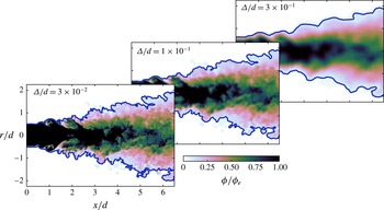
Effect of the spatial filtering on an instantaneous scalar concentration field and corresponding TNTI (blue line). Panels are annotated with the corresponding filter size.

We begin by convolving the scalar concentration fields with box-averaging filters (
 $\widehat{\unicode[STIX]{x1D719}}=\unicode[STIX]{x1D719}\ast G_{\unicode[STIX]{x1D6E5}}$
, where
 $G_{\unicode[STIX]{x1D6E5}}=0$
for
 $|x|,|r|\geqslant \unicode[STIX]{x1D6E5}/2$
, else
 $G_{\unicode[STIX]{x1D6E5}}=1/\unicode[STIX]{x1D6E5}^{2}$
), with filter sizes that span over two decades in length,
 $6.5\times 10^{-3}\leqslant \unicode[STIX]{x1D6E5}/d\leqslant 3.6$
. We spatially filter each of the 500 scalar concentration fields and then identify the corresponding filtered TNTI using a constant threshold value,
 $\unicode[STIX]{x1D719}_{t}/\unicode[STIX]{x1D719}_{e}=0.07$
. An example of the effect of the spatial filtering technique is illustrated in figure 4. The TNTI becomes notably smoother with increasing filter size (left to right), but larger-scale undulations of the interface persist. We then evaluate the ensemble-averaged interface length,
 $\overline{L_{s}}$
, across incremental streamwise extents of size
 $\unicode[STIX]{x1D6FF}x/d=1.5$
, for all filtered images.
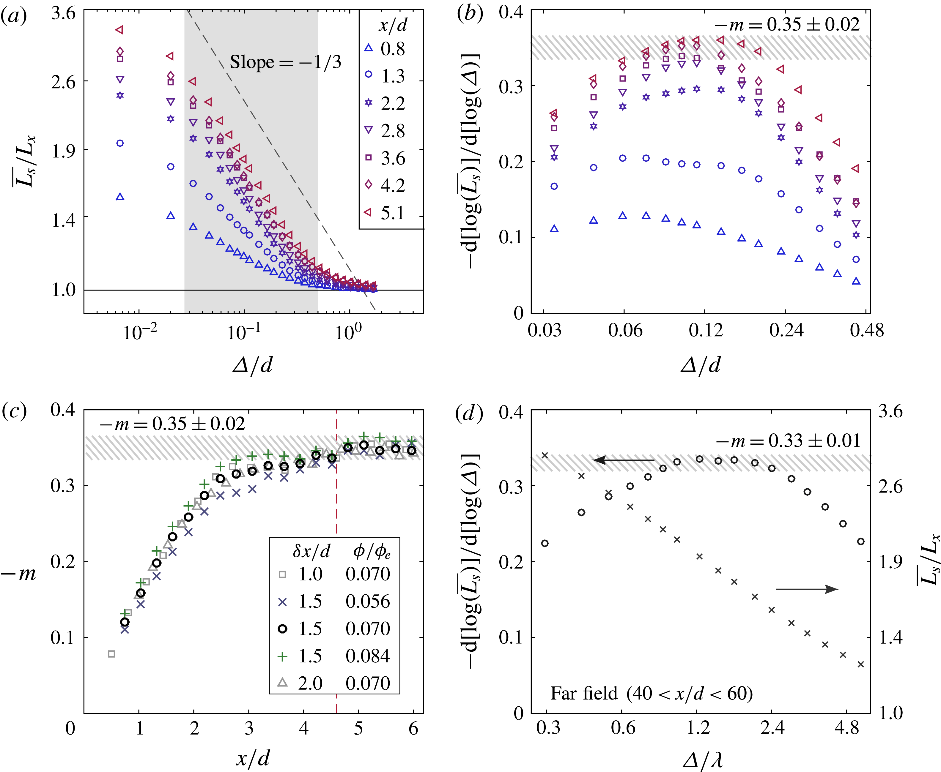
Figure 5(a) shows how
 $\overline{L_{s}}$
varies as a function of filter size over a range of streamwise distances (blue to red symbols, moving downstream) that span the full measurement region. At large filter sizes,
 $\unicode[STIX]{x1D6E5}/d\approx 1$
, the interface is very smooth and essentially one-dimensional. Hence, the mean interface length, normalised by the projected length of the interface
 $L_{x}$
, collapses onto
 $\overline{L_{s}}/L_{x}\approx 1$
. For small filter sizes,
 $\unicode[STIX]{x1D6E5}/d<3\times 10^{-2}$
, the scaling of
 $\overline{L_{s}}/L_{x}$
begins to plateau denoting the end of the fractal scaling. This lower bound of the linear scaling range in figure 5(a,b) is close to the laser sheet thickness (
 $0.04d$
). The upper bound of the scaling range in figure 5(a,b) is approximately
 $\unicode[STIX]{x1D6E5}=0.18d$
, which coincides with the finite thickness of the TNTI that is illustrated in figure 3(d). The linear scaling regime in figure 5(a) can extend below this width because the scalar marker consistently coincides with the centre of the TNTI region (see figure 2
d). At the smallest filter size (
 $\unicode[STIX]{x1D6E5}/d=6.5\times 10^{-3}$
) the interface length ratio of reaches a maximum of
 $\overline{L_{s}}/L_{x}\approx 3.3$
for
 $x/d\geqslant 5$
.
We now estimate the apparent fractal dimension by measuring the slope of the profiles in figure 5(a,b). Note that we refer to
 $D$
as the apparent fractal dimension, in order to distinguish it from the true fractal dimension
 $D_{f}$
, as we only have access to measurements in a two-dimensional plane and therefore cannot directly measure the surface area of the TNTI.
To estimate
 $D$
we use the expression
 $M=1-D$
and estimate the exponent
 $M$
using a measure of the local slope,
 $m(\unicode[STIX]{x1D6E5})$
, of the TNTI length
 $L_{s}$
as a function of filter size,
 $\unicode[STIX]{x1D6E5}$
. It is not straightforward to delineate the slope by applying least-squares fits to the logarithmic profiles in figure 5(a). For example, near the nozzle exit (
 $x/d=0.8$
, blue triangles) the scaling of
 $\overline{L_{s}}$
does not exhibit a discernible linear scaling region. This is more clearly illustrated in figure 5(b) in which we plot
 $m(\unicode[STIX]{x1D6E5})=-\text{d}[\log (\overline{L_{s}})]/\text{d}[\log (\unicode[STIX]{x1D6E5})]$
, for the profiles shown in panel (a). This shows that at
 $x/d=0.8$
, invariant scaling of
 $\overline{L_{s}}$
is not achieved (i.e.
 $m(\unicode[STIX]{x1D6E5})$
is not independent of
 $\unicode[STIX]{x1D6E5}$
). Thus, for streamwise positions close to the nozzle, we may only report a best estimate of
 $M$
which we take as the maximum value
 $m(\unicode[STIX]{x1D6E5})$
in figure 5(b). In the figure, this maximum value is denoted
 $-m$
. The onset of a scale range over which
 $m(\unicode[STIX]{x1D6E5})$
remains invariant is only achieved near the end of the potential core. For example, at
 $x/d=5.1$
there is a finite region of
 $\unicode[STIX]{x1D6E5}/d$
over which the local slope plateaus and does not significantly change.
(a) Scaling of the measured interface length,
 $\overline{L_{s}}$
, as a function of the spatial filter size,
 $\unicode[STIX]{x1D6E5}$
, at different streamwise distances
 $x/d$
. The filled grey area indicates the region over which the local slope is plotted in (b). (b) Local slope of the profiles presented in (a). (c) Evolution of
 $m$
with downstream distance. The hatched region represents
 $-m=0.35\pm 0.02$
which yields an apparent fractal dimension
 $D=1.35\pm 0.02$
. The vertical dashed red line denotes the end of the potential core region based on the centreline velocity. (d) Local slope (
 $\circ$
, left axis) and interface length
 $\overline{L_{s}}$
(
 $\times$
, right axis) of the TNTI measured in the far field between
 $40<x/d<60$
of a round jet (Mistry et al.
Reference Mistry, Philip, Dawson and Marusic2016).

The streamwise evolution of
 $-m$
is plotted in figure 5(c), denoted by the black circles. Note that the streamwise distances in this plot represent the centre points about which incremental segments of
 $x/d\pm 0.75$
(
 $\unicode[STIX]{x1D6FF}x/d=1.5$
) are used to measure
 $-m$
. We observe that
 $-m\approx 0.12$
near the nozzle exit and gradually increases until it reaches a plateau of
 $-m=0.35\pm 0.02$
at
 $x/d>4.6$
which corresponds to
 $D=1.35\pm 0.02$
. The observed plateau of
 $-m$
beyond
 $x/d=4.6$
approximately coincides with the end of the potential core based on the mean centreline velocity (see figure 1
b). These findings are consistent with other fully developed turbulent flows (
 $D=1.3{-}1.4$
, de Silva et al. (Reference de Silva, Philip, Chauhan, Meneveau and Marusic2013); Borrell & Jiménez (Reference Borrell and Jiménez2016); Mistry et al. (Reference Mistry, Philip, Dawson and Marusic2016)) and theory based on the Reynolds number similarity hypothesis (Sreenivasan et al.
Reference Sreenivasan, Ramshankar and Meneveau1989).
For comparison we also present data measured in the far field between
 $x/d=40{-}60$
(see Mistry et al.
Reference Mistry, Philip, Dawson and Marusic2016 for details) in figure 5(d). The abscissa represents the coarse-grain filter size
 $\unicode[STIX]{x1D6E5}$
normalised by the Taylor micro-scale
 $\unicode[STIX]{x1D706}$
measured at the jet centreline at
 $x/d=50$
. The
 $\times$
-markers depict the scaling of
 $\overline{L_{s}}$
and correspond to the right-hand side ordinate axis. The derivative of this profile,
 $m(\unicode[STIX]{x1D6E5})=-\text{d}[\log (\overline{L_{s}})]/\text{d}[\log (\unicode[STIX]{x1D6E5})]$
, is depicted as
 $\circ$
-markers and corresponds to the left-hand side ordinate axis. In the fully developed far field of a jet between
 $x/d=40{-}60$
a distinct linear scaling region was observed over which the slope
 $m(\unicode[STIX]{x1D6E5})$
remains constant at
 $-m=0.33\pm 0.01$
, which is equivalent to a apparent fractal dimension
 $D=1.33\pm 0.01$
.
Introducing the far-field result in figure 5(d) serves to emphasise that the behaviour of the TNTI geometry observed in the self-similar region of the jet is also observed at the end of the potential core as shown by the value of
 $-m=0.35\pm 0.02$
indicated by figure 5(c). The development of fractal scaling
 $D=1.35\pm 0.02$
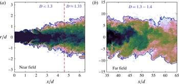
by the end of the potential core is an indication that scale similarity of the interface geometry has been achieved, which arises when the turbulence is sufficiently developed so that the small-scale dynamics is becoming universal rather than dominated by case-dependent large-scale processes. This does not mean that the range of scales at the end of the potential core is as large as the range of scales in the far field, rather that the range of scales at the end of the potential core, however limited, are sufficient to achieve invariance of the interface geometry. Figure 6 compares the TNTI in the (a) near field and (b) far field (see Mistry et al.
Reference Mistry, Philip, Dawson and Marusic2016 for details) of the jet and shows that beyond the potential core (dashed red line), the TNTI is visually similar to that in the fully developed far field.
Instantaneous scalar concentration fields (in logarithmic scaling) of the (a) near field (
 $Re=24\,000$
), and (b) far field (
 $Re=25\,300$
, see Mistry et al.
Reference Mistry, Philip, Dawson and Marusic2016 for details) of axisymmetric jets; each field is scaled differently. The TNTI is denoted by the thick blue line and the end of the potential core in the near field is denoted by the dashed red line.

We include in figure 5(c) a sensitivity analysis of the measured value of
 $-m$
for different incremental streamwise extents,
 $\unicode[STIX]{x1D6FF}x/d=1.0,1.5,2.0$
and for one of these cases two different scalar thresholds,
 $\pm 20\,\%$
of
 $\unicode[STIX]{x1D719}/\unicode[STIX]{x1D719}_{e}=0.07$
. The effect of different
 $\unicode[STIX]{x1D6FF}x/d$
is shown by the greyed symbols, whereas the effect of scalar thresholds is shown by the green
 $+$
symbols and blue
 $\times$
symbols. The evolution of
 $m$
is observed to be insensitive to different
 $\unicode[STIX]{x1D6FF}x/d$
tested. On the other hand, the value of
 $-m$
is more sensitive to
 $\unicode[STIX]{x1D719}/\unicode[STIX]{x1D719}_{e}$
although the general trend is maintained and once
 $-m=0.35\pm 0.02$
is achieved, it is fairly insensitive to the threshold values tested. Overall, the sensitivity analysis supports the conclusions that the apparent fractal dimension of the TNTI plateaus beyond the potential core of the jet and agrees with the fractal dimension measured in fully developed turbulent flows.
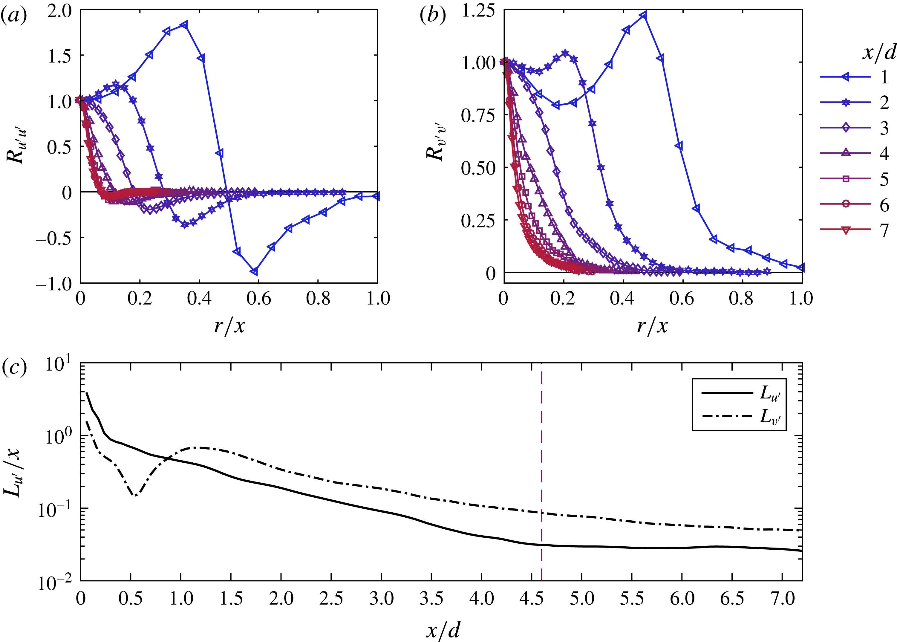
Additional insight may be obtained by considering two-point velocity correlations,
 $R_{u^{\prime }u^{\prime }}$
and
 $R_{v^{\prime }v^{\prime }}$
, taken along the jet radius originating at the centreline,
 $r=0$
(see figure 7
a,b). The onset of homogeneity may be inferred from the collapse of two-point velocity correlation functions that are normalised by the appropriate similarity variable (Davidson Reference Davidson2004). For a jet, the streamwise distance is an appropriate variable with which to normalise the correlation functions. Figures 7(a) and 7(b) show that the axial and radial velocity correlation functions, respectively, exhibit good collapse for
 $x/d>4$
, which supports the onset of homogeneity in this region. The onset of homogeneity therefore coincides with the establishment of the apparent fractal dimension
 $D=1.3{-}1.4$
(see figure 5). Evidence of homogeneity is further supported with the use of the integral length scale based on the correlation functions,
 $L_{u^{\prime }}=\int _{0}^{\infty }R_{u^{\prime }u^{\prime }}\,\text{d}r$
, plotted in figure 7(c). The length scales here are normalised by the local streamwise distance
 $x$
. The integral length scales for axial velocity fluctuations begin to plateau for
 $x/d>4$
; for the radial fluctuations the integral length scale shows signs of levelling off beyond
 $x/d\approx 5$
. Thus, the correlation functions in figure 7 demonstrate that the flow has achieved a good degree of homogeneity beyond the potential core (
 $x/d=4.6$
), which coincides with the apparent fractal dimension
 $D=1.3{-}1.4$
.
Two-point correlation functions of (a) axial velocity and (b) radial velocity along radial coordinates from the jet centreline at different
 $x/d$
locations. (c) The radial integral length scale for the axial velocity (solid line) and the radial velocity (dashed line) fluctuations. The end of the potential core in the near field is denoted by the dashed red line.

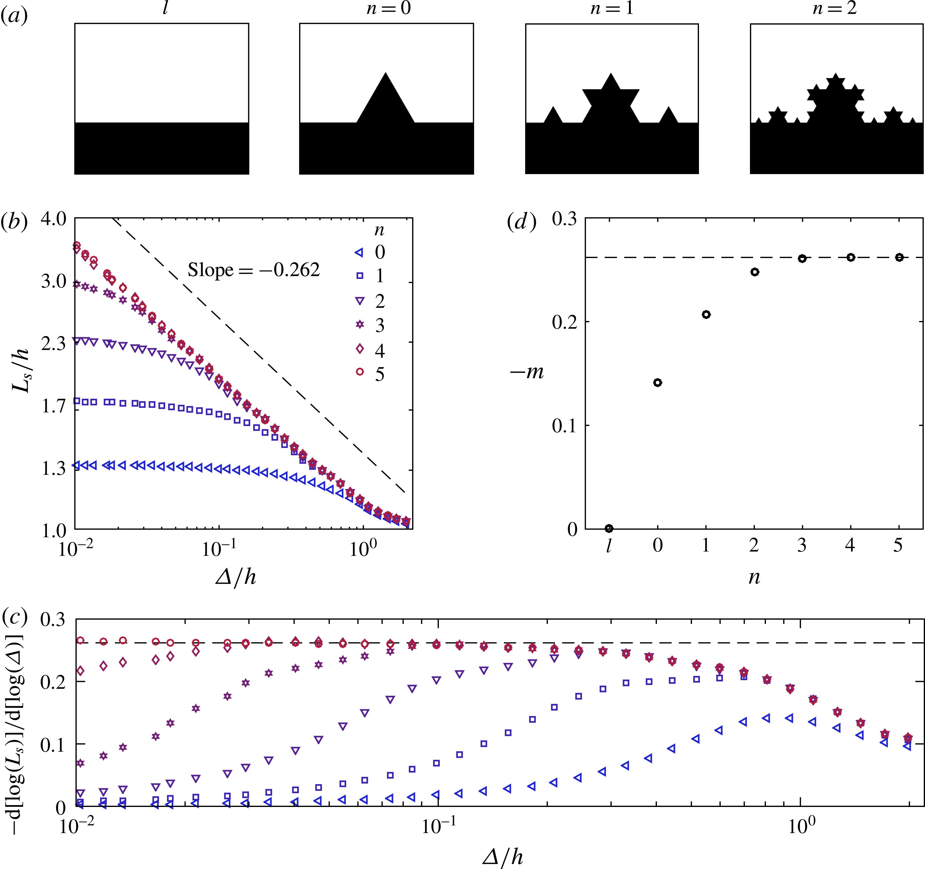
(a) Examples of discretised binary fields generated using a Koch curve to define the boundary. (b) Scaling of the Koch curve interface length
 $L_{s}$
as a function of filter size
 $\unicode[STIX]{x1D6E5}$
;
 $h$
represents the height of the triangle shape shown in panel (a) for
 $n=0$
. The black dashed line indicates the scaling of the large-
 $n$
asymptote for a Koch curve. (c) Local slope of the profiles measured in panel (b). The black dashed line indicates the scaling of the large-
 $n$
asymptote for a Koch curve. (d) Measured slope
 $m=1-D$
as a function of the number of fractal iterations
 $n$
; the featureless line profile is denoted by case
 $l$
. The dashed line indicates the asymptotic fractal dimension for a Koch curve
 $D=1.262$
.

5 Fractal construction
We now examine the region
 $x/d<4.6$
where the slope
 $m$
, and therefore the apparent fractal dimension, varies with downstream distance (see figure 5
c). Is there a physical explanation for the evolution of
 $m$
from the nozzle exit to the end of the potential core? To answer this question we investigate the multi-scale characteristics of a known fractal geometry. Here, we use the classic Koch curve as illustrated in figure 8(a).
The fractal construction is intended to be illustrative and show that the observed trends presented in figure 5 might reflect increasing scale separation. To do this, we vary the number of iterations of the fractal curve from
 $n=0$
to
 $n=5$
; with increasing iterations of pattern replication the Koch curve becomes more complex which is analogous to wrinkling of the TNTI. We begin with a featureless line profile denoted by case
 $l$
. The Koch curve is used to define the boundary in a discretised binary field which is analogous to the scalar fields shown in figure 4. The binary fields are spatially filtered in a manner similar to that described earlier in this paper. At each filter size
 $\unicode[STIX]{x1D6E5}$
we measure the length of the contour
 $L_{s}$
that is defined along points where
 $\unicode[STIX]{x1D719}=0.5$
; this represents the ‘interface’ of the synthetic field. The scaling of
 $L_{s}$
as a function of
 $\unicode[STIX]{x1D6E5}$
is shown in figure 8(b). We note that the classic box-counting technique applied to the non-discretised Koch curves recovers the asymptotic fractal dimension for this geometry (
 $D=\log (4)/\text{log}(3)$
, where
 $N\sim \unicode[STIX]{x1D6E5}^{-D}$
and
 $N$
is the box count). The box-counting fractal dimension
 $D$
is related to the coarse-grained scaling exponent by
 $D=1-m$
because
 $L_{s}\sim N\unicode[STIX]{x1D6E5}$
, where
 $L_{s}$
is the interface length measured from the spatially filtered fields. The purpose of discretising the Koch curves and spatially filtering the data is to replicate the procedure implemented on the experimentally acquired scalar data.
Similar to the process implemented in § 4 we evaluate the local slope of the Koch construction in figure 8(c),
 $m(\unicode[STIX]{x1D6E5})=-\text{d}[\log (L_{s})]/\text{d}[\log (\unicode[STIX]{x1D6E5})]$
. For
 $n=0$
the maximum slope reaches
 $-m=0.14$
, which represents the best-guess apparent fractal dimension for this geometry. Iterations
 $n=1$
and
 $n=2$
are similar in that they do not exhibit a scale-invariant slope
 $m(\unicode[STIX]{x1D6E5})$
. It is not until we reach
 $n=3$
that there is sufficient scale separation to identify a linear scaling region in figure 8(c).
The apparent fractal dimensions from these profiles are illustrated in figure 8(d), where we plot
 $-m$
for the different geometrical iterations
 $n$
; the horizontal dashed line represents the large-
 $n$
asymptote
 $D=1.262$
. The asymptotic fractal dimension is not obtained using the spatial filtering technique until a sufficient scale separation is achieved at
 $n=3$
, even though the geometry we measure in figure 8 is produced using an exact construction of a fractal curve. In this regard, the evolution of the apparent fractal dimension as a function of the iteration number
 $n$
is consistent with the development of the hierarchy of scales in turbulence as measured in the near-field region of a jet. In particular, figure 5 does not necessarily imply that the ‘true’ fractal dimension of the TNTI evolves in the development region of a jet. Rather, its apparent variation may simply reflect the effects of limited scale separation that yield an apparent fractal dimension less than the asymptotic value. The onset of an apparently asymptotic fractal dimension
 $D\approx 1.35$
therefore signifies a sufficiently developed scale separation along the TNTI, which is observed beyond the potential core region in the axisymmetric jet.
6 Conclusions
In this paper we characterise the geometric evolution of the turbulent/non-turbulent interface in the near-field region of an axisymmetric jet. Simultaneous velocity and scalar fields were obtained to investigate the scale dependence of the TNTI length by applying spatial filtering over two decades of scale separation in order to infer the apparent fractal dimension of the TNTI surface area,
 $D_{f}$
.
We show that scale invariance of the TNTI geometry is achieved at the end of the potential core at
 $x/d=4.6$
which corresponds to a fractal dimension of
 $D_{f}\approx 2.35\pm 0.02$
inferred from two-dimensional data. An equivalent fractal scaling,
 $D_{f}\approx 2.33\pm 0.01$
, of the TNTI surface area has also previously been reported in the self-similar region of the jet between
 $x/d=40{-}60$
(Mistry et al.
Reference Mistry, Philip, Dawson and Marusic2016). This means that the fractal dimension previously observed in the self-similar region of the jet is not exclusively a far-field result, as might be inferred from results to date, but rather, is a result that holds as far upstream as the end of the potential core.
The development of fractal scaling by the end of the potential core is also an indication that sufficient scale similarity of the interface geometry has been achieved. In addition, two-point velocity correlations along radial coordinates at various downstream distances show that the turbulence achieves radial homogeneity near the end of the potential core, which coincides with the onset of a measurable scale invariance of the TNTI. This lends additional support to the notion that scale similarity of the TNTI geometry is developed at this early stage.
A simple Koch construction demonstrates that a sequence of geometrical refinements that converge exactly to fractal scaling with a known value of fractal dimension exhibits a dependence of geometrical structure on scale range that is fully analogous to the streamwise dependence of TNTI geometrical structure. This supports the proposed interpretation of that dependence, and more broadly, it indicates that such considerations should apply to fractal analysis of geometrical data more generally.
Acknowledgements
The authors wish to thank the Engineering and Physical Sciences Research Council (research grant no. EP/I005897/1) and the Norwegian Research Council (project no. 244386) for the financial support of this work.