



1. Introduction
The transition around the roughness element remains an important issue, as previous investigations have shown that the transition can be accelerated significantly by the roughness (Tani & Sato Reference Tani and Sato1956; Schneider Reference Schneider2008; Zhong & Wang Reference Zhong and Wang2012). Controlling roughness element-induced transition is essential for reducing the heating flux and wall friction, thereby enabling more economical and sustainable flight. In the prediction of the transition induced by a roughness element, the roughness Reynolds number
 $\textit{Re}_h{=u_hh/v_h}$
is found to be a significant parameter, where
 $u_h$
,
 $v_h$
are respectively the streamwise velocity and kinematic viscosity at
 $y_h$
in the corresponding clean flat-plate boundary layer and
 $h$
is the roughness height (Smith & Clutter Reference Smith and Clutter1959; Van Driest & McCauley Reference Van Driest and McCauley1960). The increase in
 $\textit{Re}_h$
will change the stability character of the wake of the roughness, and a large
 $\textit{Re}_h$
can induce the absolute instability (Weingärtner et al. Reference Weingärtner, Mamidala and Fransson2023). Reda (Reference Reda2002) analyses the available experimental data of roughness-dominated transition, and the transition correlation could be well modelled by the critical roughness Reynolds number. However, many effects, including roughness pattern and inflow condition, will contribute to the inability to establish a universal
 $\textit{Re}_h$
. For example, Denissen & White (Reference Denissen and White2008) highlight that the effect of spanwise spacing on
 $\textit{Re}_h$
is not negligible. Based on direct numerical simulation (DNS) data for a smooth roughness, (Redford et al. Reference Redford, Sandham and Roberts2010),
 $\textit{Re}_h$
is found to increase as the Mach number increases and is higher for the cooled wall condition, and the findings are further confirmed by another investigation by DNS about the transition induced by the sharp-edged roughness.
A comprehensive understanding of the fundamental mechanisms underlying the roughness-induced transition is crucial for achieving accurate flow modelling and developing effective control strategies. Previous studies have demonstrated that counter-rotating streamwise vortex pairs generated downstream of the roughness element (Gaster et al. Reference Gaster, Grosch and Jackson1994; Tumin & Reshotko Reference Tumin and Reshotko2005) induce streak structures through the lift-up mechanism (Landahl Reference Landahl1975; Jacobs & Durbin Reference Jacobs and Durbin2001). Consequently, the transient growth mechanism has been proposed as a potential transition mechanism. Research on transient growth reveals that moderate to strong external perturbations are rapidly amplified at algebraic rates, forming streak structures. Within these high-amplitude streaks, nonlinear interactions between the streaks lead to secondary instability manifested as two distinct modes: sinuous and varicose, each exhibiting unique characteristics (Andersson et al. Reference Andersson, Brandt, Bottaro and Henningson2001). Tumin & Reshotko (Reference Tumin and Reshotko2001) employed optimisation methods to identify optimal instability modes for spatial stability analysis, demonstrating that steady counter-rotating vortex pairs (CRVPs) induce streaks with higher perturbation growth gains compared with those with a certain frequency. Asai et al. (Reference Asai, Minagawa and Nishioka2002) suggested that the symmetric varicose mode is influenced by Kelvin–Helmholtz instability dominated by wall-normal shear, while the antisymmetric mode is primarily governed by a wake-type instability influenced by spanwise shear. The relative dominance of these modes depends on the ratio of streak width to shear layer thickness. However, White (Reference White2002) noted quantitative discrepancies between roughness-induced instability growth and transient growth theory predictions, particularly in wall-normal disturbance profiles and streamwise locations of maximum energy growth, attributed to non-optimal perturbations generated by roughness elements. Recent research, utilising methods including global stability analysis, parabolised stability equation (De Tullio et al. Reference De Tullio, Paredes, Sandham and Theofilis2013; Cherubini et al. Reference Cherubini, De Tullio, De Palma and Pascazio2013; De Tullio & Sandham Reference De Tullio and Sandham2015; Padilla Montero & Pinna Reference Padilla Montero and Pinna2020; Ma & Mahesh Reference Ma and Mahesh2022), has focused on classifying these wake instabilities and quantifying the underlying instability mechanisms. De Tullio et al. (Reference De Tullio, Paredes, Sandham and Theofilis2013) investigated the instability of the isolated sharp-edged geometry roughness via DNS, biglobal and parabolised stability equation - three-dimensional stability in a Mach 2.5 boundary layer. The most unstable mode is identified, which is associated with varicose and sinuous deformations of the low-velocity streak resulting from instabilities in the three-dimensional (3-D) shear layer as a whole and in the lateral shear layer, respectively. These wake modes exhibited growth rates 30 times faster than those in roughness-free boundary layers. Triglobal stability analysis was performed in the wake of cylinder roughness, and the results also identify two types of global instability, i.e. sinuous instability and varicose instability (Loiseau et al. Reference Loiseau, Robinet, Cherubini and Leriche2014). Furthermore, the kinetic transfer analysis proves that the sinuous instability is related to the near-wake region of the associated reversed flow region, while the varicose mode is associated with the whole 3-D shear layer surrounding the central low-velocity streak. In their investigation of DNS transition induced by the isolated diamond-shaped trip, Shrestha & Candler (Reference Shrestha and Candler2019) identified the interaction between shear layers and counter-rotating streamwise vortices as the origin of instability downstream of the roughness. For relatively large roughness elements (e.g. those with heights exceeding the boundary layer thickness), a self-sustaining oscillatory mechanism ultimately leads to transition, as demonstrated in the investigation concerning a cylindrical roughness element in a Mach 6 boundary layer (Subbareddy et al. Reference Subbareddy, Bartkowicz and Candler2014). The self-sustaining oscillatory mechanism involves the flow structures, including the upstream shock system, horseshoe vortices and the shear layer separating from the top and sides of the roughness element. To analyse the evolution of wake modes from an energy perspective, Padilla Montero & Pinna (Reference Padilla Montero and Pinna2021) derived the temporal energy growth rate equation for two-dimensional (2-D) perturbations, incorporating the effect of entropy perturbation. They found that most of the potential energy is derived from the transport of disturbance entropy across the baseflow temperature gradients, and most of the kinetic energy is sourced from the work of the disturbance Reynolds stresses against the baseflow velocity gradient.
To delay transition induced by the discrete roughness element, many passive/active control strategies have been developed, including the introduction of additional roughness (Sharma et al. Reference Sharma, Drews, Kuester, Goldstein and White2014; Kuester & White Reference Kuester and White2015; Suryanarayanan et al. Reference Suryanarayanan, Goldstein, Berger, White and Brown2017) and the application of wall blowing/heating strip (Lu et al. Reference Lu, Zeng, Liu, Liu and Yan2021; Liu et al. Reference Liu, Huang, Tan and Liu2024), among others. Investigation based on experiment and numerical simulation confirmed that placing an anti-roughness element at a specific location downstream of the single skewed roughness element led to the effective delay of laminar–turbulent transition (Sharma et al. Reference Sharma, Drews, Kuester, Goldstein and White2014; Suryanarayanan et al. Reference Suryanarayanan, Goldstein, Berger, White and Brown2017), in which the second roughness element can suppress the high-/low-velocity streak downstream of the first one. The shielding effect, in which smaller distributed roughness can attenuate the impact of larger roughness peaks, is another passive control strategy for transition delay (Kuester et al. Reference Kuester, Sharma, White, Goldstein and Brown2014; Kuester & White Reference Kuester and White2015), and its control effect is less sensitive to roughness shape than the anti-roughness control method. A further investigation about the shielding effect clarifies the control mechanism into two parts: the upstream distributed roughness can be viewed as reducing the effective height of the discrete roughness element (DRE), and the downstream distributed roughness can reduce the streamwise vorticity (Suryanarayanan et al. Reference Suryanarayanan, Goldstein, Berger, White and Brown2020). This investigation also found that a flat roughness strip placed only upstream or only downstream of the roughness element can also effectively delay the transition. However, the control effect of the upstream roughness is limited by its height, such that a large height of the control roughness will lead to transition promotion (Lu et al. Reference Lu, Liu, Liu and Yan2020a ). Detailed DNS investigation (Lu et al. Reference Lu, Liu, Liu and Yan2020b ) reveals the control mechanism of the downstream smooth-edged roughness strip, which weakens the strongest streamwise vortices in the middle of the wake. The key to this effect lies in enhancing the dissipation of the streamwise vorticity and converting it into more stable spanwise vorticity. Moreover, they found that a smaller distance between the skewed roughness element and the roughness strip yields a superior control effect by better weakening the streamwise vortices. The control effect of shielding roughness within the airfoil boundary layer was further investigated via experiment and DNS (Justiniano et al. Reference Justiniano, Brown, White, Suryanarayanan and Goldstein2024), and it was found that a favourable pressure gradient can promote the control efficiency. For active control, Lu et al. (Reference Lu, Zeng, Liu, Liu and Yan2021, Reference Lu, Liu, Zhou and Yan2022) used a 2-D blowing strip to effectively delay the Mach 2.25 boundary layer transition induced by a smooth roughness. An upstream blowing strip delays the transition by decreasing the roughness Reynolds number, while the downstream blowing has a similar control mechanism to that of the roughness strip. Moreover, both upstream and downstream large-amplitude blowing promote transition, but their underlying mechanisms are different. The former triggers unsteady disturbances in the separation zone, while the latter is characterised by a very-low-frequency mode. A control study based on the wall heating strips indicated that the heating strip can achieve a similar control effect and have a similar control mechanism with the blowing control (Liu et al. Reference Liu, Huang, Tan and Liu2024), where the biglobal stability analyses show that heating strips have less influence on the peak growth rate of the symmetric mode, but significantly shrink its unstable region.
The focus of this study is to address the gaps in our understanding of active flow control for supersonic boundary layer transition induced by sharp-edged roughness, which inherently promotes transition more readily than smooth-edged roughness. While suction is a known effective method for effectively controlling boundary layer instability, including the Tollmien–Schlichting (T-S) wave, Görtler vortex and cross-flow instability (Pralits et al. Reference Pralits, Hanifi and Henningson2002; Messing & Kloker Reference Messing and Kloker2010; Fossà & Ricco Reference Fossà and Ricco2025), prior research has primarily focused on blowing strips over smooth-edged roughness elements, leaving the efficacy and mechanisms of suction control over wake instability largely unknown. Using DNS and biglobal stability analysis, we systematically investigate the control effects and mechanisms of both blowing and suction strips on sharp-edged roughness-induced transition. Furthermore, results indicate that the control mechanism is closely related to the spatial distribution of the blowing and suction. Inspired by this finding, we propose distributed blowing/suction configurations and find that the control effectiveness can be further enhanced. Finally, the derivation of the linearised vorticity equation is performed to gain deeper insight into the control mechanism, thereby elucidating the control mechanism of the wake modes from the perspective of the vortex dynamics.
The rest of the paper is organised as follows: in § 2, the governing equations and biglobal stability analysis are introduced first, then the vorticity transport equation is adopted for analysing the variation of vorticity in the wake region with control. Then, we derive the disturbance vorticity transport equation that is used for understanding the growth mechanism and the control mechanism of the varicose and sinuous modes. Finally, the simulation set-up, including flow conditions and blowing/suction parameters, is given. Section 3 introduces the transition mechanism induced by an isolated cubic roughness element. Then, the control effect of a blowing/suction strip on the transition as well as the wake stability is examined in § 4. In § 5, we design three distributed blowing/suction configurations, and their control effects are analysed in detail. Based on the disturbance vorticity transport equation, the growth mechanism of varicose and sinuous modes is investigated in detail in § 6. Then, the wake mode-control mechanism via blowing/suction, which has a notable control effect, is analysed in § 6.3. Finally, the major findings are summarised in § 7.
2. Numerical procedure
2.1. Governing equations
The flow in this study is governed by the 3-D compressible Navier–Stokes (N-S) equations, which are written in non-dimensional form as follows:
 \begin{align} \frac {\partial \rho }{ \partial t}+\boldsymbol{\nabla }\boldsymbol{\cdot }(\rho \boldsymbol{v})=0, \\[-12pt]\nonumber \end{align}
 \begin{align} \frac {\partial (\rho \boldsymbol{v})}{\partial t}+\boldsymbol{\nabla }\boldsymbol{\cdot }(\rho \boldsymbol{v} \boldsymbol{v}+p \boldsymbol{I}-\boldsymbol{\tau })=0 , \\[-12pt]\nonumber \end{align}
 \begin{align} \frac {\partial (\rho E)}{\partial t}+\boldsymbol{\nabla }\boldsymbol{\cdot }((\rho E+p) \boldsymbol{v}-\boldsymbol{\tau } \boldsymbol{\cdot }\boldsymbol{v}-\boldsymbol{q})=0, \end{align}
where
 $\rho$
,
 $\boldsymbol{v}$
and
 $p$
are the density, velocity vector and pressure, respectively,
 $E=p/[\rho (\gamma -1)] +\boldsymbol{v}\boldsymbol{\cdot }\boldsymbol{v}/2$
denotes the total energy and
 $\boldsymbol{I}$
is the identity matrix. The viscous stress
 $\boldsymbol{\tau }$
and heat flux vector
 $\boldsymbol{q}$
are expressed according to
 \begin{align} \begin{aligned} \boldsymbol{\tau }=\frac {\mu \textit{Ma}_{\infty }}{\operatorname {\textit{Re}}}& \left ( \boldsymbol{\nabla }\boldsymbol{v} + \boldsymbol{\nabla }{\boldsymbol{v}}^{_T} -\frac {2}{3}(\boldsymbol{\nabla }\boldsymbol{\cdot }\boldsymbol{v})\boldsymbol{I} \right )\!, \\ \boldsymbol{q}=&\frac {\mu \textit{Ma}_{\infty }}{(\gamma -1) \operatorname {\textit{Pr}} \textit{Re}}\boldsymbol{\nabla }T, \end{aligned} \end{align}
where
 $\textit{Ma}_{\infty }$
is the Mach number defined as
 $\textit{Ma}_{\infty }=u_{\infty }/a_{\infty }$
,
 $u_{\infty }$
and
 $a_{\infty }$
are the free-stream velocity and sound speed, respectively. The free-stream quantities are denoted by subscript
 $_\infty$
. The Reynolds number
 $\textit{Re}$
is defined as
 $\textit{Re}=\rho ^*_{\infty } u^*_{\infty } l^*_{\textit{ref}}/\mu ^*_{\infty }$
, in which
 $l^*_{\textit{ref}}$
is the reference length. The superscript
 $^*$
denotes dimensional variables. The Prandtl number
 $\textit{Pr}$
is set to 0.72. The dynamic molecular viscosity
 $\mu$
is approximated by Sutherland’s law
 \begin{align} \mu (T) = {T}^{3/2}\frac {T_s^*/T^*_{\infty } + 1}{T^*_s/T^*_{\infty }+T} \end{align}
where Sutherland’s constant
 $T_{s}^*=110.4 K$
. Here,
 $\rho _{\infty }^*$
,
 $c_{\infty }^*$
,
 $\rho _{\infty }^*c_{\infty }^{*2}$
and
 $T_{\infty }^*$
are employed in sequence to non-dimensionalise the density, velocity, pressure and temperature, respectively.
The in-house high-order finite-difference N-S solver, HiResX, was used to solve the discretised governing equations, which have been well validated in previous studies (e.g. Ye et al. Reference Ye, Zhang, Wan, Sun and Lu2020; Zhuang et al. Reference Zhuang, Wan, Zhang, Chang, Sun and Lu2026). To ensure numerical stability, the seventh-order alternative formulation of weighted essentially non-oscillatory scheme was employed for shock capturing and treating the inviscid fluxes (Jiang et al. Reference Jiang, Shu and Zhang2013). The viscous fluxes were discretised using an eighth-order central difference scheme. Time advancement was performed with a three-stage total variation diminishing Runge–Kutta method.
2.2. Biglobal stability analysis
The 2-D biglobal stability analysis is employed to determine the eigenmodes and corresponding spatial growth rates at various streamwise locations, based on the locally parallel baseflow assumption. The baseflow is considered dependent on the spatial coordinates
 $y$
and
 $z$
, while remaining invariant in the
 $x$
-direction. The flow variable
 $\boldsymbol{q}$
is decomposed into a steady baseflow component
 $\bar {{\boldsymbol{q}}}$
and an unsteady perturbation term
 ${\boldsymbol{q}}'$
:
 ${\boldsymbol{q}}(x,y,z,t) = \bar {{\boldsymbol{q}}}(y,z) + {\boldsymbol{q}}'(x,y,z,t)$
. Under the locally parallel flow assumption, the perturbation can be expressed as
 ${\boldsymbol{q}}'(x,y,z,t) = \tilde {{\boldsymbol{q}}}(y,z)e^{i(\alpha x - \omega t)}$
, where
 $\tilde {{\boldsymbol{q}}}$
represents the 2-D complex eigenfunction. Here,
 $\omega$
denotes the prescribed real-valued frequency, while
 $\alpha$
is the complex wavenumber to be determined. The real part of
 $\alpha$
(
 $\alpha _r$
) corresponds to the streamwise wavenumber, whereas its imaginary part (
 $\alpha _i$
) represents the spatial growth rate. A negative
 $\alpha _i$
indicates an exponentially growing mode along the streamwise direction, while a positive
 $\alpha _i$
signifies a decaying mode.
To construct the spatial framework, the linear N-S equation contains terms nonlinear in
 $\alpha$
. Therefore, the form of
 $\tilde {{\boldsymbol{q}}}$
is defined as
 $\tilde {{\boldsymbol{q}}} = [\tilde {u},\tilde {v},\tilde {w},\tilde {p},\tilde {T},\alpha \tilde {u},\alpha \tilde {v},\alpha \tilde {w},\alpha \tilde {T}]$
to transform the linear equation into a generalised eigenvalue problem
 \begin{align} \boldsymbol{A}\tilde {{\boldsymbol{q}}}=\alpha \boldsymbol{B}\tilde {{\boldsymbol{q}}}. \end{align}
The effect of the spatial discretisation scheme on the eigenvalue problem result has been investigated in previous investigations (Zhong & Tatineni Reference Zhong and Tatineni2003; Hermanns & Hernández Reference Hermanns and Hernández2008). Here, the matrices
 $\boldsymbol{A}$
and
 $\boldsymbol{B}$
are obtained using an eighth-order finite central difference scheme for spatial discretisation. Periodic boundary conditions are implemented in the spanwise direction.
2.3. Disturbance vorticity equation analysis
Vorticity transport equations are broadly utilised in fluid dynamics to investigate the fundamental mechanisms governing vorticity evolution in wake flows, and have been extensively applied in studies elucidating both transition phenomena and transition control strategies (Suryanarayanan et al. Reference Suryanarayanan, Goldstein and Brown2019; Lu et al. Reference Lu, Zeng, Liu, Liu and Yan2021). However, when the DRE height is sufficiently small, the CRVPs and streak structures in the wake do not directly induce transition. Instead, transition is predominantly initiated through the amplification of sinuous or varicose modes (i.e. secondary instabilities) within the wake flow. Given that these sinuous and varicose modes represent first-order perturbations to the wake’s basic flow state, the underlying vorticity evolution mechanisms remain insufficiently understood. To address this issue, we have systematically derived the linearised vorticity transport equations governing the evolution of these perturbation modes. In § 6, these equations will be employed to conduct a comprehensive analysis of the growth mechanisms associated with both sinuous and varicose modes, along with their corresponding transition control approaches. The derivation begins with the presentation of the complete (nonlinear) vorticity transport equations
 \begin{align} \frac {\partial \boldsymbol{\omega }}{\partial t}+(\boldsymbol{u}\boldsymbol{\cdot }\boldsymbol{\nabla })\boldsymbol{\omega }=(\boldsymbol{\omega }\boldsymbol{\cdot }\boldsymbol{\nabla })\boldsymbol{u}-\boldsymbol{\omega }(\boldsymbol{\nabla }\boldsymbol{\cdot }\boldsymbol{u})+\frac {1}{\rho ^{2}}\boldsymbol{\nabla }\rho \times \boldsymbol{\nabla }\!p+\boldsymbol{\nabla }\times \left (\frac {\boldsymbol{\nabla }\boldsymbol{\cdot }\boldsymbol{\tau }}{\rho }\right )\!. \end{align}
The term
 $\boldsymbol{\omega }=\boldsymbol{\nabla } \times \boldsymbol{u}$
. The term
 $(\omega \boldsymbol{\cdot} \boldsymbol{\nabla})\boldsymbol{u}$
represents the vortical tilting effect, where the term
 $\boldsymbol{\omega }(\boldsymbol{\nabla }\boldsymbol{\cdot }\boldsymbol{u})$
denotes the vortical expansion effect. The baroclinic effect is characterised by
 $({1}/{\rho ^{2}})\boldsymbol{\nabla }\rho \times \boldsymbol{\nabla }\!p$
, and the viscous effect is represented by
 $\boldsymbol{\nabla }\times (({\boldsymbol{\nabla }\boldsymbol{\cdot }\boldsymbol{\tau }}/{\rho }) )$
.
The derivation of the disturbance vorticity transport equation originates from the linearised N-S equations. By employing the decomposition
 $\boldsymbol{q}=\overline {\boldsymbol{q}}+\boldsymbol{q}'$
, where
 $\boldsymbol{q}$
represents the flow variables (
 $\rho$
,
 $\boldsymbol{u}$
,
 $p$
), and applying the curl operator to both sides of the linearised equations, we obtain the governing equation for vorticity perturbations. Here, we consider
 $\boldsymbol{u}=\bar {\boldsymbol{U}}+\boldsymbol{u}'$
and
 $\boldsymbol{\omega }=\bar {\boldsymbol{\omega }}+\boldsymbol{\omega }'$
(with
 $\boldsymbol{\omega }'=\boldsymbol{\nabla }\times \boldsymbol{u}'$
), and substitute these expressions into (2.7) while eliminating terms governing the mean vorticity evolution. The resulting equation is expressed as
 \begin{align} \begin{aligned} &\frac {\partial \boldsymbol{\omega }^{\prime }}{\partial t} + (\overline {\boldsymbol{U}}\boldsymbol{\cdot }\boldsymbol{\nabla })\boldsymbol{\omega }^{\prime }+ \underbrace {(\boldsymbol{u}^{\prime }\boldsymbol{\cdot }\boldsymbol{\nabla })\overline {\boldsymbol{\omega }} }_{\text{$P_d$}}=\\ & \underbrace {(\overline {\boldsymbol{\omega }}\boldsymbol{\cdot }\boldsymbol{\nabla })\boldsymbol{u}^{\prime }}_{\text{$Tv_d$}} + \underbrace {(\boldsymbol{\omega }^{\prime }\boldsymbol{\cdot }\boldsymbol{\nabla })\overline {\boldsymbol{U}}}_{\text{$Ts_d$}} - \underbrace {\left (\overline {\boldsymbol{\omega }}(\boldsymbol{\nabla }\boldsymbol{\cdot }\boldsymbol{u}^{\prime })+\boldsymbol{\omega }^{\prime }\left (\boldsymbol{\nabla }\boldsymbol{\cdot }\overline {\boldsymbol{u}}\right )\right )}_{\text{$-D_d$}} + \underbrace {\left (\frac {1}{\rho ^{2}}\boldsymbol{\nabla }\rho \times \boldsymbol{\nabla }\!p\right )^{\prime }}_{\text{$B_d$}} + \underbrace {\boldsymbol{\nabla }\times \left (\frac {\boldsymbol{\nabla }\boldsymbol{\cdot }\boldsymbol{\tau }}{\rho }\right )^{\prime }}_{\text{$V_d$}}. \end{aligned} \end{align}
The term
 $P_d$
represents the production term, describing how baseflow vorticity is transported by the perturbation velocity to generate perturbation vorticity. The term
 $T_d=Tv_d+Ts_d$
characterises the interaction between vorticity and 3-D shear effects, and is the direct mathematical representation of the corresponding term employed in previous studies (Shrestha & Candler Reference Shrestha and Candler2019; Lu et al. Reference Lu, Zeng, Liu, Liu and Yan2021). To quantitatively assess the contributions from different components of the
 $T_d$
term, we decompose it into two distinct parts:
 $Tv_d$
and
 $Ts_d$
. These terms explicitly quantify the direct contributions of baseflow vorticity strength and 3-D shear to perturbation growth (note that vorticity and shear are inherently coupled). Specifically, they elucidate the underlying mechanisms of perturbation vorticity generation through two primary processes: (i) tilting of convected baseflow vorticity and (ii) tilting of perturbation vorticity by baseflow shear. The term
 $D_d$
, captures the interaction between velocity divergence (both perturbation and baseflow) and vorticity fields (both perturbation and baseflow). The baroclinic effect is denoted by the term
 $B_d$
and viscous effects by
 $V_d$
.
In (2.8), we rewrite the material derivative of the vorticity fluctuation as
 ${\rm D}\boldsymbol{\omega }'/{\rm D}t=({\partial \boldsymbol{\omega }^{\prime }}/{\partial t})+(\overline {\boldsymbol{U}}\boldsymbol{\cdot }\boldsymbol{\nabla })\boldsymbol{\omega }^{\prime }$
. By multiplying both sides of (2.8) by the complex conjugate of
 $\omega '$
and adding the resulting equation to its conjugate counterpart, we obtain
 \begin{align} \frac {{\rm D}|\boldsymbol{\omega }'|^2}{{\rm D}t}=-\boldsymbol{\omega }^{\prime T}P_d+\boldsymbol{\omega }^{\prime T} T_d-\boldsymbol{\omega }^{\prime T} D_d-\boldsymbol{\omega }^{\prime T} B_d + \boldsymbol{\omega }^{\prime T} V_d + \text{c.c.}. \end{align}
To facilitate comparison of each term’s contribution, we integrate (2.9) in the
 $y-$
 $z$
plane. For instance, the production term is integrated as
 \begin{align} P_{{\rm d}\varGamma } = \iint 2 \textit{Re} (\boldsymbol{\omega }^{\prime T}P_d){\rm d}s, \end{align}
where the subscript
 $\varGamma$
denotes the integrated quantity. In this paper, the integration plane is the
 $y{-}z$
plane. For notational simplicity, the subscripts are generally omitted.
The top row illustrates a schematic of the computational domain along with the roughness element. The bottom row displays the control configurations: green patch indicates the strip control, while red and blue patches indicate blowing/suction distributed control, respectively.

Figure 1. Long description
Panel A: The top row shows a schematic of the computational domain. It includes a buffer region, a roughness element, and a no-slip isothermal wall. The boundary layer is marked as Ma 2.5, and the flow direction is indicated by arrows. The roughness element is positioned within the boundary layer, and the blowing/suction mechanism is shown nearby. Panel B: The bottom row displays different control configurations. The green patch indicates the strip control, while the red and blue patches indicate blowing/suction distributed control, respectively. The roughness element is depicted as a square with dimensions d by d, and h represents the height of the element.
The inlet streamwise velocity profile (a) and temperature profile (b), the dashed line is the similarity solution.

2.4. Direct numerical simulation set-up
The free-stream conditions are designed to be the same as those in the previous study (De Tullio et al. Reference De Tullio, Paredes, Sandham and Theofilis2013), with a far-field temperature
 $T_\infty ^*=273.15$
K and a Mach number of 2.5. The sketch of the computational domain is shown in figure 1. The inflow boundary condition is imposed using a profile extracted from a precursor simulation that included the leading edge. The
 $u$
and
 $T$
profiles are presented in figure 2. It can be observed that the profiles extracted from the DNS are in good agreement with the boundary layer self-similar solutions. The distance from the inflow boundary to the leading edge (
 $d_0^*$
) yields a Reynolds number of
 $\textit{Re}_0=\rho ^*_\infty U_\infty ^* d_0^*/\mu _\infty ^* = 3.5 \times 10^6$
. The reference length scale (
 $l_{\textit{ref}}^*$
) corresponds to
 $\textit{Re}=\rho ^*_\infty U^*_\infty l_{\textit{ref}}^*/\mu _\infty ^*=8000$
. Note that the subscript (
 $_{\textit{ref}}$
) refers to reference values and the superscript asterisks (
 $^*$
) denote dimensional variables. Consistent with De Tullio et al. (Reference De Tullio, Paredes, Sandham and Theofilis2013), the computational domain inlet begins at
 $x=16$
rather than
 $x=0$
. The roughness element is positioned within the region
 $x\in [50,56]$
,
 $y\in [0,0.5]$
and
 $z\in [-3,3]$
, with the width of the roughness
 $d=6$
. At
 $x=50$
, the boundary layer thickness
 $\delta _{99}=1.737$
and displacement thickness
 $\delta _\theta =0.9938$
. The roughness height
 $h=0.5$
yields
 $h/\delta _{99}=0.288$
, with a corresponding roughness Reynolds number
 $\textit{Re}_h=513.6$
. The computational domain dimensions are
 $L_x\times L_{\!y}\times L_z=166\times 16\times 20$
, discretised using 1400
 $\times$
230
 $\times$
241 grid points in the streamwise (
 $x$
), wall-normal (
 $y$
) and spanwise (
 $z$
) directions, respectively. Note that the streamwise range of the computational zone is
 $x\in [16,182]$
. The wall-normal grid follows a stretching function
 \begin{align} y=L_{\!y}\frac {\sinh (b_{\!y}\eta )}{\sinh b_{\!y}}, \end{align}
where
 $\eta$
is uniformly distributed in
 $[0,1]$
and
 $b_{\!y}=4.4227$
. Under this grid configuration, the
 $y$
-direction resolution of the roughness is set by 57 grid points. The streamwise and spanwise grid distributions follow De Tullio et al. (Reference De Tullio, Paredes, Sandham and Theofilis2013) to ensure proper resolution of roughness-induced flow features and downstream transition. Grid refinement is applied near both the roughness element and control regions. In the spanwise direction, a high-order polynomial clustering ensures accurate transition modelling, with 101 and 121 grid points resolving the roughness in the
 $x$
- and
 $z$
-directions, respectively. The grid resolution is
 $\Delta x^+_{\textit{min}}\times \Delta x^+_{w}\times \Delta z^+=7.5\times 0.9\times 6.25$
, in which the dimensionless grid size is defined as
 $\Delta x_i^+ = \sqrt {\boldsymbol{\tau }_w \rho _w} \Delta x_i / \mu _w$
, where
 $\tau _w$
is the wall shear stress,
 $\rho _w$
and
 $\mu _w$
are the density and dynamic viscosity at the wall and
 $\Delta x_i$
represents the grid size in direction
 $i$
. The value of
 $ \sqrt {\boldsymbol{\tau }_w \rho _w} / \mu _w$
is calculated at
 $z=0$
in the turbulent zone. The current grid resolution is chosen referring to previous DNS studies (Pirozzoli et al. Reference Pirozzoli, Grasso and Gatski2004; Liu et al. Reference Liu, Huang, Tan and Liu2024), enabling accurate transition prediction. The grid independence verification of the transition control is also presented in Appendix A.
The no-slip and isothermal boundary conditions are imposed at the wall, where the wall temperature
 $T_w$
is set equal to the laminar adiabatic-wall temperature
 $T_{ad}=2.05$
. The downstream and upper boundaries are treated as far-field boundary layers incorporating buffer zones for effective disturbance damping. Periodic boundary conditions are implemented in the spanwise direction. Notably, this study intentionally avoided the introduction of external disturbances to initiate transition, relying instead on the inherent numerical errors of the computation as a surrogate for free-stream disturbances. This configuration aligns with established methodologies reported in a previous study (Liu et al. Reference Liu, Huang, Tan and Liu2024).
In this study, both blowing and suction are implemented downstream of the roughness element. For the blowing/suction strip control, the boundary profile
 $v_x(x,t)$
of blowing/suction is achieved via the wall-normal velocity, following the form
 \begin{align} v_x(x,t) = A\left [\cos \frac {2\pi (x-x_{blow})}{W_x}+1\right ]\!. \end{align}
The parameter
 $W_x$
denotes the width parameter of the strip, and the blowing/suction strip is limited in the range
 $R_x=[x_{blow}-W_x, x_{blow}+W_x]$
. For the control blowing with a spanwise distribution, the profile of wall blowing/suction is defined by multiplying a strip-based distribution by an additional spanwise envelope function,
 $\varGamma (z)$
, which is based on the hyperbolic tangent (tanh) function. For the centre blowing control
 \begin{align} v_{xz}(x,z,t) = v_x(x,t)\frac {1}{2}\left [\tanh \left (5\left(\frac {z}{W_z}+1\right)\right ) +\tanh \left (5\left(-\frac {z}{W_z}+1\right) \right )\right ]\!, \end{align}
in which
 $W_z=1.5$
denotes the half-spanwise size of the control blowing. For the dual-side suction control
 \begin{align} v_{xz}(x,z,t) = v_x(x,t)\frac {1}{2}\left [2-\tanh \left (4\left(\frac {z}{W_z}+1\right)\right ) -\tanh \left (-4\left(\frac {z}{W_z}+1\right) \right )\right ]\!, \end{align}
in which
 $W_z=4$
. For the single-sided suction control
 \begin{align} v_{xz}(x,z,t) = v_x(x,t) \frac {1}{2}\left [ 1 - \tanh \left (-4\left(\frac {z}{W_z}+1\right)\right )\right ]\!, \end{align}
in which
 $W_z=4$
, and there are at least 57 grid points used to resolve the blowing/suction in the
 $x$
-direction.
The comparison of roughness with sharp edge (a) and smooth edge (b). (c) The edge comparison in the
 $z=0$
plane.

Case settings for controlling roughness-induced transition. Here,
 $R_x$
indicates the streamwise location of blowing/suction in the
 $x$
-direction,
 $R_z$
in the strip control is
 $[-l_z,l_z]$
and in the distributed control reflects the range of blowing/suction, where its amplitude satisfies
 $v(x,z,t)\gt A/2$
;
 $A$
is the amplitude in (2.12) and
 $l_z=L_z/2=10$
.

Table 1. Long description
The table presents a comparison of roughness types and their parameters for various cases. It has 32 rows and 6 columns. The columns are labeled Case, Roughness type, R subscript x, R subscript z, A, and model. The rows are labeled with different cases such as HC0, MC0, HAp1, HAp2, and so on. Each row provides specific values for R subscript x, R subscript z, A, and the model used. The table includes both sharp edged and smooth edged roughness types, with varying values for R subscript x, R subscript z, and A. The model column lists different model numbers for each case.
In addition, to evaluate the efficacy of our control strategies against a smooth roughness element, the corresponding case was set up. The element’s shape is the same as that used in our previous investigation (Lu et al. Reference Lu, Zeng, Liu, Liu and Yan2021), and its shape is defined by the function
 $y_w(x, z)$
, with
 \begin{align} \begin{aligned} y_{2d}(x) &= h \left \{ \tanh \left [ \sigma _x \left ( \frac {R_x}{2} - x \right ) \right ] + \tanh \left [ \sigma _x \left ( \frac {R_x}{2} + x \right ) \right ] \right \}\!, \\[3pt] y_w(x, z) &= y_{2d}(x) \left \{ \tanh \left [ \sigma _z \left ( \frac {R_z}{2} - z \right ) \right ] + \tanh \left [ \sigma _z \left ( \frac {R_z}{2} + z \right ) \right ] \right \}\!, \end{aligned} \end{align}
in which
 $R_x=6$
,
 $R_z=6$
,
 $h=0.5$
and
 $\sigma _x=\sigma _z=1.54$
. The width of the smooth roughness at the
 $y=h/2$
is the same as the sharp-edged roughness, and the parameter
 $\sigma _x$
or
 $\sigma _z$
reflects the degree of smoothness, where a large value means a steeper edge. The shape comparison of sharp-edged and smooth-edged roughness can be found in figure 3. Details of the control configuration for all cases are provided in table 1 in the following.
3. Sharp-edged roughness-induced transition
To establish a foundation for investigating the mechanisms of blowing/suction control, we first briefly analyse the transition mechanism induced by the sharp-edged roughness without control in case HC0. Our analysis begins with a general overview of the transition evolution and an examination of wake instability via biglobal stability analysis. To definitively identify the source of disturbances, we further analyse the flow by employing dynamic mode decomposition (DMD) and an additional DNS using flow-freezing techniques (Shrestha & Candler Reference Shrestha and Candler2019).
3.1. A general overview of transition evolution
Illustration of the flow transition downstream of the sharp-edged roughness element, including iso-surfaces of Q-criterion (
 $Q=0.02$
) coloured by streamwise velocity
 $u$
, pressure contour plotted on the centre plane (
 $z=0$
) and the wall surface, the
 $\omega _x$
contours on a subregion of the cross-section at
 $x=75$
, the streamline coloured by the wall-normal distance from the wall and the semi-transparent grey iso-surface (defined by a small negative streamwise velocity
 $u$
) depicting the recirculation zone.

The main flow structures in the transition evolution have been categorised in previous investigations (De Tullio et al. Reference De Tullio, Paredes, Sandham and Theofilis2013; Subbareddy et al. Reference Subbareddy, Bartkowicz and Candler2014), including the separation bubble, shock wave, horseshoe vortex and downstream shear/counter-rotating vortex, which are summarised in figure 4 herein. As the grey iso-surface indicates, separation bubbles form immediately upstream and downstream of the roughness element. A horseshoe vortex structure is generated in the upstream recirculation zone. Combined with the Q-criterion iso-surface, these horseshoe vortices evolve transversely, bypassing the edges of the roughness element and developing toward the wake. Here, the Q-criterion is the second invariant of the velocity gradient tensor, used to identify vortices. The definition of
 $Q$
is given by
 \begin{align} Q = -\frac {1}{2} \frac {\partial u_i}{\partial x_{\!j}} \frac {\partial u_{\!j}}{\partial x_i}. \end{align}
The attached vortex forms on the roughness element’s surface, consistent with previous observations (De Tullio et al. Reference De Tullio, Paredes, Sandham and Theofilis2013). Shock wave structures are induced upstream of the roughness element, and the CRVPs form downstream of the separation bubbles, causing the high- and low-velocity streaks further downstream via the lift-up mechanism. The parameter
 $\omega _x$
shown at the
 $x=75$
cross-section illustrates the rotation direction of these counter-rotating vortices, where the low-velocity fluid is upwashed to a higher position in the centre plane. Through downstream development, the Q-criterion iso-surfaces demonstrate that hairpin vortices undergo progressive growth and subsequent breakdown to turbulence.
The contours of Q-value (a,c,e) of mean flow field and
 $u'_{\textit{rms}}$
(b,d, f) for case HC0 at locations
 $x=70$
(a,b),
 $x=80$
(c,d) and
 $x=90$
(e, f). The grey solid curves in (a,c,e) are isolines of streamwise velocity. The vector arrows in figures (b,d, f) indicate the vector field of
 $(v,w)$
.

The spatial evolution of the counter-rotating vortex and disturbance is further examined in figure 5, which provides the Q-criterion contours of the mean flow and the root mean square (r.m.s.) of the streamwise velocity
 $u'_{\textit{rms}}$
at
 $x=70,80$
and
 $90$
. Relatively strong, CRVPs are observed near the central plane downstream of the separation zone (
 $x=70$
), while comparatively weaker horseshoe vortices develop laterally on both sides (around
 $z\approx 3$
). These CRVPs elevate low-momentum fluid, creating a 3-D high-shear region. As the flow evolves downstream, the vortices persistently bend the upper shear layer while their intensity progressively diminishes. Analysis of
 $u'_{\textit{rms}}$
reveals that initial disturbances originate at the shear layer apexes and near the horseshoe vortex region. The disturbance in the upper region rapidly amplifies downstream, becoming the dominant disturbance within the bent boundary layer, and the regions of velocity fluctuations coincide with the high-shear region. This disturbance spatial distribution aligns with prior research (Shrestha & Candler Reference Shrestha and Candler2019; Lu et al. Reference Lu, Zeng, Liu, Liu and Yan2021), suggesting that the interaction between the shear layer and the CRVPs induces significant disturbance amplification.
Pressure disturbance energy spectra results (
 $E_{pp}=\hat {p}_w \hat {p}_w^+$
) of the wake instability obtained in case HC0 at (a)
 $x=70,$
(b)
 $x=80$
and (c)
 $x=90$
with
 $y=0.9, z=0$
.

The unsteady characteristics of downstream disturbances are subsequently investigated via pressure disturbance energy spectra (De Tullio et al. Reference De Tullio, Paredes, Sandham and Theofilis2013). The pressure disturbance energy spectra (
 $E_{pp}=\hat {p}_w \hat {p}_w^+$
) are computed using the Welch method (Welch Reference Welch1967) with 21 periodograms (including a Hann window function (Harris Reference Harris1978)) from a signal comprising 30 000 uniformly sampled points over a time period of
 $T_s=135$
. The dimensionless frequency
 $F = F^* U_\infty ^*/l_{\textit{ref}}^*$
, where
 $F^*$
denotes the dimensional frequency. Note that the frequency definition is also used in the biglobal stability analysis, which ensures that the two can be directly compared. At the upstream location (
 $x=70$
), the disturbance energy is predominantly concentrated within two distinct frequency bands, approximately
 $ F\in [0.8, 1.3]$
and
 $F\in [0.4,0.8]$
, with the lower-frequency band featuring a higher amplitude. However, perturbations in the higher-frequency band undergo rapid amplification downstream, and the dominant disturbance frequency exhibits a broadband distribution centred at
 $F\approx 1.1$
.
Stability analysis results for the flow at
 $x=80$
. (a) Biglobal stability spectrum at frequency
 $F=1.1$
. (b)–(d) The
 $u$
-components of the three eigenmodes possessing the largest growth rates, identified as VCOS1 (varicose mode), SIN1 (sinuous mode) and VCOS2 (varicose mode), respectively.

3.2. Analysis of the disturbance evolution
To investigate characteristics of the eigenmodes downstream of the roughness elements that underlie the disturbance evolution, a biglobal stability analysis is performed, which is an effective transition prediction and analytical tool (De Tullio et al. Reference De Tullio, Paredes, Sandham and Theofilis2013; Padilla Montero & Pinna Reference Padilla Montero and Pinna2021). Figure 7 presents the biglobal stability analysis results for the
 $y{-}z$
cross-section at
 $x=80$
with the most unstable frequency of
 $F=1.1$
, utilising the same grid configuration as in the DNS. Two computational cases were conducted: both employing an eighth-order finite-difference discretisation scheme in the spanwise direction, while differing in the normal direction with fourth-order and eighth-order discretisations, respectively, to exclude the pseudo-eigenvalues. The eigenvalue spectrum shown in figure 7(a) reveals three unstable modes. The velocity fluctuations illustrated in figure 7(b–d) indicate that the three unstable modes are identified as varicose or sinuous modes. The phenomenon of multiple eigenvalues is similar to previous investigations (De Tullio et al. Reference De Tullio, Paredes, Sandham and Theofilis2013; Padilla Montero & Pinna Reference Padilla Montero and Pinna2020). Meanwhile, it can be observed that the distribution of eigenmodes is highly consistent with the
 $u_{\textit{rms}}'$
distribution obtained in DNS (see figure 5), being concentrated in high-shear regions. Furthermore, for the uncontrolled case, figure 8 demonstrates that the varicose mode dominates the instability at extended downstream distances. The analysis of growth rates across different frequencies and locations reveals that, while the maximum growth rate diminishes downstream, the frequency of the most unstable mode consistently remains around
 $F\approx 1.1$
. The frequency obtained from stability matches well with the DNS, indicating that the dominant transition is the varicose mode.
The dependency of growth rate of varicose and sinuous mode on the frequency at
 $x=70, 80$
and
 $90$
for case HC0 without control. The labels
 $x_1,x_2$
and
 $x_3$
in the legend denote
 $x=70, 80$
and
 $90$
, respectively. The labels ‘vcos’ and ‘sin’ in the legend denote the most unstable varicose and sinuous modes, respectively.

Given that the strongly non-parallel flow near the roughness limits the accuracy of the biglobal stability analysis, we subsequently employed DMD to analyse the disturbance characteristics in the region near the roughness (Schmid Reference Schmid2010). In the spatial range selected for DMD within a domain of
 $x\in [56,75]$
,
 $y\in [0,3]$
,
 $z\in [-10,10]$
, 750 flow snapshots with an equal time interval of
 $0.11$
are utilised. Figure 9(a) presents the obtained DMD spectrum, where most modes are distributed along the unit circle. The modes with frequency
 $F\approx 1.1$
, corresponding to the third dominant mode, are highlighted in red circles. The spatial mode distribution in both
 $z=0$
and
 $y=0.7$
planes, illustrated in figure 9(b), demonstrates that dominant modes are concentrated in high-shear regions.
The DMD analysis result for the dominant mode for case HC0. (a) The DMD spectrum for case HC0, where the red dots denote the corresponding modes of
 $F\approx 1.1$
; The mode structure of the
 $u$
-component at the vertical slice at
 $z=0$
(b) and at the horizontal slice at
 $y=0.7$
(c).

The comparison of the transition process for cases with different frozen zones. The comparison of
 $\overline {C}_{\!f}$
evolution (a) and the instantaneous
 $u$
-contour on the
 $y=0.2$
plane for cases HC0 (b), HC0-F1 (c) and HC0-F2 (d).

Figure 10. Long description
Panel A: A line graph displays the skin friction coefficient (Cf) along the x-axis for three cases: HC0, HC0-F1, and HC0-F2. The x-axis ranges from 60 to 180, and the y-axis ranges from 0 to 2 times 10^-3. The graph shows that the skin friction coefficient increases with x for all three cases, with HC0-F1 and HC0-F2 closely following the trend of HC0. Panel B: A contour plot shows the instantaneous contour on the plane for case HC0. The x-axis ranges from 40 to 180, and the z-axis ranges from -10 to 10. The color bar indicates values from 0 to 2.5. The plot shows a white rectangular region near the left side, with red and blue regions indicating areas of high and low values, respectively. Panel C: A contour plot shows the instantaneous contour on the plane for case HC0-F1. The x-axis ranges from 40 to 180, and the z-axis ranges from -10 to 10. The color bar indicates values from 0 to 2.5. The plot shows a white rectangular region near the left side, with red and blue regions indicating areas of high and low values, respectively. Panel D: A contour plot shows the instantaneous contour on the plane for case HC0-F2. The x-axis ranges from 40 to 180, and the z-axis ranges from -10 to 10. The color bar indicates values from 0 to 2.5. The plot shows a white rectangular region near the left side, with red and blue regions indicating areas of high and low values, respectively.
To further locate the origin of the disturbances amplified by the downstream shear, we employed the flow-freezing technique, by virtue of its ability to filter out the influence of disturbances from different regions. This approach enables us to exclude, for example, the unsteady perturbations induced by the feedback interaction between the upstream shock system and vortex structures (Subbareddy et al. Reference Subbareddy, Bartkowicz and Candler2014). A frozen-zone treatment is implemented in the solver, where conservative variables in the frozen region are numerically enforced using their time-averaged values. These mean quantities are pre-calculated from a prior simulation with a sampling window exceeding
 $360 l_{\textit{ref}}/c$
. Two test cases, HC0-F1 and HC0-F2, were designed with frozen zones
 $x\lt 56$
and
 $x\lt 63$
, respectively. The case HC0-F1 assesses the influence of flow structures upstream of the roughness element, while HC0-F2 additionally assesses the effect of 3-D shear layers in the immediate downstream region. Figure 10 compares the mean skin-friction coefficients
 $\bar {C}_{\!f}$
and instantaneous streamwise velocity contours at
 $y=0.2$
for different cases. Similar transition scenarios are observed across cases, indicating that the upstream flow structures have a minimal impact on the transition mechanism. The fast Fourier transform (FFT) pressure signal at locations (
 $x=70,y=0.5$
) and (
 $x=90,y=0.5$
) in cases HC0-F1 and HC0-F2 is shown in figures 11(a) and 11(b). The FFT method is employed instead of
 $E_{pp}$
to facilitate clearer comparison, as the averaging process in the Welch method may obscure certain signal details. The
 $y=0.5$
position was selected to enhance the comparative analysis of low-frequency disturbances. In case HC0-F1, the upstream disturbances (
 $x=70$
) exhibit broadband low-frequency components (
 $F \approx 0.5$
) as well as high-frequency components (
 $F \approx 1.1$
), with the latter exhibiting higher amplitude. This observation suggests that the influence of upstream flow (
 $x \lt 60$
) on downstream disturbance evolution is minimal, and the primary source of low-frequency disturbances is located downstream of the roughness element. The downstream (
 $x=90$
) frequency spectrum shows concentration around
 $F \approx 1.1$
, consistent with non-freezing conditions. Notably, the low-frequency disturbance (
 $F \approx 0.5$
) at
 $x=70$
disappears in case HC0-F2, indicating that both the source and instability region of low-frequency disturbances are primarily confined to
 $x\in [56,63]$
. The spectral distributions of downstream disturbances in cases HC0-F1 and HC0-F2 are remarkably similar, with only a marginally reduced peak amplitude around
 $F=1.1$
in HC0-F2, as illustrated in figure 11(b). This amplitude reduction results from the absence of disturbance growth within the
 $x\in [56,63]$
region, although this effect is insufficient to significantly modify the transition location.
The transition mechanism induced by the smooth-edged roughness has been introduced in detail in previous studies (Lu et al. Reference Lu, Liu, Zhou and Yan2021, Reference Lu, Zeng, Liu, Liu and Yan2022). It is similarly dominated by the varicose mode instability of the wake. The unsteadiness originating from the upstream separation zone and the shock system has a relatively minor impact on the transition location. However, compared with the sharp-edged roughness, the smooth configuration exhibits weaker CRVPs downstream of the roughness, resulting in a more delayed transition (a detailed comparison is provided in Appendix B).
The comparison of FFT result for the pressure signal at
 $x=70, y=0.5, z=0$
(a) and
 $x=90, y=0.5, z=0$
(b) for cases HC0-F1 and HC0-F2.

4. Blowing/suction strip control
In this section, we systematically investigate the influence of blowing and suction strips with varying amplitudes on the transition process triggered by sharp-edged roughness elements, employing DNS and biglobal stability analysis. The flow-freezing technique and DMD are applied to thoroughly examine instability mechanisms that remain unresolved by conventional biglobal stability analysis. Furthermore, the vorticity transport analysis of the baseflow is performed to elucidate the unexpected rapid intensification of vortical structures observed under low-amplitude suction control.
4.1. Wall blowing strip control
4.1.1. Control effect of blowing strip
The comparison of
 $\overline {C}_{\!f}$
evolutions for wall blowing strip control with the sharp-edged roughness element (a) and smooth-edged roughness element (b).

The control effects of blowing strips with varying amplitudes (HAp1 –HAp5) on transition induced by sharp-edged roughness are first examined through the time- and spanwise-averaged skin-friction coefficient (
 $\overline {C}_{\!f}$
), as presented in figure 12(a). The results demonstrate that the control effect reverses as the amplitude increases; specifically, beyond a certain amplitude threshold, the blowing strip will promote the transition. For the low-amplitude control case (HAp1), the time-averaged skin-friction coefficient (
 $\overline {C}_{\!f}$
) consistently remains below that of the uncontrolled case (HC0), with a rapid increase only initiating downstream of approximately
 $x=130$
. As the blowing amplitude increases, the transition delay effect is continuously enhanced. Specifically, the skin-friction coefficient (
 $\overline {C}_{\!f}$
) exhibits a growth trend only downstream of
 $x \approx 145$
for case HAp2 and
 $x \approx 170$
for case HAp3. When the amplitude reaches 0.04 (HAp4), the transition is completely suppressed within the computational domain. Conversely, a further increase in control amplitude (HAp5) will promote the transition. Here, the
 $\overline {C}_{\!f}$
increases rapidly starting downstream of
 $x\approx 100$
, and its magnitude exceeds that of the uncontrolled case (HC0) downstream of
 $x=140$
, indicating a quicker progression to a turbulent state. Notably, this control configuration effectively delays transition for smooth-edged roughness elements even if the control amplitude reaches
 $0.05U_\infty$
. Figure 12(b) compares the evolution of the time-averaged skin-friction coefficient (
 $\overline {C}_{\!f}$
) for cases with varying blowing control amplitudes (MAp1–MAp5) against the uncontrolled case (MC0). The results demonstrate that the transition delay is progressively enhanced as the control amplitude increases. Notably, once the amplitude reaches
 $0.02U_\infty$
(MAp2), the transition is fully suppressed within the computational domain; this effective suppression persists even as the amplitude is further increased to
 $0.05U_\infty$
.
The comparison of the control effect by blowing. The
 $u$
-contour of
 $y=0.2$
plane for cases HC0 (a), HAp1 (b), HAp2 (c), HAp3 (d), HAp4 (e) and HAp5 (f).

Figure 13. Long description
Panel A: A heat map showing the contour of a plane for case HC0. The x-axis ranges from 40 to 180, and the z-axis ranges from -10 to 10. The color scale on the right indicates values from 0 to 2.5, with blue representing lower values and red representing higher values. The heat map shows a region of high intensity near the left side, transitioning to lower intensity as it moves to the right. Panel B: A heat map showing the contour of a plane for case HAp1. The x-axis ranges from 40 to 180, and the z-axis ranges from -10 to 10. The color scale on the right indicates values from 0 to 2.5, with blue representing lower values and red representing higher values. The heat map shows a region of high intensity near the left side, transitioning to lower intensity as it moves to the right. Panel C: A heat map showing the contour of a plane for case HAp2. The x-axis ranges from 40 to 180, and the z-axis ranges from -10 to 10. The color scale on the right indicates values from 0 to 2.5, with blue representing lower values and red representing higher values. The heat map shows a region of high intensity near the left side, transitioning to lower intensity as it moves to the right. Panel D: A heat map showing the contour of a plane for case HAp3. The x-axis ranges from 40 to 180, and the z-axis ranges from -10 to 10. The color scale on the right indicates values from 0 to 2.5, with blue representing lower values and red representing higher values. The heat map shows a region of high intensity near the left side, transitioning to lower intensity as it moves to the right. Panel E: A heat map showing the contour of a plane for case HAp4. The x-axis ranges from 40 to 180, and the z-axis ranges from -10 to 10. The color scale on the right indicates values from 0 to 2.5, with blue representing lower values and red representing higher values. The heat map shows a region of high intensity near the left side, transitioning to lower intensity as it moves to the right. Panel F: A heat map showing the contour of a plane for case HAp5. The x-axis ranges from 40 to 180, and the z-axis ranges from -10 to 10. The color scale on the right indicates values from 0 to 2.5, with blue representing lower values and red representing higher values. The heat map shows a region of high intensity near the left side, transitioning to lower intensity as it moves to the right.
Figure 13 depicts the transition control effectiveness by comparing flow characteristics through velocity contours at
 $y=0.2$
. For the small blowing amplitudes (HAp1, HAp2), the spanwise spacing of downstream high-velocity streaks widens, indicating interference with the CRVPs, as illustrated in figure 13(b,c). With increasing blowing amplitude (figures 13
d), the high-velocity flow downwash is suppressed immediately downstream of the control blowing, resulting in weakened streaks. Further downstream (
 $x\gt 64$
), the downwash intensifies, generating new streaks within existing high-velocity streaks. However, when the amplitude increases to
 $0.05$
(figure 13
f), the new irregular high-velocity streaks appear at both sides of the CRVPs (
 $z\gt 3$
and
 $z\lt -3$
), making the CRVPs more unstable and breaking down further upstream, indicating that the large-amplitude blowing will introduce a new instability. Additionally, the blowing control induces an adverse pressure gradient that reduces the streamwise velocity upstream of the blowing strip, particularly evident at higher amplitudes where distinct deceleration regions form on both sides of the roughness element. In contrast, the control for the smooth-edged roughness element (figures 13
e–f) demonstrates significant streak suppression and prevents transition (MAp5) within the computational domain.
The Q-criterion contours (a,c,e) of mean flow at locations
 $x=70$
(a,d,g, j),
 $x=80$
(b,e,h,k) and
 $x=90$
(c, f,i,l) for cases HC0 (a,b,c), HAp1 (d,e, f), HAp3 (g,h,i) and HAp5 (j,k,l). The grey solid curves represent isolines of streamwise velocity, sampled at an interval of 0.2 in the range of
 $[0,2.5]$
.

The
 $u_{\textit{rms}}'$
distribution at
 $x=70$
(a,d,g,j),
 $x=80$
(b,e,h,k) and
 $x=90$
(c, f,i,l) for cases Hc0 (a,b,c), HAp1 (d,e, f), HAp3 (g,h,i) and HAp5 (j,k,l). The vector arrow indicates the vector field of
 $(v,w)$
.

Figure 15. Long description
Panel A: A heat map showing the distribution of vector fields for case Hc0 at x = 70. The x-axis ranges from -5 to 5, and the y-axis ranges from 0 to 2. The color scale indicates the magnitude of the vector field, with values ranging from 0 to 10^-3. The vector arrows indicate the direction and magnitude of the vector field. Panel B: A heat map showing the distribution of vector fields for case Hc0 at x = 80. The x-axis ranges from -5 to 5, and the y-axis ranges from 0 to 2. The color scale indicates the magnitude of the vector field, with values ranging from 0 to 4 x 10^-3. The vector arrows indicate the direction and magnitude of the vector field. Panel C: A heat map showing the distribution of vector fields for case Hc0 at x = 90. The x-axis ranges from -5 to 5, and the y-axis ranges from 0 to 2. The color scale indicates the magnitude of the vector field, with values ranging from 0 to 0.04. The vector arrows indicate the direction and magnitude of the vector field. Panel D: A heat map showing the distribution of vector fields for case HAp1 at x = 70. The x-axis ranges from -5 to 5, and the y-axis ranges from 0 to 2. The color scale indicates the magnitude of the vector field, with values ranging from 0 to 4 x 10^-4. The vector arrows indicate the direction and magnitude of the vector field. Panel E: A heat map showing the distribution of vector fields for case HAp1 at x = 80. The x-axis ranges from -5 to 5, and the y-axis ranges from 0 to 2. The color scale indicates the magnitude of the vector field, with values ranging from 0 to 1 x 10^-3. The vector arrows indicate the direction and magnitude of the vector field. Panel F: A heat map showing the distribution of vector fields for case HAp1 at x = 90. The x-axis ranges from -5 to 5, and the y-axis ranges from 0 to 2. The color scale indicates the magnitude of the vector field, with values ranging from 0 to 2 x 10^-3. The vector arrows indicate the direction and magnitude of the vector field. Panel G: A heat map showing the distribution of vector fields for case HAp3 at x = 70. The x-axis ranges from -5 to 5, and the y-axis ranges from 0 to 2. The color scale indicates the magnitude of the vector field, with values ranging from 0 to 2 x 10^-3. The vector arrows indicate the direction and magnitude of the vector field. Panel H: A heat map showing the distribution of vector fields for case HAp3 at x = 80. The x-axis ranges from -5 to 5, and the y-axis ranges from 0 to 2. The color scale indicates the magnitude of the vector field, with values ranging from 0 to 4 x 10^-3. The vector arrows indicate the direction and magnitude of the vector field. Panel I: A heat map showing the distribution of vector fields for case HAp3 at x = 90. The x-axis ranges from -5 to 5, and the y-axis ranges from 0 to 2. The color scale indicates the magnitude of the vector field, with values ranging from 0 to 0.01. The vector arrows indicate the direction and magnitude of the vector field. Panel J: A heat map showing the distribution of vector fields for case HAp5 at x = 70. The x-axis ranges from -5 to 5, and the y-axis ranges from 0 to 2. The color scale indicates the magnitude of the vector field, with values ranging from 0 to 0.1. The vector arrows indicate the direction and magnitude of the vector field. Panel K: A heat map showing the distribution of vector fields for case HAp5 at x = 80. The x-axis ranges from -5 to 5, and the y-axis ranges from 0 to 2. The color scale indicates the magnitude of the vector field, with values ranging from 0 to 0.2. The vector arrows indicate the direction and magnitude of the vector field. Panel L: A heat map showing the distribution of vector fields for case HAp5 at x = 90. The x-axis ranges from -5 to 5, and the y-axis ranges from 0 to 2. The color scale indicates the magnitude of the vector field, with values ranging from 0 to 0.2. The vector arrows indicate the direction and magnitude of the vector field.
The amplitude effect of blowing control on the flow structure and disturbance evolution is further illustrated using the
 $z{-}y$
cross-sections, as shown in figures 14 and 15. Figure 14(a) shows that, even with a small amplitude (HAp1), the blowing will significantly widen the spanwise spacing of the CRVPs and promote the intensity of the CRVP. Notably, a weaker secondary counter-rotating vortex rotating in an opposite direction is induced between the main vortices, as also evidenced in figure 15(a,d,g). As the continued induction effect of the secondary CRVPs persists, the flow at the centre plane (
 $z=0$
) is shifted from an upwash to a downwash at
 $x=90$
, while a new upwash region emerges between the two CRVPs (
 $z\approx \pm 0.7$
). Simultaneously, the wall-normal shear near the symmetry plane is weakened significantly. Despite the weaker strength of the inner CRVP, it fundamentally alters the form of the instability. As shown in figure 15(a,d,g), the disturbance near the symmetry plane is significantly suppressed, which is related to the local reduction of wall-normal shear and the weakened upwash. The disturbances are primarily distributed in the regions where their respective upwash interacts with the shear layer, and as the flow develops downstream, they evolve outwards along the rotational direction of the vortex structure, which may indicate an increased importance of spanwise shear in the mode instability.
Increasing the blowing amplitude to 0.03 (HAp3), the spatial evolution of the dual CRVPs is altered, and the nature of the disturbance instability changes simultaneously (subfigures (b,e,h) in figures 14 and 15). Firstly, the primary vortex pair is elevated to a higher position (see figure 14
b), and the secondary vortex pair exhibits enhanced intensity and an expanded spatial scale. As the flow develops downstream (figure 14
e,h), the inner CRVP weakens, while the outer CRVP descends to its original height, with its intensity continuously decreasing. The downwash at the centre plane and the upwash on both its sides are enhanced, and low-momentum fluid is lifted to a higher position. Secondly, the upstream disturbance is not directly related to the interaction between the upwash and the shear layer, as shown in figure 15(b,d). The disturbance is now concentrated at the interface of distinct vortex structures, specifically between the inner and outer CRVPs, and between the outer CRVPs and horseshoe vortices, while those two are spatially connected. The spatial variation of disturbances implies that the unsteady motion of the vortex structures is now the dominant instability mechanism. As the flow develops downstream (at
 $x=80,90$
), the disturbance at the interface between the outer vortex and the horseshoe vortex is observed to be relatively weak, whereas the disturbance at the interface between the inner and outer vortices intensifies and dominates the development of instability. It can be hypothesised that the weakening of the former disturbance is likely due to the viscous dissipation of the outer horseshoe vortex, which is seen to weaken further downstream, as illustrated in figure 14(b,e,h) (the horseshoe vortex is located near
 $z=\pm 3, y\approx 0.4$
).
When the blowing amplitude is increased to 0.05 (HAp5), the original CRVPs are observed to be positioned higher and have a wider spanwise spacing. Furthermore, more secondary vortex pairs are present in the central region (as also observed in figure 15
c,f,i). As the flow develops downstream, both the primary and secondary vortices weaken. The upwash motion is predominantly observed at the central symmetry plane and on the inner side of the primary vortices (
 $z \approx \pm 1.5$
). Notably, the outer side of the horseshoe vortex (
 $z\approx \pm 3$
) also appears to induce a new vortex structure (
 $z\approx \pm 4.8$
), with a relatively clear upwash process forming between the horseshoe vortex and this newly induced structure (
 $z\approx \pm 4$
). The disturbance distribution becomes more complex, but it can be roughly categorised into two types of regions. The first type lies along the interfaces of the vortices, specifically between the primary CRVPs and the secondary CRVPs. The second type is located closer to the core of the vortex structures, primarily corresponding to the location of the horseshoe vortices and their secondary vortices. It can be hypothesised that both types of disturbance originate from the motion of the vortices and mutually interact with each other. However, their fundamental sources of instability are not entirely identical: the former arises from the evolution of the original CRVP disturbance, while the latter is attributed to the horseshoe vortex and its secondary structures. Figure 13(d) further confirms this by showing the appearance of irregular and unstable high- and low-velocity streaks immediately downstream of the blowing strip.
The disturbance frequency spectra of the pressure for the blowing control cases HAp1 (a,d), HAp3 (b,e) and HAp5 (c,f). The monitor locations are detailed in the legend using
 $(x, y, z)$
coordinates. The figures in the upper and lower rows present results at the streamwise positions
 $x=70$
and
 $x=80$
, respectively. The results for cases HAp1 and HAp3 were obtained using FFT, while the power spectrum analysis was applied to case HAp5.

The disturbance frequency spectra at the monitor points in figure 16 further characterise the features of instability evolution and can be used to distinguish between different instability mechanisms. The monitor points are located within the two planes at
 $x=70$
and
 $x=80$
, with the specific location dependent on the region where the disturbance is present. It reveals that the small blowing amplitude (HAp1) shifts the upstream dominant frequency to a broadband peak at
 $F=1.5$
, which is higher than the uncontrolled case (HC0). Then the dominant frequency shifts to
 $F\approx 1.1$
downstream, which is close to that without control. Figures 16(b) and 16(e) present the disturbance spectra for case HAp3. The monitor points at
 $(70, 0.7, 1.5)$
and
 $(80, 0.9, 1)$
reflect the disturbance at the interface between the original CRVPs and the secondary CRVPs. In contrast, the monitor points at
 $(70, 0.7, 3)$
and
 $(80, 0.5, 3)$
capture the disturbance at the interface between the original CRVPs and the horseshoe vortices. Analysis of the streamwise spectral evolution reveals that the instability frequency band of the latter (CRVPs/horseshoe interface) is primarily centred around
 $F=0.9$
. For the former (CRVPs/secondary CRVPs’ interface), the instability frequency is concentrated around
 $F=0.7$
upstream and decays to approximately
 $F=0.5$
downstream. It is notable that the spectra of these two sets of monitor points exhibit some overlap. This suggests that the spatial regions of the two distinct instabilities may be interacting or spatially overlapping. Figures 16(c) and 16(f) display the disturbance spectra for case HAp5. The monitor points at
 $(70, 0.7, 1.5)$
and
 $(80, 0.7, 1.5)$
reflect the disturbance at the vortex interfaces, while those at
 $(70, 0.3, 3)$
and
 $(80, 0.5, 3)$
capture the disturbance near the horseshoe vortices. Evidently, the unsteady motion of the horseshoe vortex exhibits a very low-frequency characteristic, approaching
 $F\approx 0.1$
, and dominates the evolution of the instability in the
 $y{-}z$
plane upstream. Further downstream, the disturbance near the horseshoe vortex grows slowly, but the disturbance at the vortex interfaces grows more rapidly and is centred around a frequency of
 $F=0.9$
. The difference in dominant frequencies further suggests that the instability mechanisms are distinct.
The comparison of the most unstable mode obtained via biglobal analysis for cases HAp1 (a), HAp3 (b), HAp5 (c). The labels
 $x_1,x_2$
and
 $x_3$
in the legend denote
 $x=70, 80$
and
 $90$
respectively. The labels ‘vcos’ and ‘sin’ denote the most unstable varicose and sinuous mode, respectively. The red solid/blue line indicates the most unstable varicose mode for case HC0 and cases with blowing control, and the blue dashed line indicates the most unstable sinuous mode for cases with blowing control.

4.1.2. Control mechanism of blowing strip
To further reveal the effect of the blowing strip on the instability in the roughness wake, biglobal stability analysis is utilised, and the growth rates of varicose and sinuous modes at different locations are provided in figure 17. The baseflow for the biglobal stability analysis is obtained by time averaging the flow field over a period of
 $T_s=135$
. Since the disturbances remain small in the region
 $x \leqslant 90$
, the baseflow is not affected by nonlinear effects in this area. The numerical setting for the biglobal stability analysis is the same as that used in case HC0. It can be found that, for all control amplitudes, the growth rates of the most unstable mode for all blowing control cases are lower than that of HC0 for all positions. Furthermore, the varicose mode is suppressed to a greater extent compared with the sinuous mode, and in the case of HAp1, the sinuous mode is even promoted at the upstream location (
 $x=70$
). Hence, the sinuous mode becomes the dominant mode in the wake for a distance downstream with blowing control, indicating the motion of vortex pairs on each side of the symmetry plane is anti-phase. Furthermore, it can be observed that the control effectiveness is not monotonic with respect to the control amplitude; the maximum suppression of both the varicose and sinuous modes occurs in the HAp3 case. The frequency of the most unstable mode also shifted with control, which showed good agreement with the results from DNS at most positions (figure 16). Note that the slight discrepancy of frequency spectra at
 $x=80$
in the HAp5 case might be caused by the slightly stronger flow non-parallelism.
The flow evolution for case HAp5-F1, which incorporates the flow-frozen technique with the frozen range of
 $x\lt 56$
applied to the HAp5 configuration. The streamwise velocity contour on the
 $y=0.2$
plane (a); the dark shaded area indicates the range of the flow-frozen region. The frequency spectrum for the monitor points in the
 $x=70$
(b) and
 $x=80$
(c) planes. The legend depicts the coordinates
 $(x, y, z)$
of the monitor points.

Biglobal stability analysis suggests that blowing control at all three amplitudes suppresses the wake disturbance, but the DNS results reveal that higher blowing amplitudes promote transition. A possible reason for this discrepancy is that the pressure gradient caused by the blowing strip significantly promotes upstream disturbances, as previous studies reveal that the adverse pressure gradient is a key factor in disturbance growth. To validate this hypothesis, we designed the computational cases (HAp5-F1) with frozen flow regions upstream of
 $x=56$
. The flow evolution for HAp5-F1 is illustrated by the streamwise velocity on the
 $y=0.2$
plane in figure 18(a). Without the upstream disturbance, the flow field for the HAp5-F1 case shows that the irregular high- and low-velocity streaks on both sides of the CRVPs disappear, instead exhibiting a strengthened horseshoe vortex. More importantly, the transition is significantly suppressed, and specifically, the disturbance appears downstream of
 $x=170$
, indicating a weaker transition delay effect than HAp3 (compared with figure 13
c), which is consistent with the stability analysis prediction. Crucially, the control effects observed in HAp5-F1 indicate that the promoted disturbance in the region
 $x\lt 56$
is the key factor that induces the very-low-frequency unstable disturbance on both sides of the CRVPs and promotes the transition. To more rigorously validate this hypothesis, we compare the pressure frequency spectrum at the monitoring points in case HAp5 with that of HAp5-F1. The spectra from the monitor points located at
 $x=70$
and
 $x=80$
in figure 18(b,c) show that, with the introduction of the frozen flow region, the very-low-frequency disturbance disappears. The remaining disturbance frequencies are primarily concentrated around
 $F=0.5$
and
 $F=0.9$
, with the disturbance near
 $F=0.9$
exhibiting a larger growth rate. The dominant frequency of
 $F=0.9$
aligns with the stability analysis predictions and matches the instability frequency observed downstream in the baseline HAp5 case. The
 $F=0.5$
frequency, on the other hand, likely corresponds to the instability frequency identified in § 3. In short, the large blowing control leads to an amplification of the upstream low-frequency unstable disturbance, which, in turn, imparts stronger unsteady motion to the horseshoe vortex. This strengthens the instability mode related to the interaction between the horseshoe vortex and the CRVPs. Although the growth rate of the mode (with frequency
 $F\approx 0.1$
) is comparatively low, it still causes the flow to break down over a short distance, thereby significantly promoting the overall transition process.
In the comparative case involving the smooth-edged roughness element, large-amplitude blowing was observed to still significantly delay transition, which is consistent with previous investigations (Lu et al. Reference Lu, Zeng, Liu, Liu and Yan2021). This agreement can be attributed to the similar configurations of the roughness geometry and control parameters employed in both investigations. Specifically, the roughness height (
 $h/\delta _{99}$
) was comparable (0.286 in the previous study and 0.288 in the present study), as was the blowing mass flux
 $\rho _w v_w$
(0.02 and 0.04 in the prior work, versus 0.025 in the current investigation, where the wall density
 $\rho _w \approx 0.5$
). In the smooth-edged roughness, the critical amplitude that reverses the transition control effect is
 $\rho _w v_w\approx 0.23$
, which is far larger than that in sharp-edged roughness. Analysis of the results reveals that blowing similarly induces a new pair of counter-rotating vortices downstream of the smooth-edged roughness element, while the relative position between the induced vortices and the original counter-rotating pair changes less significantly in the streamwise direction. It appears that the smooth-edged roughness element is comparatively easier to control. This may be attributed to the fact that the shear and vorticity on both sides of the roughness are weaker and thus less affected by the blowing strip.
4.2. Wall suction strip control
4.2.1. Control effect of suction strip
The control effect of suction strips at different amplitudes on transition is first examined by
 $\overline {C}_{\!f}$
, as shown in figure 19(a). Interestingly, the trend in transition delay with suction amplitude is the opposite of that for blowing amplitude: small suction amplitudes (HAm1–HAm3) significantly promote transition, while a large amplitude (HAm4, HAm5) significantly suppresses it. Figure 20 illustrates this with streamwise velocity contours. In case HAm1, short and symmetrically distributed high-velocity streak structures form within the original streaks and rapidly amplify, leading to transition promotion. As the amplitude increases (HAm2, HAm3), the unstable disturbance appears earlier and loses symmetry. However, a further amplitude increase (HAm4, HAm5) significantly suppresses these disturbances, so that only simple high- and low-velocity streaks appear downstream. Furthermore, the effects of suction control on smooth-edged roughness elements were investigated. As illustrated in figure 19(b), the control laws are consistent with those observed for sharp-edged roughness elements; specifically, low-amplitude suction promotes transition, while high-amplitude suction suppresses it. The primary difference lies in the lower critical amplitude for smooth-edged elements, where transition suppression is achieved once the amplitude exceeds
 $0.02U_\infty$
. The spatial evolution at
 $y = 0.2$
plane for the smooth-edged case is provided in Appendix B, offering a more intuitive observation of a rapid reversal in the transition control effect.
Control effect by suction presented via the
 $\overline {C}_{\!f}$
for sharp-edged roughness (a) and smooth-edged roughness (b).

Control effect by suction presented via the instantaneous
 $u$
-contour at
 $y=0.2$
plane for cases HC0 (a), HAm1 (b), HAm2 (c), HAm3 (d), HAm4 (e) and HAm5 (f).

Figures 21 and 22 further illustrate the downstream flow structures and shear characteristics with suction control. In case HAm1, low-amplitude (
 $0.01U_\infty$
) suction induces a large number of vortex structures that are symmetric about
 $z=0$
. On a single side, there are at least four vortex structures rotating in different directions, resulting in a complex pattern of upwash and downwash in space. Specifically, the higher region features a strong CRVP, which causes a local upwash of the flow near the symmetry plane at that height. As the flow develops downstream, the number of vortex structures remains constant, but the vortex cores are mainly distributed near the wall and at higher locations. The arrangement of numerous vortices closely together appears to be unstable; as shown by the r.m.s. distribution (
 $u'_{\textit{rms}}$
), strong disturbances emerge upstream, concentrated at the vortex–vortex interfaces. As the flow develops further downstream, these disturbances gradually expand, corresponding to the transition. Upon increasing the suction amplitude, the number of vortex cores marked by the Q-criterion remains high, but the symmetry is broken. However, when combined with the streamline contours, it can be seen that the dominant upstream flow structure consists of a CRVP, causing the central flow to upwash. Downstream, the number of vortex pairs increases, yet the central flow consistently remains upwashed. The disturbance distribution shows strong concentration both during the flow upwash phase and at the vortex cores located in the higher regions. Further downstream, the disturbance strengthens near the centre and rapidly expands toward the wall, leading to a quick transition. However, with a further increase in suction amplitude (
 $0.05U_\infty$
), the flow structure becomes simpler. Only a single pair of counter-rotating vortices exists near the central plane. Compared with the uncontrolled case, the spanwise distance between these vortices is significantly reduced, and the upwash region becomes smaller. As the flow develops downstream, the vortex structure gradually decays. Furthermore, it can be observed that the r.m.s. distribution
 $u'_{\textit{rms}}$
is closer to that of a varicose mode, and its intensity is much lower than under lower control amplitudes.
The contour of Q-criterion of mean flow field at locations
 $x=70$
(a,d,g, j),
 $x=80$
(b,e,h,k) and
 $x=90$
(c, f,i,l) for cases Hc0 (a,b,c), HAm1 (d,e, f), HAm3 (g,h,i) and HAm5 (j,k,l). The grey solid curves are isolines of streamwise velocity.

The
 $u_{\textit{rms}}'$
distribution at locations
 $x=70$
(a,d,g, j),
 $x=80$
(b,e,h,k) and
 $x=90$
(c, f,i,l) for cases Hc0 (a,b,c), HAm1 (d,e, f), HAm3 (g,h,i) and HAm5 (j,k,l). The white vector arrow indicates the vector field of
 $(v,w)$
.

The mechanism analysis of the generation of vortex in cases HAm1 (a), HAm3 (b) and HAm5 (c) via vorticity transport term. The contours of vorticity transport terms
 $P_x$
,
 $Pxx$
,
 $Pyx$
,
 $\textit{Pzx}$
,
 $Vx$
are shown in rows 1–5, respectively.

4.2.2. Control mechanism of suction strip
The rapid proliferation in the number of vortex structures appears to be an unfavourable factor for flow stability. To understand the underlying mechanism of the vorticity generation, particularly the CRVP observed at higher height under small-amplitude suction, we conducted an analysis based on the transport equation of enstrophy
 $\omega _i^2/2$
. Following the derivation approach presented by Brown et al. (Reference Brown, Lee and Moser2015) and Suryanarayanan et al. (Reference Suryanarayanan, Goldstein, Berger, White and Brown2020), this governing equation is obtained by multiplying each component of the vorticity transport equation (2.7) by its respective vorticity component,
 $\omega _i$
 \begin{align} \begin{aligned} &\frac {\partial }{\partial t}\left(\frac {1}{2}\omega _i^2\right)+\boldsymbol{u}\boldsymbol{\cdot }\boldsymbol{\nabla }\left(\frac {1}{2}\omega _i^2\right)=\\ &\omega _i(\boldsymbol{\omega }\boldsymbol{\cdot }\boldsymbol{\nabla })u_i-\omega _i\omega _i(\boldsymbol{\nabla }\boldsymbol{\cdot }\boldsymbol{u})+ \epsilon _{ijk} \omega _i\frac {1}{\rho ^{2}}\frac {\partial \rho }{\partial x_{\!j}} \frac {\partial p}{\partial x_k} + \epsilon _{ijk} \frac {\partial }{\partial x_{\!j}} \frac {1}{\rho }\left (\frac {\partial \tau _{km}} {\partial x_m}\right )\!. \end{aligned} \end{align}
The label
 $\epsilon$
denotes the Levi-Civita symbol. The term
 $P_i=\omega _i(\boldsymbol{\omega }\boldsymbol{\cdot }\boldsymbol{\nabla })u_i-\omega _i\omega _i (\boldsymbol{\nabla }\boldsymbol{\cdot }\boldsymbol{u})$
is named production term, its component
 $P_{ii}= \omega _i^2 \partial u_i/\partial x_i$
represents the stretch of
 $\omega _i$
while
 $P_{ij}=\omega _i\omega _{\!j} \partial u_i /\partial x_{\!j}$
indicates the generation of
 $\omega _i$
via tilting mechanisms of
 $\omega _{\!j}$
. The term
 $D_i=-\omega _i\omega _i(\boldsymbol{\nabla }\boldsymbol{\cdot }\boldsymbol{u})$
is named the divergence term. The baroclinic term is
 $B=\epsilon _{ijk} \omega _i ({1}/{\rho ^{2}}) ({\partial \rho }/{\partial x_{\!j}}) ({\partial \rho }/{\partial p_k})$
and the viscous term is
 $V=\epsilon _{ijk} ({\partial }/{\partial x_{\!j}}) ({1}/{\rho }) (({\partial \tau _{km}}/ {\partial x_m}) )$
.
The individual terms of (4.1) are calculated from the mean flow averaged over the time period
 $900l_{\textit{ref}}/c$
. Since the downstream flow for cases HAm1 and HAm3 undergoes a rapid transition, which would introduce significant errors into (4.1), our analysis is confined to a limited streamwise domain (
 $x \in [56,70]$
). As terms
 $D$
and
 $B$
are statistically weak, they are not presented in figure 23. For the HAm1 case, it is evident from figure 23(a) that the
 $P_x$
term plays a critical role in the strong vorticity. For the vorticity near
 $y=1.2$
, the primary generation mechanism is the tilting of the wall-normal vorticity component, while the stretching of streamwise vorticity and the tilting of spanwise vorticity inhibit the streamwise vorticity growth. For the vorticity near
 $y=0.6$
, the streamwise stretching term becomes a significant source. The tilting of the spanwise vorticity and the wall-normal vorticity play promoting and inhibitory roles, respectively, and exhibit similar spatial distributions. Note that the term
 $\partial u/\partial z \partial u/\partial y$
is the component of
 $\omega _{\!y} \partial u/\partial y$
and the term
 $-\partial u/\partial z \partial u/\partial y$
is the component of
 $\omega _z \partial u/\partial z$
, which lead to a similar spatial distribution but roughly opposite effect of
 $P_{yx}$
and
 $P_{zx}$
.
In the HAm3 case, the near-wall flow acceleration, induced by suction, significantly promotes the stretching of streamwise vorticity. Under the influence of shear, the normal and spanwise vorticity components promote and inhibit, respectively, the streamwise vorticity at different heights, but the total effect is all promoting the streamwise vorticity. When the suction amplitude is further increased (HAm5), it can be observed that the effect of stretching and tilting is similar to that in HAm3, with the slight difference being that the near-wall vortex stretch effect is dampened.
The spectra
 $E_{pp}$
for pressure at
 $x=70$
(a,b,c),
 $x=75$
(d,e, f) and
 $x=80$
(g,h,i) for the suction control in cases HAm1 (a,d,g), HAm3 (b,e,h), HAm5 (c, f,i). The monitor points are located at
 $y=0.9$
and
 $z=0$
.

The unsteady characteristics of the instability suggest the presence of distinct instability mechanisms under suction control, a hypothesis that is further substantiated by the spectral results. Figure 24 shows the pressure spectra at different monitor points in the wake. Specifically, we found that a new ultra-low-frequency dominant mode emerges upstream in case HAm1, as shown in figure 24(a), whose frequency is
 $F\approx 0.045$
, which is approximately
 $1/24$
th of the original unstable frequency. The harmonic mode with frequency
 $F\approx 0.1$
then emerges as the most unstable disturbance and finally leads to the final transition (figure 24
d,g). The unstable ultra-low-frequency mode is also induced when the suction amplitude increases to
 $0.03U_\infty$
(HAm3). However, the broadband unstable mode centred at approximately
 $F=1.1$
is amplified, and subsequently leads to the breakdown along with the ultra-low-frequency mode. The unstable ultra-low-frequency mode disappears when the suction control increases to
 $0.05U_\infty$
(HAm5), in which the unstable frequency is similar to that of the uncontrolled case, appearing as a broadband mode around
 $F=1.5$
. The disturbance grows slowly, and its peak frequency shifts slightly toward the lower frequency.
The DMD spectrum and mode for case HAm1, (a) the spectrum distribution, (b) the energy ranking and slices of the mode with frequency
 $F\approx 0.04$
at
 $x=60$
(c) and
 $x=70$
(d). The background of (c) and (d) is the contour of the streamwise velocity, and the black line is integrated from the
 $v{-}w$
vector field of the DMD mode.

To better understand the dynamic evolution of the ultra-low-frequency mode, DMD was performed on the flow disturbances within the region defined by
 $x\in [56,70]$
,
 $y\in [0,3]$
and
 $z\in [-10,10]$
. A total of 600 instantaneous 3-D flow fields, each containing velocity components
 $(u,v,w)$
, were sampled at equal time intervals of
 $\Delta t$
for the DMD analysis. The resulting DMD modes are presented in figure 25. As shown in figures 25(a) and 25(b), apart from the first two modes corresponding to zero frequency, which represent the baseflow and a decaying mode, respectively, the most energetic mode exhibits a frequency of
 $F\approx 0.04$
, which is in good agreement with the DNS results. Figures 25(c) and 25(d) illustrate the disturbance structures in the
 $y$
–
 $z$
plane at
 $x=60$
and
 $x=70$
, respectively. The upstream disturbance is primarily characterised by a pair of counter-rotating vortices located at a higher position (
 $y=0.7$
). As the flow develops downstream, this vortex pair expands to span the entire boundary layer thickness – a behaviour markedly distinct from wake modes that typically oscillate near the boundary layer edge. This observed disturbance pattern indicates a global wandering motion of the wake vortex system. The presence of ultra-low-frequency dynamics and streamwise vortices represents a classical signature of non-modal disturbance growth within the boundary layer, consistent with the so-called lift-up mechanism. The high-gain nature of this mechanism allows disturbances to grow rapidly, thus promoting the transition to turbulence.
The ultra-low-frequency mode is completely suppressed in case HAm5, which coincides with a significant delay in transition. To analyse the underlying mechanism responsible for this transition suppression, a 2-D biglobal stability analysis was employed, as seen in figure 26. The results demonstrate that both the varicose and sinuous modes are significantly suppressed. A notable evolutionary characteristic is the shift of the most unstable mode from varicose to sinuous as the flow develops downstream. Furthermore, the most unstable frequency shifts from a high value to a low value, a finding that aligns well with the DNS results in figure 24(c).
5. Transition delay via the distributed blowing/suction configuration
The analysis of the control mechanisms associated with the blowing/suction strip inspired us to explore distributed blowing/suction for achieving superior control efficiency and effectiveness. This distributed approach allows us to circumvent two major adverse effects: the unsteadiness induced in the horseshoe vortices by the blowing strip on the sides of the roughness element, and the promotion of
 $\omega _x$
near the centre plane by the suction strip. Simultaneously, distributed blowing/suction is also expected to mitigate the drawback of local high skin friction associated with the effective strip control strategy (HAm5). Consequently, we proceeded to design three distinct configurations of distributed blowing/suction. The first configuration employs blowing at the centre downstream of the roughness element, denoted as case HBc. The second configuration involves suction on both sides downstream of the roughness element, denoted as case HSbs. The third configuration features suction on a single side, denoted as case HSss. The sketch and detail of the control can be found in figure 1 and table 1.
The comparison of the most unstable mode obtained via the biglobal analysis for cases HC0 and HAm5. The labels
 $x_1,x_2$
and
 $x_3$
in the legend denote
 $x=70, 80$
and
 $90$
, respectively. The labels ‘vcos’ and ‘sin’ denote the most unstable varicose and sinuous mode, respectively. The red solid/blue line indicates the most unstable varicose mode for case HC0 and cases with suction control, and the blue dashed line indicates the most unstable sinuous mode for cases with suction control.

Control effect by distributed control checked via the
 $\overline {C}_{\!f}$
(a) and instantaneous
 $u$
-contour at
 $y=0.2$
plane for cases HBc (b), HSbs (c) and HSss (d).

The control effect of the distributed blowing/suction on the transition induced by smooth-edged roughness: MBc (a), MSbs (b) and MSss (c).

The control effects of the three configurations of distributed blowing/suction controls are demonstrated in figure 27. The
 $\overline {C}_{\!f}$
evolutions in figure 27(a) indicate that all three control configurations can effectively delay the transition. Among them, the transitions are all delayed significantly in cases HBc and HSbs, as their
 $\overline {C}_{\!f}$
remains suppressed downstream in the whole computation zone. Case HSss provides the weaker control performance. The velocity contours in figure 27(b,c,d) indicate that the distribution of high- and low-velocity streaks downstream of the blowing/suction regions is similar to the uncontrolled case for all control configurations. A key difference is that the spanwise spacing of the high-velocity streaks is widened for a certain distance downstream of the control region in cases HBc and HSbs. In the case of HSss, it is evident that the high-velocity streaks shift towards the suction side, while the perturbation amplitude is larger on the opposite side during the early stage of transition downstream.
To validate the universality of the distributed blowing/suction control configuration, we implemented identical control strategies for transition induced by a smooth-edged roughness element, with the corresponding cases designated as MBc, MSbs and MSss, respectively. The transition control outcomes, as illustrated in figure 28, reveal that all three control strategies significantly delay the transition, demonstrating considerable universality across diverse transition scenarios. Notably, comparative analysis with sharp-edged roughness control reveals a subtle distinction: central blowing exhibits optimal performance, followed by dual-side suction as the secondary effective approach.
The evolution of the CRVP and disturbance with the three configurations of distributed blowing/suction control is further illustrated in figures 29 and 30. In the HBc case, centre blowing significantly expands the spanwise spacing of the original CRVP, and the wall-normal shear is substantially attenuated (figure 29
a,d,g). Furthermore, unlike the blowing-and-suction strip control, it does not induce a secondary vortex at the centre. The spanwise spacing of the vortices contracts further downstream, but the vortex strength changes slowly. The disturbance is primarily distributed in two distinct regions: one near the plane of symmetry (
 $y\approx 1$
), and the other concentrated within the vortex regions (figure 30
a,d,g). This suggests the coexistence of two potential instability mechanisms: one associated with the upwash–shear layer interaction, and the other related to the vortex motion. Under dual-sided suction control, the primary flow structure remains the CRVP (figure 29
b,e,h), and its strength is also significantly suppressed, with the spanwise separation of the vortex cores being substantially widened. These effects collectively lead to weakened upwash and wall-normal shear. Furthermore, as the flow evolves, the CRVP strength diminishes, and the spanwise distance between the cores also decreases. Although both cases are CRVP dominated, the instability characteristics under HSbs control are still significantly different from those under HBc control, as shown in figure 30(b,e,h). The downstream amplification of strong perturbations both along (
 $z\approx 0$
) and adjacent to the symmetry plane (
 $z\approx \pm 1$
) strongly suggests the coexistence of different instability mechanisms, both of which are inferred to be directly linked to the local flow upwash.
The wake downstream of the roughness in the single-sided suction control is still dominated by a CRVP, as shown in figure 29(c, f,i), but whose symmetry is broken, with a weakened/strengthened vortex on the suction/no-control side, leading to shear relaxation on the suction side. The vortex gradually weakens downstream, yet continuously bends the boundary layer. Moreover, the perturbation evolution indicates that the most unstable disturbance is predominantly localised within the upwash/shear layer interaction region, with a clear bias towards the suction side, implying that the instability mode corresponds to a modified varicose mode (figure 30 c, f,i).
The contours of Q-criterion (a,c,e) of average flow field at locations
 $x=70$
(a,d,g, j),
 $x=80$
(b,e,h,k) and
 $x=90$
(c, f,i,l) for cases HC0 (a,b,c), HBc (d,e, f), HSbs (g,h,i) and HSss (j,k,l). The grey solid curves are isolines of streamwise velocity.

The
 $u_{\textit{rms}}'$
distributions at locations
 $x=70$
(a,d,g, j),
 $x=80$
(b,e,h,k) and
 $x=90$
(c, f,i,l) for cases HC0 (a,b,c), HBc (d,e, f), HSbs (g,h,i) and HSss (j,k,l). The white vector arrow indicates the vector field of
 $(v,w)$
.

The mechanism analysis of generation of the vortex in cases HBc (a), HSbs (b) and HSss (c) via the vorticity transport term. The contours of vorticity transport terms
 $P_x$
,
 $P_{xx}$
,
 $P_{yx}$
,
 $P_{zx}$
,
 $V_x$
are shown in rows 1–5 respectively.

To understand the vorticity variation mechanism under the distributed blowing/suction control, the vorticity transport analysis is conducted for cases HBc (
 $z=1.5$
), HSbs (
 $z=2.5$
) and HSss (
 $z=-2$
), and the key terms that affect the generation of vortex are shown in figure 31. In figure 31(a), within the range of
 $x=[56,80]$
, the generation term continues to enhance the vorticity. An analysis of the individual components in the generation term reveals that the streamwise stretching of vorticity, along with the tilting of normal vorticity, still promotes the growth of streamwise vorticity at higher positions. The spanwise vorticity component, in contrast, has an inhibitory effect. Notably, blowing causes an attenuation of the
 $P_{xy}$
and
 $P_{xz}$
terms in the immediate downstream region of
 $x=[56,65]$
. This can be attributed to the fact that the blowing decelerates the flow convergence toward the symmetry plane. The viscous term is always dissipative, and its magnitude is of the same order as
 $P_x$
. On the suction side of the HSbs and HSss cases, the streamwise vorticity is promoted in the vicinity of the suction, and the generation term is weak downstream. Note that the stretching effect enhances the streamwise vorticity, whereas it becomes very weak downstream. The
 $P_{xy}$
and
 $P_{xz}$
terms substantially inhibit the generation and evolution of vorticity near
 $y=0.5$
, but these two terms tend to cancel each other near the wall.
The value of
 $E_{pp}$
at
 $x=75$
(a,b,c),
 $x=90$
(d,e, f) for cases HBc (a,d), HSbs (b,e), HSss (c, f). The monitor points are located at
 $y=1.2, z=3$
in case HBc,
 $y=0.9,z=0$
in case HSbs and
 $y=1.2,z=0.35$
in case HSss.

The dominant frequency characteristics of controlled disturbances are further analysed in figure 32. In case HBc, the primary upstream instability manifests as a sharp spectrum located near 0.4, which grows rapidly downstream. For case HSbs, flow suction induces a broad spectrum disturbance
 $(x=75)$
, and a peak frequency of
 $F=0.4$
appears downstream
 $(x=90)$
. In case HSss, the upstream instability initially presents as discrete spectral bands centred near
 $F=0.5$
and
 $F=1.2$
. Notably, the higher-frequency components undergo significant amplification during downstream evolution, ultimately emerging as the dominant instability modes.
The comparison of the most unstable mode obtained via biglobal analysis for cases HBc (a), HSbs (b), HSss (c). The labels
 $x_1,x_2$
and
 $x_3$
in the legend denote
 $x=70, 80$
and
 $90$
, respectively. The red solid/blue line indicates the most unstable varicose mode for case HC0 and cases with distributed blowing/suction control, and the blue dashed line indicates the most unstable sinuous mode for cases with distributed blowing/suction control.

To fundamentally reveal the control effect of distributed blowing/suction on the varicose and sinuous modes in the disturbance, a biglobal stability analysis was performed, as presented in figure 33. It can be observed that, for all three control strategies, the most unstable frequency predicted by the stability analysis shows good agreement with the DNS results. In case HBc, the varicose and sinuous modes exhibit similar maximum growth rates, with the peak frequency of the sinuous mode being slightly higher (figure 33
a). It can be observed that the most unstable mode is suppressed significantly, and its growth rate increases as the flow evolves downstream. In case HSbs, the most unstable mode remains the varicose mode. Crucially, its instability is significantly suppressed compared with the uncontrolled case and is also smaller than that observed in case HBc. This result consistently supports the finding that HSbs achieves a superior transition delay effect relative to HBc. The results for the single-sided suction control are shown in figure 33(c). The stability analysis for case HSss reveals that the instability modes are suppressed compared with the uncontrolled case, but the extent of suppression is weaker than that of both case HBc and case HSbs. The growth rate of the varicose mode is larger than that of the sinuous mode, suggesting that the dominant instability is a modified varicose mode shaped by the asymmetric baseflow. The stability analysis effectively captures the broadband perturbations observed in the DNS results around a frequency of
 $F\approx 1$
. Furthermore, the perturbations found at a frequency of
 $F\approx 0.5$
are inferred to originate from disturbances within the region
 $x\in [56,63]$
, which aligns with the discussion presented in § 3.
6. Mechanisms for instability mode growth and control
While the control effectiveness of various blowing/suction strategies for transition and stability modes was thoroughly analysed in the preceding sections, the deep physical insights into the mechanism remain unexplored. To elucidate how flow control modifies the wake mode instability, a thorough understanding of the disturbance growth mechanism in the uncontrolled flow is imperative. Therefore, this study first investigates the fundamental growth mechanism of the wake mode without control. Prior research has yielded significant insights by analysing mechanisms through multiple perspectives. Nevertheless, the underlying evolutionary mechanism of interactions between the shear layer and CRVP remains insufficiently understood. Given that mode instability represents a first-order perturbation of the baseflow and various vortices constitute dominant flow structures, we were motivated to derive the disturbance vorticity transport equation (i.e. (2.8)). This formulation establishes a theoretical framework for understanding the interactions between baseflow/disturbance shear and baseflow/disturbance vorticity. The following outlines the characteristic disturbance growth mechanisms for sinuous and varicose modes, followed by an analysis of mode-control mechanisms employing different strategies that substantially delay the flow transition.
6.1. The growth mechanism of varicose mode
The previous investigation has concluded that the instability of the 3-D shear layer as a whole drives the varicose mode, which is characterised by varicose deformations of the low-velocity streak. Conversely, the sinuous mode, which causes sinuous deformations, arises from the instability within the lateral shear layer (De Tullio et al. Reference De Tullio, Paredes, Sandham and Theofilis2013). Before describing the analysis based on the perturbation vorticity equation, we first present the vorticity components of the varicose and sinuous modes.
The varicose and sinuous modes are obtained via the biglobal stability analysis at
 $x=80$
in case HC0, with a frequency of
 $F=1.1$
. Figure 34 presents the vector field of the perturbation velocity
 $[w',v']$
at different phases
 $\Delta \varPhi$
across a half-period (
 $\boldsymbol{q}'=\hat {\boldsymbol{q}}e^{i(\alpha x - \omega t + \Delta \phi )}$
). At the initial phase
 $\Delta \varPhi =0$
, a pair of strong counter-rotating vortices is observed near
 $y=1$
. It is noted that this vortex pair is positioned vertically above the baseflow’s vortex cores (figure 5
c), suggesting where the unstable region is located. As
 $\Delta \varPhi$
increases, the vortex pair shifts upward, which is consistent with the convection direction of the baseflow upwash motion. The perturbation velocity field at the
 $\Delta \varPhi =2/3\pi$
shows a pronounced converging flow pattern towards the centreline (
 $z=0$
). The inward motion is mainly driven by a hierarchical arrangement of two CRVPs, which are positioned vertically and are visually evident in figure 34(c). At the lower vertical locations, there is a CRVP with a counter-clockwise rotation on the left and a clockwise rotation on the right. At higher vertical locations, a second, opposing pair is present. When
 $\Delta \varPhi =\pi$
in figure 34(d), the vortex structures move higher, and the counter-clockwise vortex structure on the left side dominates the perturbation development. As
 $\Delta \varPhi =\pi$
progresses, the evolution of the perturbations is in anti-phase with the flow, with a phase lag of
 $\pi$
in the cycle. The wall-normal and spanwise velocities induced by the vortex are directly linked to the observed perturbation streamwise velocity via the baseflow velocity gradient, which can also be seen in the contours in figure 34. In most phases,
 $u'$
marked by the contours conforms to the upwash–downwash process, where the velocity perturbation is negative during upwash. It should be noted, however, that the disturbance streamwise velocity is not solely determined by the disturbance convective velocity (
 $v', w'$
), but is also influenced by other factors such as pressure gradients. Consequently, there may be specific, narrow phase intervals where the direction and magnitude of the streamwise velocity cannot be inferred from the upwash–downwash motions alone.
The perturbation field of varicose (a) and sinuous (b) modes with frequency
 $F=1.1$
at
 $x=80$
in case HC0. The blue–red contour denotes the
 $u$
-component of the mode, and the vector field denotes the
 $v, w$
-component of the mode.

The comparison of source terms in varicose and sinuous modes for the growths of (a)
 $\omega _x'$
,(b)
 $\omega _{\!y}'$
and (c)
 $\omega _z'$
.

Figures 35 and 36 illustrate the magnitude and spatial distribution of each term in the vorticity source term. For the source term of
 $\omega _x'$
in the varicose mode, the production term is negligible, which indicates that despite the strong streamwise vorticity present in the baseflow, the wall-normal and spanwise disturbance velocities have a minimal influence on the growth of the
 $\omega _x'$
. The primary contribution to the growth of the
 $\omega _x'$
originates from the vortex tilting term
 $T_d$
. As shown in figures 36(a),
 $Tv_d$
and
 $Ts_d$
exhibit similar spatial distributions, both of which are symmetric with respect to
 $z=0$
, and their values are zero at
 $z=0$
. This observation is related to the symmetric nature of the baseflow and the disturbance. This enhancement of
 $\omega _x'$
is a result of the tilting of perturbation vorticity from other directions by the baseflow 3-D shear (
 $Ts_d$
). However, part of the vorticity growth by
 $Ts_d$
is counteracted by the effects of the tilting of the baseflow’s vorticity gradients via the shear of the disturbance (
 $Tv_d$
). The divergence term provides a damping effect (figure 35
a), which implies that vorticity is attenuated by flow divergence. The overall effect of the baroclinic term is very weak, and the viscous term predominantly suppresses the growth of the varicose modes.
The terms
 $P_d$
,
 $Tv_d$
,
 $TvS_d$
and
 $Ts_d$
for the (a)
 $\omega _x'$
(b)
 $\omega _{\!y}'$
and (c)
 $\omega _z'$
components of the varicose mode growth.

The value of
 $\omega _{\!y}'$
of the wake mode, based on its definition, arises from the spanwise non-uniformity of the streamwise perturbation velocity (
 $\partial u'/\partial z$
) and the streamwise phase variation of the velocity profile (
 $\partial w'/\partial x$
) that is related to the streamwise wavelength of the wake mode. Note that the production term
 $P_d$
is an important source term and promotes the growth of
 $\omega _{\!y}'$
, and its spatial distribution indicates that the baseflow vorticity primarily converts into disturbance vorticity upon the baseflow counter-rotating vortex. The dominant source term for the growth of this
 $\omega _{\!y}'$
for the varicose mode is the vortex tilting and stretching term, which is spatially symmetric, as shown in figures 35(b) and 36(b). Specifically, the key mechanism is the tilting of the baseflow vorticity (
 $\omega _x$
) by the shear of the disturbance velocity. In contrast, the contribution from the 3-D baseflow shear to the wall-normal vorticity growth is minor. Note that the vortex stretching component (
 $Tvs_d=\omega _{\!y} \partial v'/\partial y$
) in (
 $Tv_d$
) has a notably dissipative effect figure 36(b), which means that the growth of
 $\omega _{\!y}'$
is predominantly contributed by the tilting from baseflow vorticity components,
 $\omega _x$
and
 $\omega _z$
. Both
 $D_d$
and
 $V_d$
suppress the growth of the
 $\omega _{\!y}'$
of the varicose mode. The
 $D_d$
term is not negligible here, and its magnitude is approximately half that of
 $V_d$
.
For
 $\omega _z'$
of the varicose mode, the production term emerges as a crucial source term, indicating that the wall-normal shear facilitates the transfer of energy from the baseflow into the perturbation. Furthermore, the interaction of vorticity with the 3-D shear is still the most important source term for the growth of
 $\omega _z'$
. This mechanism involves the tilting effects of both the vorticity of the baseflow and the perturbation. Consequently, the velocities induced by the
 $\omega _x'$
and
 $\omega _{\!y}'$
also promote the growth of
 $\omega _z'$
. It is also important to note that the term
 $Tvs_d$
(
 $\omega _z \partial w'/\partial z$
) promotes the
 $\omega _z'$
near the centre plane and inhibits the
 $\omega _z'$
on both sides, highlighting the tilting effect of
 $\omega _x$
and
 $\omega _{\!y}$
of the baseflow. Note that the
 $D_d$
is negative, meaning that the effect of the CRVP of the baseflow stretches the streamwise vorticity is counter-phase of the increase of
 $\omega _z$
. Similarly, the divergence term and the viscous dissipation term both act to dissipate energy.
Since the
 $\omega _z'$
component of the varicose mode has a similar disturbance form to that of a T-S wave in a flat-plate boundary layer (when the spanwise wavenumber is zero), we can compare their growth mechanisms to understand why the wake mode has a higher growth rate (over 30 times (De Tullio et al. Reference De Tullio, Paredes, Sandham and Theofilis2013)). The underlying mechanisms of the two are fundamentally different, and a direct comparison reveals that, besides the generation term, vortex tilting also promotes the growth of
 $\omega _z'$
in the varicose modes. In more detail,
 $\omega _z'$
facilitates the growth of
 $\omega _x'$
and
 $\omega _{\!y}'$
through the tilting term
 $Ts_d$
. The subsequent growth of
 $\omega _x'$
and
 $\omega _{\!y}'$
then promotes the generation of
 $\omega _z'$
under the 3-D shear of the baseflow. Furthermore, the disturbance shear induced by
 $\omega _x$
,
 $\omega _{\!y}$
, and
 $\omega _z$
allows baseflow vorticity to be converted into disturbance wall-normal vorticity via the
 $Tv_d$
and
 $P_d$
terms. Among the mechanisms where
 $\omega _x'$
,
 $\omega _{\!y}'$
and
 $\omega _z'$
mutually promote each other through the
 $T_d$
term, the only inhibitory effect comes from the tilting term of
 $Tv_d$
for
 $\omega _x'$
. Therefore, compared with T-S instability, the varicose mode can extract energy from the boundary layer more efficiently through the tilting mechanism. The
 $D_d$
and
 $B_d$
terms will inhibit the growth of varicose modes, but their magnitudes are small compared with the
 $T_d$
and
 $P_d$
.
6.2. The growth mechanism of sinuous mode
The terms
 $P_d$
,
 $Tv_d$
,
 $Tvs_d$
and
 $Ts_d$
for (a)
 $\omega _x'$
(b)
 $\omega _{\!y}'$
and (c)
 $\omega _z'$
of the sinuous mode growth.

Figure 34(b) illustrates the disturbance velocity field of the sinuous mode at various phases. It can be observed that the flow near the symmetry plane at approximately
 $y=1$
is dominated by a clockwise disturbance vortex structure, with counter-clockwise disturbance vortex structures visible on both lateral sides. This arrangement forms a staggered vortex structure. As the phase advances, the disturbance vortex structures are convected upward with the baseflow, a behaviour similar to that of the varicose mode. At phase
 $2/3\pi$
, the perturbation velocity near the symmetry plane at
 $y=1$
has
 $v'\approx 0$
and
 $w'\gt 0$
, and its spanwise velocity alters near
 $z=\pm 1$
. This can be understood as the disturbance field is dominated by two vertically staggered rows of counter-rotating vortices at this phase, both of which induce a velocity with
 $v'\approx 0, w'\gt 0$
. As the flow phase continues to increase, the vortex structures convect upward, such that at a phase of
 $\pi$
, a clockwise vortex structure forms near
 $y=1, z=0$
, a state that is in anti-phase with the flow at the phase of 0.
As indicated by the contours, it is apparent that a large disturbance streamwise velocity is present between the adjoint vortices of the sinuous mode. This is attributed to a strong perturbation velocity between the vortices, which is directed obliquely either upwards or downwards. When combined with the baseflow velocity profile, it is evident that an oblique upward velocity moves low-velocity fluid outwards, resulting in a negative local streamwise velocity perturbation, and vice versa. The oblique upward velocity also indicates that the sinuous motion contains a yaw motion in the
 $y{-}z$
plane, rather than just fluctuation along the
 $z$
-direction. Within a narrow critical phase range, the influence of the disturbance pressure gradient means that upwash and downwash may not be the dominant factors determining the streamwise velocity perturbation.
For the amplification mechanism of the sinuous mode
 $\omega _x'$
, the generation terms can be neglected, which is similar to that in the varicose mode. The dominant source term is also the vorticity tilting term. Similar to the varicose modes, the contribution to
 $\omega _x'$
growth from the disturbance vorticity tilting term (
 $Ts_d$
) is partially counteracted by the interaction of the baseflow vorticity with the disturbance shear terms (
 $Tv_d$
). Contributions from other terms are comparatively weaker. The divergence term is minor and primarily dissipative. The baroclinic term is negligible, and the viscous term is also dissipative.
Unlike its role in
 $\omega _x'$
, the generation term exerts a stronger promoting effect on
 $\omega _{\!y}'$
. This indicates that the mode’s fluctuation within the
 $y{-}z$
plane can directly extract energy from the baseflow. However, the vorticity tilting term remains the dominant source term, and the contribution of the baseflow vorticity (term
 $Tv_d$
) is larger than that of disturbance vorticity (term
 $Ts_d$
). Note that in
 $Ts_d$
, because the condition
 $dv/dx=0$
under the parallel flow assumption, the tilting term primarily arises from the spanwise vorticity, which means that the growth of the
 $\omega _z'$
will promote
 $\omega _{\!y}'$
. The divergence term has a relatively small dissipative effect on the growth of
 $\omega _{\!y}'$
. The baroclinic term is negligible, and the viscous term plays the major role in dissipation.
For
 $\omega _z'$
of the sinuous mode, the generation term is a significant source, which is a result of its yaw-like motion, and the spatial disturbance (figure 37
c). It is noteworthy that this contribution to
 $\omega _z'$
also promotes the growth of vorticity in other directions via tilting mechanisms, signifying its crucial role within the total vortex energy (
 $\omega _x^{\prime 2} +\omega _{\!y}^{\prime 2} +\omega _z^{\prime 2}$
). Both the tilting and stretching terms promote the growth of the sinuous mode, with the conversion of baseflow vorticity serving as the primary source. Within this conversion, the stretching effect of
 $\omega _z'$
is also an important contributing factor. The divergence and viscous terms both act to dissipate energy.
The varicose- and sinuous-type instabilities are important in transitional and turbulent boundary layer, and their relationship with the spanwise and wall-normal shear has been extensively discussed in previous investigations (Ma & Mahesh Reference Ma and Mahesh2022). It was considered that the varicose type instability modes are associated with a normal inflectional instability, while the sinuous type instability is associated with a base state with a spanwise inflection (Robinson Reference Robinson1991; Asai et al. Reference Asai, Minagawa and Nishioka2002; Skote et al. Reference Skote, Haritonidis and Henningson2002). The investigation of the roughness-induced transition at
 $\textit{Ma}=2.5$
demonstrated that the disturbance kinetics of varicose modes were extracted via both normal and spanwise shear, while the growth of sinuous modes was mainly contributed by the spanwise shear (De Tullio et al. Reference De Tullio, Paredes, Sandham and Theofilis2013). More recently, a relevant investigation (Padilla Montero & Pinna Reference Padilla Montero and Pinna2021) analysed the instability of the
 $M=6$
roughness-induced transition via the perspective of disturbance energy evolution. The analysis of the streamwise evolution of the disturbance energy decomposition shows that, in the vicinity of the roughness element, both wake instabilities are dominated by the wall-normal production terms, and as the flow moves further downstream, the energy is progressively transferred to the spanwise production terms. This investigation highlights that both wall-normal and spanwise baseflow gradients play a major role in the excitation of both sinuous and varicose instabilities. However, the conclusions of the aforementioned studies were explained exclusively from an energy perspective and lacked detailed clarification on the mechanism by which the spanwise and wall-normal shears act upon the varicose and sinuous modes. From the viewpoint of the vortex dynamics, it can be shown that both spanwise and wall-normal shears can act on the growth of both instabilities via the tilting mechanism, and the different terms in the governing equations have a similar effect on the growth of vorticity in each direction for both sinuous and varicose modes in general. The tilting mechanism of the baseflow and perturbation vorticity enables the mutual promotion of vorticity growth in different directions, resulting in a high growth rate. The differences in details mainly lie in the distinct vorticity production terms and vorticity conversion efficiencies favoured by different instability, and the sinuous modes are also found to have a larger viscous dissipation.
6.3. Mechanisms for instability mode control
Previously, the growth mechanisms of both sinuous and varicose modes have been analysed. Here, we focus on revealing the intrinsic control mechanism of distributed blowing/suction (HBc, HSbs) through a detailed term-wise analysis. Additionally, for a comprehensive understanding, the medium-amplitude blowing strip control (HAp3) and large-amplitude suction strip control (HAm5) are analysed for comparison with the distributed blowing/suction control. Note that the analyses are all performed on the most unstable mode in each control case.
In the HBc case, the generation term for streamwise vorticity remains negligible, as shown in the comparison of terms across different cases in figure 38. It can be observed that the contributions of both the tilting mechanism of the baseflow vorticity (
 $Tv_d$
) and the tilting mechanism of the disturbance vorticity (
 $Ts_d$
) to the growth of the
 $\omega _x'$
are diminished, and the sum of these two terms also decreases. By combining the spatial distributions of
 $Ts_{d}$
and
 $Tv_{d}$
, it is revealed that the tilting term is primarily concentrated in regions with strong wall-normal shear. Conversely, the spanwise shear in these same regions is weak, indicating a small baseflow vorticity
 $\omega _{\!y}$
, which implies a significant deficiency in the contribution of
 $\omega _{\!y}$
to
 $\omega _x'$
. The viscous dissipation is also reduced. For the growth of
 $\omega _{\!y}'$
, it is interesting to find that the generation term
 $P_d$
is substantially suppressed to nearly zero. As is evident from figure 39(a),
 $P_d$
at
 $y\approx 1.1$
upon the CRVP, where the wall-normal shear dominates, becomes negative and counteracts the adjacent positive contribution. All components of the tilting term are also attenuated by approximately 60 %. The stretching and viscous terms are similarly weakened. The generation term for
 $\omega _z'$
is suppressed significantly. As shown in figure 39(d), the source terms near the centre plane are attenuated, a phenomenon linked to the suppressed upwash process. Furthermore, both the tilting and stretching terms are weaker and are primarily distributed at the relatively flat top of the bended shear layer. This suggests that the promotion of
 $\omega _z'$
by streamwise vorticity is reduced. The weakening of the stretching term is clearly related to the reduced velocity of the flow in the vicinity of
 $y=1$
.
The comparison of source terms for unstable mode in cases HC0, HBc, HSbs, HAp3 and HAm5 for
 $\omega _x'$
, (b)
 $\omega _{\!y}'$
and (c)
 $\omega _z'$
. The frequencies are
 $F=$
1.1, 0.4, 0.4, 0.4 and 0.4, respectively, and the locations are all
 $x=80$
.

Case HSbs can also increase the spacing between CRVP, and its suppression of CRVPs is stronger than that of HBc. In terms of source term distribution, the qualitative inhibition across various components largely resembles that of HBc, such as the significant suppression of the
 $\omega _{\!y}'$
and
 $\omega _z'$
generation terms, effective attenuation of the tilting terms for all components and similar inhibition of the
 $D_d$
and
 $V_d$
terms. The primary difference between the two lies in the degree of suppression. Case HSbs demonstrates a stronger suppression of the
 $\omega _{\!y}'$
production term (
 $P_d$
) but exhibits a weaker attenuation of the tilting terms for both
 $\omega _{\!y}'$
and
 $\omega _z'$
. The former improvement is likely associated with a smaller wall-normal gradient of the spanwise vorticity (
 $\partial ^2 u/\partial z^2$
, assuming parallel flow), whereas the latter is correlated with the suppression in the streamwise vorticity (
 $\omega _x'$
) under dual suction control.
Comparison of key source terms for the different disturbance vorticity components of varicose and sinuous mode for cases (a) HBc, (b) HAp3 and (c) HAm5.

For case HAp3, the blowing strip will induce new CRVPs inside the original CRVPs, and the disturbances are concentrated near the interface of the vortices. Regarding the generation terms of
 $\omega _x'$
, the magnitude of the
 $Tv_d$
and
 $Ts_d$
terms is less affected (figure 38
a), but their spatial distribution is modified significantly (figure 39
b), and their total contribution was suppressed. For the
 $\omega _{\!y}'$
, the generation term is suppressed slightly, which may be related to the formation of CRVPs, which led to an enhancement in
 $\omega _{\!y}$
. The terms
 $Tv_d$
and
 $Ts_d$
are both significantly suppressed. For
 $\omega _z'$
, the suppression of the
 $P_d$
,
 $Tv_d$
and
 $V_d$
terms was similar to that observed in other control cases. Large-amplitude suction (HAm5) also suppresses wake instability, but unlike distributed blowing/suction, it pulls the CRVP closer to the central region. This reduction in vortex spacing may be directly associated with the localised intensification of both the
 $Tv_d$
and
 $Ts_d$
terms (figure 39
a), which are concentrated near the central plane. However, the overall vorticity generated by the tilting mechanism remains suppressed compared with the uncontrolled case. The generation term for
 $\omega _{\!y}'$
is moderately inhibited, but the tilting terms are significantly suppressed. Notably, the source terms for
 $\omega _z'$
are severely attenuated, effectively rendering them negligible. As the contours show, a region of negative source terms appears near
 $y=1$
, which is likely related to the smaller wall-normal velocity gradient on the outer sides of the vortex pair (
 $z=\pm 0.5$
). Both
 $Tv_d$
and
 $Ts_d$
for the
 $\omega _z'$
growth are also effectively inhibited. Overall, the mechanistic distinction between the distributed control (HBc, HSbs) and the strip control (HAp3, HAm5) primarily lies in the fact that distributed control tends to suppress both the production term of
 $\omega _{\!y}'$
and
 $\omega _z$
, whereas the strip control mainly suppresses the production term of
 $\omega _z'$
while achieving a more pronounced suppression of the tilting term for
 $\omega _{\!y}'$
.
7. Conclusions
This work investigates the control of transition induced by the sharp-edged roughness in a Mach 2.5 boundary layer by means of DNS and biglobal stability analysis. Blowing/suction strips and distributed blowing/suction controls are considered, and the control mechanisms are further analysed using the flow-freezing technique, DMD and vorticity transport equations. The complex control mechanisms are revealed in detail and summarised as follows.
For blowing strip control, the control response on amplitude is non-monotonic, marking a critical limitation. Within a specific low-amplitude range, increasing the amplitude shifts the effect from transition delay to promotion – a reversal absent in smooth-edged cases. Biglobal stability analysis confirms that the blowing suppresses both sinuous and varicose modes, achieving optimal suppression at moderate amplitudes, where the sinuous mode will displace the varicose mode as the dominant instability. However, control effectiveness diminishes at higher amplitudes due to the induced very-low-frequency unsteadiness of the horseshoe vortices on both sides of the roughness element, ultimately accelerating transition.
For suction strip control, the control trend is opposite to that of blowing. Notably, low-amplitude suction drastically promotes boundary layer transition, yet exceeding a critical threshold yields strong suppression. This transition acceleration is driven by the tendency of low-amplitude suction to proliferate downstream streamwise vortices, where the tilting of wall-normal vortices is the key mechanism. Crucially, it excites a new, ultra-low-frequency, non-modal instability-a streamwise vortex that rapidly amplifies, leading to the final transition. However, strong suction achieves effective control by simultaneously inhibiting this ultra-low-frequency mode and sharply reducing the growth rate of the wake mode.
The distributed blowing/suction control configurations were proposed to overcome the limitations of strip-based control and improve the control efficiency. These configurations demonstrated enhanced efficacy in suppressing transition induced by both sharp-edged and smooth-edged surface roughness, significantly outperforming strip-based control cases. Both the HBc and HSbs configurations effectively increased CRVP spanwise spacing and suppressed interaction between the CRVP and the separated shear layer. Meanwhile, single-sided suction exhibited pronounced effectiveness in specifically suppressing disturbance development on the suction side. Biglobal stability analysis confirmed their capability to simultaneously suppress both sinuous and varicose modes while maintaining the varicose mode as the most unstable. Comparative analysis indicated that the HSbs configuration achieved optimal overall control performance among the three strategies.
To elucidate the fundamental control mechanisms from the perspective of vortex dynamics, the perturbation vorticity transport equation was derived. In the uncontrolled baseline scenario, a comprehensive analysis of the evolutionary mechanisms governing both sinuous and varicose instability modes was performed. Notably, the tilting term emerges as a novel vorticity generation source for these modes, distinct from the classical T-S wave mechanism. Moreover, we identified a synergistic mechanism in which different directional vorticity components mutually enhance their growth: specifically, the spanwise perturbation vorticity facilitates the amplification of both the streamwise and wall-normal perturbation vorticity via tilting mechanisms. Analogously, vorticity extracted from the baseflow subsequently promotes further growth through the same tilting mechanism. Throughout this process, the streamwise perturbation vorticity experiences attenuation due to interactions with the shear layer. Both the divergence and baroclinic terms contribute non-negligible dissipation effects to the system. Importantly, the overall vorticity evolution exhibits remarkable similarity between varicose and sinuous instability modes, while the sinuous modes tend to have a larger viscous dissipation effect.
Furthermore, the inherent differences in mode-suppression mechanisms between distributed control and single-strip control are systematically analysed. Both HBc and HSbs effectively attenuate the conversion efficiency between the streamwise and wall-normal perturbation vorticity components, while simultaneously suppressing the production terms of both the wall-normal and spanwise perturbation vorticity. Notably, the wall-normal vorticity gradient of the controlled baseflow is altered to inhibit mode growth for the dual suction control. Blowing strip (case HAp3) and suction strip (case HAm5) controls can also suppress the conversion among perturbation vorticity components, but achieve a better suppression effect for the conversion to the wall-normal perturbation vorticity than distributed control. Specifically, the large-amplitude suction strip results in a significant reduction in the spanwise vorticity production term, which is critical for achieving the final mode-suppression effect.
In short, the current investigation reveals the high sensitivity of roughness-induced transition to the amplitude and spatial distribution of suction/blowing. These findings also provide new insights for understanding the mechanism of arrayed roughness-induced transition or the suppression of transition via the shielding effect, that even minor modifications to the spatial distribution and height of adjacent roughness elements may significantly alter the instability mode of transition, which deserves further investigation.
Acknowledgements
The numerical computations were performed at Hefei Advanced Computing Centre.
Funding
This work is sponsored by the National Natural Science Foundation of China under Grant Nos. 12388101, 12322210 and 12502260, the China Postdoctoral Science Foundation under Grant No. 2025M781802, the Fundamental Research Funds for the Central Universities under Grant No. WK2090250092.
Declaration of interests
The authors report no conflict of interest.
Appendix A. Numerical validation
To verify that the flow physics resolved by the current computational settings is essentially independent of the simulation strategy, we performed grid convergence studies and checked the domain size effect.
We designed a medium grid and a coarse grid to verify that the flow physics is independent of the present discretisation strategy. Both grids adopt a sparser distribution in the wall-normal direction, while the wall-normal distribution function remains governed by (2.11). For the medium grid, denoted as HC0-Medium, the stretching parameter is
 $b_{\!y}=4.02$
, and the total number of wall-normal grid points is
 $N_{\!y}=210$
, compared with
 $N_{\!y}=230$
in the baseline fine grid, denoted as HC0-Fine. As a result, the roughness height
 $y\leqslant 0.5$
is resolved by
 $N_{y,h}=42$
grid points, compared with
 $N_{y,h}=57$
in HC0-Fine, and the first off-wall grid spacing is
 $\delta y_{w\textit{all}}=0.0110$
, compared with (0.0074) in HC0-Fine. The coarse grid, denoted as HC0-Coarse, uses
 $b_{\!y}=2.3$
,
 $N_{\!y}=192$
,
 $N_{y,h}=26$
and
 $\delta y_{w\textit{all}}=0.0194$
. The grid resolutions in the streamwise
 $x$
and spanwise
 $z$
directions remain unchanged. The local baseflow velocity and temperature profiles at representative streamwise (
 $x=70, 90$
) and spanwise locations are compared in figure 40. These locations encompass both the central region of the instability mode(
 $z=0$
) and the high-speed streak region (
 $z=2.5$
). It can be clearly observed that the
 $u$
and
 $T$
profiles show good agreement between intermediate and fine meshes. This close agreement confirms that the present grid resolution is sufficient for capturing the underlying physics of both boundary layer transition and flow control.
Grid convergence study. Comparison of (a–d) velocity profiles and (e–h) temperature profiles at various streamwise and spanwise locations, corresponding to the key stations selected for the stability analysis. Streamwise locations are extracted at
 $x = 70$
for (a,b,e, f) and
 $x = 90$
for (c,d,g,h). Spanwise locations are taken at
 $z = 0$
for (a,c,e,g) representing the peak region of instability modes, and at
 $z = 2.5$
for (b,d, f,h) corresponding to the location of high-speed streaks.

Computational domain size effect study. Streamwise evolution of
 $\overline {C}_{\!f}$
in case HC0 and case HC0-EXY, which have large
 $x$
and
 $y$
ranges.

Computational domain size effect study: comparison of boundary layer velocity profiles at
 $x = 90$
at two typical spanwise locations: (a)
 $z = 0$
, representing the peak region of instability modes, and (b)
 $z = 2.5$
, corresponding to the location of high-speed streaks. (c) Streamwise evolution of the spanwise-averaged skin-friction coefficient (
 $\overline {C}_{\!f}$
) under large-amplitude blowing control, comparing the baseline domain with domains extended in the
 $x$
-,
 $y$
- and
 $z$
-directions.

Next, to investigate the sensitivity of the results to the computational domain size, two cases (HC0-EXY and HC0-EXYZ) with enlarged domains are considered and compared with the baseline case (HC0). Specifically, these cases are designed to isolate the effects of the streamwise/wall-normal domain extent from those of the spanwise width, which is a critical distinction due to the periodic boundary conditions applied in the spanwise direction. In case HC0-EXY, the domain is enlarged exclusively in the
 $x$
- and
 $y$
-directions, increasing the domain size
 $L_x\times L_{\!y}\times L_z$
from
 $166\times 16\times 20$
to
 $185\times 21\times 20$
, with the corresponding grid resolution increasing from
 $1400\times 230\times 241$
to
 $N_x\times N_{\!y} \times N_z=1550\times 246\times 241$
. This set-up ensures that the spanwise spacing of the periodically repeated roughness elements remains unaltered, allowing for a pure evaluation of the
 $x$
- and
 $y$
-domain sufficiency. As shown in figure 41, the skin-friction coefficient (
 $\overline {C}_{\!f}$
) evolution of case HC0-EXY agrees closely with that of the baseline case, confirming that the baseline streamwise and wall-normal dimensions are sufficiently large to yield domain-independent results.
Additionally, case HC0-EXYZ represents a fully extended domain enlarged in all three directions (
 $185\times 21\times 36.8$
) with a grid resolution of
 $1550\times 246\times 321$
. Due to spanwise periodicity, altering
 $L_z$
acts as a sensitivity test for the roughness-element spacing rather than a standard domain convergence check. Figures 42(a) and 42(b) illustrate the local boundary layer velocity profiles at
 $x = 90$
for the uncontrolled cases at two representative spanwise locations (
 $z = 0$
and
 $z = 2.5$
). It is apparent that upon broadening the spanwise domain width, the streamwise velocity in the vicinity of
 $y = 1.4$
is lower in case HC0-EXYZ than in the baseline. Physically, this indicates a more pronounced central upwash motion that effectively lifts the low-speed fluid upward away from the wall. Concurrently, the profile at
 $z = 2.5$
reveals that the spanwise extension induces modifications to the velocity profiles. Under this mechanism, case HC0-EXYZ exhibits a promoted transition onset, as depicted in figure 42(c). To ensure a rigorous comparison, the spanwise-averaged
 $\overline {C}_{\!f}$
for the wider domain case (HC0-EXYZ) is computed strictly over the identical spanwise clipping range of
 $z \in [-10, 10]$
. A further assessment of the flow control efficacy within the expanded domain is also presented in figure 42(c). As indicated by the growth trend of
 $\overline {C}_{\!f}$
, the large-amplitude blowing control case (HAp5-EXYZ) exhibits a monotonic increase in
 $\overline {C}_{\!f}$
downstream of the control location (
 $x \gt 70$
). This implies a degradation of the transition delay effect under large-amplitude blowing, which maintains qualitative and physical consistency with the results obtained in the baseline computational domain. In short, while the spanwise geometric modification inevitably modulates the development of instability evolution and consequently alters the quantitative control efficacy, the underlying physical mechanisms remain unchanged.
The baseflow comparison for the sharp-edged (a) and smooth-edged (b) roughness via
 $Q$
-contour at
 $x=90$
. The grey solid curves represent isolines of streamwise velocity, sampled at an interval of 0.2 in the range of
 $[0,2.5]$
.

Control effect by blowing for smooth-edged roughness presented via the instantaneous
 $u$
-contour at
 $y=0.2$
plane for cases MC0 (a), MAp1 (b), MAp2 (c), MAp3 (d), MAp4 (e) and MAp5 (f).

Appendix B. The control result of smooth-edged roughness
The baseflow comparison is provided in figure 43, and compared with the sharp-edged case (a), the smooth-edged roughness (b) significantly weakens the CRVP, as indicated by the much lower Q-criterion levels. Meanwhile, the spanwise spacing of the CRVP is wider. The reduced lift-up effect results in a lower wall-normal extension of the vortex structures. Consequently, the streamwise velocity isolines in the smooth-edged case remain relatively flat with minimal distortion, effectively diminishing the wall-normal and spanwise velocity gradients (
 $\partial u/\partial y$
and
 $\partial u/\partial z$
).
Control effect by suction for smooth-edged roughness presented via the instantaneous
 $u$
-contour at
 $y=0.2$
plane for cases MC0 (a), MAm1 (b), MAm2 (c), MAm3 (d), MAm4 (e) and MAm5 (f).

Figures 44 and 45 supplement the analysis by illustrating the transition delay effects for smooth-edged roughness elements under varying blowing and suction control amplitudes, visualised through velocity contours at the
 $y = 0.2$
plane. As shown in figure 44, increasing the blowing control amplitude leads to a continuous weakening of the downstream high-speed streaks, effectively delaying transition without the appearance of any new instability modes. In figure 45(b), a rapid promotion of transition is observed at low suction amplitudes. At a suction amplitude of
 $0.02U_\infty$
(figure 45
c), distinct turbulent spots become visible, suggesting the presence of ultra-low-frequency instability behaviour. Notably, the streak-like instability structures typically seen within the high-speed streaks are absent in the transition-promoting contours. This suggests that the instability modes and underlying mechanisms for smooth-edged roughness elements may not be entirely identical to those observed in sharp-edged cases.
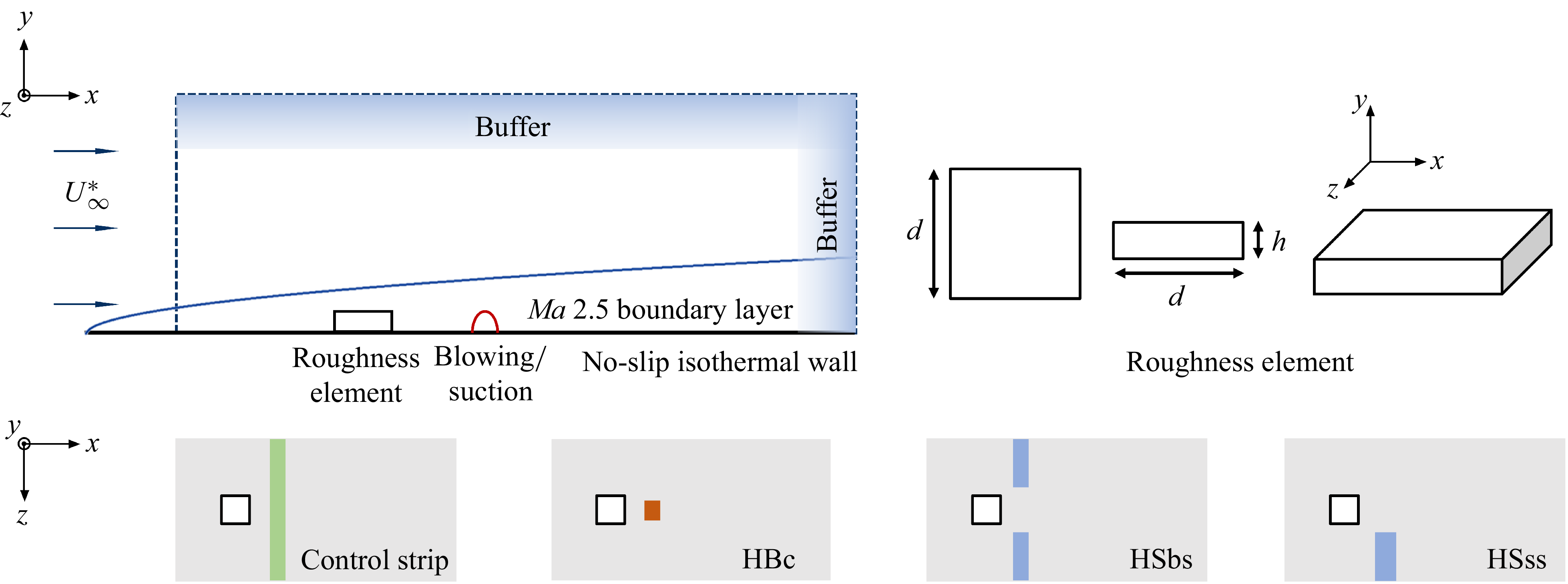
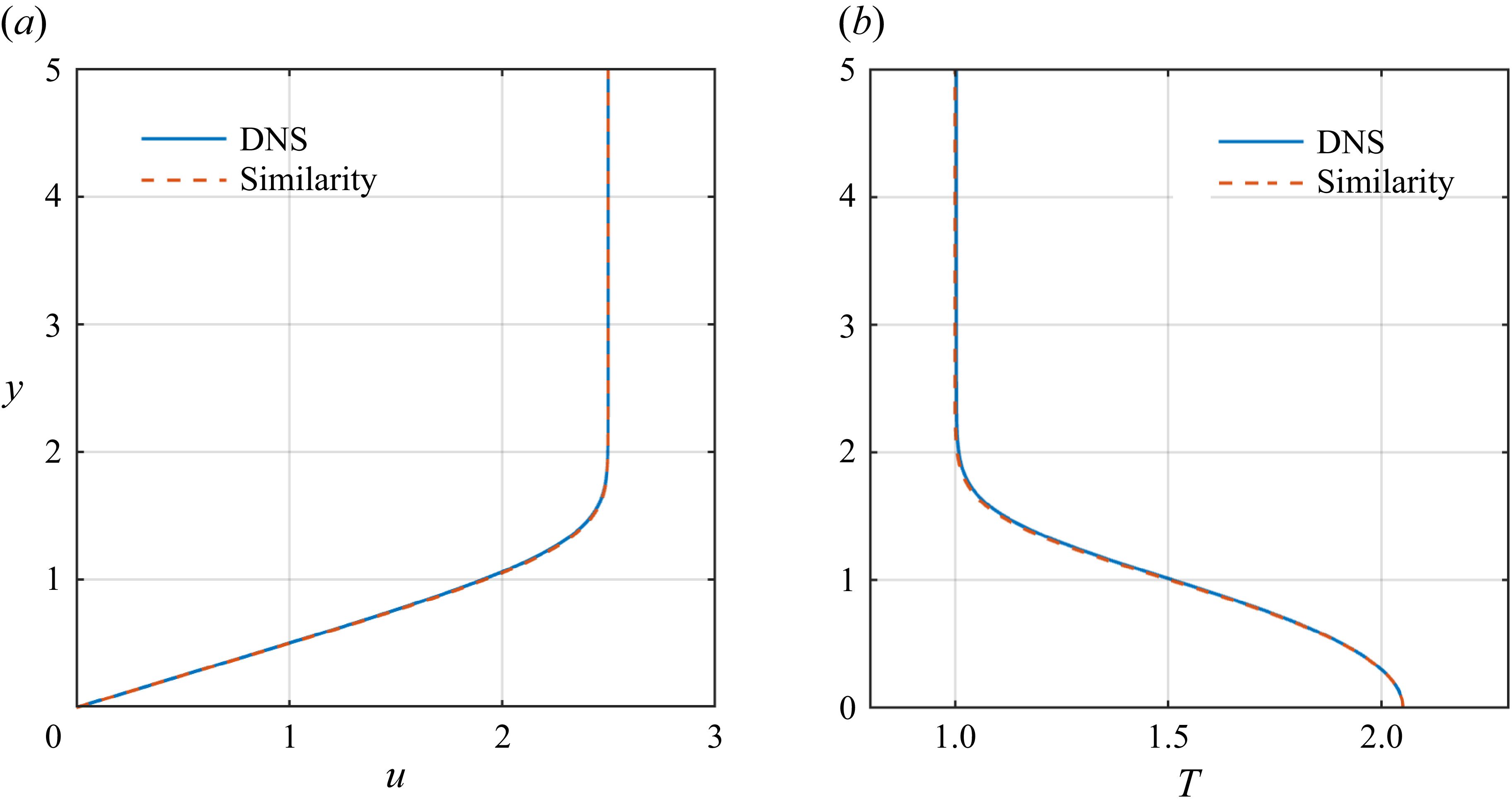
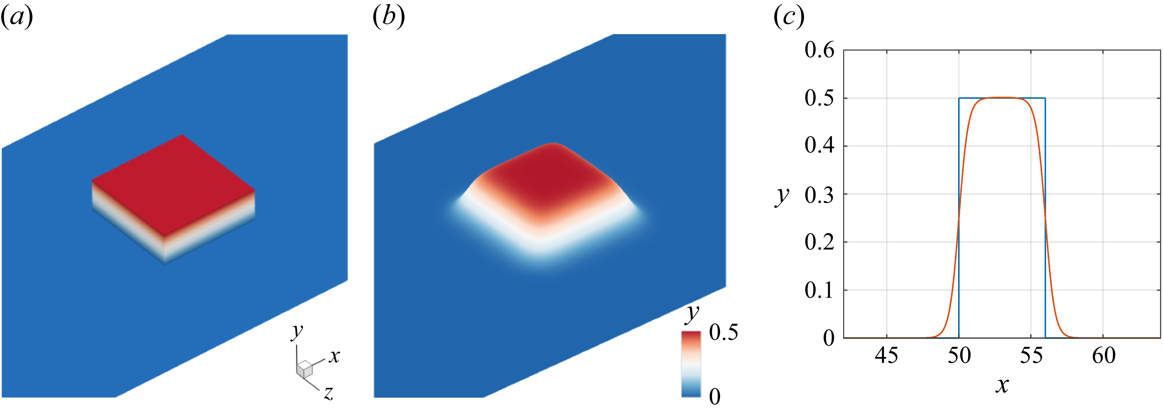
 z=0
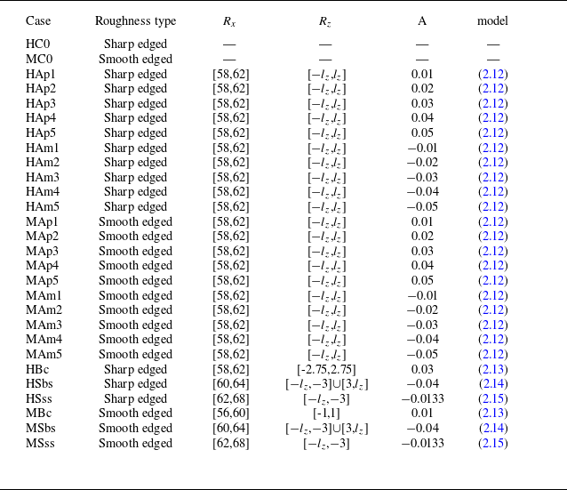
 Rx
 x
 Rz
 [−lz,lz]
 v(x,z,t)>A/2
 A
 lz=Lz/2=10
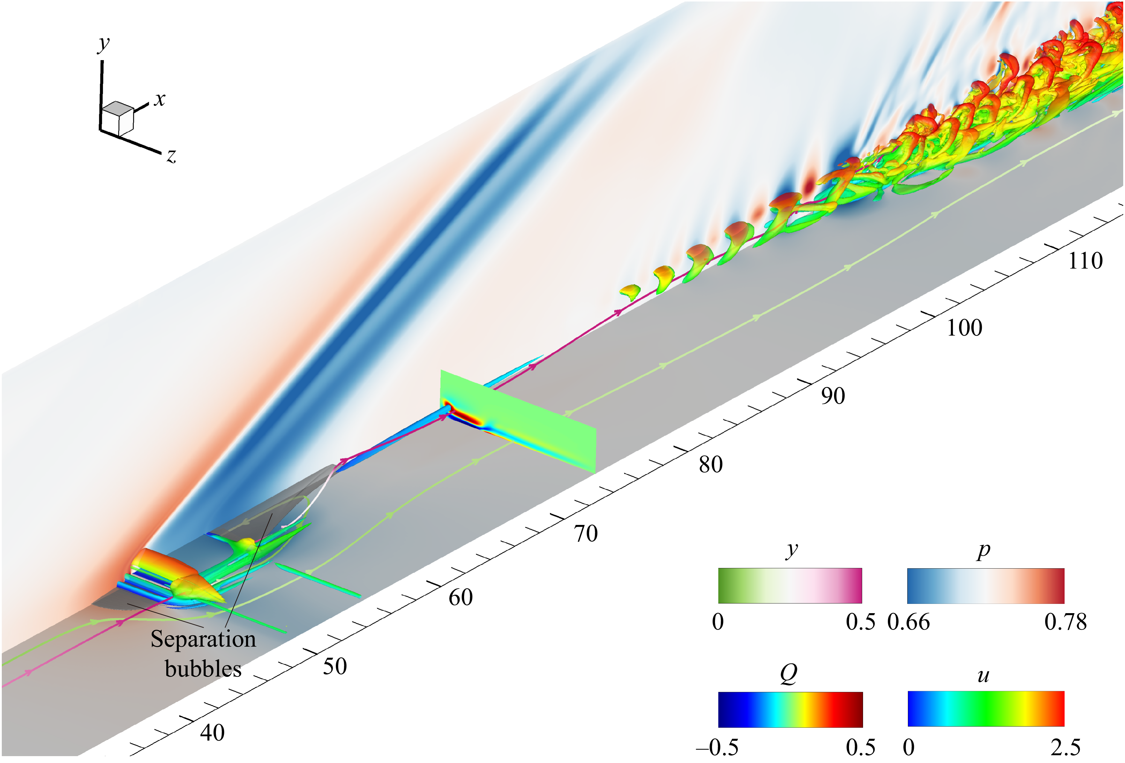
 Q=0.02
 u
 z=0
 ωx
 x=75
 u
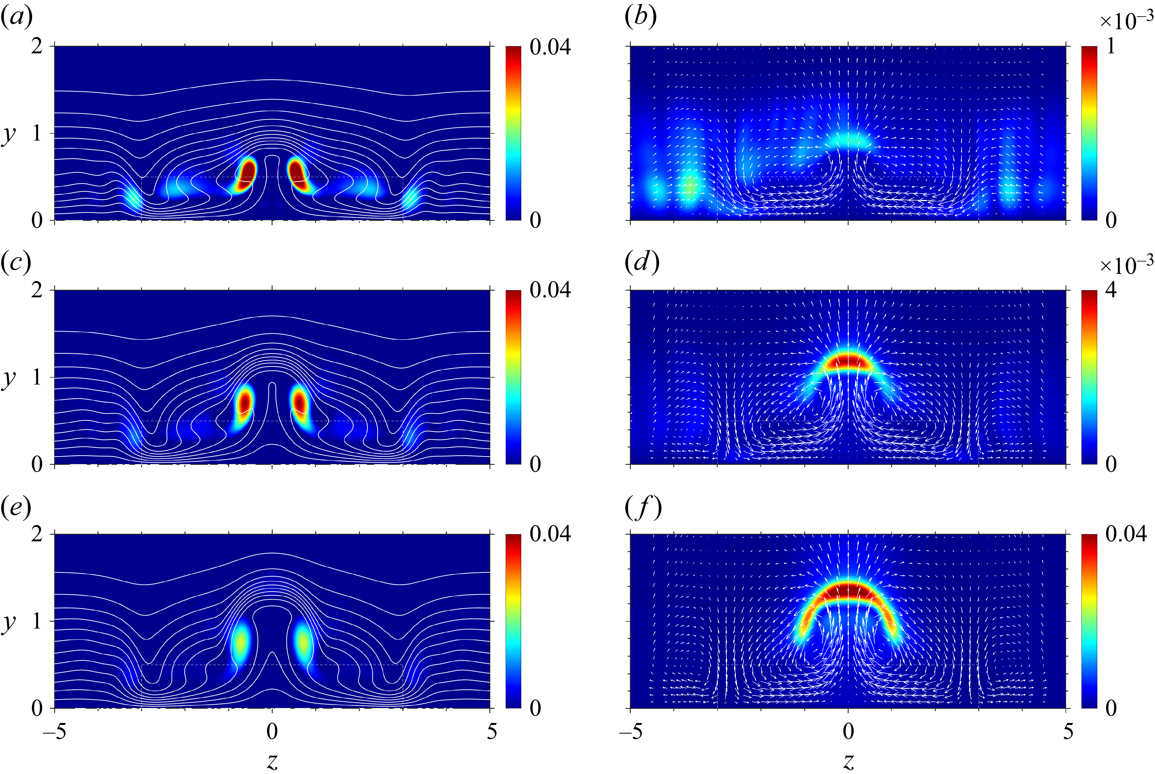
 urms′
 x=70
 x=80
 x=90
 (v,w)
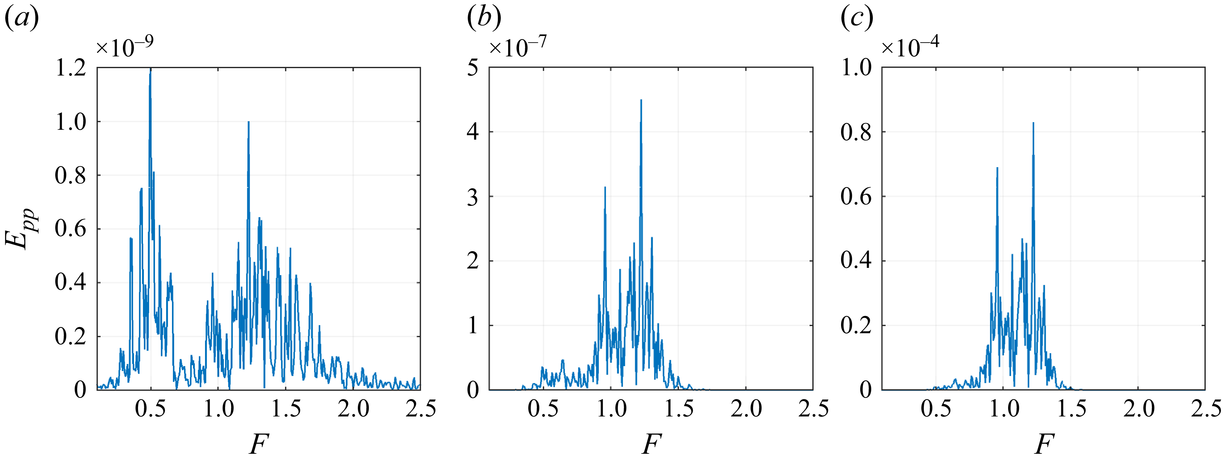
 Epp=p^wp^w+
 x=70,
 x=80
 x=90
 y=0.9,z=0
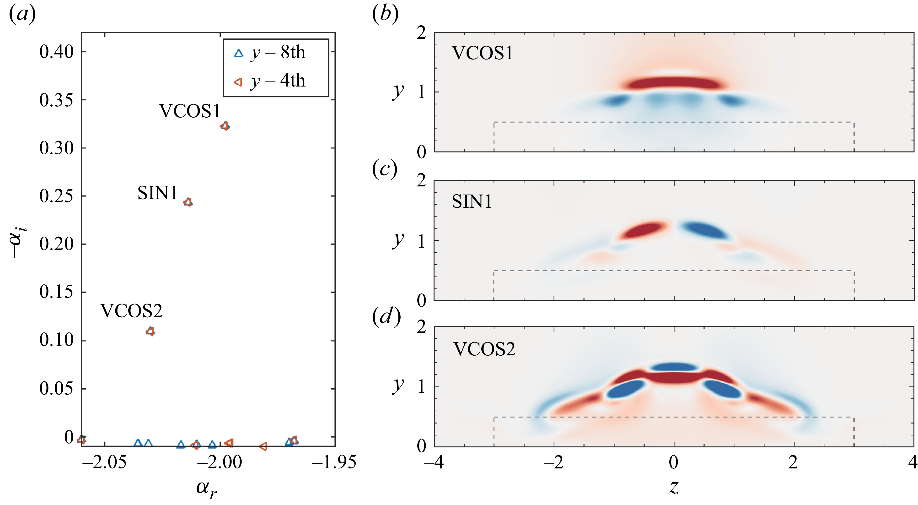
 x=80
 F=1.1
 u
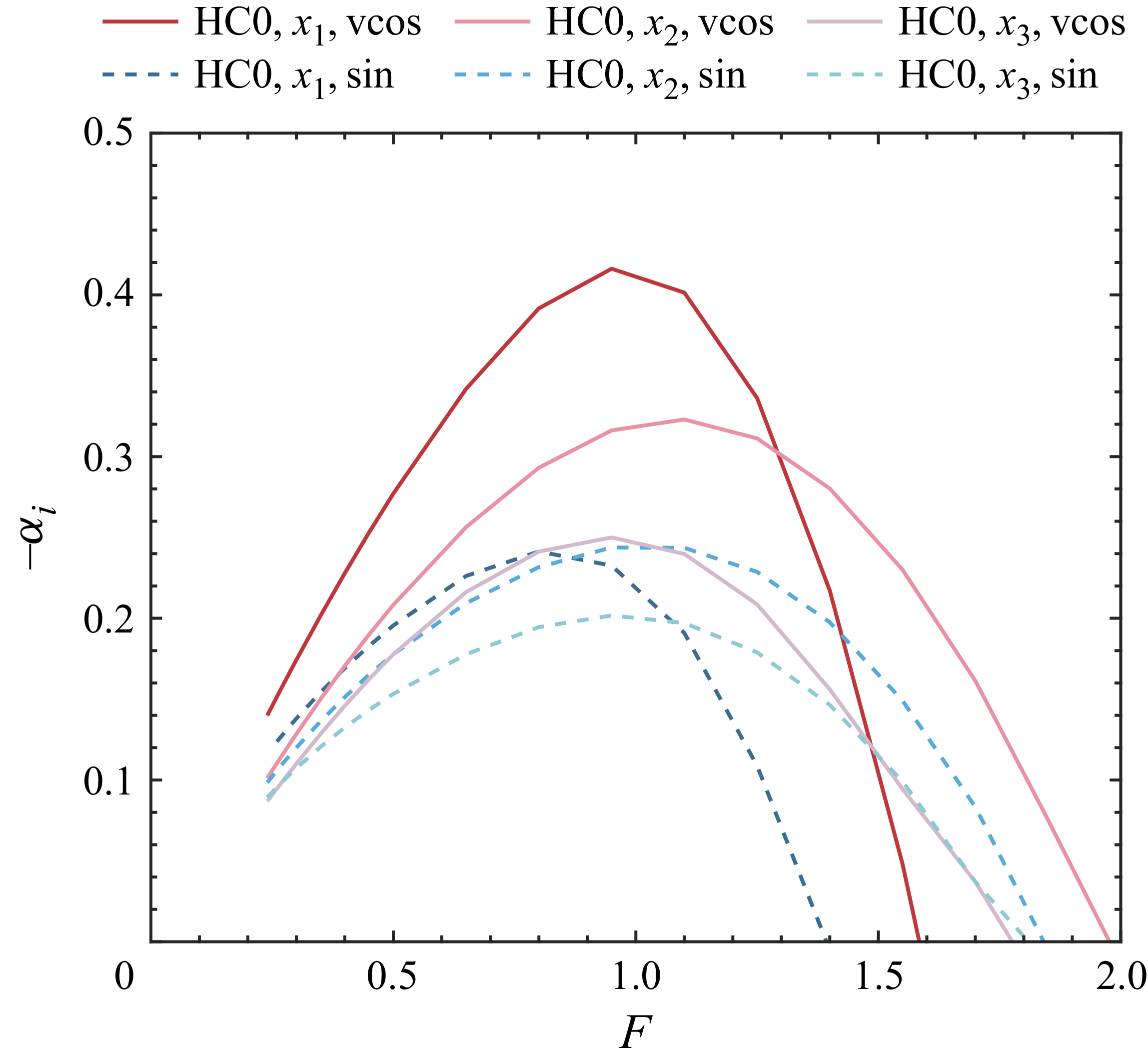
 x=70,80
 90
 x1,x2
 x3
 x=70,80
 90
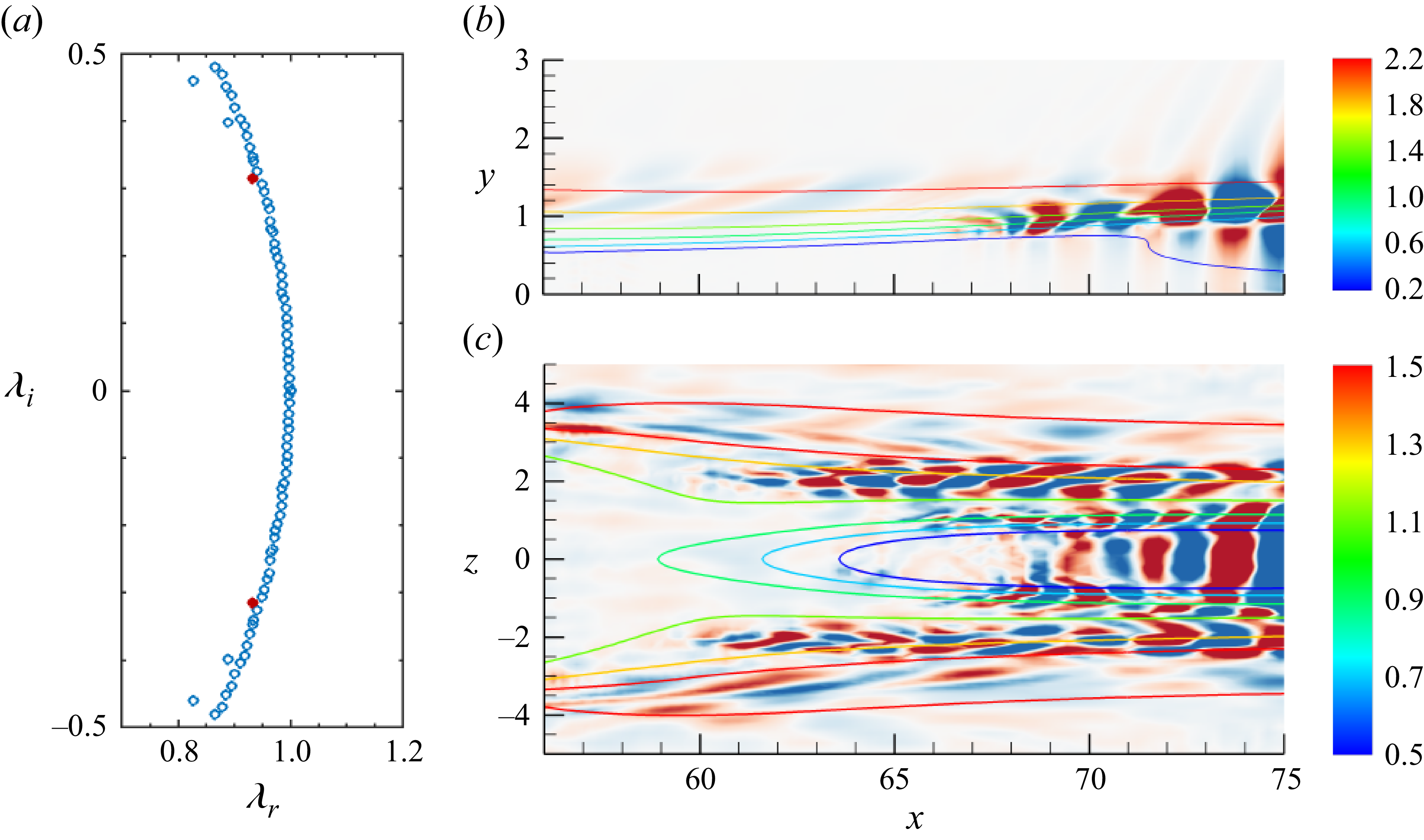
 F≈1.1
 u
 z=0
 y=0.7
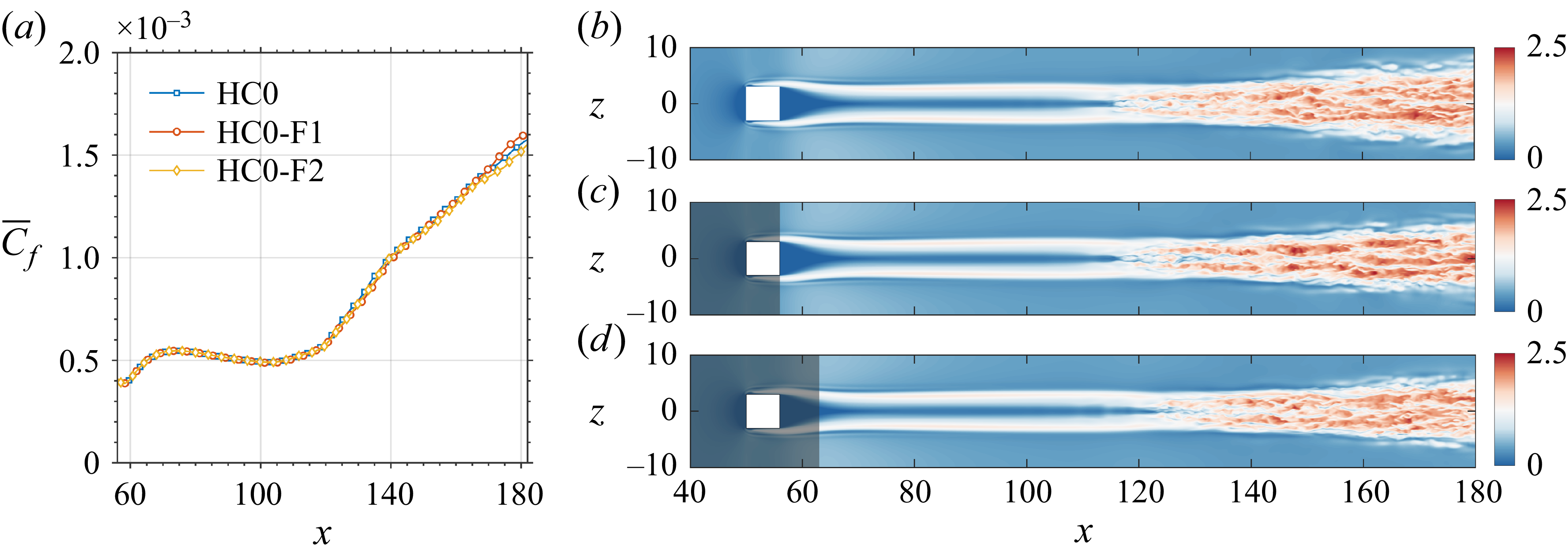
 C¯f
 u
 y=0.2

 x=70,y=0.5,z=0
 x=90,y=0.5,z=0

 C¯f
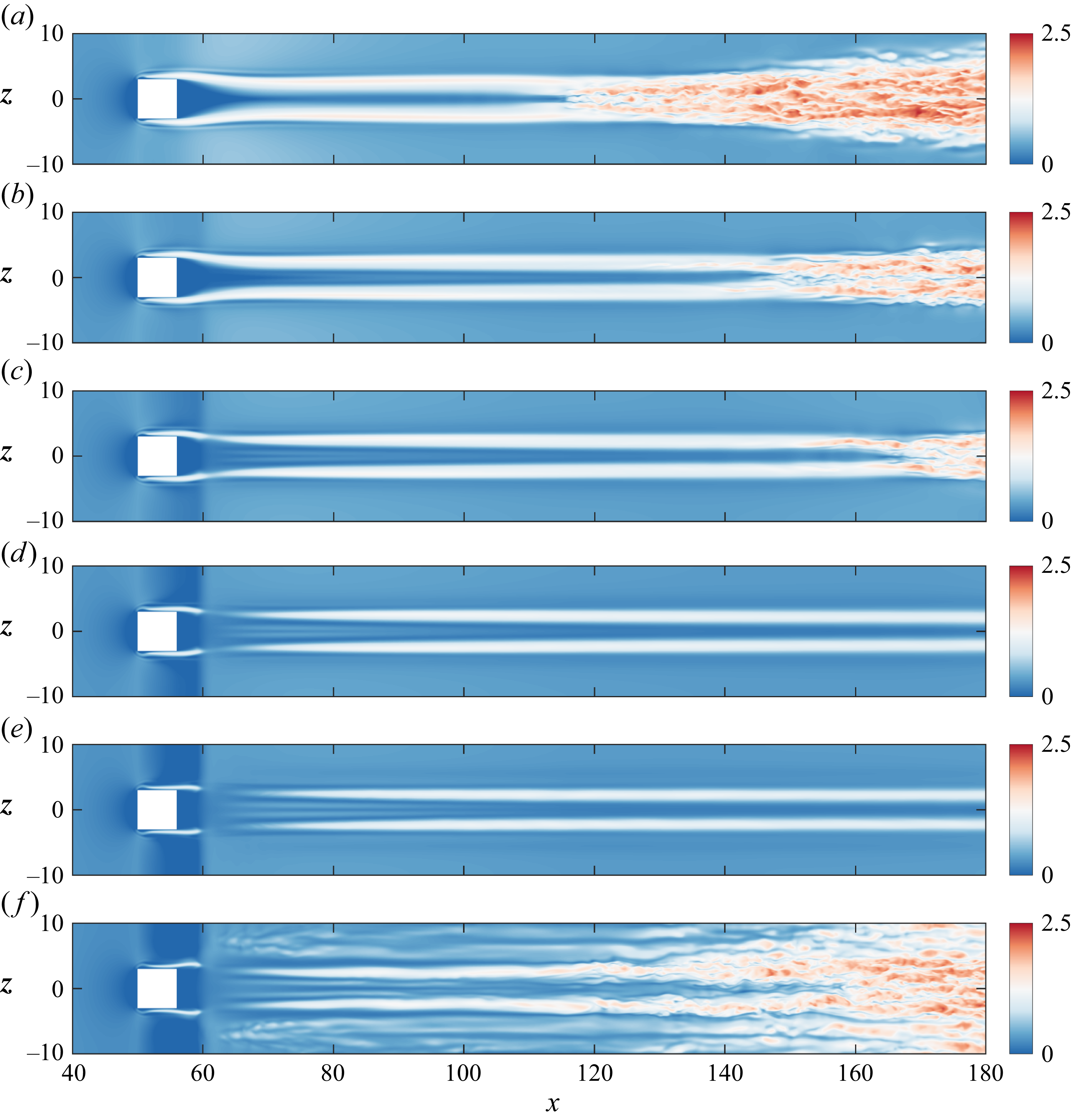
 u
 y=0.2

 x=70
 x=80
 x=90
 [0,2.5]

 urms′
 x=70
 x=80
 x=90
 (v,w)
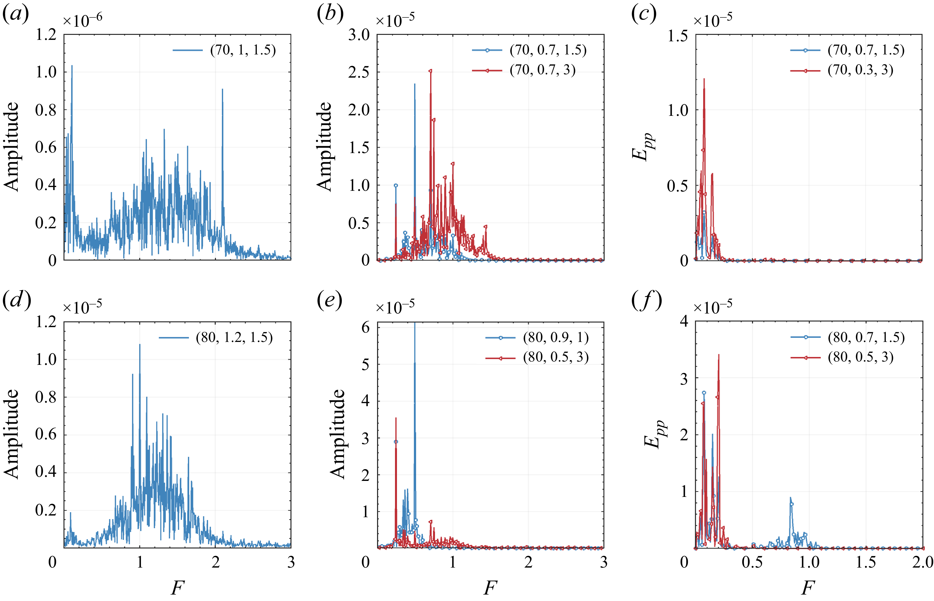
 (x,y,z)
 x=70
 x=80

 x1,x2
 x3
 x=70,80
 90
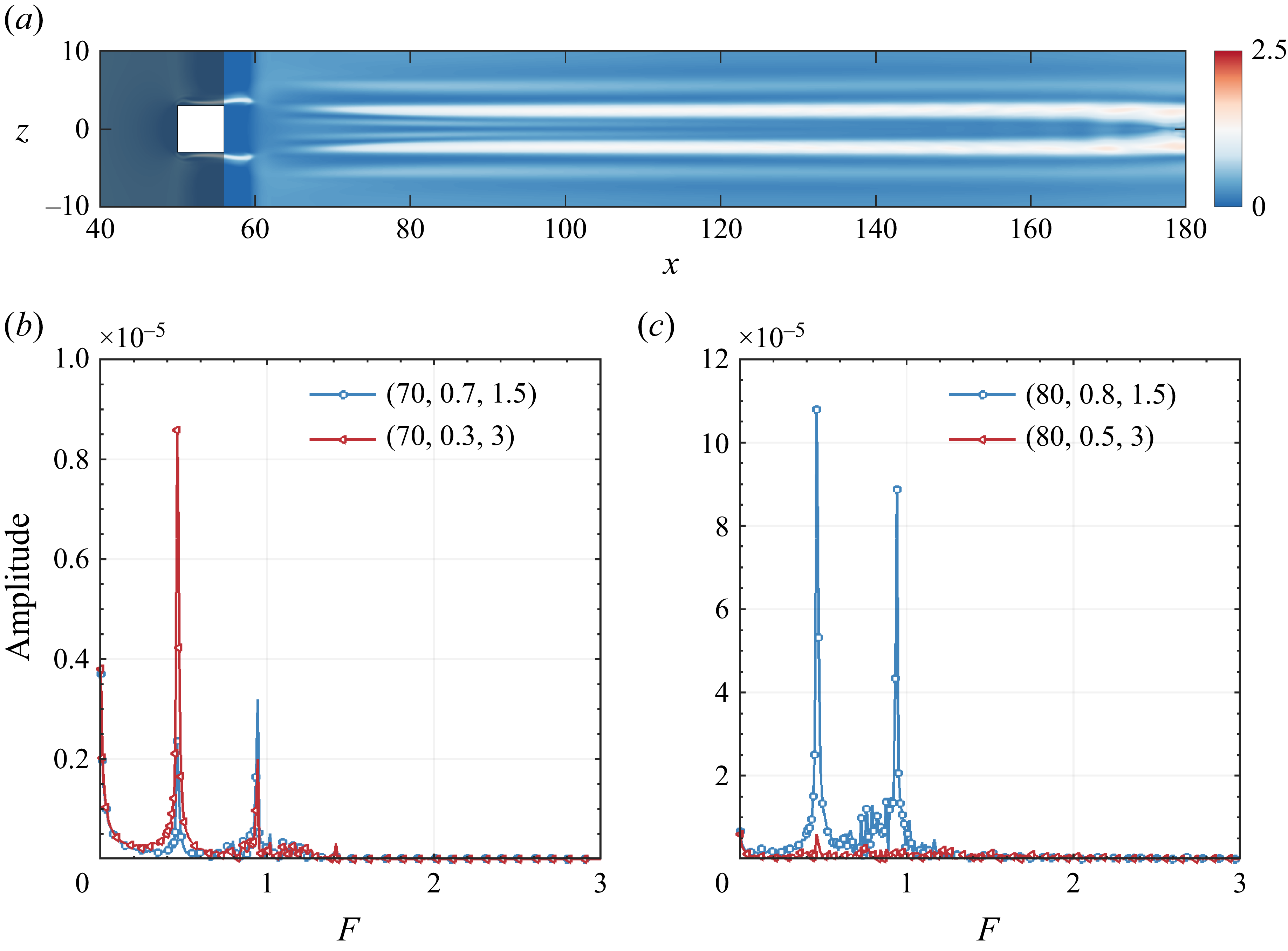
 x<56
 y=0.2
 x=70
 x=80
 (x,y,z)
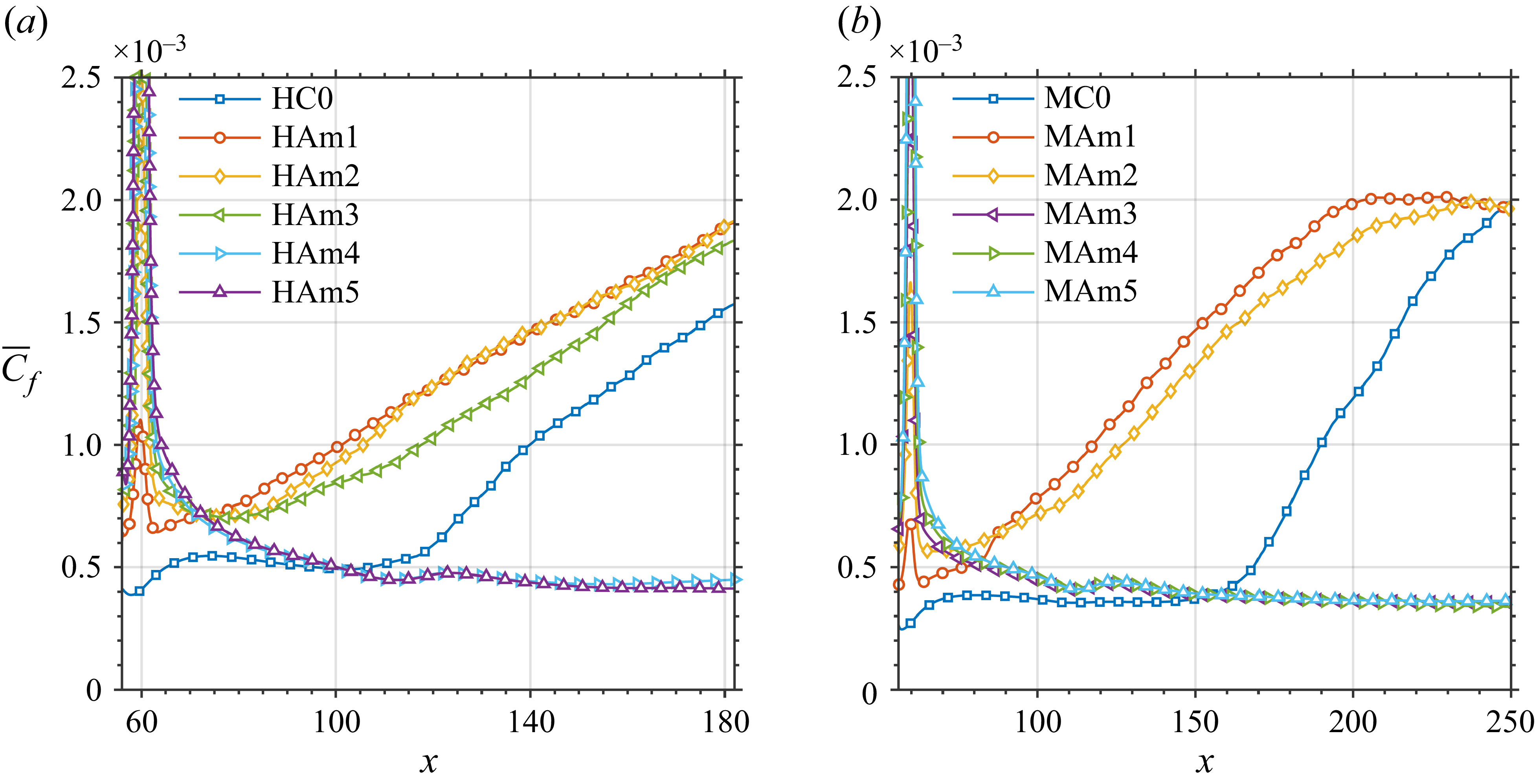
 C¯f
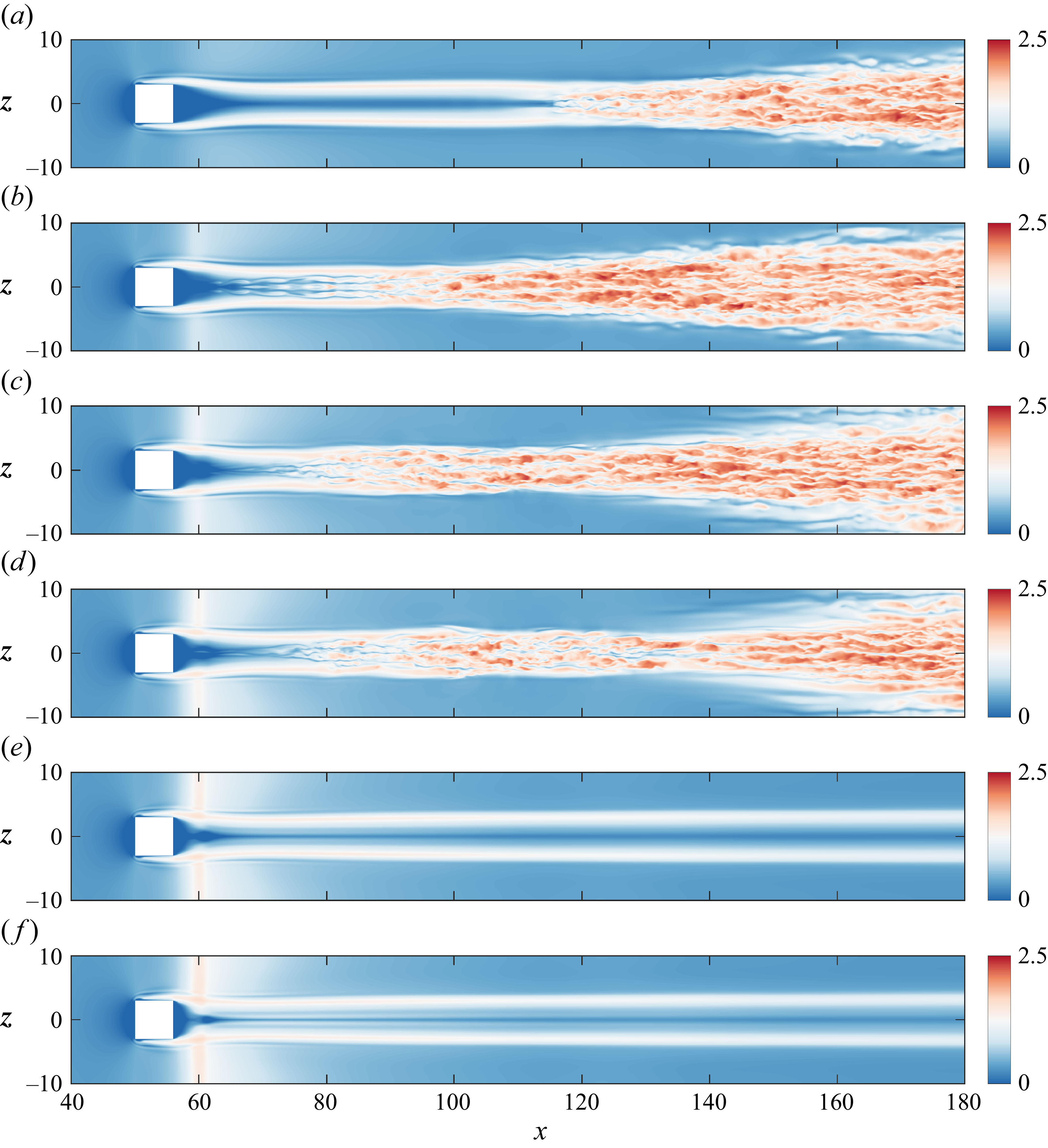
 u
 y=0.2

 x=70
 x=80
 x=90
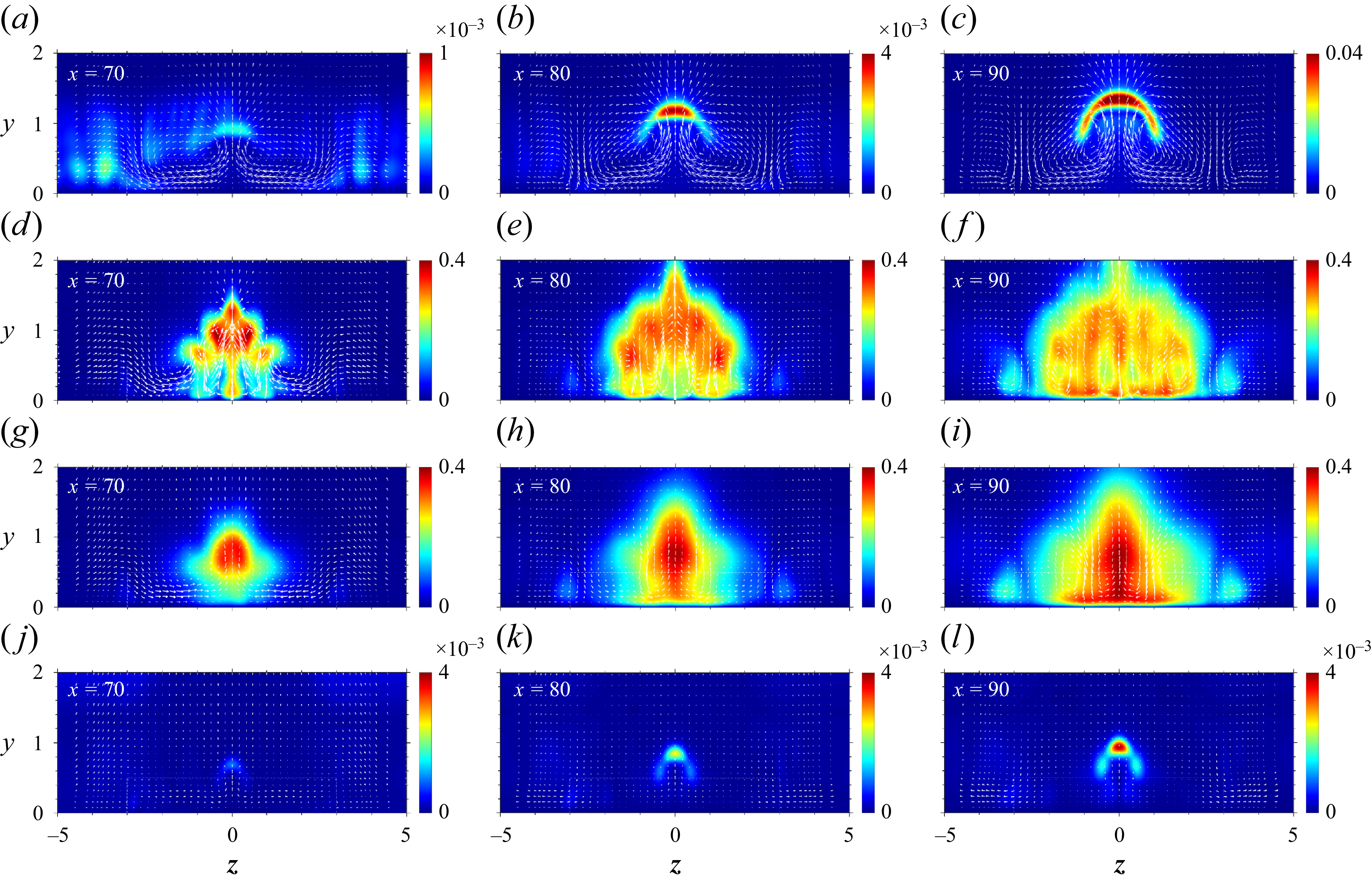
 urms′
 x=70
 x=80
 x=90
 (v,w)
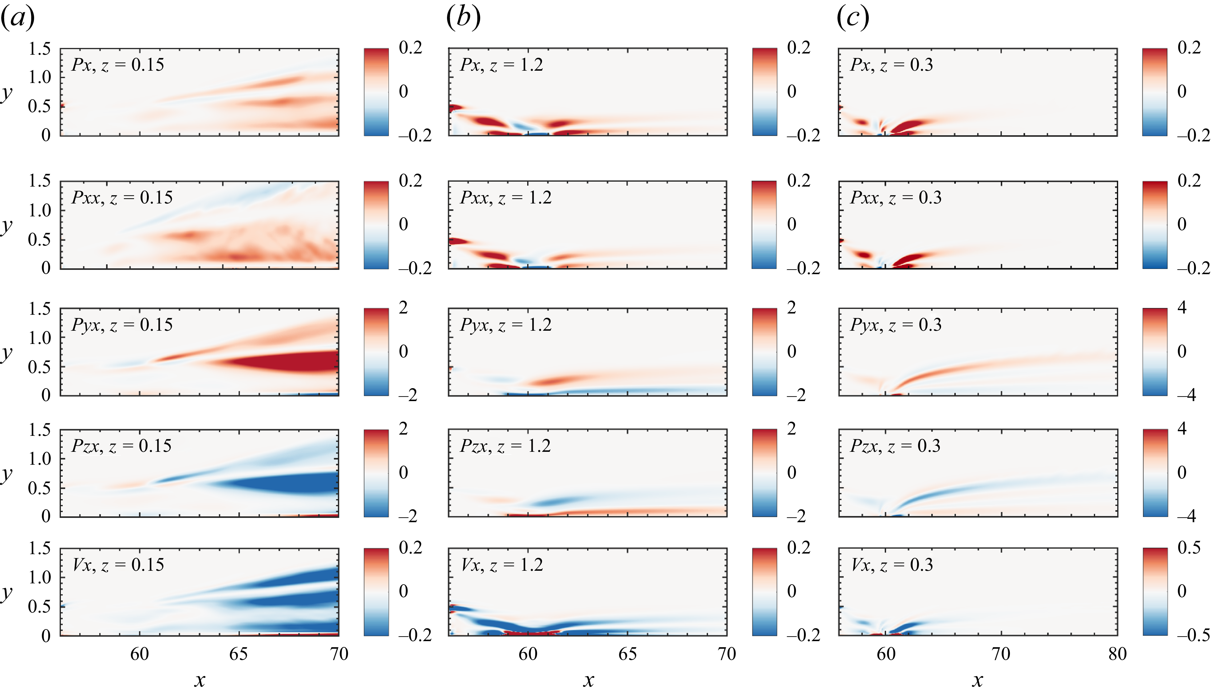
 Px
 Pxx
 Pyx
 Pzx
 Vx
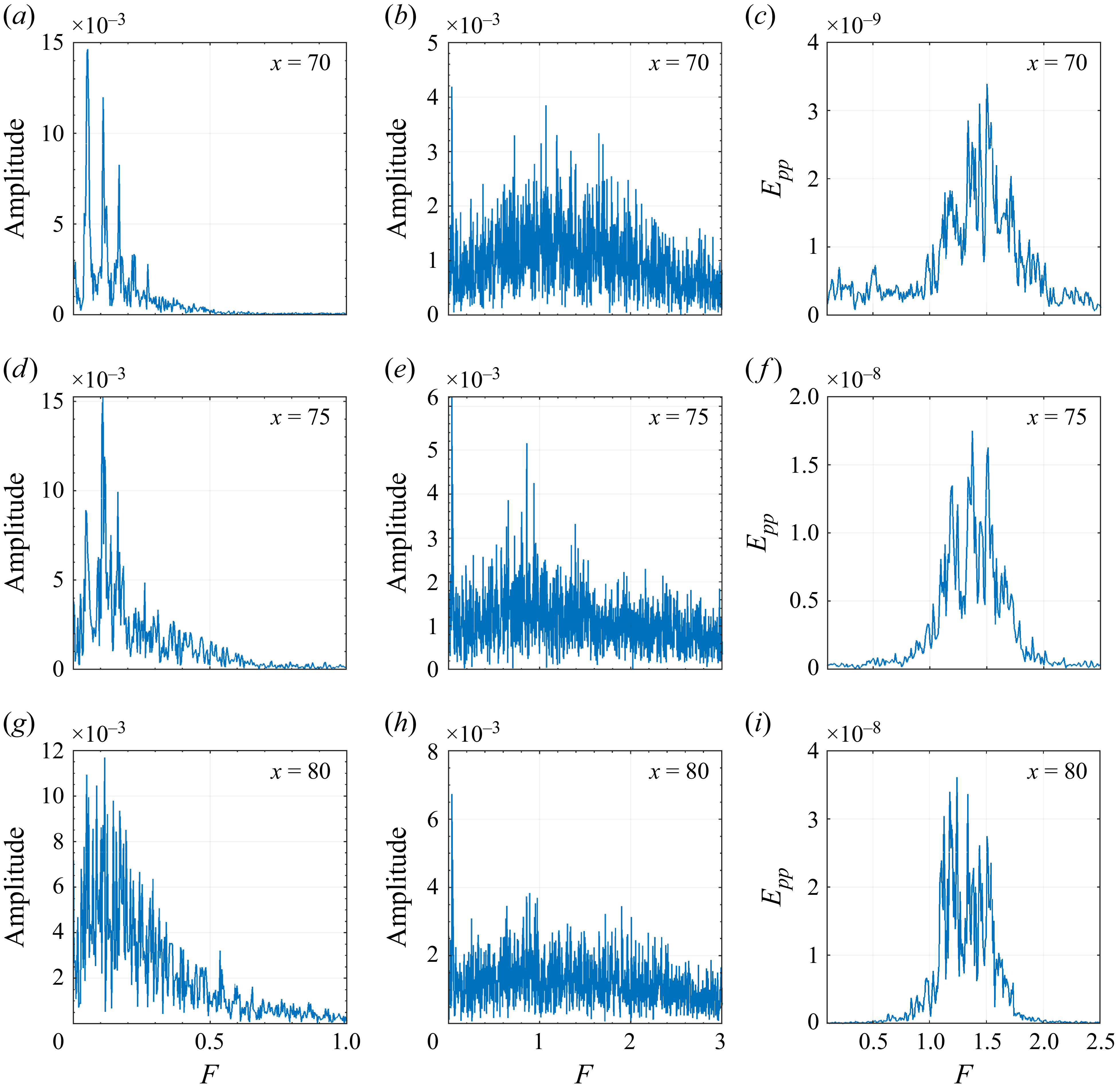
 Epp
 x=70
 x=75
 x=80
 y=0.9
 z=0
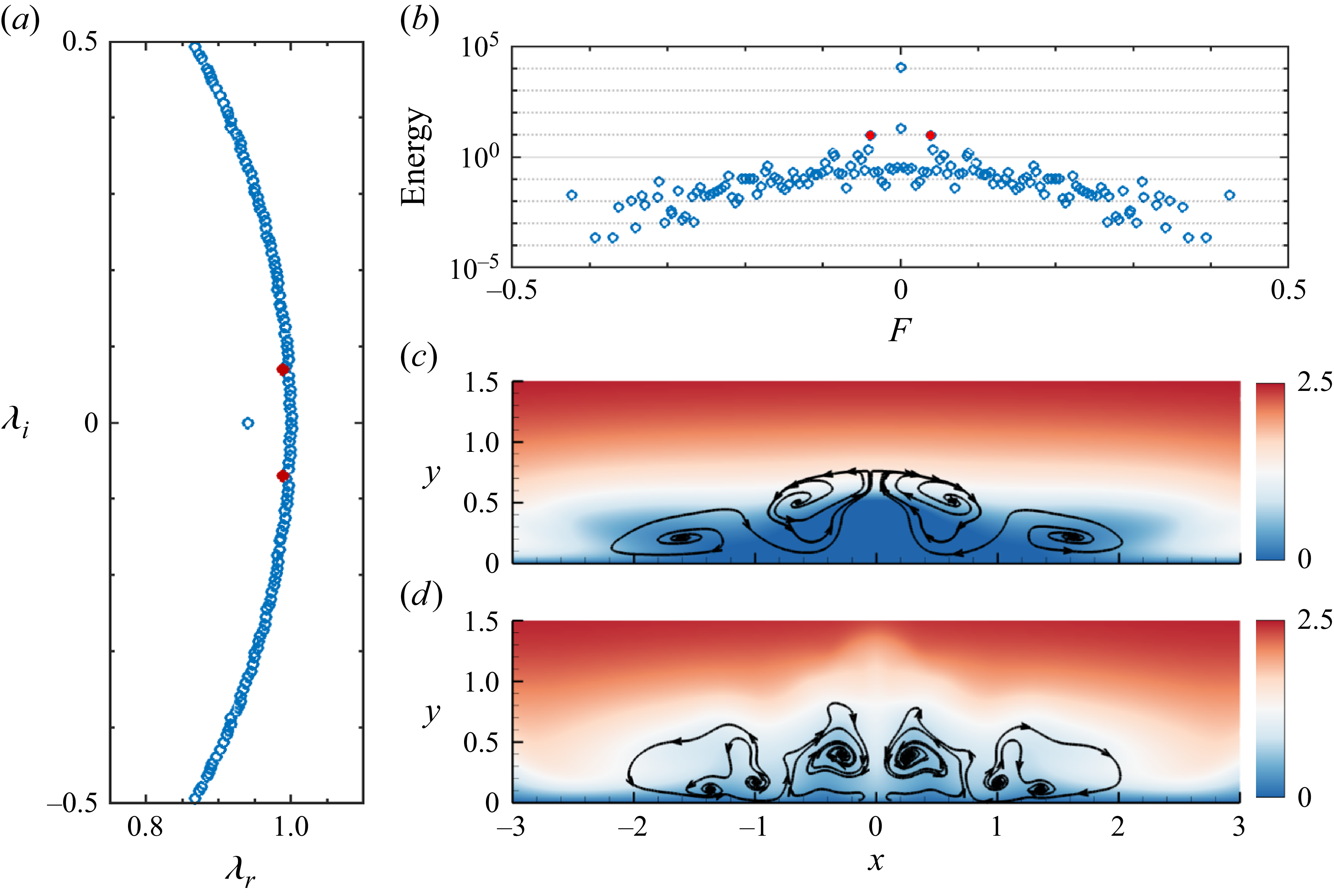
 F≈0.04
 x=60
 x=70
 v−w
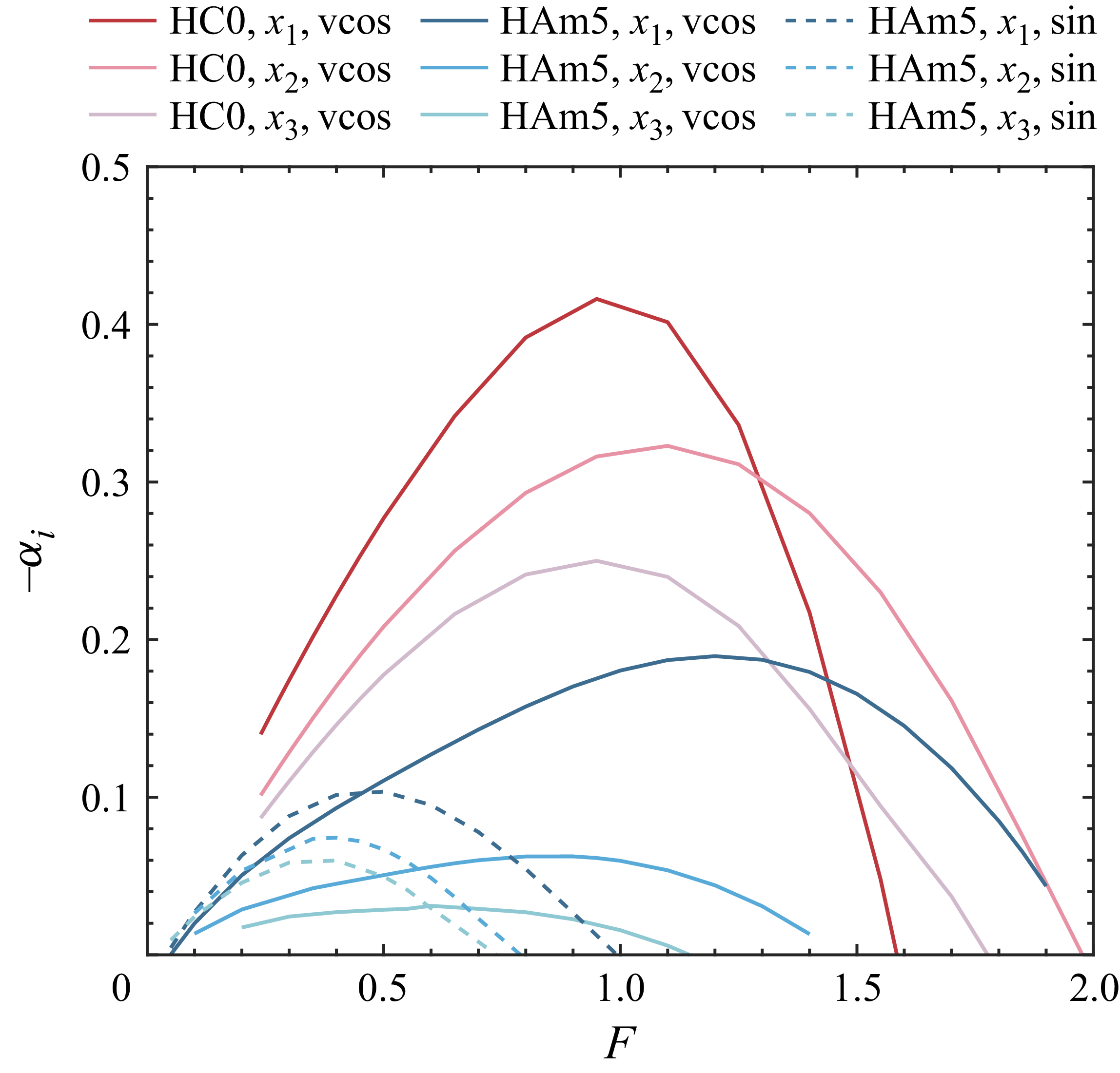
 x1,x2
 x3
 x=70,80
 90

 C¯f
 u
 y=0.2
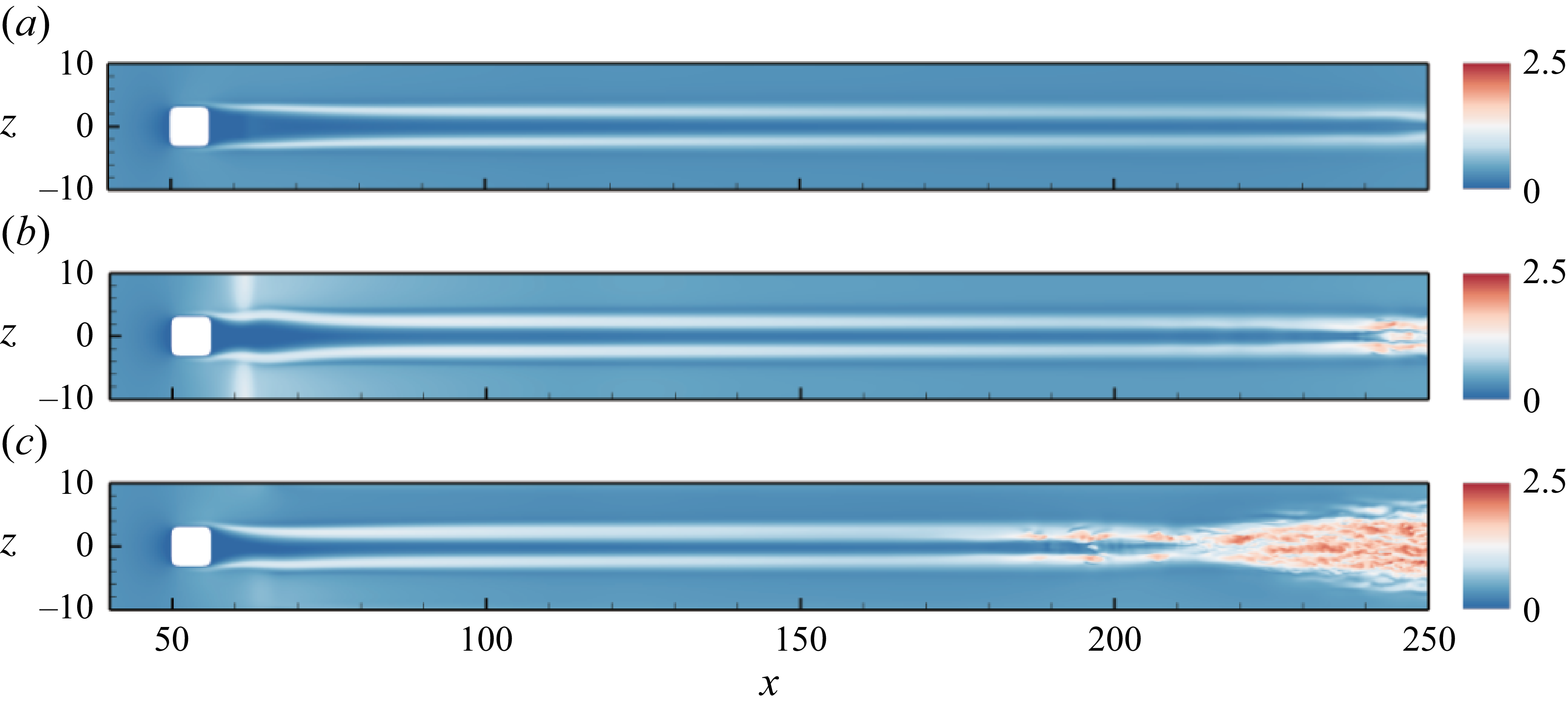
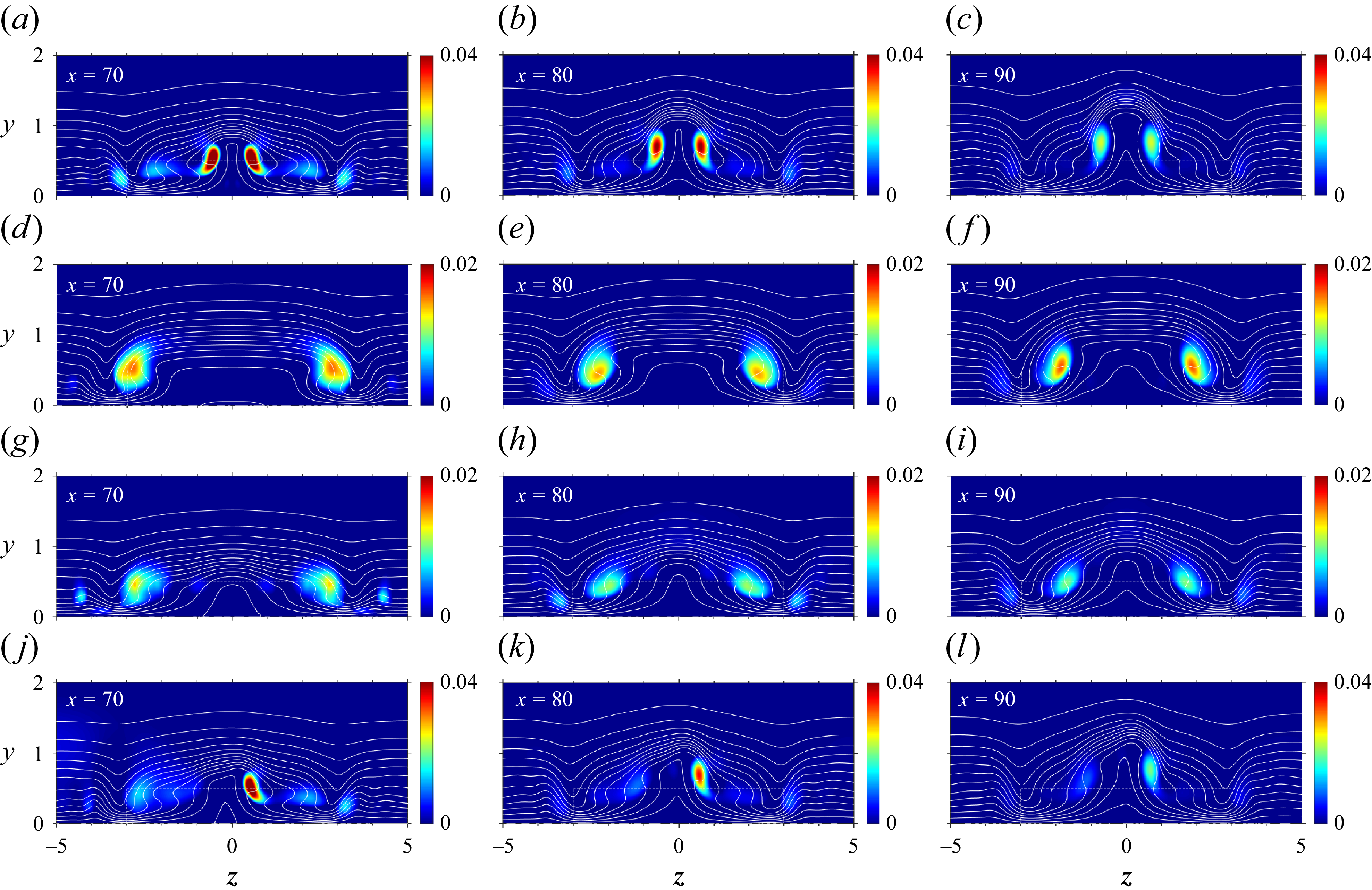
 x=70
 x=80
 x=90
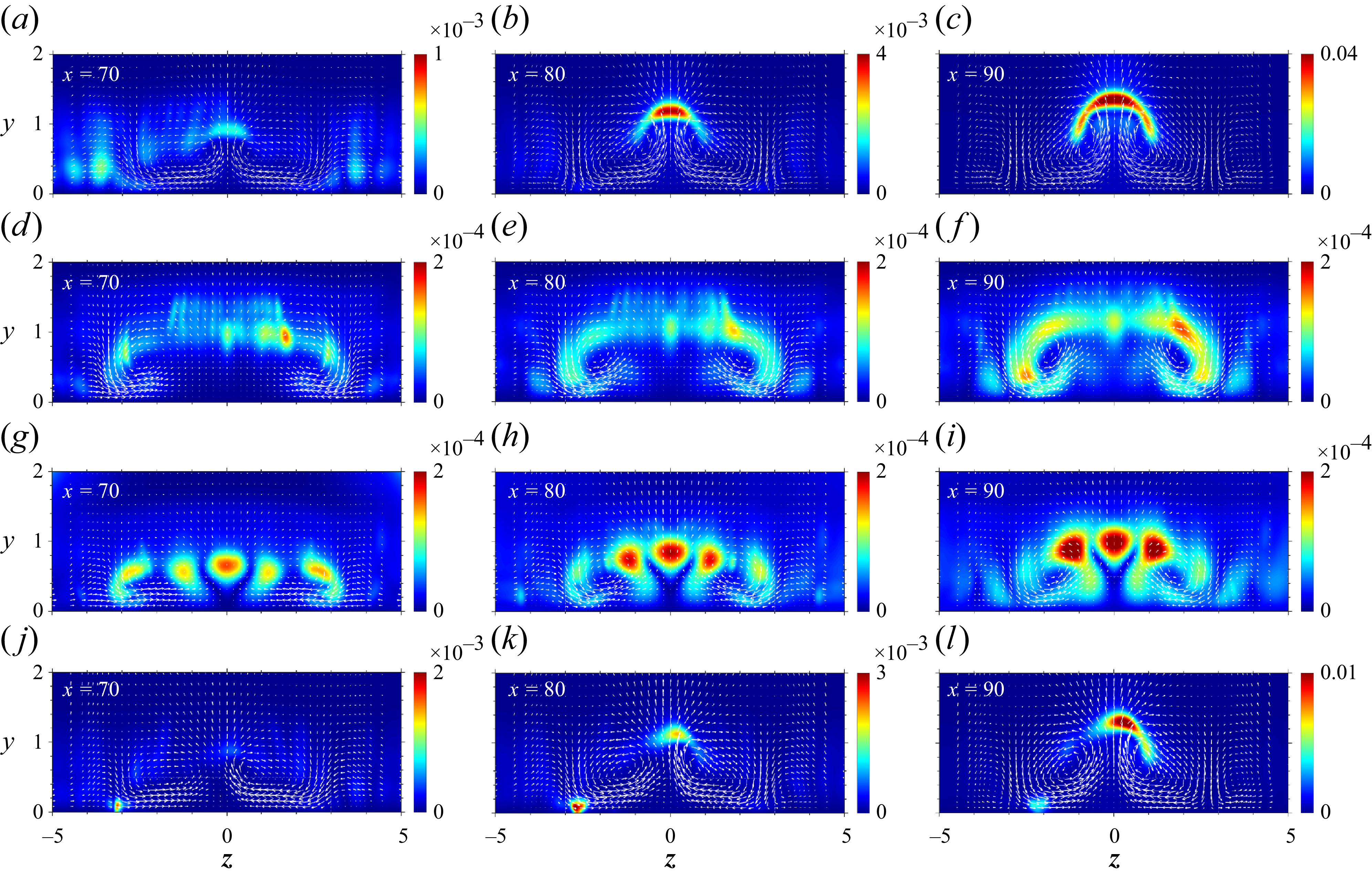
 urms′
 x=70
 x=80
 x=90
 (v,w)
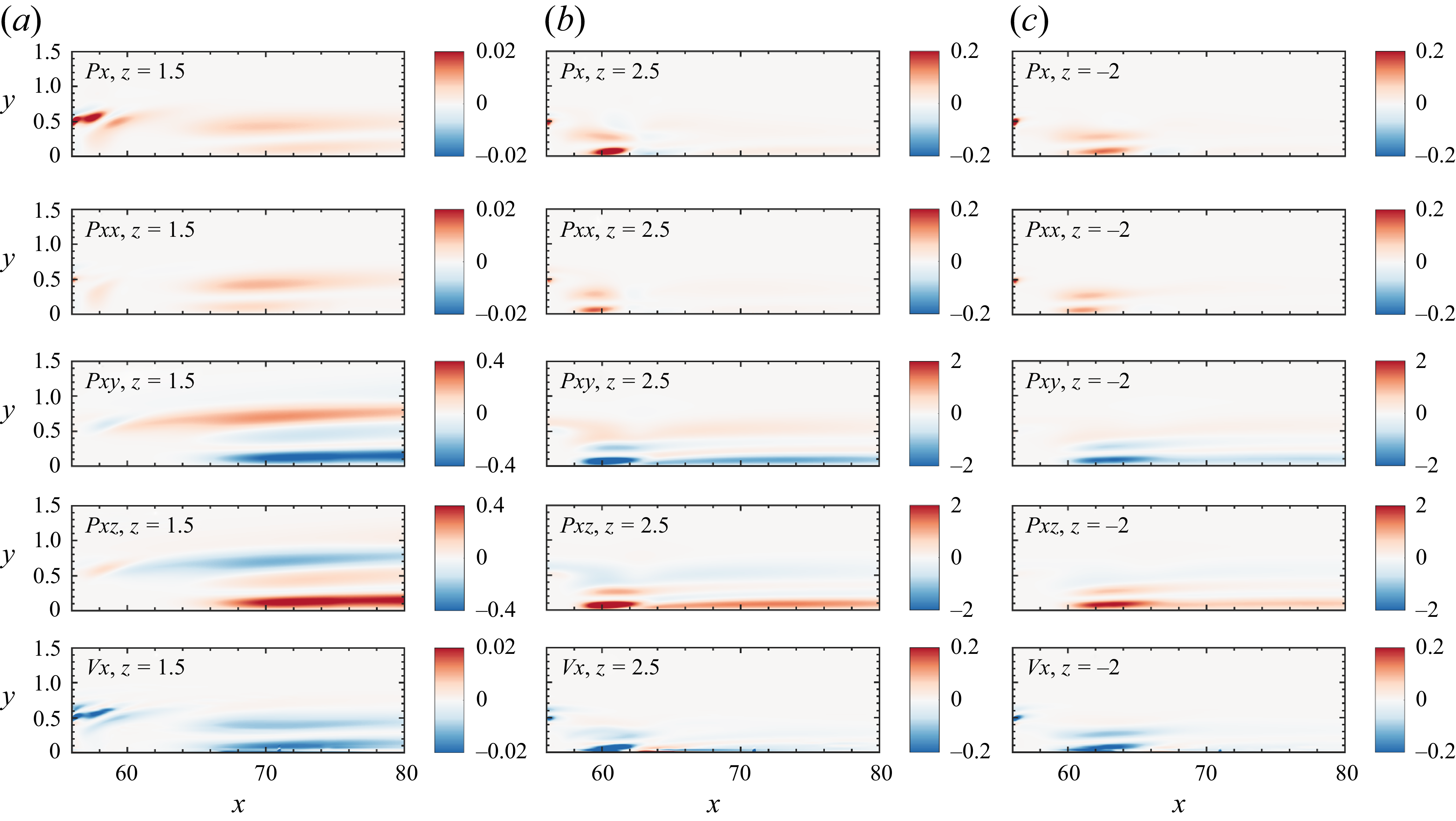
 Px
 Pxx
 Pyx
 Pzx
 Vx
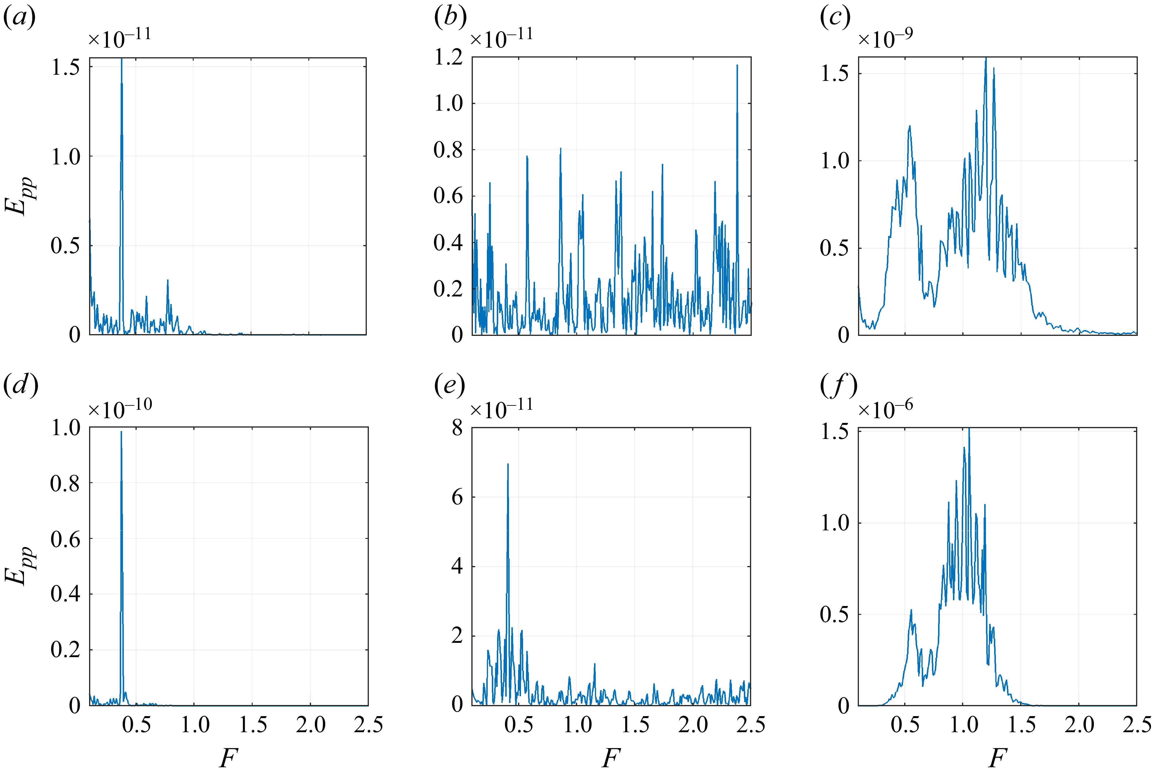
 Epp
 x=75
 x=90
 y=1.2,z=3
 y=0.9,z=0
 y=1.2,z=0.35
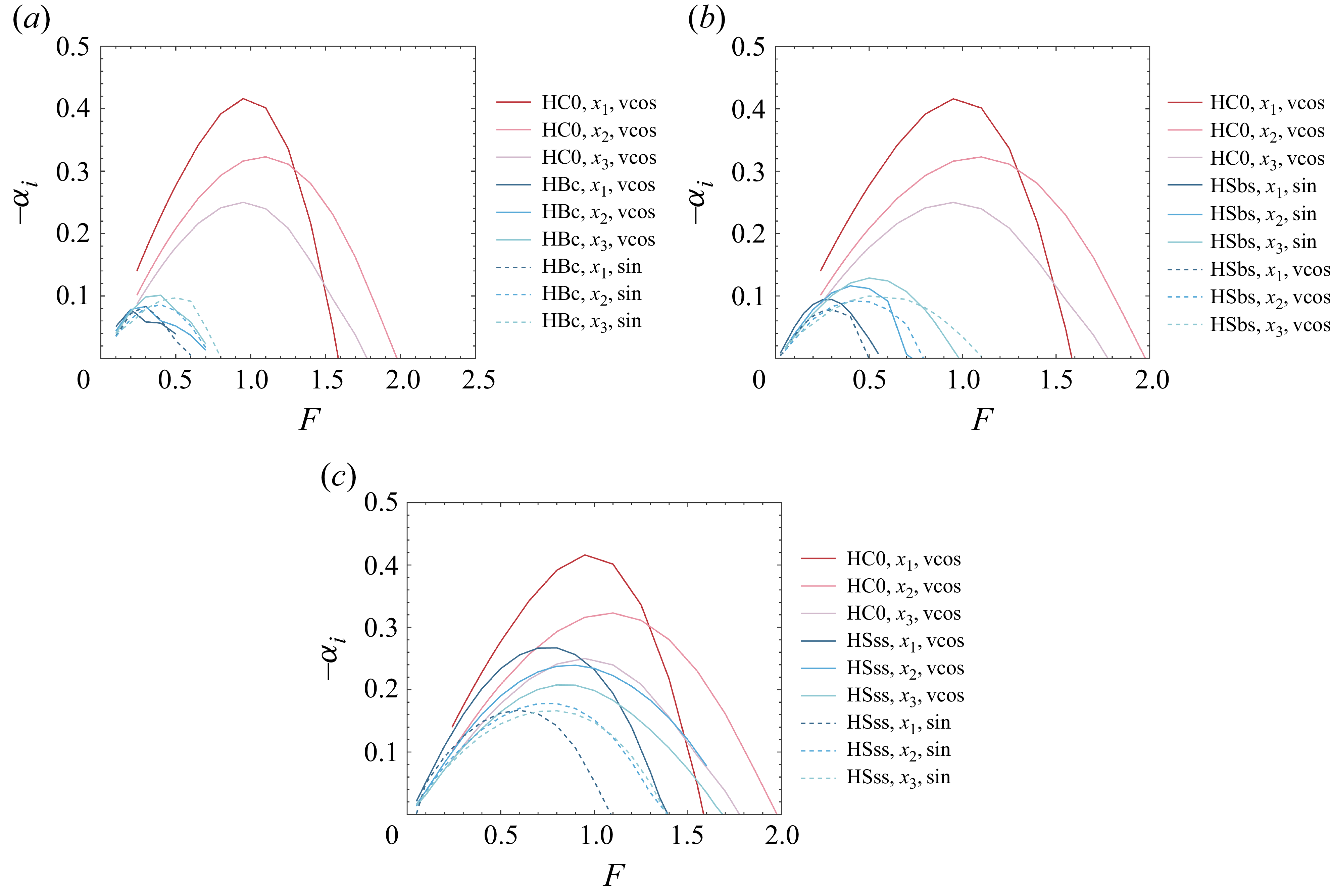
 x1,x2
 x3
 x=70,80
 90

 F=1.1
 x=80
 u
 v,w
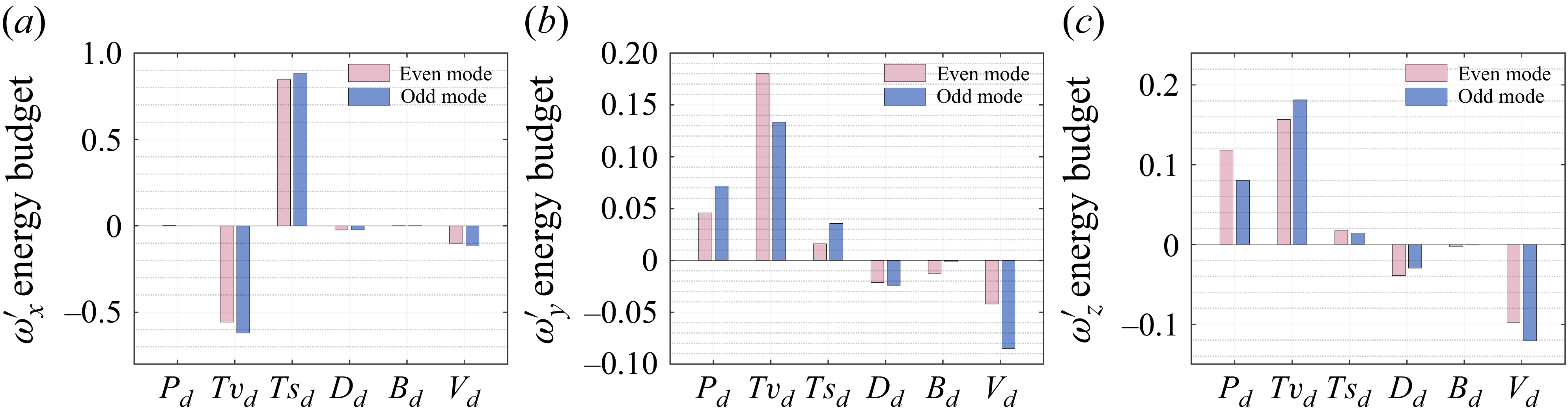
 ωx′
 ωy′
 ωz′
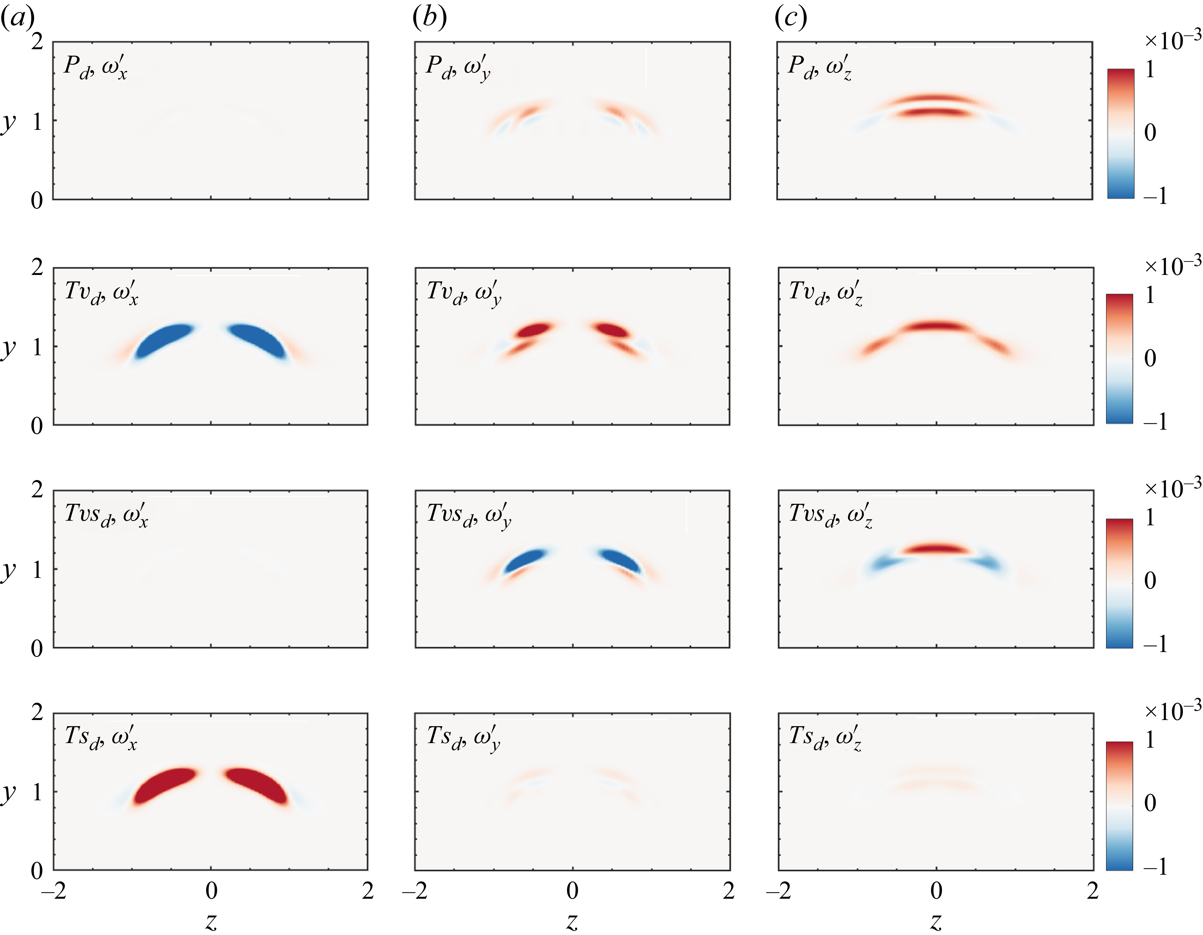
 Pd
 Tvd
 TvSd
 Tsd
 ωx′
 ωy′
 ωz′
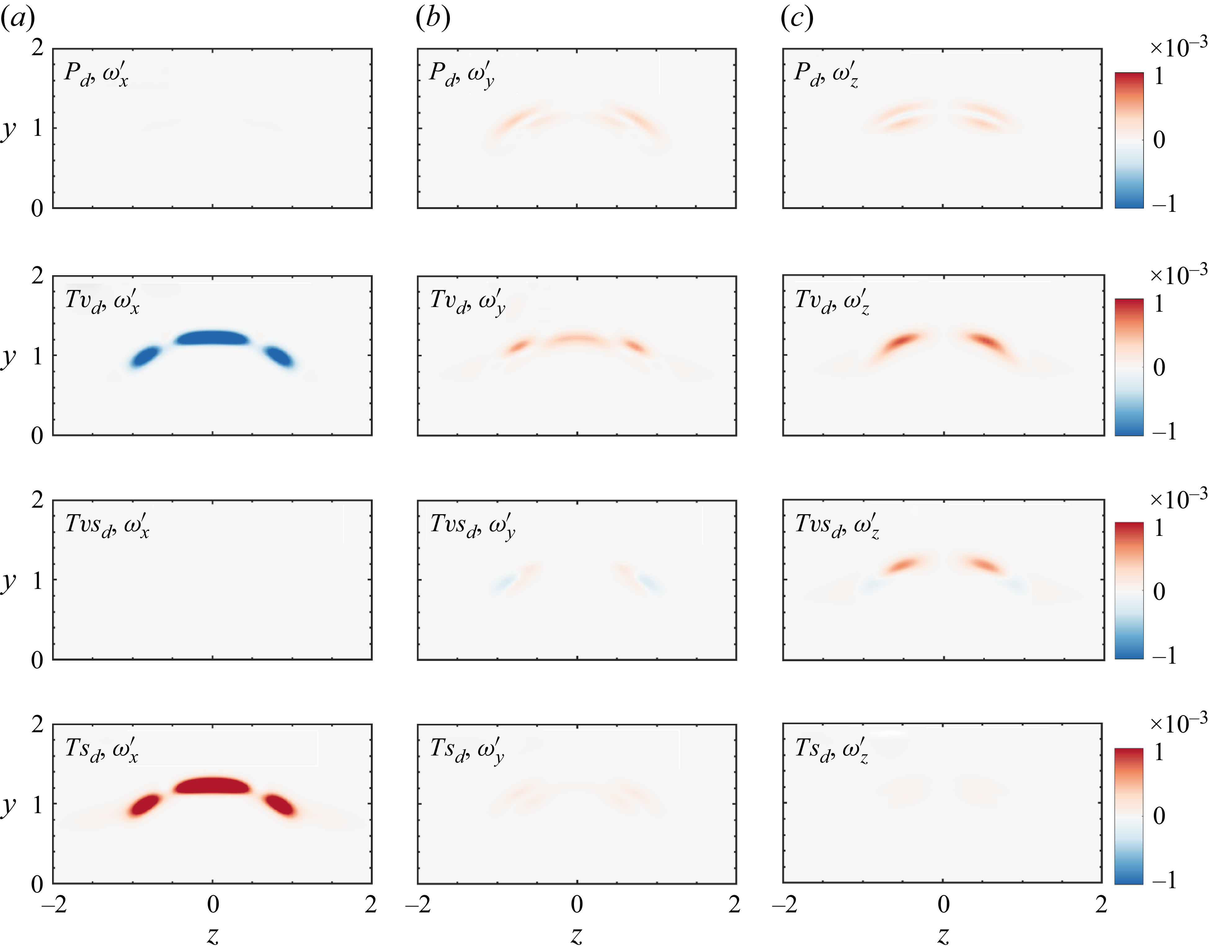
 Pd
 Tvd
 Tvsd
 Tsd
 ωx′
 ωy′
 ωz′

 ωx′
 ωy′
 ωz′
 F=
 x=80

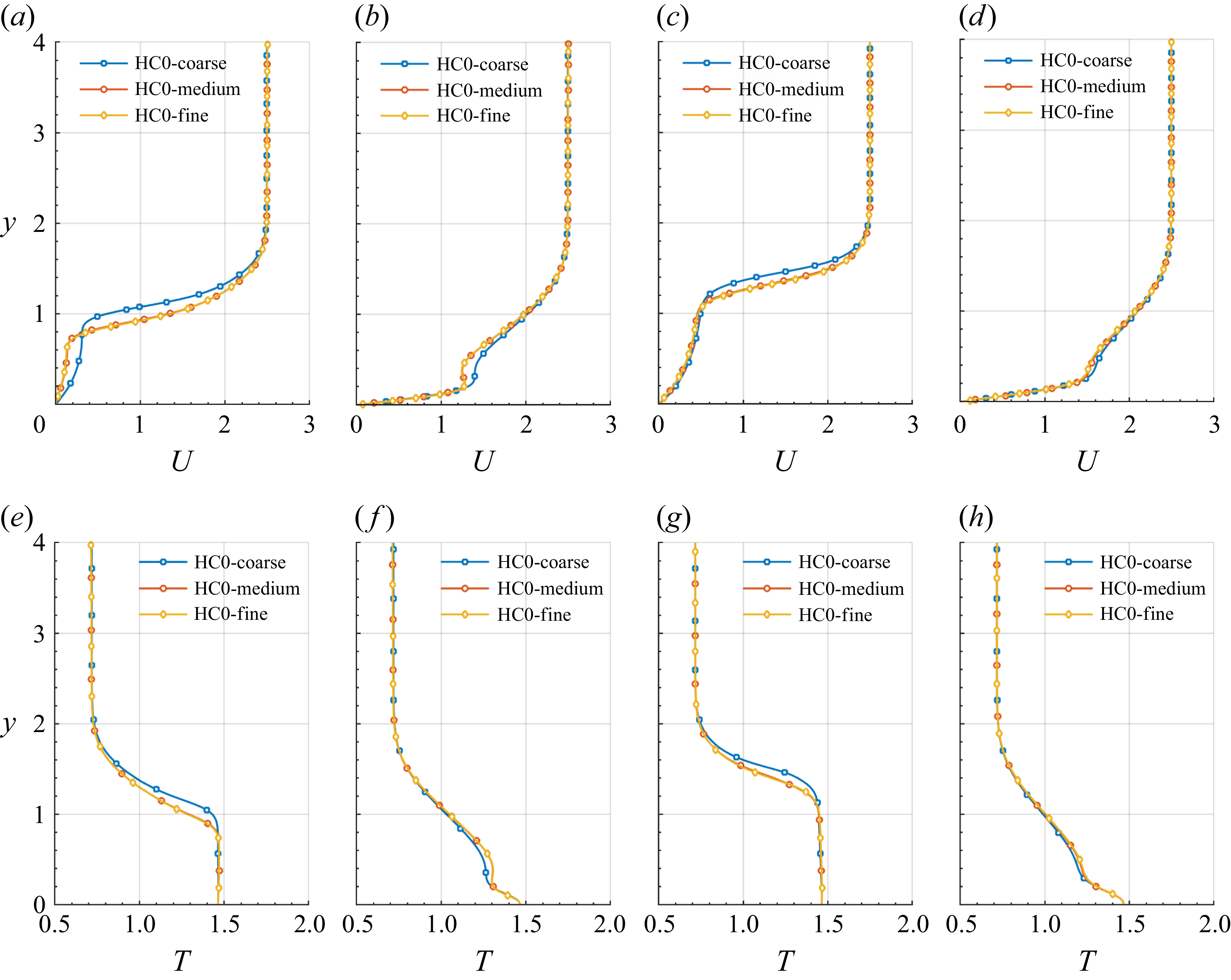
 x=70
 x=90
 z=0
 z=2.5
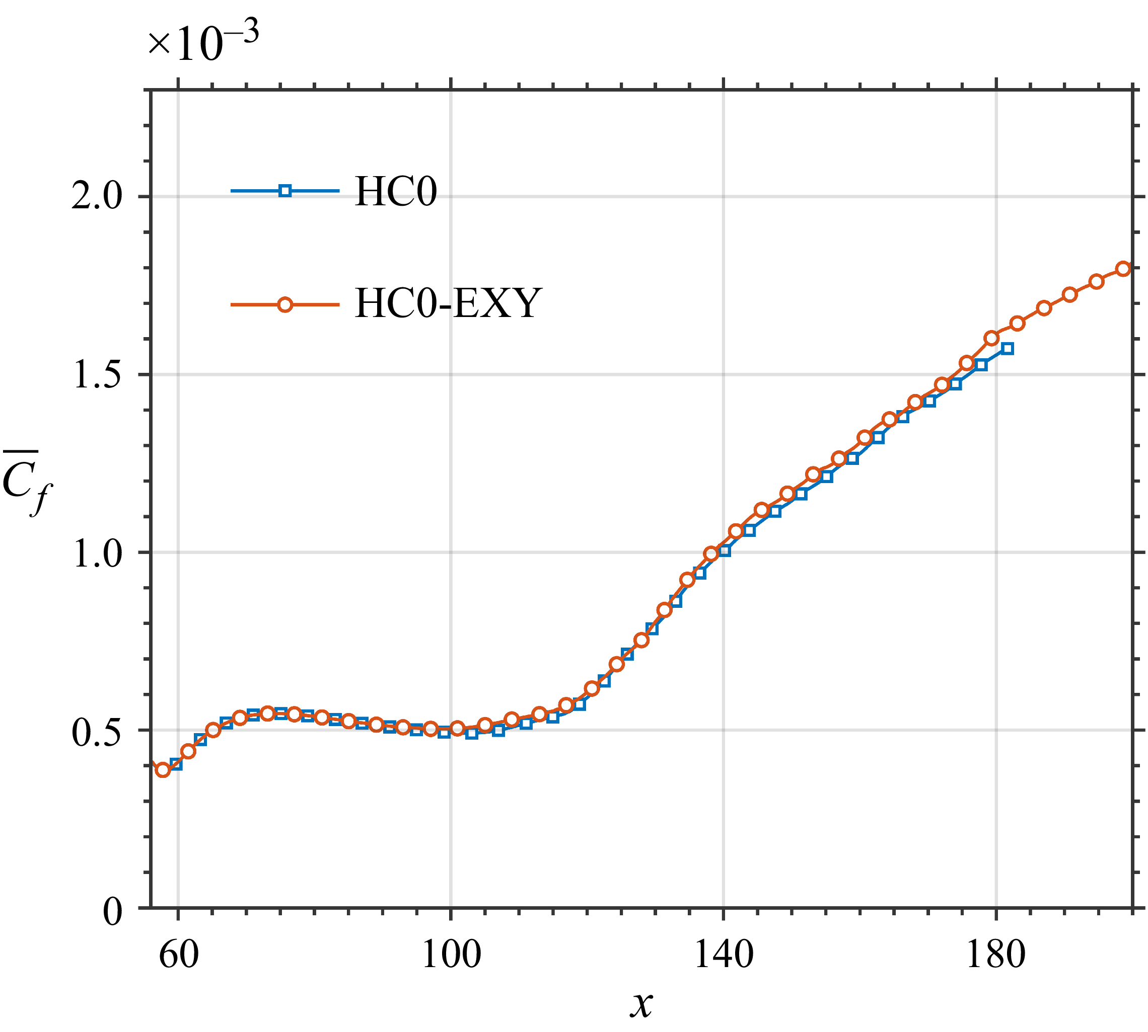
 C¯f
 x
 y

 x=90
 z=0
 z=2.5
 C¯f
 x
 y
 z
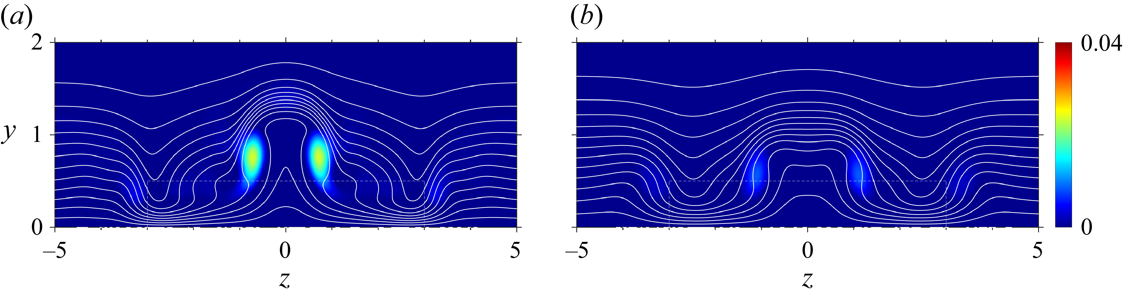
 Q
 x=90
 [0,2.5]
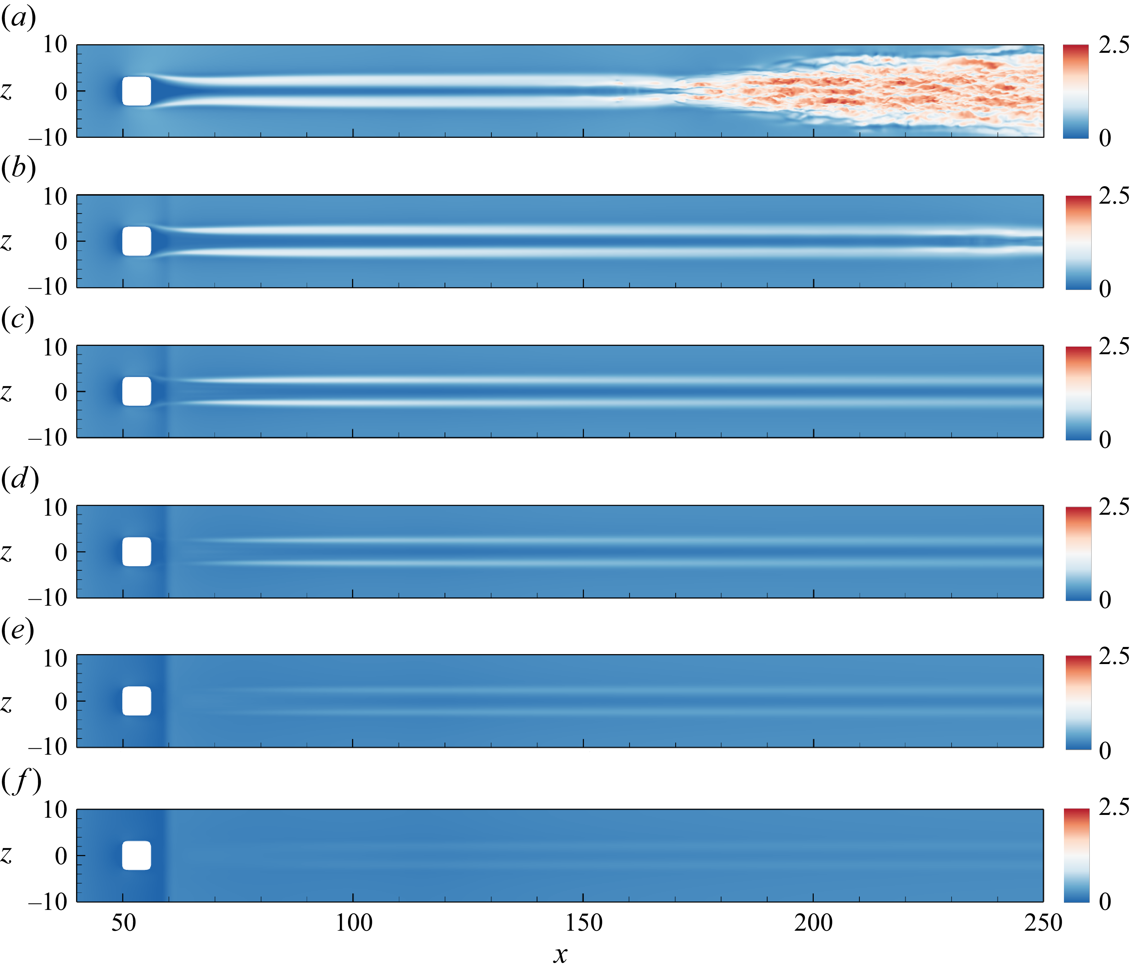
 u
 y=0.2
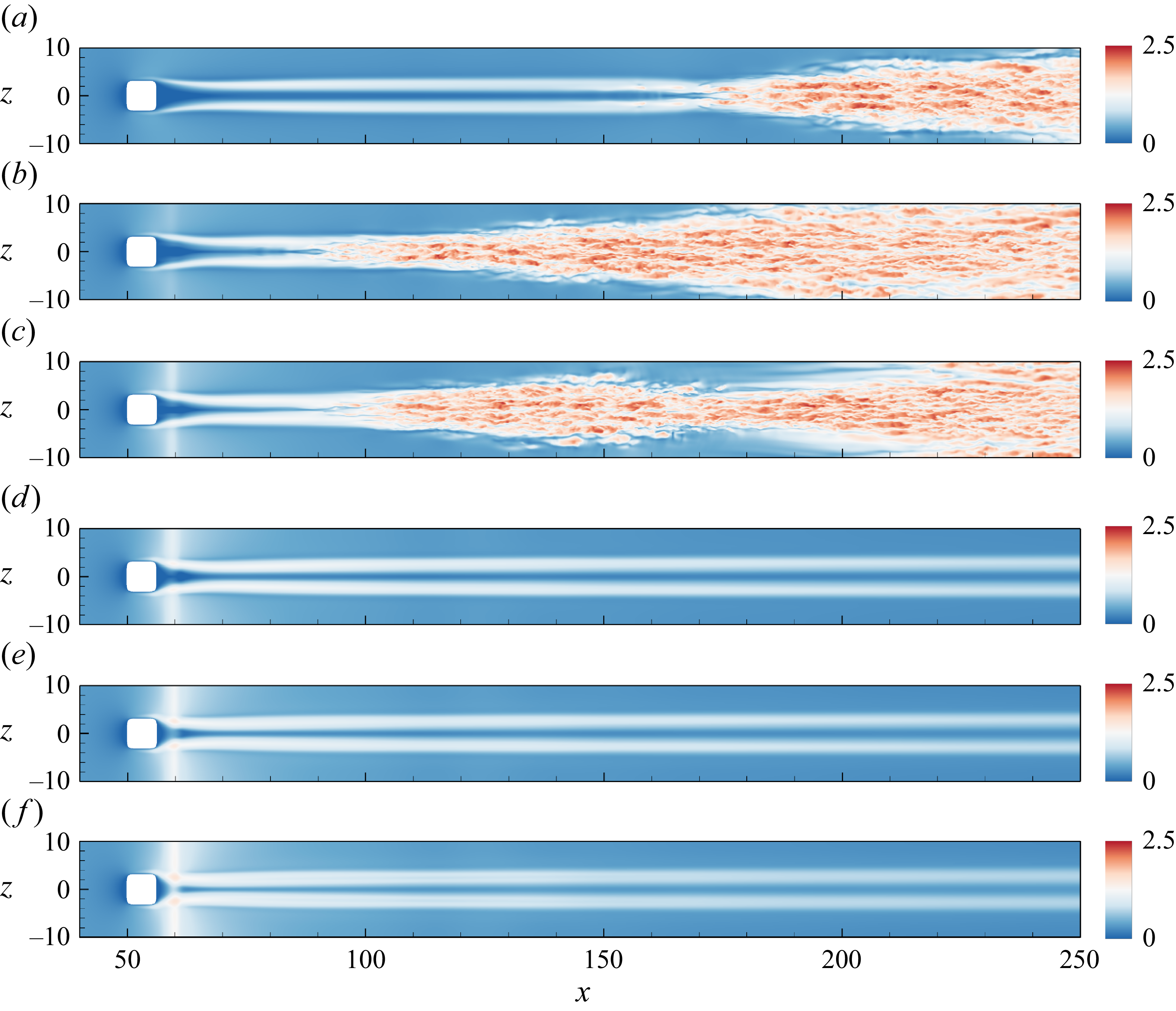
 u
 y=0.2


